

Submitted:
30 September 2026
Posted:
02 October 2026
You are already at the latest version
Abstract
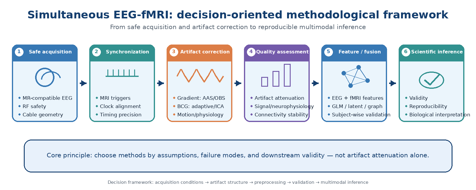
Simultaneous EEG-fMRI combines the temporal resolution of electrophysiology with the spatial coverage of blood-oxygen-level-dependent imaging, but these benefits come with substantial methodological constraints. We examine simultaneous EEG-fMRI as a linked acquisition-to-inference workflow, with the two modalities treated as interdependent during preprocessing and analysis. We consider MRI-compatible acquisition and safety, temporal synchronization, gradient and ballistocardiographic artifact correction, EEG and fMRI preprocessing, quantitative quality assessment, connectivity analysis, and multimodal fusion. We focus on the assumptions and failure modes of each approach, preservation of neural information, and evidence for generalization beyond the setting in which each method was developed. The available literature does not support a single artifact-correction strategy for all recordings. Template methods remain effective when artifact timing and morphology are stable, whereas basis-set, adaptive, reference-based, and learning-based approaches may be more appropriate when contamination varies over time or real-time operation is required. Because preprocessing can alter spectral estimates, connectivity, and network organization, residual artifact amplitude alone is an inadequate measure of success. We propose a decision-oriented framework in which acquisition conditions, artifact structure, analysis target, and validation level are considered together when selecting an EEG-fMRI pipeline.
Keywords:
EEG-fMRI
; ballistocardiographic artifact
; gradient artifact
; neuroimaging preprocessing
; functional connectivity
; multimodal fusion
; reproducibility
1. Introduction
EEG and fMRI observe brain activity through very different biophysical processes. EEG is directly sensitive to rapid electrical field changes at the scalp, whereas fMRI primarily reflects slower blood-oxygen-level-dependent responses with broad spatial coverage. Recording the two modalities at the same time is valuable when the question depends on within-session correspondence, such as trial-to-trial fluctuations or changes in brain state. Simultaneous acquisition is not automatically preferable to separate sessions because it restricts how each modality can be optimized [1,2,3,4,5]. The same MRI environment that makes concurrent measurement possible also introduces unusually large contaminants into the EEG. Gradient switching, ballistocardiographic (BCG) effects, head and cable motion, and other physiological or environmental signals can overlap genuine neural activity. In this setting, preprocessing is better viewed as a signal-reconstruction problem than as ordinary noise removal [6,7,8,9,10,11].
The conceptual basis of simultaneous EEG-fMRI and the main asymmetric integration strategies were established in early methodological work and reviews. Later studies focused more directly on artifact correction, acquisition practice, and reporting quality [1,2,3,9,10]. Recent work has expanded to high-field acquisition, real-time correction, open benchmarking datasets, connectivity-based fusion, self-supervised learning, group joint ICA, and mechanistic whole-brain models [12,13,14,15,16,17,18,19,20,21]. This expansion creates a practical problem: a preprocessing choice that makes the EEG appear cleaner may still change the spectral features, connectivity estimates, or multimodal relationships on which the scientific conclusion depends.
The review therefore follows the full path from acquisition to inference. We do not attempt to identify a universally superior correction algorithm. Instead, we ask how acquisition conditions and artifact structure constrain method choice, where each approach is likely to fail, what neural information may be altered, and how correction quality should be evaluated for the analysis that follows. Safety, synchronization, artifact correction, modality-specific preprocessing, multimodal integration, connectivity, and reproducibility are considered within this common framework. The working criterion throughout is whether a pipeline removes enough non-neural contamination to support a valid analysis without unnecessarily damaging the neural information of interest.
2. Review Approach and Critical Appraisal Framework
This is a critical methodological review rather than a formal systematic review or meta-analysis. Foundational papers were retained because many current EEG-fMRI pipelines still depend on acquisition, synchronization, and artifact-correction principles introduced in earlier work. More recent methodological comparisons, safety studies, open datasets, real-time frameworks, and multimodal-learning studies were used to examine where those assumptions remain useful, where they have been challenged, and which questions are still unresolved. The literature was checked through September 2026 [1,2,3,9,10,12,13,14,15,16,17,18,19,20,21,22].
Five connected domains structure the review: acquisition and safety; artifact generation and correction; signal quality and preservation of neurophysiology; multimodal integration and connectivity; and reproducibility together with emerging computational approaches. They are considered as parts of one pipeline because choices made early in acquisition and preprocessing can change the features, connections, and multimodal relationships estimated later.
The same appraisal questions are used repeatedly across these domains. What does a method assume about the data? Under what acquisition or physiological conditions is that assumption likely to fail? Which neural features might be attenuated or distorted? Has the method been tested independently of the group that developed it? Finally, is the method suitable for the specific downstream analysis? Framing the comparison in this way helps separate long-standing use from actual evidence of robustness.
The review synthesizes major EEG-fMRI methodological lineages rather than cataloguing every publication. The selected literature represents major methodological lineages, influential foundational studies, comparative evaluations, and well-documented recent developments. When peer-reviewed evidence was available, preprints were not used as the main basis for methodological recommendations. The overall acquisition-to-inference architecture used to organize this review is summarized in Figure 1.
3. Why Simultaneous EEG-fMRI Is Methodologically Difficult
EEG and fMRI can be treated as two observation systems that sample partly shared neural and physiological processes in different ways. In simplified form:
EEG(t) = H_E [z(t)] + ε_E(t)
fMRI(t) = H_F [z(t)] + ε_F(t)
Here, z(t) denotes latent neural and physiological states; H_E represents the electrophysiological measurement process; H_F includes neurovascular transformation and BOLD measurement; and the epsilon terms represent modality-specific noise. This is a deliberately simplified representation and is not intended as a complete generative model. EEG and fMRI are not interchangeable measurements of the same quantity. They provide different views of partially shared processes [1,2,3].
The cross-modal relationship is further complicated by neurovascular coupling and by the large difference in temporal response between electrophysiology and BOLD. In a conventional EEG-informed fMRI analysis, an EEG-derived feature F_EEG(t) is commonly converted into a delayed BOLD predictor by convolution with a hemodynamic response function:
R(t) = F_EEG(t) * HRF(t)
How well this approximation works depends on the EEG feature, experimental design, brain region, and assumed hemodynamic response. A direct correlation between EEG and fMRI values sampled at the same clock time is therefore usually an incomplete description of electrophysiological-hemodynamic coupling [2,3,4,10].
The MRI environment introduces a second source of difficulty. The recorded EEG can be represented conceptually as:
X(t) = N(t) + G(t) + B(t) + P(t) + M(t) + ε(t)
In this expression, N(t) is neural EEG, G(t) gradient artifact, B(t) BCG artifact, P(t) other physiological contamination, M(t) motion-related contamination, and epsilon(t) residual noise. Gradient artifact is usually highly structured and sequence locked, whereas BCG and motion are less stationary and vary more across participants and recording conditions. Several of these components overlap genuine EEG in both time and frequency, so they cannot be separated simply by removing an isolated spectral band [6,7,8,9,11].
This overlap makes artifact correction intrinsically ambiguous. The recorded data do not provide a perfect label indicating which variance is neural and which is artifactual. A method can reduce scanner-related contamination while at the same time altering neural waveforms, power estimates, phase relationships, or the covariance structure used for connectivity analysis. Comparative work now shows that such preprocessing choices can affect downstream neurophysiological and network results, not only the visual appearance of the cleaned signal [8,22,23].
Greater artifact attenuation is not necessarily better. Correction should be judged in relation to the acquisition conditions, the neural feature being studied, and the analysis that follows. A pipeline suitable for an ERP analysis may not be optimal for high-frequency power, source reconstruction, connectivity, or multimodal prediction [8,9,22,23].
4. MRI-Compatible EEG Acquisition and Safety
4.1. Hardware Configuration
A present-day simultaneous EEG-fMRI setup usually includes MRI-compatible electrodes and leads, an MRI-compatible amplifier, ECG and, where appropriate, EOG or other physiological channels, plus an interface that links EEG timing to the MRI sequence. The shift from long analog signal paths toward in-bore digitization and optical transmission has reduced several transmission-related problems and made continuous recording more practical [1,3,10].
Hardware choices need to reflect both the acquisition environment and the planned analysis. High EEG sampling rates have often been used because gradient artifacts contain steep transitions and considerable high-frequency energy; Allen et al., for example, used 5 kHz in an early continuous EEG-fMRI implementation. This value is not a universal requirement. Effective correction has also been demonstrated at lower sampling rates, and the appropriate rate depends on amplifier bandwidth, sequence timing, synchronization accuracy, artifact morphology, storage constraints, and the EEG frequency range of interest [6,7].
These acquisition parameters are not independent of preprocessing. Sampling rate, amplifier characteristics, and clock synchronization shape the artifact that is actually digitized and, in turn, affect which correction strategies are likely to work reliably.
4.2. Electrode and Cable Configuration
Electrode placement and cable routing matter for both safety and signal quality. Conductive loops should be avoided, leads should follow validated routing schemes, and unnecessary cable length should be minimized where the hardware permits. More generally, the relevant object is the whole conductive geometry: electrodes, leads, amplifier location, and participant position together determine susceptibility to MRI-induced and environmental interference.
The 4 T study by Assecondi et al. provides a clear example. A more compact arrangement with shorter EEG cables was substantially less sensitive to external noise and MR-induced artifacts. The study does not support prescribing one cable length for every system; it instead identifies cable geometry as an acquisition variable that should be standardized and reported [24].
4.3. RF-Induced Heating and Safety
RF-induced heating remains a major safety concern because conductive electrodes and leads interact with the transmitted RF field and can support induced currents or local temperature increases. The amount of heating depends on the complete configuration, including field strength, RF coil, sequence, electrode properties, cable geometry, participant positioning, and RF exposure [25].
Accordingly, an EEG system being labeled 'MR compatible' does not by itself establish safety for every scanner and sequence. Safety has to be evaluated at the level of the full setup. In practice, this means avoiding loops, using manufacturer-validated arrangements, limiting unnecessary conductive structures, respecting validated RF exposure conditions, and carrying out configuration-specific testing when required.
Recent 7 T studies show that simultaneous EEG-fMRI can be implemented safely and with high spatial resolution when the system is engineered and tested for that purpose. Those results are encouraging, but they should not be extrapolated to different amplifiers, caps, coils, sequences, or routing arrangements without additional validation [16,25].
4.4. Temporal Synchronization
Synchronization becomes especially important when artifact removal depends on the repeatability of the gradient waveform. Small timing errors can change the samples used to represent a rapidly varying artifact and thereby reduce the effectiveness of template subtraction.
Mandelkow et al. showed that locking the EEG sampling clock to the MRI sequence improves template-based gradient-artifact correction and increases usable EEG bandwidth. Precise hardware synchronization is therefore particularly valuable when AAS or related template methods are used [26].
Not every preprocessing method depends equally on clock locking, so synchronization should not be described as an absolute prerequisite for all pipelines. The timing architecture should be appropriate for the correction method, and the achieved precision should be documented.
4.5. Acquisition Design
Experimental design must accommodate the requirements of both modalities. Continuous acquisition is commonly used because it preserves trial-level and state-dependent correspondence between EEG and BOLD. Interleaved designs can still be useful when reducing MRI-induced contamination is more important than maintaining uninterrupted temporal overlap [5,10].
Stimulus timing, trial spacing, behavioral responses, sequence parameters, and the expected hemodynamic response should therefore be planned together. Optimizing one modality in isolation can compromise the other. In practice, hardware configuration, safety, synchronization, and experimental timing jointly determine both the quality of the raw data and the artifact structure that must later be modeled. These acquisition, safety, synchronization, and experimental-timing considerations are summarized in Figure 2.
5. Artifact Sources and Structure
Gradient artifact, BCG, motion, physiological signals, and scanner or equipment noise differ in amplitude, temporal structure, predictability, and origin. Their magnitude is only part of the problem; equally important is whether their structure is stable enough to be modeled across time [7,8,9,11]. The principal sources of contamination and their differing temporal structures are summarized in Figure 3.
Gradient artifact is usually the most structured component. It is generated primarily by rapidly switching magnetic-field gradients and is strongly time-locked to the MRI sequence. Its large amplitude and high repeatability make template-based approaches feasible, although even small timing errors, motion, or changes in acquisition conditions can reduce this repeatability. In contrast, BCG artifact is cardiac-related but substantially less stationary: its morphology varies across heartbeats, channels, head positions, field strength, and participants. This difference explains why methods that perform well for gradient artifact may be less effective for BCG contamination [6,7,8,9,27].
Motion is particularly troublesome because it is not only non-stationary but also interactive. Movement of the head, electrodes, or leads can generate artifact directly and can also change the morphology of both gradient and BCG contamination. A fixed template that performs well during a stable period may therefore fail after a change in head or cable position [9,10,11].
Ocular activity, muscle activity, respiration, and other physiological signals can occupy the same frequency range as neural EEG. Environmental and scanner-related interference adds further narrowband or broadband components, often in a site- or hardware-dependent manner. This overlap is why aggressive filtering or component rejection can improve apparent cleanliness while removing physiologically meaningful signal.
Correction methods are therefore best matched to the structure of the contamination. Strongly periodic artifacts can often be handled with template or basis-set approaches, whereas non-stationary contamination may require adaptive, reference-based, component-based, or learned models. Gradient artifact and BCG are considered separately below because their predictability and failure modes are quite different.
6. Gradient Artifact Correction
Gradient artifact is usually the largest and most regular contaminant in simultaneous EEG-fMRI. Because it is tightly linked to MRI gradient switching, it is more predictable than BCG or motion artifact. At the same time, its amplitude is so large that modest timing error, motion, or sequence-related change can leave substantial residuals. The practical problem is to exploit the artifact's regularity without subtracting EEG activity that happens to share the same temporal or spectral structure [6,7,8,9].
Available correction methods make different compromises. Template, basis-set, moving-average, adaptive, and data-driven approaches differ in how much stationarity they assume, how strongly they depend on synchronization, and how easily they can absorb neural variance into the artifact model. Those differences are more informative for method choice than how frequently a method has been used historically. The main trade-offs among gradient-artifact correction strategies are summarized in Figure 4.
6.1. Average Artifact Subtraction (AAS)
AAS, introduced by Allen et al., is the classical template-subtraction approach. Repeated slice- or volume-related epochs are averaged to estimate the gradient waveform, and the resulting template is subtracted from each occurrence [6].
AAS is simple, interpretable, computationally inexpensive, and widely established, but its reliance on reproducible artifact morphology is also its main limitation. The method assumes that the artifact remains sufficiently reproducible for an average waveform to represent individual epochs. Timing jitter, head or cable movement, and sequence-related changes violate that assumption and leave structured residuals. AAS is consequently best suited to recordings with stable artifact morphology and precise synchronization [6,9,26].
6.2. Sliding-Window and Local Template Approaches
Local-template approaches use neighboring artifact epochs rather than a single template estimated over the entire recording. This allows gradual changes in morphology to be followed, but the window length becomes an important tuning parameter. A long window is stable but slow to adapt; a short window follows change more closely but is more likely to incorporate neural activity into the artifact estimate. The selected window should therefore be reported explicitly [9].
6.3. Optimal Basis Sets (OBS)
OBS replaces a single artifact waveform with a low-dimensional set of basis functions, usually derived with principal-component methods. The basis can represent structured changes in artifact morphology that a fixed average cannot capture [7].
This added flexibility introduces a trade-off. Too few components can leave systematic residuals; too many can begin to describe neural variance as artifact. The number and interpretation of basis components are therefore part of the method, not merely implementation details. Evaluation should include preservation of the target EEG feature as well as attenuation of the artifact [7,8,22].
6.4. Optimized Moving-Average (OMA)
Optimized moving-average methods exploit the periodicity of gradient artifact without relying only on epoch-wise template subtraction. Ferreira et al. reported effective attenuation and suggested advantages when template timing is imperfect and when higher-frequency EEG is of interest [28].
OMA may be most useful when periodicity remains strong but exact template alignment is difficult. Its performance still depends on the selected averaging parameters and on the artifact remaining sufficiently regular over time. Given the smaller comparative literature, it is more reasonable to view OMA as an alternative for selected conditions than as a general replacement for AAS [9,28].
6.5. Adaptive, Reference-Based, and Data-Driven Approaches
Adaptive and reference-based approaches attempt to follow changes in contamination rather than assuming a fixed artifact. They use measured reference signals, regression, adaptive filters, or related models to update the artifact estimate over time. This can be advantageous during non-stationarity, but performance depends heavily on reference quality and on keeping the reference sufficiently insensitive to the neural signal of interest [9].
Learning-based methods extend this idea by estimating nonlinear mappings between contaminated and corrected EEG. They may be useful for complex or time-varying artifact, particularly in online applications, but they introduce a different set of concerns: dependence on the training distribution, generalization across subjects and scanners, and limited interpretability. EEG-LLAMAS and NeuXus are examples of causal, low-latency processing. Their value, however, should be judged by end-to-end latency and preservation of task-relevant EEG rather than by offline attenuation alone [12,17].
6.6. Critical Comparison and Method Selection
AAS remains the most familiar reference method, but the literature does not establish it as universally superior. Independent comparisons of newer methods are still relatively sparse, and some approaches have mainly been evaluated by the groups that introduced them. This makes acquisition-specific benchmarking more informative than historical prevalence [9,22].
- Highly stable, well-synchronized artifact: AAS or related template-based correction.
- Slowly varying artifact: local or sliding templates.
- Structured morphology variation: OBS.
- Periodic artifact with timing mismatch or high-frequency preservation requirements: OMA.
- Strongly non-stationary or motion-sensitive artifact: adaptive or reference-based approaches.
- Complex nonlinear or real-time settings: data-driven or machine-learning approaches, provided that generalization is independently validated.
Lower residual artifact amplitude alone is insufficient evidence of better preprocessing. The preferred correction is the one that reduces contamination enough for the intended analysis while retaining the neural information on which that analysis depends.
7. BCG Artifact Correction and EEG Preprocessing
BCG is usually less predictable than gradient artifact. It is linked to the cardiac cycle, but its waveform is shaped by several processes, including cardiac contraction, blood movement, head rotation, electrode motion, static field strength, channel geometry, and participant position. Both amplitude and spatial variability tend to increase with field strength, and the artifact can occupy frequency bands that are physiologically relevant [9,11,27].
7.1. Template- and Basis-Set Methods
Cardiac-triggered AAS and OBS are widely used because the ECG R-peak provides a convenient timing reference. Beat-to-beat BCG morphology, however, is not fixed, and R-peak timing captures only part of the mechanical and electromagnetic processes that generate the artifact. OBS can accommodate structured variation better than a single template, although the number of basis components again determines the balance between artifact modeling and neural-signal preservation [7,11,29].
7.2. Component-Based Methods
ICA and related blind-source methods are useful when a substantial fraction of BCG variance is concentrated in identifiable components. The difficulty is that statistical independence does not guarantee physiological purity; a component can contain both cardiac artifact and neural activity. Decisions to reject components are therefore more defensible when they combine ECG association, temporal morphology, spectra, scalp topography, and reproducibility rather than relying on a single threshold. Reviews generally support ICA as a complementary step rather than as a universally reliable stand-alone BCG solution [9,11].
7.3. Reference-Based and Adaptive Methods
Reference-layer sensors, carbon-wire loops, motion sensors, and adaptive regression try to measure artifact-related variance directly instead of inferring it only from scalp EEG. Direct measurement can be useful for non-stationary pulse and motion effects. It also creates a clear requirement: the reference must be strongly sensitive to contamination while remaining weakly sensitive to neural activity. The mapping between reference and scalp artifact can change with posture, field strength, and hardware configuration, so reference quality needs to be checked rather than assumed [9,12,18].
7.4. Deep Learning and Real-Time BCG Correction
McIntosh et al. used recurrent neural networks to model the relationship between ECG and BCG-contaminated EEG and reported reduced BCG power while retaining task-relevant classification. Lin et al. later proposed a GAN-based approach that did not require an additional reference signal and reported stronger suppression than the comparison methods used in that study. These results establish feasibility, but they do not yet remove the need for independent testing across scanners, montages, tasks, and participant groups [30,31].
Real-time correction adds constraints that are less important offline. The algorithm must be causal, fast, and stable enough to operate continuously. EEG-LLAMAS combines reference-layer measurements with causal Kalman filtering and reported sub-50-ms average lag; NeuXus provides open-source pulse-artifact correction with execution times compatible with neurofeedback. In this setting, total system delay and recovery of the neural feature used for feedback are more informative than the appearance of an offline-cleaned trace [12,17].
7.5. From Artifact Correction to a Complete EEG Preprocessing Pipeline
EEG preprocessing is a sequence of dependent decisions. It extends beyond a single artifact-removal operation. Raw-data checks and timing verification come first, followed by gradient correction, BCG and residual physiological correction, and then the channel, reference, filtering, epoch, and feature operations required by the study. This order matters because interpolation, re-referencing, filtering, and ICA change the data distribution seen by later steps and can alter both artifact estimates and neural covariance [9,10,32].
7.6. Raw-Data and Timing Quality Control
Before aggressive cleaning, basic acquisition integrity should be established. Channel labels and montage, sampling rate, reference and ground, amplifier saturation, trigger integrity, ECG/EOG quality, missing samples, flat or noisy channels, and correspondence between MRI triggers and image volumes all need to be checked. For template-based gradient correction, it is also important to look for missing or duplicated slice/volume events and changes in the number of samples per artifact epoch. Acquisition failures are easier to interpret when they are identified explicitly rather than hidden by later interpolation or resampling [7,9,10].
7.7. Residual-Artifact Inspection
Residual artifact should be examined in more than one representation. Peaks at the slice or volume repetition frequency and its harmonics can indicate incomplete gradient correction, while recurrent waveforms aligned to ECG R-peaks suggest remaining BCG. Time traces, spectra, topography, ECG association, and, where available, outside-scanner or scan-off recordings provide complementary information. A lower global RMS can therefore coexist with greater distortion in a particular frequency band or network measure [22,23].
7.8. Filtering, Bad Channels, Interpolation, and Re-Referencing
Filter settings should follow the inferential target. A high-pass cutoff that is useful for drift suppression may attenuate slow cortical activity or alter ERP baselines; a low-pass cutoff chosen mainly to hide residual scanner noise may remove gamma or other high-frequency information. Filter type, order, cutoffs, phase characteristics, and whether filtering occurred before or after artifact correction should be reported [32].
Bad-channel detection is best performed before average re-referencing, otherwise one persistently noisy channel can contaminate the reference itself. Interpolation should be conservative because it changes spatial covariance. Re-referencing likewise affects source and connectivity estimates, so the acquisition reference and the rationale for any offline reference need to be stated explicitly [32].
7.9. Epoching, Baseline Correction, and Rejection
Epoching usually follows removal of the dominant scanner artifacts unless the chosen correction method requires event-locked epochs. Baseline correction deserves particular care when slow scanner drift or physiological contamination makes the pre-stimulus period non-neutral. Rejection rules should distinguish acquisition failure from physiological artifact, be defined before group inference, and be reported at participant and trial level. Both excessive exclusion and retention of severely contaminated trials can bias the final result.
7.10. Feature and Source-Level Preparation
After cleaning, EEG can be expressed as time-domain responses, spectra, time-frequency features, source estimates, or connectivity. Each representation inherits uncertainty from earlier preprocessing. Source analysis additionally depends on electrode localization, head modeling, reference choice, and inverse-model assumptions. Connectivity is especially sensitive to operations that alter phase or covariance, including filtering, interpolation, referencing, and ICA. Measures such as imaginary coherency or weighted phase-lag indices can reduce sensitivity to instantaneous volume-conduction effects, but only under the assumptions of those measures [33,34].
7.11. Recommended EEG Preprocessing Decision Rule
A reasonable default is to verify timing and raw integrity first, then correct gradient artifact, address BCG and other physiological contamination, apply conservative channel/reference/filter operations, and perform epoch-level QC before deriving ERP, power, source, or connectivity measures. This sequence is not mandatory for every pipeline; adaptive and real-time methods may require a different order. Any departure from the default should be motivated by the algorithm being used and checked against the downstream analysis. The proposed EEG preprocessing sequence, quality-control targets, and downstream risks are summarized in Table 1.
8. Quantitative Quality Assessment
Artifact correction has traditionally been judged by two questions: how much contamination was removed, and how much biological EEG was preserved. Connectivity, prediction, and multimodal learning add another requirement: whether the downstream result remains valid. A method that produces a smaller residual artifact but erases a known EEG response or changes network organization has not succeeded for that analysis [8,22,23].
We therefore use a five-level validation scheme. The first level measures artifact attenuation. The second asks whether waveform or signal fidelity is retained. The third tests expected spectral and temporal neurophysiology. The fourth examines the stability of connectivity and graph organization. The fifth asks whether the scientific conclusion itself is robust to preprocessing. Higher levels do not replace basic signal QC; they extend it to the quantities that the study ultimately interprets. This five-level validation framework is summarized in Figure 5.
The study by Kraljic et al. illustrates this broader approach by comparing accessible correction methods against outside-scanner EEG with both spectral and time-domain outcomes. More recent work has taken the same idea to connectivity and graph measures, where BCG correction can produce method-dependent changes in network topology. These results support validation against the target signal or inference rather than a single universal ranking of correction algorithms [22,23].
9. fMRI Preprocessing in the Multimodal Pipeline
fMRI preprocessing is part of the same multimodal measurement chain and should be matched to the EEG analysis rather than treated as a fixed recipe. Volume handling, motion correction, physiological denoising, temporal filtering, normalization, smoothing, and parcellation all shape the BOLD features that will later be related to EEG. Frameworks such as fMRIPrep make core preprocessing more transparent and reproducible, but nuisance modeling and connectivity preparation still depend on the analysis [35,36].
9.1. Non-Steady-State Volumes and Acquisition Integrity
Initial volumes can show non-steady-state magnetization and may need to be removed or modeled. The number should be determined from the sequence rather than from a fixed convention. In simultaneous studies, any discarded fMRI volumes must also be reconciled with EEG timing so that event markers and EEG-derived regressors remain aligned with the BOLD series that is actually analyzed.
9.2. Motion Correction as a Cross-Modal Confound
Head motion affects BOLD through displacement, spin-history effects, susceptibility changes, and altered alignment between anatomy and the acquisition grid. In simultaneous EEG-fMRI there is an additional consequence: a change in head position also changes electrode and cable geometry, which can modify both gradient and BCG artifact. Motion is therefore a cross-modal confound. Framewise displacement, DVARS or comparable metrics, censoring decisions, and participant-level exclusion rules should be reported when relevant [9,37].
9.3. Slice Timing, Distortion, Registration, and Normalization
Slice-timing correction is not automatically required for every dataset; its value depends on TR, multiband factor, and the temporal model used in the analysis. Susceptibility and geometric-distortion correction become especially important when precise ROI correspondence is required. Registration should establish consistent relationships among functional images, anatomical images, and the parcellation used for multimodal analysis, and normalization should be inspected rather than assumed to have succeeded [35].
9.4. Physiological Noise Correction
Cardiac and respiratory processes contribute structured variance to BOLD. With physiological recordings, RETROICOR-type regressors can model periodic effects explicitly. aCompCor takes a data-driven route using components from white-matter and CSF compartments, while ICA-based methods such as ICA-AROMA identify motion-related components from spatial and temporal features. Because these approaches remove different sources of variance, the denoising strategy should be selected for the specific task or connectivity analysis [38,39,40,41].
9.5. Nuisance Regression and Temporal Filtering
Nuisance models may include motion terms and derivatives, physiological regressors, white-matter/CSF components, global signal terms, or identified noise components. Filtering and regression are mathematically coupled, and their order affects temporal structure and degrees of freedom. This is particularly important for functional connectivity, where different confound strategies can produce materially different motion relationships and network estimates. Global signal regression remains analysis dependent and should be stated and justified explicitly [36,37].
9.6. Spatial Smoothing
Smoothing is another analysis-dependent choice. Conventional activation studies may benefit from spatial smoothing, whereas fine-grained ROI connectivity, laminar or high-resolution analyses, and cross-modal node matching may require little or none. Excessive smoothing can blur network boundaries and inflate apparent coupling between nearby regions. Any gain in signal-to-noise ratio therefore has to be balanced against the loss of spatial specificity [42].
9.7. ROI Extraction and Cross-Modal Node Correspondence
At ROI or graph level, the parcellation itself becomes part of the method. The atlas should be compatible with the spatial precision of the fMRI data and with what can realistically be localized from EEG source estimates. Node labels, hemisphere assignments, and ordering must match across modalities, and the mapping from EEG sources to fMRI ROIs should be explicit. This is essential for connectome comparisons and multilayer graphs [14].
9.8. fMRI Functional-Connectivity Preparation
For ROI-to-ROI connectivity, BOLD time series are extracted after the selected denoising strategy. Pearson correlation is common, but partial correlation, precision-based measures, ICA-derived connectivity, and dynamic approaches answer somewhat different questions. Because edge weights are sensitive to motion and nuisance regression, connectivity studies should report motion QC and, when feasible, test whether key findings survive plausible preprocessing alternatives [36,37].
9.9. Multiband-Specific Artifacts
Multiband acquisition brings sequence-specific artifacts of its own. Tubiolo et al. described a shared non-neural signal across simultaneously acquired slices and proposed Multiband Artifact Regression in Simultaneous Slices (MARSS). The MARSS example shows that acceleration can introduce structured residuals that are not necessarily addressed by a conventional preprocessing pipeline [43].
9.10. Critical Recommendation for Simultaneous EEG-fMRI
For simultaneous EEG-fMRI, fMRI preprocessing is best evaluated by its effect on the multimodal quantity being interpreted. Task activation, resting-state connectivity, dynamic connectivity, high-resolution ROI analysis, and EEG-informed GLMs need not favor the same nuisance strategy. A final QC check should also confirm that EEG-derived features remain correctly aligned with the retained fMRI time series after volume removal, censoring, and other temporal transformations. The principal fMRI preprocessing operations and their cross-modal implications are summarized in Table 2.
10. Multimodal Integration and Data Fusion
10.1. EEG-Informed fMRI
EEG-informed fMRI is the classical asymmetric approach. An EEG feature is extracted, aligned in time, usually convolved with an HRF, and entered into a voxelwise or ROI-level GLM. The method is readily interpretable: rapid electrophysiological variation can be related to spatially resolved BOLD responses. It has been used for oscillatory power, event-related activity, vigilance, sleep, and epileptiform discharges [3,4,10].
10.2. fMRI-Informed EEG
In the reverse direction, fMRI can provide a spatial prior or constraint for EEG source reconstruction and interpretation. This can reduce ambiguity in the EEG inverse problem, but spatial overlap should not be equated with identical generators. fMRI reflects hemodynamic consequences of neural activity, whereas EEG reflects electrical field potentials, so the strength of an fMRI prior should be proportional to the claim being made.
10.3. Symmetric and Joint Modeling
Symmetric approaches avoid assigning one modality the role of predictor and the other the role of outcome. Instead, both contribute to a shared or coupled latent representation. This distinction remains informative even though many practical pipelines contain elements of both [3,5]. The major EEG-fMRI integration and data-fusion strategies are summarized in Figure 6.
10.4. Multivariate Statistical Learning
Multivariate methods such as ridge regression, relevance vector machines, canonical correlation analysis (CCA), partial least squares (PLS), and joint ICA can capture distributed relationships that are difficult to see in a series of univariate voxelwise tests. De Martino et al. demonstrated this potential in simultaneous EEG-fMRI. The result, however, should be interpreted within the validation design of that study rather than as evidence that one multivariate model is generally superior across datasets [4].
10.5. Feature-Level, Latent, and Decision-Level Fusion
Early fusion simply concatenates features from the two modalities before fitting a model. Its transparency is an advantage, but the feature spaces can be badly unbalanced: EEG spectral or connectivity features and fMRI features may differ greatly in scale and dimensionality. Standardization, feature selection, and dimensionality reduction must therefore be learned within the training data rather than applied once to the full dataset.
Intermediate fusion first learns a representation within each modality and then combines those representations. Deep encoders, variational autoencoders, contrastive objectives, and cross-modal attention all fit this general pattern. The 2025 MCSP framework, for example, was designed to align temporal, spectral, and spatial information across EEG and fMRI rather than relying on direct feature concatenation [15].
Late fusion keeps modality-specific models separate and combines their predictions only at the decision stage. This modularity is useful when the modalities require very different preprocessing or model classes, although interactions that occur before the final prediction may be missed. The choice among early, intermediate, and late fusion is consequently a design decision tied to the hypothesis and sample size, not a hierarchy of sophistication.
10.6. Regression and Covariance-Based Prediction
Cross-modal prediction asks whether features from one modality predict spatial patterns or outcomes in the other. Ridge regression is useful when predictors are numerous and correlated; sparse Bayesian models can reduce the effective feature set; and PLS emphasizes shared covariance. Whatever the model, validation should be done on held-out participants. Random trial-level splits can otherwise allow participant-specific structure to appear in both training and test sets [4].
10.7. CCA, PLS, and Joint ICA
CCA identifies linear combinations of EEG and fMRI variables with maximal correlation, whereas PLS focuses on covariance with a target representation. Joint ICA estimates components shared across suitably scaled modality-specific observations. These methods are generally easier to interpret and fit than many deep architectures, but their results can still depend strongly on scaling, dimensionality reduction, and the assumed mixing structure.
Group joint ICA (gjICA), introduced in 2026 for concurrent EEG-fMRI, extends this family by aiming to preserve temporal information while estimating multimodal group structure. Its design follows the structure of paired simultaneous data rather than generic concatenation. As with any new fusion approach, broader independent replication and comparison with simpler latent-variable baselines will be important [19].
10.8. Tensor and Matrix-Factorization Fusion
EEG-fMRI data have a natural multiway structure spanning participant, region, frequency, time, trial, and modality. Matrix and tensor factorizations can retain more of that structure than flattening everything into a single vector. Rank selection and model constraints can, however, lead to overfitting or components with limited biological meaning.
10.9. Connectivity-Level Fusion
Connectivity-level fusion treats EEG and fMRI as networks rather than feature vectors. EEG connectivity can be estimated separately by frequency band, while fMRI provides a region-to-region network. The resulting networks can be compared edge by edge, aligned through similarity measures, or treated as layers of a larger graph. This representation is well suited to network hypotheses, but it requires careful handling of EEG volume conduction, fMRI motion and nuisance effects, and node correspondence across modalities [14,33,34].
10.10. Graph-Level Fusion and GNNs
Graph fusion represents ROIs as nodes and within- or between-modality relationships as edges. Multilayer graphs can retain separate EEG frequency networks alongside an fMRI layer, and GNNs can learn representations that use this topology. The added flexibility also creates more analyst choices: edge definition, thresholding, weighting, normalization, oversmoothing, interpretability, and subject-level generalization all become potential sources of instability. Strong regularized and non-graph baselines remain essential comparators.
10.11. Dynamic and Time-Varying Fusion
Dynamic fusion allows the EEG-fMRI relationship to change within a scan. Examples include relating EEG microstates or band-power states to sliding-window or state-based fMRI connectivity. Because BOLD is delayed and sampled much more slowly than EEG, the modalities should not simply be matched sample by sample. Temporal aggregation, state-space models, or explicit hemodynamic modeling are more defensible ways to handle this mismatch [44].
10.12. Real-Time and Closed-Loop Fusion
Real-time fusion adds a hard timing constraint. Artifact correction, feature extraction, alignment, prediction, and feedback all have to fit within the latency tolerated by the neurofeedback paradigm. Offline procedures that depend on noncausal filters, bidirectional smoothing, or long future-looking templates may therefore be unsuitable. Feasibility has been demonstrated in real-time EEG-fMRI systems, but evaluation should report end-to-end delay and whether the targeted neural feature is preserved [12,17].
10.13. How to Choose a Fusion Strategy
The appropriate fusion level depends on the question being asked. An EEG-informed GLM remains a strong choice when a defined electrophysiological event is expected to predict a localized BOLD response. CCA, PLS, or related latent-variable methods are more natural for distributed cross-modal covariance. When participant numbers are limited, regularized regression is usually easier to validate than a deep network. Connectivity or graph fusion is justified when network organization is itself the hypothesis. Deep representation learning becomes more convincing as paired datasets become large and heterogeneous enough for genuinely subject-independent validation. The principal fusion strategies, their trade-offs, and the recommended validation approaches are summarized in Table 3.
11. Connectivity-Based and Network-Level Integration
Recent EEG-fMRI work increasingly emphasizes connectivity and network-level descriptions over regional amplitude measures. EEG can provide frequency-specific connectivity matrices, while fMRI provides region-to-region BOLD connectivity. This creates an appealing multimodal graph representation in which network reconfiguration can be studied across electrophysiological and hemodynamic time scales rather than reducing each modality to a small set of regional summaries.
EEG connectivity can be described with correlation, coherence, phase-locking value, imaginary coherency, weighted phase-lag index, amplitude-envelope coupling, or model-based estimates. fMRI commonly uses Pearson or partial correlation, precision matrices, ICA-derived coupling, and dynamic or state-based measures. These quantities do not have identical statistical or physiological meanings. Similar numbers in an EEG and fMRI matrix should therefore not be interpreted automatically as evidence for the same underlying interaction [33,34].
Meaningful network comparison also requires spatial compatibility. ROI definitions and ordering must match, and modality-specific biases have to be considered explicitly. EEG source leakage can create apparent zero-lag edges, while fMRI connectivity is highly sensitive to motion, physiological noise, global-signal treatment, and temporal filtering. The credibility of a multimodal network result is thus limited by the preprocessing and node correspondence on which it rests [14,37].
11.1. Multilayer Formulation
A multilayer formulation can retain delta, theta, alpha, beta, and gamma EEG networks as separate layers, with another layer representing fMRI connectivity. Cross-layer links can encode region-matched coupling, statistical similarity, or relationships estimated by a model. Keeping the layers distinct avoids collapsing EEG spectral diversity too early and allows explicit hypotheses about reconfiguration across frequency and modality.
11.2. Evidence and Interpretation
Wirsich et al. showed that the relationship between simultaneously recorded EEG and fMRI connectomes can itself carry clinically relevant information in temporal lobe epilepsy. Phadikar et al. combined fMRI spatial-network dynamics with EEG spectral power in resting-state data, providing an example of dynamic multimodal state analysis. Because the latter article was corrected in 2026, version control is particularly relevant when citing rapidly evolving computational work [14,44].
Network correspondence should nevertheless be interpreted cautiously. Similar topology does not imply identical neural generators. Cross-modal similarity can reflect a shared latent state, vascular or behavioral covariation, smoothing, or other preprocessing choices. For network-level claims, sensitivity analysis across parcellations, connectivity metrics, and nuisance strategies is therefore part of the analysis rather than an optional robustness check.
12. Machine Learning, Deep Learning, and Mechanistic Modeling
Machine learning can enter an EEG-fMRI pipeline at several points, from artifact correction and cross-modal prediction to classification, representation learning, graph analysis, and mechanistic modeling. The choice of model should follow the structure of the problem, not the novelty of the architecture. EEG-fMRI datasets often combine high-dimensional features with modest participant counts and repeated observations, a setting in which subject leakage and overfitting can easily dominate apparent performance.
12.1. Graph Neural Networks: Promise and Restraint
GNNs are attractive because brain connectivity already has a graph structure and message passing can use anatomical or functional topology as an inductive bias. The difficulty is that many EEG-fMRI datasets are small relative to the number of nodes and possible edges. Graph thresholding, edge definition, parcellation, normalization, and subject-specific anatomy may influence the representation as much as the learning algorithm itself. GNNs should therefore be compared with ridge or logistic models, linear latent methods, and non-graph neural baselines under participant-wise nested validation.
12.2. Self-Supervised and Cross-Modal Representation Learning
Self-supervised approaches can use paired but weakly labeled data by learning representations that align time, frequency, space, or modality. The 2025 MCSP framework combined domain-specific and cross-modal contrastive objectives for EEG and fMRI. The main validation question is not simply whether a common latent space can be learned, but whether the learned similarity reflects neural correspondence rather than participant identity, site, or preprocessing signatures [15].
12.3. Mechanistic Whole-Brain Modeling
Emerging work also includes mechanistic rather than purely data-driven models. A 2026 whole-brain model used coupled oscillatory dynamics to reproduce features of simultaneous EEG-fMRI across very different time scales, including connectivity and dynamic organization. Such models can make assumptions explicit and support in-silico perturbation, but biological interpretability still depends on identifiability, sensible parameter constraints, and out-of-sample validation [20].
13. Reproducibility, Reporting Standards, and Open Data
Reproducibility requires more than software versioning. Acquisition metadata and artifact-correction details are often incompletely reported, even though those choices can materially affect the signal. Bullock et al. documented gaps in reporting of artifact reduction, while broader EEG/MEG recommendations emphasize transparent acquisition, preprocessing, exclusion, and analysis decisions. BIDS provides a practical structure for preserving multimodal metadata, including the timing information needed to maintain correspondence between EEG and fMRI [9,32,45]. The minimum reporting information needed for reproducible simultaneous EEG-fMRI is summarized in Table 4.
Open datasets allow correction methods to be tested under acquisition conditions that are not under the developer's control. The Gallego-Rudolf dataset, for example, includes EEG outside the scanner, EEG inside the scanner without image acquisition, simultaneous EEG-fMRI, and MRI with and without the EEG cap. This design supports direct comparison of environmental and hardware effects [13].
The 7 T dataset released with the 2025 high-field acquisition framework provides simultaneous recordings at 1.6-mm and 0.8-mm fMRI resolution. Pairing a methodological framework with reusable data makes it possible for other groups to test both acquisition and analysis claims rather than relying only on the original report [16,46].
Two datasets published in 2026 extend these possibilities. Tsutsumi et al. released recordings from 39 healthy adults acquired both inside and outside MR scanners, including carbon-wire-loop channels and a subset of participants scanned at two sites. Cha et al. released simultaneous EEG-fMRI-DTI data across sustained attention, imagery, visual, and resting-state conditions together with preprocessing code. Designs of this kind make cross-pipeline and cross-scanner validation substantially more realistic than it was when many legacy correction methods were introduced [18,21]. Software and toolboxes relevant to EEG-fMRI preprocessing are summarized in Supplementary Table S1.
14. Common Failure Modes and Best-Practice Recommendations
Several problems recur across otherwise different pipelines. Simultaneous acquisition is sometimes treated as inherently preferable even when the hypothesis does not require within-session correspondence. 'MR compatible' can also be interpreted too broadly, despite safety being configuration specific. Template-based gradient correction is vulnerable to timing or morphology changes, while blind ICA rejection can remove neural variance together with BCG. Finally, a fall in global RMS says little about whether spectral, temporal, source, or network information has been preserved [5,8,22,25].
Downstream analysis introduces its own safeguards. Connectivity requires explicit attention to EEG source leakage and to fMRI motion and nuisance effects. Machine-learning studies should separate participants across training and test data and compare complex models with strong regularized baselines. Graph construction and parcellation rules should be specified in advance and tested for sensitivity. Across all of these analyses, acquisition metadata, correction parameters, software versions, and the history of preprocessing decisions need to be reported well enough for another group to reconstruct what was done [32,33,34,37,45].
15. Emerging Directions
One is the move from fixed post hoc cleaning toward reference-rich, adaptive, and low-latency correction. Another is the extension of simultaneous acquisition to higher field strengths. Work at 7 T shows what is technically possible, while also making clear that safety and interference remain dependent on the exact configuration [12,16,17].
Open datasets are also becoming more useful as methodological benchmarks rather than simple demonstrations of data availability. Recent releases include outside-scanner conditions, scan-on/scan-off comparisons, reference loops, multiple scanners, and preprocessing code. These features allow researchers to ask not only whether an algorithm removes artifact, but what it removes, what it preserves, and whether the result generalizes to a different acquisition environment [13,18,21].
Recent fusion work increasingly uses representations that preserve modality-specific structure instead of direct feature concatenation. Cross-domain self-supervised learning and the 2026 gjICA framework are examples of this direction. Their value will depend less on architectural novelty than on cross-subject generalization, ablation analyses, comparison with simpler baselines, and biological interpretability [15,19].
Recent work also includes network and mechanistic models. Frequency-specific EEG networks and fMRI networks can be represented as layers of a multimodal graph, while whole-brain dynamical models can explicitly bridge electrophysiological and hemodynamic time scales. The key unresolved issue is whether their graph or dynamical assumptions are identifiable, biologically defensible, and reproducible [14,20,44].
16. Proposed End-to-End Critical Framework
The evidence reviewed above can be organized as a sequence of study-specific decisions. The framework below is a checklist rather than a universal pipeline.
- 1.
- Research question: establish whether the hypothesis genuinely requires simultaneous acquisition or whether separate sessions would provide better signal quality and modality-specific optimization.
- 2.
- Safety engineering: validate the complete EEG-MRI configuration, including RF coil, sequence, electrodes, cable geometry, lead routing, amplifier position, and operating limits.
- 3.
- Synchronization: synchronize EEG and MRI timing whenever template-based correction is planned and document achieved temporal precision.
- 4.
- Acquisition QC: record ECG and, where appropriate, EOG, respiration, and reference sensors; document impedance, bad channels, and motion-relevant setup information.
- 5.
- Gradient correction: select and benchmark AAS, OBS, OMA, or an adaptive alternative according to sequence stability, synchronization, motion, and target frequency range.
- 6.
- BCG correction: evaluate template/basis, component, adaptive/reference, or learning-based methods according to cardiac-artifact stability and real-time requirements.
- 7.
- Signal validation: quantify artifact attenuation together with waveform, spectral, ERP, source, and—when relevant—connectivity preservation.
- 8.
- fMRI preprocessing: use task- and resolution-appropriate motion, physiological, distortion, registration, and nuisance procedures without assuming a universal denoising recipe.
- 9.
- Feature extraction: define EEG features, fMRI features, and ROI correspondence before fusion; for connectivity, specify leakage-aware EEG and motion-aware fMRI processing.
- 10.
- Fusion: select GLM, regression, covariance, latent-variable, network, graph, or deep representation approaches according to the hypothesis, sample size, and temporal model.
- 11.
- Validation: perform participant-wise cross-validation, nested hyperparameter tuning when required, strong baseline comparisons, and independent testing whenever feasible.
- 12.
- Interpretation and reporting: report effect sizes, uncertainty, preprocessing sensitivity, software/data versions, and biological plausibility; avoid interpreting statistical cross-modal coupling as direct causal coupling without an explicit causal model.
17. Practical Implementation Checklist
- 1.
- Verify hardware safety and cable routing before acquisition
- 2.
- Document synchronization precision and sampling rate
- 3.
- Record ECG and, if possible, reference-layer signals
- 4.
- Select artifact-correction methods based on stationarity assessment
- 5.
- Validate preprocessing against expected neurophysiology, not artifact RMS alone
- 6.
- Use participant-wise cross-validation for fusion and prediction
- 7.
- Report all preprocessing parameters in a BIDS-compatible format
18. Direct Answers to the Review Questions
- 1.
- 2.
- Artifact-method selection: correction should follow artifact structure. Stable gradient artifact is well suited to template methods; structured variation can favor OBS; and non-stationary BCG or motion may justify adaptive, reference-based, component-based, or learning-based approaches [6,7,8,9,11,17,18,23,27,28,29,30,31].
- 3.
- 4.
- Fusion strategy: the appropriate integration level depends on the hypothesis and the sample size. EEG-informed GLMs remain useful for event-to-BOLD questions, while covariance, latent, network, graph, and deep models require progressively stronger controls for overfitting and leakage [4,14,15,19,44].
- 5.
- Reproducibility: acquisition and correction parameters need to be reported in enough detail to reproduce the pipeline; cross-modal timing should be preserved; participant-wise validation and preprocessing sensitivity analyses should be used where relevant; and open BIDS datasets provide valuable independent benchmarks [9,13,18,21,32,45,46].
EEG-fMRI methodology has progressed from demonstrating feasible concurrent recording and artifact reduction to testing whether preprocessing and fusion preserve the neural information required for downstream inference. Early work established concurrent acquisition and reduction of dominant gradient and pulse artifacts; subsequent studies improved synchronization, physical configuration, and component- or reference-based correction. Current methodological work extends this validation to connectivity, prediction, and network-level inference [6,7,9,23,26,29].
Widespread use is not equivalent to evidence of optimality. AAS remains common because it is mature, interpretable, and accessible, but the literature does not establish it as best under every acquisition condition. Artifact correction is also downstream sensitive; choices made during cleaning can change spectral estimates, connectivity, and graph structure. Additional model complexity needs a scientific justification. Multivariate, deep, graph, and mechanistic models can capture relationships that a conventional GLM cannot, but they also introduce more opportunities for leakage, overfitting, misspecification, and difficult-to-interpret results [9,15,20,22,23].
Good preprocessing reduces non-neural contamination while retaining the neural information needed for a reproducible downstream result.
A single 'best' EEG-fMRI pipeline is therefore unlikely to exist. Defensible pipelines will differ across tasks, acquisition settings, signal features, and analysis goals, provided that their assumptions and validation criteria are made explicit.
19. Conclusions
Simultaneous EEG-fMRI is best treated as one methodological chain from acquisition to inference. Hardware configuration, cable routing, synchronization, and experimental design shape the artifacts that later algorithms must estimate. Gradient and BCG correction methods make different assumptions, and their suitability depends on artifact stability, timing accuracy, motion, the frequency range of interest, and whether real-time operation is required. Evaluation should therefore extend beyond residual amplitude to include preservation of waveforms, expected neurophysiology, source or connectivity structure, and the scientific result itself. fMRI preprocessing and multimodal fusion should be evaluated using the same downstream-validity criterion. Latent, graph, self-supervised, and mechanistic approaches expand what can be modeled, but they also increase the need for participant-wise validation, strong baselines, sensitivity analyses, and transparent reporting. A defensible EEG-fMRI pipeline is thus not necessarily the one that produces the visually cleanest signals. It is the one whose acquisition, correction, validation, and multimodal inference can be fully explained and reproduced.
Supplementary Materials
The following supporting information can be downloaded at the website of this paper posted on Preprints.org. Table S1: Software and Toolboxes for EEG-fMRI Preprocessing.
Author Contributions
Conceptualization, N.R.A. and N.D.S.; methodology, N.R.A. and N.D.S.; investigation, S.J.; formal analysis, S.J.; data curation, S.J.; writing—original draft preparation, S.J., N.R.A. and N.D.S.; writing—review and editing, N.R.A. and N.D.S.; supervision, N.R.A. and N.D.S. All authors have read and agreed to the published version of the manuscript.
Funding
This research was funded by Isfahan University of Medical Sciences, grant number 3400708.
Institutional Review Board Statement
Not applicable. This article reviews published methodological studies and publicly described resources; no new human or animal data were collected.
Informed Consent Statement
Not applicable.
Data Availability Statement
No new data were created or analyzed in this review. Data sharing is not applicable to this article.
Acknowledgments
During the preparation of this manuscript, the authors used OpenAI ChatGPT to assist with language editing, structural refinement, formatting, and reference-management checks. The authors reviewed and edited all output and take full responsibility for the content of this publication.
Conflicts of Interest
The authors declare no conflicts of interest. The funder had no role in the design of the review; in the collection, analysis, or interpretation of the literature; in the writing of the manuscript; or in the decision to publish the results.
References
- Ritter P, Villringer A. Simultaneous EEG-fMRI. Neurosci Biobehav Rev. 2006;30(6):823-838. [CrossRef]
- Huster RJ, Debener S, Eichele T, Herrmann CS. Methods for simultaneous EEG-fMRI: an introductory review. J Neurosci. 2012;32(18):6053-6060. [CrossRef]
- Laufs H. A personalized history of EEG-fMRI integration. NeuroImage. 2012;62(2):1056-1067. [CrossRef]
- De Martino F, Valente G, de Borst AW, Esposito F, Roebroeck A, Goebel R, Formisano E. Multimodal imaging: an evaluation of univariate and multivariate methods for simultaneous EEG/fMRI. Magn Reson Imaging. 2010;28(8):1104-1112. [CrossRef]
- Scrivener CL. When Is Simultaneous Recording Necessary? A Guide for Researchers Considering Combined EEG-fMRI. Front Neurosci. 2021;15:636424. [CrossRef]
- Allen PJ, Josephs O, Turner R. A method for removing imaging artifact from continuous EEG recorded during functional MRI. NeuroImage. 2000;12(2):230-239. [CrossRef]
- Niazy RK, Beckmann CF, Iannetti GD, Brady JM, Smith SM. Removal of fMRI environment artifacts from EEG data using optimal basis sets. NeuroImage. 2005;28(3):720-737. [CrossRef]
- Ritter P, Becker R, Graefe C, Villringer A. Evaluating gradient artifact correction of EEG data acquired simultaneously with fMRI. Magn Reson Imaging. 2007;25(6):923-932. [CrossRef]
- Bullock M, Jackson GD, Abbott DF. Artifact Reduction in Simultaneous EEG-fMRI: A Systematic Review of Methods and Contemporary Usage. Front Neurol. 2021;12:622719. [CrossRef]
- Warbrick T. Simultaneous EEG-fMRI: What Have We Learned and What Does the Future Hold? Sensors. 2022;22(6):2262. [CrossRef]
- Daly I. Removal of physiological artifacts from simultaneous EEG and fMRI recordings. Clin Neurophysiol. 2021;132(10):2371-2383. [CrossRef]
- Levitt J, Yang Z, Williams SD, Espinosa SEL, Garcia-Casal A, Lewis LD. EEG-LLAMAS: A low-latency neurofeedback platform for artifact reduction in EEG-fMRI. NeuroImage. 2023;273:120092. [CrossRef]
- Gallego-Rudolf J, Corsi-Cabrera M, Concha L, Ricardo-Garcell J, Pasaye-Alcaraz E. Simultaneous and independent electroencephalography and magnetic resonance imaging: A multimodal neuroimaging dataset. Data Brief. 2023;51:109661. [CrossRef]
- Wirsich J, Iannotti GR, Ridley B, et al. Altered correlation of concurrently recorded EEG-fMRI connectomes in temporal lobe epilepsy. Network Neurosci. 2024;8(2):466-485. [CrossRef]
- Wei X, Zhao K, Jiao Y, Carlisle NB, Xie H, Fonzo GA, Zhang Y. Multi-modal cross-domain self-supervised pre-training for fMRI and EEG fusion. Neural Netw. 2025;184:107066. [CrossRef]
- Sainz Martinez C, Wirsich J, Jäger C, Warbrick T, Vulliemoz S, Lemay M, Bastiaansen J, Wiest R, Jorge J. An optimized framework for simultaneous EEG-fMRI at 7T enabling safe, high-quality human brain imaging with millisecond temporal resolution and sub-millimeter spatial resolution. Imaging Neuroscience. 2025. [CrossRef]
- Caetano G, Esteves I, Vourvopoulos A, Fleury M, Figueiredo P. NeuXus open-source tool for real-time artifact reduction in simultaneous EEG-fMRI. NeuroImage. 2023;280:120353. [CrossRef]
- Tsutsumi M, Kishi T, Ogawa T, Kuroda T, Kobler RJ, Kawanabe M. An EEG dataset with carbon wire loops in cognitive tasks and resting state inside and outside MR scanners. Sci Data. 2026;13(1):351. [CrossRef]
- Phadikar S, Fouladivanda M, Eierud C, et al. Group Joint ICA (gjICA): A Method for Multimodal Fusion of Concurrent EEG and fMRI Data. Hum Brain Mapp. 2026;47(10):e70599. [CrossRef]
- Bandyopadhyay A, Chakravarthy VS, Roy D. A mechanistic whole brain model to capture simultaneous EEG-fMRI data. Cereb Cortex. 2026;36(1):bhag002. [CrossRef]
- Cha Y, Lee Y, Ji E, et al. Sustained Attention Task (gradCPT) Dataset using simultaneous EEG-fMRI and DTI. Sci Data. 2026;13(1):573. [CrossRef]
- Kraljič M, Matković K, Purg D, Demšar J, Repovš G. Evaluation and comparison of most prevalent artifact reduction methods for EEG acquired simultaneously with fMRI. Front Neuroimaging. 2023;2:968363. [CrossRef]
- Gülhan PG, Özmen G. Enhancing Signal and Network Integrity: Evaluating BCG Artifact Removal Techniques in Simultaneous EEG-fMRI Data. Sensors. 2025;25(22):7036. [CrossRef]
- Assecondi S, Lavallee C, Ferrari P, Jovicich J. Length matters: Improved high field EEG-fMRI recordings using shorter EEG cables. J Neurosci Methods. 2016;269:74-87. [CrossRef]
- Hawsawi HB, Papadaki A, Vakharia VN, Thornton JS, Carmichael DW, Kumar S, Lemieux L. Safety of Simultaneous Scalp and Intracranial EEG and fMRI: Evaluation of RF-Induced Heating. Bioengineering. 2025;12(6):564. [CrossRef]
- Mandelkow H, Halder P, Boesiger P, Brandeis D. Synchronization facilitates removal of MRI artefacts from concurrent EEG recordings and increases usable bandwidth. NeuroImage. 2006;32(3):1120-1126. [CrossRef]
- Debener S, Mullinger KJ, Niazy RK, Bowtell RW. Properties of the ballistocardiogram artefact as revealed by EEG recordings at 1.5, 3 and 7 T static magnetic field strength. Int J Psychophysiol. 2008;67(3):189-199. [CrossRef]
- Ferreira JL, Wu Y, Besseling RMH, Lamerichs R, Aarts RMA. Gradient artefact correction and evaluation of the EEG recorded simultaneously with fMRI data using optimised moving-average. J Med Eng. 2016;2016:9614323. [CrossRef]
- Allen PJ, Polizzi G, Krakow K, Fish DR, Lemieux L. Identification of EEG events in the MR scanner: the problem of pulse artifact and a method for its subtraction. NeuroImage. 1998;8(3):229-239. [CrossRef]
- McIntosh JR, Yao J, Hong L, Faller J, Sajda P. Ballistocardiogram Artifact Reduction in Simultaneous EEG-fMRI Using Deep Learning. IEEE Trans Biomed Eng. 2021;68(1):78-89. [CrossRef]
- Lin G, Zhang J, Liu Y, Gao T, Kong W, Lei X, Qiu T. Ballistocardiogram artifact removal in simultaneous EEG-fMRI using generative adversarial network. J Neurosci Methods. 2022;371:109498. [CrossRef]
- Pernet C, Garrido MI, Gramfort A, et al. Issues and recommendations from the OHBM COBIDAS MEEG committee for reproducible EEG and MEG research. Nat Neurosci. 2020;23(12):1473-1483. [CrossRef]
- Nolte G, Bai O, Wheaton L, Mari Z, Vorbach S, Hallett M. Identifying true brain interaction from EEG data using the imaginary part of coherency. Clin Neurophysiol. 2004;115(10):2292-2307. [CrossRef]
- Vinck M, Oostenveld R, van Wingerden M, Battaglia F, Pennartz CMA. An improved index of phase-synchronization for electrophysiological data in the presence of volume-conduction, noise and sample-size bias. NeuroImage. 2011;55(4):1548-1565. [CrossRef]
- Esteban O, Markiewicz CJ, Blair RW, et al. fMRIPrep: a robust preprocessing pipeline for functional MRI. Nat Methods. 2019;16(1):111-116. [CrossRef]
- Kassinopoulos M, Mitsis GD. A multi-measure approach for assessing the performance of fMRI preprocessing strategies in resting-state functional connectivity. Magn Reson Imaging. 2022;85:228-250. [CrossRef]
- Ciric R, Wolf DH, Power JD, et al. Benchmarking of participant-level confound regression strategies for the control of motion artifact in studies of functional connectivity. NeuroImage. 2017;154:174-187. [CrossRef]
- Glover GH, Li TQ, Ress D. Image-based method for retrospective correction of physiological motion effects in fMRI: RETROICOR. Magn Reson Med. 2000;44(1):162-167. [CrossRef]
- Behzadi Y, Restom K, Liau J, Liu TT. A component based noise correction method (CompCor) for BOLD and perfusion based fMRI. NeuroImage. 2007;37(1):90-101. [CrossRef]
- Pruim RHR, Mennes M, van Rooij D, Llera A, Buitelaar JK, Beckmann CF. ICA-AROMA: A robust ICA-based strategy for removing motion artifacts from fMRI data. NeuroImage. 2015;112:267-277. [CrossRef]
- Van Schuerbeek P, De Wandel L, Baeken C. The optimized combination of aCompCor and ICA-AROMA to reduce motion and physiologic noise in task fMRI data. Biomed Phys Eng Express. 2022;8(5). [CrossRef]
- Hoeppli ME, Garenfeld MA, Mortensen CK, Nahman-Averbuch H, King CD, Coghill RC. Denoising task-related fMRI: Balancing noise reduction against signal loss. Hum Brain Mapp. 2023;44(17):5523-5546. [CrossRef]
- Tubiolo PN, Williams JC, Van Snellenberg JX. Characterization and Mitigation of a Simultaneous Multi-Slice fMRI Artifact: Multiband Artifact Regression in Simultaneous Slices. Hum Brain Mapp. 2024;45(16):e70066. [CrossRef]
- Phadikar S, Pusuluri K, Iraji A, Calhoun VD. Integrating fMRI spatial network dynamics and EEG spectral power: insights into resting state connectivity. Front Neurosci. 2025;19:1484954. Correction: Front Neurosci. 2026;20:1797621. doi:10.3389/fnins.2026.1797621. [CrossRef]
- Gorgolewski KJ, Auer T, Calhoun VD, et al. The brain imaging data structure, a format for organizing and describing outputs of neuroimaging experiments. Sci Data. 2016;3:160044. [CrossRef]
- Sainz Martinez C, Wirsich J, Jäger C, et al. Simultaneous EEG-fMRI dataset including 1.6 mm and 0.8 mm-resolution 7T fMRI acquisitions in 8 healthy participants at rest. Zenodo. 2025. [CrossRef]
Figure 1.
End-to-end methodological architecture for simultaneous EEG-fMRI. Acquisition, synchronization, modality-specific preprocessing, quality assessment, feature extraction, and multimodal fusion are treated as a single inference chain.
Figure 1.
End-to-end methodological architecture for simultaneous EEG-fMRI. Acquisition, synchronization, modality-specific preprocessing, quality assessment, feature extraction, and multimodal fusion are treated as a single inference chain.
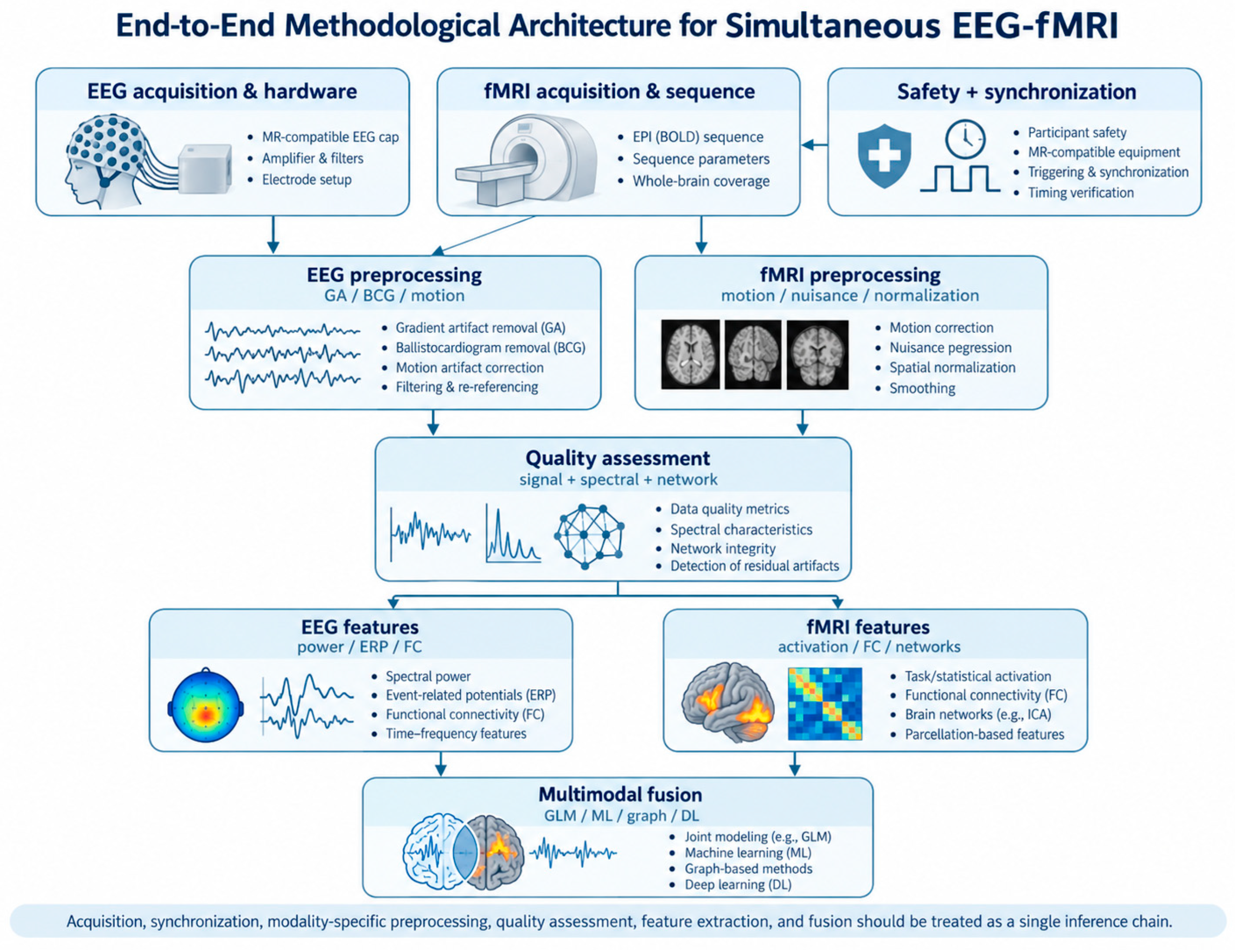
Figure 2.
Safety- and synchronization-aware architecture for simultaneous EEG-fMRI acquisition. Physical configuration, RF safety, cable routing, synchronization, and experimental timing are interdependent determinants of both signal quality and artifact morphology.
Figure 2.
Safety- and synchronization-aware architecture for simultaneous EEG-fMRI acquisition. Physical configuration, RF safety, cable routing, synchronization, and experimental timing are interdependent determinants of both signal quality and artifact morphology.
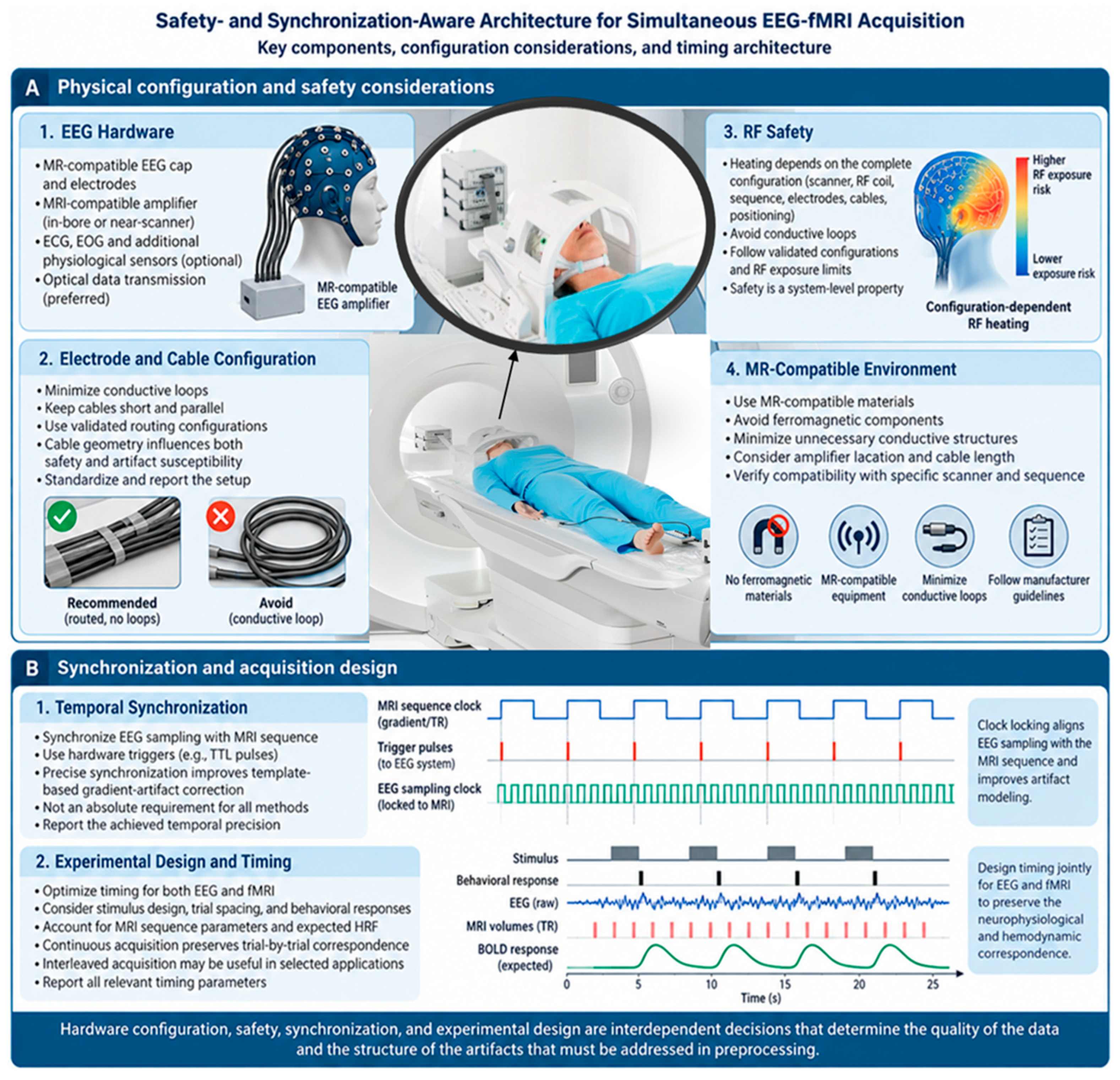
Figure 3.
Major sources of contamination in simultaneous EEG-fMRI. Gradient artifact is typically highly structured and sequence-locked, whereas BCG and motion-related contamination are more non-stationary and subject dependent. Physiological and environmental signals may additionally overlap with neural EEG, making artifact correction a problem of signal separation rather than simple noise suppression.
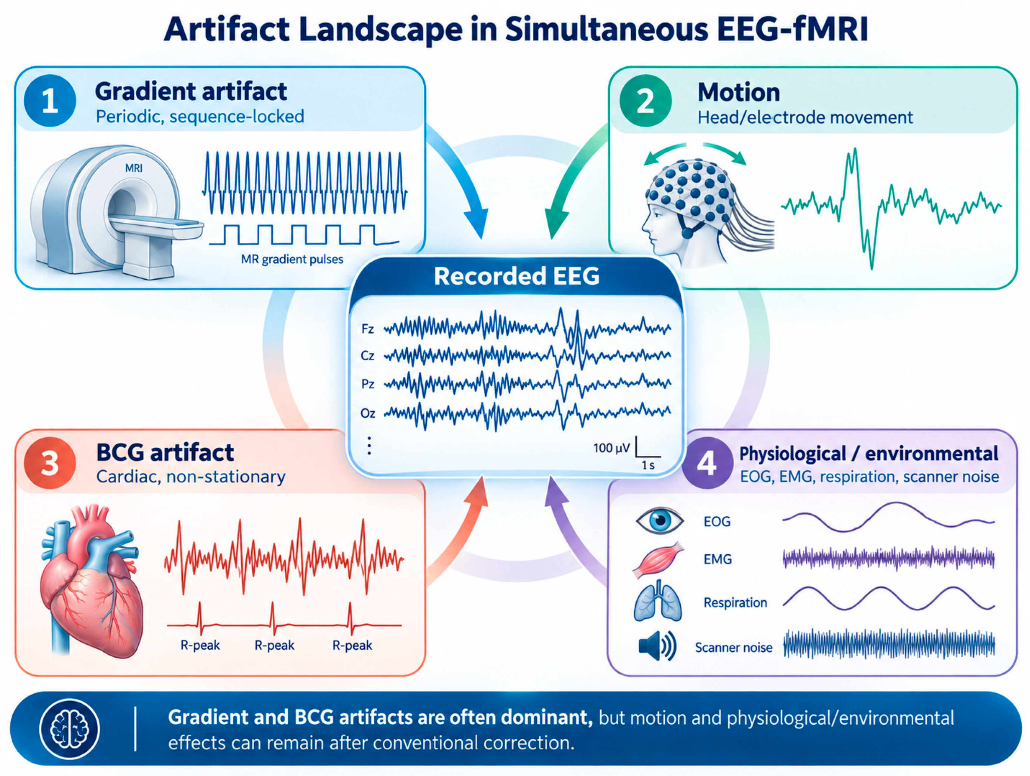
Figure 4.
Conceptual comparison of major gradient-artifact correction strategies. Each strategy introduces a different trade-off among artifact attenuation, model flexibility, neural-signal preservation, synchronization requirements, and generalizability.
Figure 4.
Conceptual comparison of major gradient-artifact correction strategies. Each strategy introduces a different trade-off among artifact attenuation, model flexibility, neural-signal preservation, synchronization requirements, and generalizability.
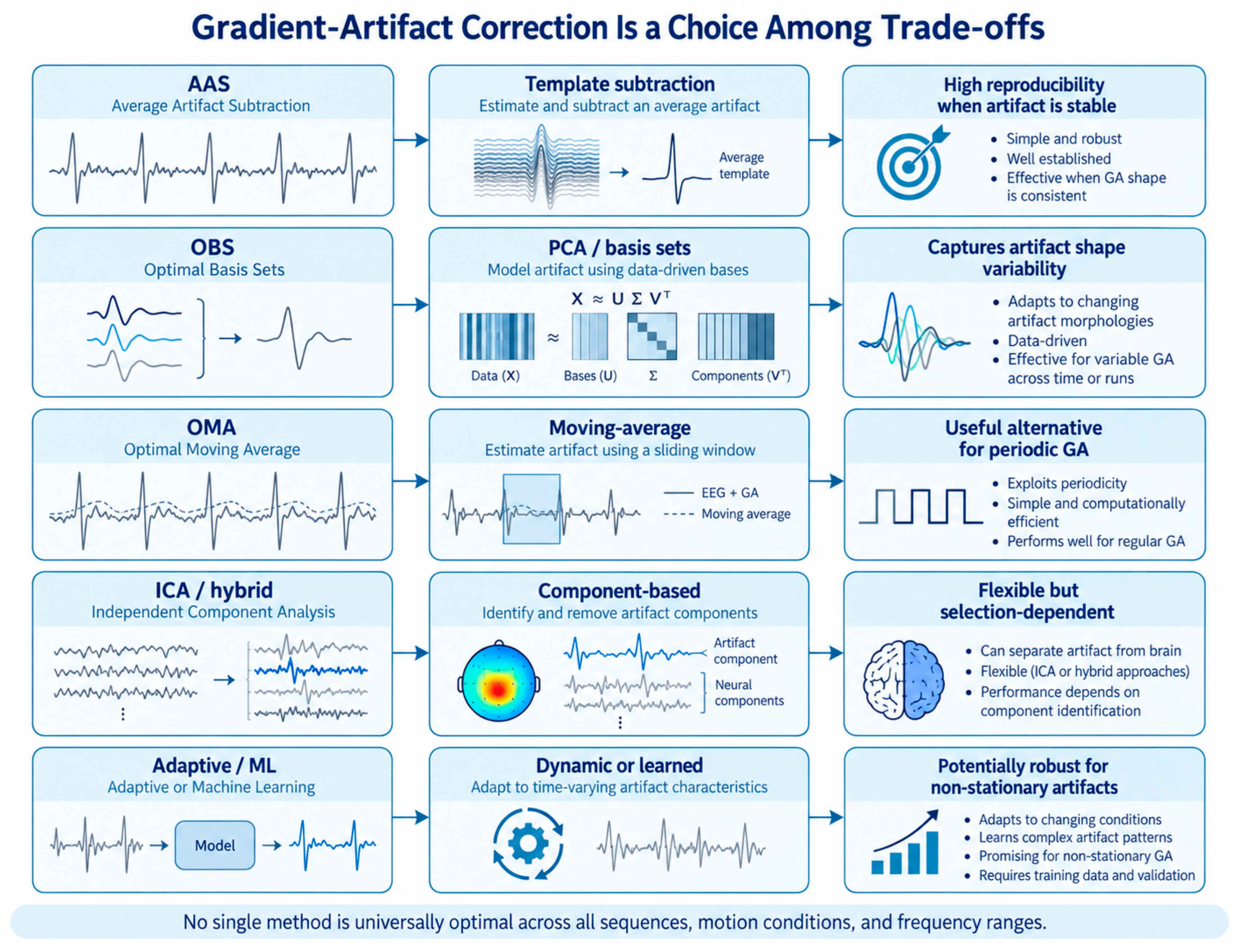
Figure 5.
Five-level validation framework for EEG-fMRI preprocessing. Artifact attenuation is necessary but not sufficient; correction should also preserve waveform, neurophysiology, network structure, and the intended scientific inference.
Figure 5.
Five-level validation framework for EEG-fMRI preprocessing. Artifact attenuation is necessary but not sufficient; correction should also preserve waveform, neurophysiology, network structure, and the intended scientific inference.
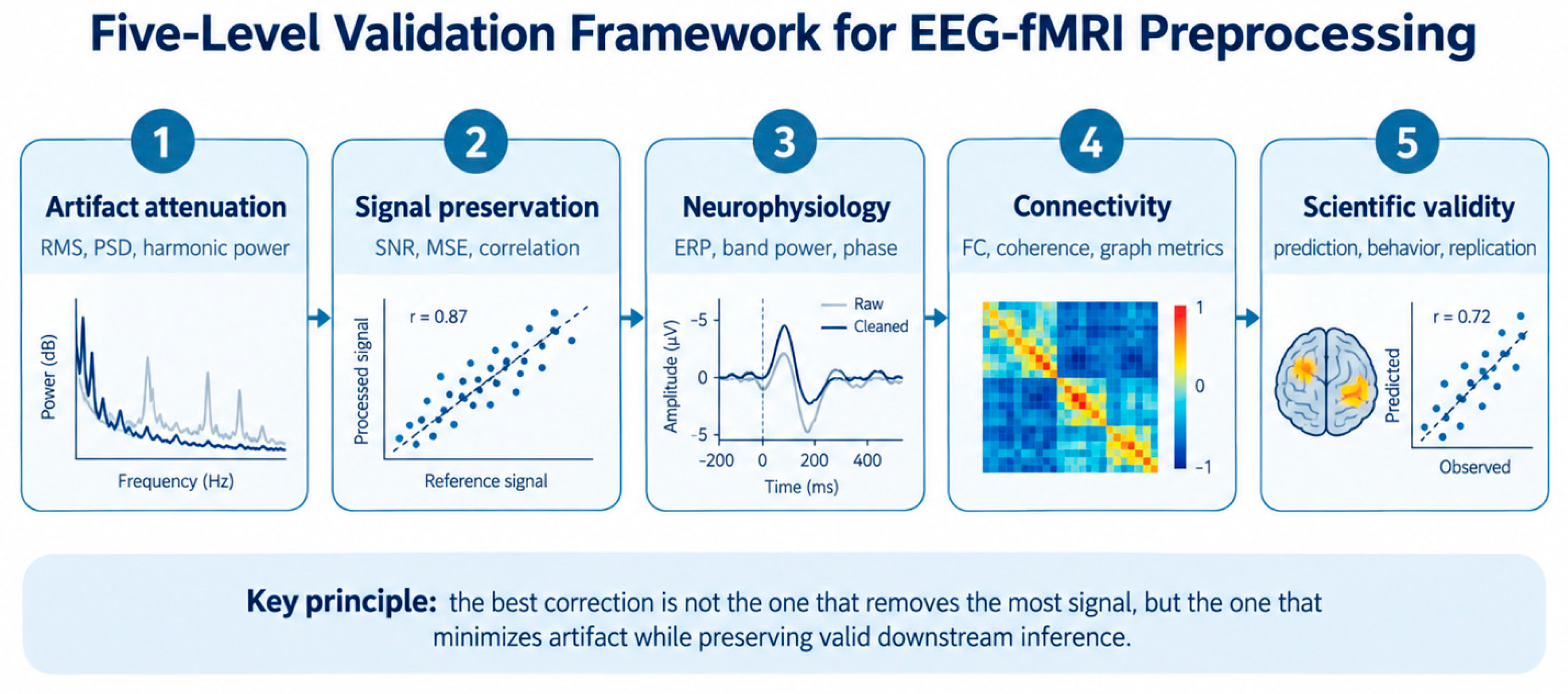
Figure 6.
Taxonomy of EEG-fMRI integration and data fusion. The field spans asymmetric EEG-informed or fMRI-informed analyses, symmetric/joint models, multivariate prediction, connectivity-level integration, and deep or graph-based representations.
Figure 6.
Taxonomy of EEG-fMRI integration and data fusion. The field spans asymmetric EEG-informed or fMRI-informed analyses, symmetric/joint models, multivariate prediction, connectivity-level integration, and deep or graph-based representations.
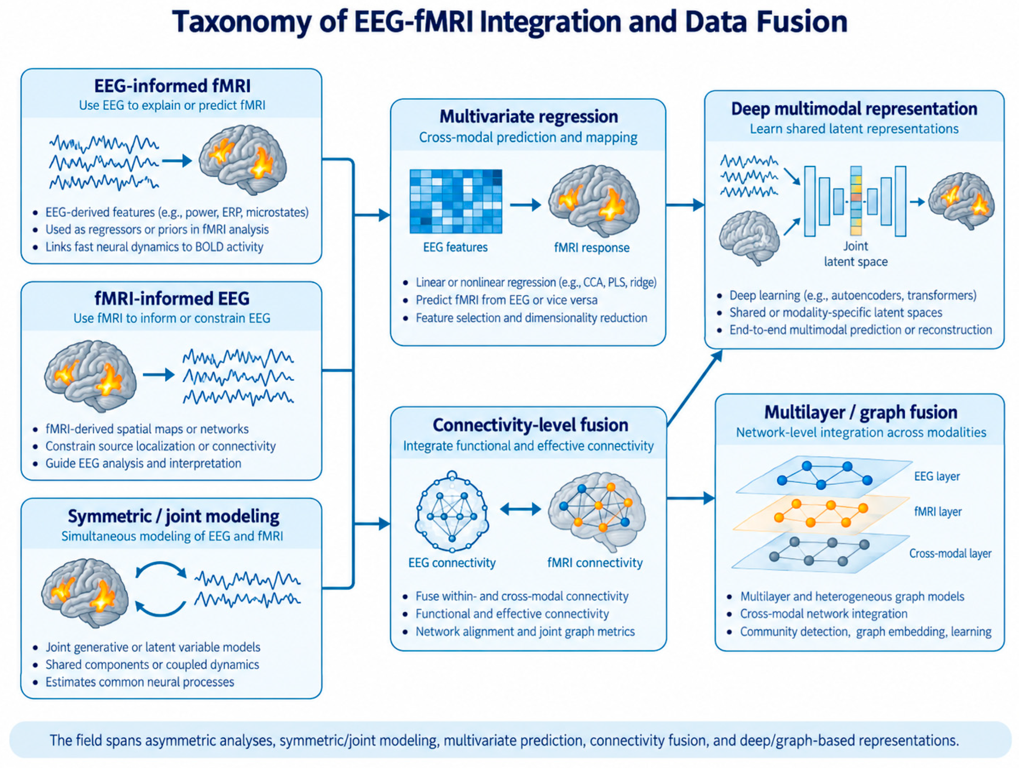

Table 1.
EEG preprocessing stages, quality-control targets, and downstream risks.
| Stage | Primary objective | Typical QC | Main risk if poorly designed |
|---|---|---|---|
| Raw-data QC | Verify signal and trigger integrity | Missing samples, saturation, bad channels, trigger counts | Acquisition errors misclassified as physiology |
| GA correction | Remove periodic scanner artifact | Residual harmonics, RMS/PSD, timing consistency | Neural high-frequency activity removed or residual GA retained |
| BCG correction | Reduce cardiac-related contamination | ECG association, morphology, spectral checks | Cardiac-related neural/source information removed |
| Channel/reference QC | Stabilize spatial covariance | Bad-channel statistics, reference sensitivity | Connectivity/source estimates distorted |
| Filtering | Suppress noise while preserving target band | Pre/post PSD, ERP and phase checks | Spectral or temporal distortion |
| Epoch QC | Remove unusable trials/segments | Rejected fraction and reason codes | Selection bias or contaminated trials retained |
| Feature extraction | Generate analysis-ready representation | ERP/power/FC stability and sensitivity analysis | Downstream inference inherits preprocessing bias |
Table 2.
fMRI preprocessing operations and cross-modal implications.
| Operation | Primary purpose | Key decision | Cross-modal implication |
|---|---|---|---|
| Initial-volume handling | Remove/model non-steady-state effects | Sequence-specific handling | Preserve EEG-fMRI timing after removal |
| Motion correction/censoring | Control displacement-related effects | Reference, interpolation, thresholds | Motion can also alter EEG artifact morphology |
| Distortion/registration | Improve anatomical localization | Fieldmap/topup and registration strategy | Improves EEG-to-fMRI ROI correspondence |
| Physiological denoising | Reduce cardiac/respiratory variance | Physio regressors, aCompCor, ICA | May remove variance coupled to EEG or behavior |
| Nuisance regression | Control confounds | Motion, WM/CSF, global/ICA components | Can alter FC and EEG-BOLD coupling |
| Temporal filtering | Control slow drift/high-frequency noise | Cutoffs based on design and FC target | Can change coupling with EEG rhythms |
| Spatial smoothing | Improve SNR/group inference | Kernel matched to resolution and target | Can blur cross-modal ROI correspondence |
| ROI extraction | Create modality-compatible nodes | Atlas, source mapping, node ordering | Essential for FC and graph fusion |
| Connectivity QC | Assess robustness | Motion sensitivity, alternate pipelines | Determines whether fusion is stable |
Table 3.
Fusion strategies, principal trade-offs, and recommended validation.
| Fusion level | Representation | Strength | Main limitation | Recommended validation |
|---|---|---|---|---|
| Early / feature-level | Concatenated EEG + fMRI features | Simple and transparent | Dimensional imbalance and scaling | Nested subject-wise CV |
| Intermediate / latent | Separate encoders + joint latent space | Preserves modality-specific structure | Architecture dependence | Held-out subjects + ablation |
| Late / decision-level | Separate predictions combined | Modular; tolerant of modality mismatch | May miss cross-modal interactions | Independent test set |
| Regression / covariance | Feature matrices | Interpretable multivariate coupling | Linear/regularization assumptions | LOSO or nested CV |
| Connectivity / network | FC matrices or multilayer graphs | Natural for network hypotheses | Sensitive to preprocessing and node mapping | Pipeline sensitivity + subject-wise CV |
| Deep / graph representation | Neural encoders on features/graphs | Nonlinear and topology-aware | Data hungry; harder to interpret | Strong baselines + external validation |
Table 4.
Minimum reporting information for reproducible simultaneous EEG-fMRI.
| Domain | Minimum information |
|---|---|
| Scanner | Manufacturer/model, field strength, RF coil, relevant hardware |
| Sequence | EPI type, TR, TE, voxel size, slice order, acceleration/multiband factor |
| EEG | System, channel count, sampling rate, reference, ground, electrode type, impedance |
| Synchronization | Trigger source, hardware/software synchronization, measured timing precision |
| Safety/setup | Lead routing, amplifier position, cable geometry, validated operating conditions |
| Artifact correction | GA and BCG methods/parameters; references; ICA/OBS details; rejected channels/segments |
| Filtering/reference | Filter type, cutoffs, phase characteristics, original and offline reference |
| fMRI denoising | Motion correction/censoring, nuisance regressors, physiological correction, smoothing |
| Fusion | Feature definitions, temporal alignment, HRF model, normalization, dimensionality reduction |
| Validation | Subject-wise split strategy, nested tuning, independent test set, sensitivity analyses |
| Reproducibility | Software versions, code availability, BIDS/data availability, correction/version history |
Disclaimer/Publisher’s Note: The statements, opinions and data contained in all publications are solely those of the individual author(s) and contributor(s) and not of MDPI and/or the editor(s). MDPI and/or the editor(s) disclaim responsibility for any injury to people or property resulting from any ideas, methods, instructions or products referred to in the content. |
© 2026 by the authors. Licensee MDPI, Basel, Switzerland. This article is an open access article distributed under the terms and conditions of the Creative Commons Attribution (CC BY) license (http://creativecommons.org/licenses/by/4.0/).
Copyright: This open access article is published under a Creative Commons CC BY 4.0 license, which permit the free download, distribution, and reuse, provided that the author and preprint are cited in any reuse.