

Submitted:
30 September 2026
Posted:
02 October 2026
You are already at the latest version
Abstract
Permanent magnet synchronous motor (PMSM) drives commonly use a mechanical position sensor, and position sensorless control removes this transducer by reconstructing rotor position and speed from electrical measurements. Fractional order operators have been introduced into observers, speed adaptation laws, position reconstruction loops, disturbance compensators, and feedback controllers to shape the estimation and regulation dynamics. This paper combines the operating characteristics of position sensorless PMSM drives and summarizes the application of fractional order methods in this field, including fractional order sliding mode observation, model reference adaptation, flux and back EMF estimation, and position reconstruction based on phase locked and frequency locked loops, as well as the interaction between fractional order controllers and estimated rotor feedback and the digital realization of non-integer order operators. The reviewed literature shows improvements in selected position error, speed response, and harmonic measures under specified machines, operating points, and baselines; however, component-level convergence does not generally establish stability of the complete output-feedback drive, back EMF methods retain an information limitation near standstill, and simultaneous changes to observers, controllers, and tuning procedures impede attribution to the fractional order element. Based on the current status, the development prospects for fractional order sensorless control are discussed, and the conditions under which a fractional-order design can be assessed reproducibly are identified.
Keywords:
permanent magnet synchronous motor
; position sensorless control
; fractional order observer
; rotor position estimation
; output feedback control
; digital implementation
1. Introduction
Permanent magnet synchronous motors (PMSMs) are used in high performance electric drives because control of the stator current vector permits precise electromagnetic-torque production [1,2]. In field-oriented control, this vector is resolved with respect to the rotor magnetic field, so the electrical rotor position is required for the coordinate transformation and rotor speed is required by the speed loop [3]. A position sensorless drive removes the mechanical position transducer but not these feedback variables. They must instead be reconstructed from measured electrical quantities and a motor model [4]. The central design problem is whether the reconstructed position and speed remain sufficiently accurate and stable over the operating range required by the application.
The electrical measurements do not contain rotor position as an isolated signal. In a surface-mounted PMSM (SPMSM), rotor position is inferred from the direction of a back-electromotive force (back EMF) or flux vector; in an interior PMSM (IPMSM), magnetic saliency can supply additional position dependent information [5]. The available information changes with speed and excitation. The magnitude of fundamental back EMF approaches zero as electrical speed falls, whereas saliency can be exploited near standstill only when the motor and applied excitation yield a detectable position dependent response [6,7]. The voltage used in an observer may also differ from the terminal voltage because of inverter dead time, device voltage drops, modulation, and sampling delay [8]. Consequently, observability and estimation accuracy cannot be attributed to an observer algorithm independently of the machine, signals, parameters, and operating point.
These physical constraints propagate into closed-loop control. An error in the estimated angle rotates the current vector used by the controller, changing the apparent direct- and quadrature-axis components and hence the torque-producing current. Speed estimation error alters the outer-loop feedback, while the controller changes the voltages and currents on which estimation depends. Low speed operation is particularly demanding for fundamental-model observers, and increasing their gain cannot restore position information absent from the measured signals under the stated SPMSM conditions [9]. Starting by rotor alignment or open-loop acceleration and switching later to observer feedback is therefore distinct from holding zero speed under sensorless feedback. At higher electrical frequencies, filtering, sampling, and computation delay become increasingly important. A proof for an isolated observer or controller consequently does not automatically apply to the implemented sensorless output-feedback drive.
Conventional sensorless methods address different parts of this chain. Current, back-EMF, and flux observers reconstruct electrical states or vectors, whereas an arctangent calculation, phase locked loop (PLL), or frequency-locked loop (FLL) converts vector information into rotor position and speed. Sliding-mode observation, model-reference adaptive estimation, Kalman-type filtering, and saliency-based injection differ in their information source, correction mechanism, parameter assumptions, and valid speed region. Filtering a sliding-mode injection can suppress ripple but introduces phase delay; integrating a voltage residual can produce flux drift; and a PLL can track an inaccurate phase if its input vector is biased. These limitations motivate changes to the dynamics of observation and reconstruction, while leaving the source of position information unchanged.
Fractional order differentiation and integration offer an additional means of shaping those dynamics [10]. Published PMSM designs place a non-integer-order operator in a sliding variable or observer injection [11,12], in a PLL or flux-related reconstruction loop [13,14], in speed adaptation [15,16], or in a controller and disturbance-compensation branch [17,18]. The location matters: an integer order back-EMF observer followed by a fractional-order PLL is not a fractional order state observer, and a fractional-order speed controller does not by itself change the rotor-state estimator. Moreover, Caputo, Riemann–Liouville, Grünwald–Letnikov, and conformable definitions are not interchangeable because their history, initialization, and realization properties differ [19]. A scientific account must identify the operator and the state equation or control law in which it appears before interpreting a reported result.
Xu et al. [1] reviewed sensorless control methods for AC motor drives, Xu et al. [2] overviewed the position sensorless technology for PMSM systems, and Volpato Filho et al. [8] surveyed observers for high speed sensorless PMSM drives. In parallel, Tepljakov et al. [20] surveyed the milestones of fractional order control and its industrialization, while Ajasa et al. [21] provided a taxonomy of sliding-mode control strategies for PMSM speed regulation. However, these reviews address the sensorless estimation chain and fractional-order design separately; none examines how a fractional order element acts on a specific block of the sensorless estimation and feedback chain, and which state or error dynamic it actually modifies. Several representative designs illustrate this coupling: Yao et al. [11] replaced the sliding surface, the injection filter, and the phase locked loop together, Huang et al. [12] modified both the sliding surface and the phase locked loop, and Wang et al. [4] inserted a fractional quasi-resonant compensation branch beside a flux observer. A reduction in angle error or an improved speed transient then demonstrates the combined configuration under its test conditions, not necessarily the isolated effect of the fractional order term. Similarly, sliding surface reachability, bounded current error, and local PLL stability concern different mathematical objects, and neither can be promoted to a full closed-loop stability claim unless the interconnection and the realized fractional order approximation are analyzed.
Figure 1 presents the content structure of this review. The PMSM model, the measurable electrical signals, the fractional order definitions, and the classification of fractional order sensorless schemes are provided in Section 2. Fractional order rotor state estimation methods, including sliding mode observation, model reference adaptation, flux and back EMF estimation, and position and speed reconstruction, are examined in Section 3. The interaction between fractional order controllers and estimated rotor feedback, together with the stability analysis of the interconnected output feedback drive, is presented in Section 4. The digital realization of fractional order operators and the closed loop validation evidence are analyzed in Section 5. The discussion, conclusions, and prospects for future research are elaborated in Section 6 and Section 7.
2. Sensorless PMSM Dynamics and Fractional Order Design Principles
The analysis of a fractional order design begins with the electrical information available for rotor-state reconstruction. The model fixes which quantity can be estimated; the location of the non-integer-order operator then determines which dynamics it can modify.
2.1. Rotor Position Information in PMSM Electrical Dynamics
For a sinusoidal PMSM represented in the rotor-oriented synchronous frame, a commonly used electrical model is
where vd,vq and id,iq are the stator voltages and currents, Rs is the stator resistance, Ld,Lq are the synchronous inductances, ψf is the permanent-magnet flux linkage, and ωe is the electrical angular speed. The electromagnetic torque and mechanical dynamics can be written as
with ωe = pωm and . Here, p, J, B, and TL denote the pole-pair number, inertia, viscous coefficient, and load torque, respectively. The saliency term vanishes under the ideal SPMSM approximation Ld = Lq, whereas it remains part of the IPMSM torque and voltage coupling when Ld ≠ Lq. Consequently, a proof or estimator derived under the SPMSM equality cannot be transferred to an IPMSM merely by changing a parameter table; the state dependence and the available position information may change [5,9,16].
The same electrical dynamics may be expressed in the stationary αβ frame as
and, under the ideal SPMSM model,
The stationary-frame form is useful for rotor state observation because the measured phase currents can be transformed into iα,iβ without using the unknown rotor angle, and the back-EMF or flux vector contains the angular information to be reconstructed. By contrast, a dq-frame observer must be checked for circular dependence: if the transformation or observer matrix uses the true θe or ωe, the claimed estimation error system is not directly implementable until those quantities are replaced by estimates and the resulting coupling terms are retained. This coupling affects several reported observer structures and cannot be removed only by stating that the analysis is performed in a rotating frame [9,12,22].
The model reveals at least three non-equivalent sources of rotor-position information. First, back EMF encodes θe through its vector direction, but its magnitude is proportional to |ωe| in the ideal SPMSM relation above. Second, the rotor-flux vector retains an angular direction, although voltage model reconstruction is sensitive to resistance error, voltage bias, integration drift, and initial conditions. Third, IPMSM structural saliency or saturation-induced saliency can create a position dependent response to an injected or switching-frequency excitation. The extended-EMF formulation provides one way to collect permanent-magnet excitation and reluctance-related terms into an observable quantity for IPMSM sensorless control [5]. These information channels must remain distinct: nonzero-speed back-EMF evidence does not establish standstill observability, and a zero-speed result based on detectable saliency does not validate a fundamental-wave back-EMF observer under the same condition [1,2,9].
The coordinate frames, voltage/back EMF vector diagrams, and observer vector relations that define the available rotor position information are shown in Figure 2.
The measured, commanded, reconstructed, and estimated signals must also be separated. Stator current is normally sampled, whereas the stator voltage supplied to an observer may be a voltage command, a duty cycle reconstruction, or a compensated estimate of the inverter output. Dead time, semiconductor voltage drops, current offset error, pulse-width-modulation harmonics, and computation delay then enter the observer as input or model errors rather than as abstract disturbances [8]. Back EMF, rotor flux, rotor angle, and speed are generally not direct measurements in a sensorless loop; they are successive estimates obtained from those electrical inputs. Accordingly, a study should report whether vs is measured or reconstructed, which frame is used, which parameters are assumed known, and which nonidealities are compensated. Without these declarations, two observers with formally similar equations may operate on materially different information.
The variable governed by the state or adaptation equation determines what an observer estimates. Current observers reconstruct electrical states; back EMF and flux observers reconstruct electromagnetic vectors; PLLs, FLLs, arctangent blocks, or model reference mechanisms convert those vectors or model errors into and ; parameter observers identify quantities such as resistance or inertia; and disturbance observers estimateTL, lumped uncertainty, or periodic error components. These variables are coupled, but they are not interchangeable. Zhao et al. [23] connected a sliding mode observer, a back EMF state observer, and a fractional order synchronous PLL in series in an effective-flux scheme, whereas Liu et al. [16] generated the speed adaptation error of a MRAS from the cross product of reference and adjustable model current errors. In another configuration, Wang et al. [4] compensated periodic position error through a fractional quasi-resonant extended state branch while a flux observer remained the primary position source. Calling all three structures “fractional order observers” would conceal which state is estimated and which subsystem actually contains the fractional dynamics.
2.2. From Electromagnetic State Estimation to Feedback Control
A complete sensorless estimation path can be represented as
The state observer and the reconstruction block solve different problems. An SMO may estimate theαβ back EMF, after which a low pass filter and phase compensation, anatan2 operation, or a PLL/FLL produces position and speed. A flux observer may similarly provide a vector whose phase is tracked by a PLL. Huang et al. [13] combined an integer order saturation function SMO with aPIr fractional order PLL, Huangfu et al. [24] cascaded an FO-STSMO with a DSOGI–FLL–CPLL chain, and Li et al. [14] connected an integer order leaky voltage model flux observer with an FO-PLL. The fractional order in the last two reconstruction examples does not retroactively change the differential order of the upstream state observer.
The reconstruction block introduces its own assumptions. An atan2 calculation requires two consistent orthogonal components and is affected by vector amplitude and filtering phase. A PLL uses a phase detector error and a loop filter, so claims based on a small angle linearization remain local unless nonlinear capture, amplitude variation, speed reversal, and saturation are also analyzed. An FLL estimates frequency from an oscillatory signal but still depends on signal amplitude, orthogonali(1)kai)ty, and sign conventions. Hence, a proof that an electrical state error reaches a sliding manifold does not by itself prove convergence of or ; the phase extraction dynamics must be included or bounded separately [11,12,13].
In field-oriented control, enters the Park and inverse Park transformations, while commonly closes the outer speed loop. If , then the currents used by the controller are rotated relative to the true rotor frame; even with exact current sampling, the apparent d- and q-axis components contain terms proportional to sinΔθe and cosΔθe. The angle error therefore perturbs flux and torque regulation, whereas speed estimation error modifies the outer loop tracking error. In direct torque control, the estimated flux sector and torque related quantities similarly affect switching decisions. The observer, reconstruction block, coordinate transformations, current regulator, speed controller, inverter, and plant consequently form an output feedback interconnection rather than independent modules [17,18,25].
The complete sensorless drive is therefore an output feedback interconnection rather than a set of independent modules, and representative architectures, from conventional field-oriented vector control with an inner current loop and SVPWM inverter to full order-observer structures feeding a common position/speed estimation stage, are shown in Figure 3.
This signal flow view supplies an operational test for sensorless feedback. During a claimed sensorless interval, the position or speed used by the transformations, switching logic, or feedback controller must come from the estimator rather than from a mechanical sensor. A plotted estimate alone is insufficient. The same rule applies to disturbance observers: estimating load torque may improve a speed controller, but it does not provide rotor position unless a separate rotor state estimation path is present. These distinctions are particularly important in composite fractional order systems, because a fractional controller can coexist with an integer order rotor observer and a separate disturbance observer. Module level stability results should therefore be attributed to their actual error variables; they do not automatically constitute a stability result for the complete implemented output feedback drive.
The presence of an encoder in an experimental rig is not, by itself, inconsistent with sensorless validation; its signal purpose is decisive. Three cases must be recorded separately. First, an encoder may provide the feedback variable used by the controller, in which case observer outputs are monitoring or comparison signals and the experiment does not demonstrate sensorless closed loop operation. Ilten [19] explicitly reports encoder speed feedback while the EEMF and conformable fractional order EEMF estimates do not enter the control feedback. Second, an encoder may be isolated from control and used only as ground truth for error calculation, as reported by Wang et al. [4]. Third, the drive may start with rotor alignment, open loop frequency ramping, or I–F control and later switch to estimated feedback. Huang et al. [12] switch after the drive reaches 600 r/min and satisfies an angular error condition, whereas Cheng et al. [26] use I–F acceleration to approximately 5000 r/min before observer feedback. These are valid stage specific architectures, but they do not demonstrate sensorless zero speed feedback during the starting interval.
2.3. Fractional Order Operators in Control Systems
For n − 1 < α < n, the left sided Riemann–Liouville (RL) fractional integral and Caputo derivative may be written as
The RL derivative instead applies an integer derivative after a fractional integral,
whereas the Grünwald–Letnikov form is defined through a weighted history sum,
These nonlocal operators explicitly depend on a lower terminal and past values. The Caputo form is often convenient when initial conditions are specified through integer-order derivatives, while RL or GL expressions can map naturally to convolutional numerical implementations. The choice is not a notation change: the initial terms, composition rules, and discrete realization depend on the definition [10,27].
The selected operator definition and its frequency characteristics shape the designed dynamics; the geometric interpretation of the fractional order derivative as a power law memory kernel, the isodamping property of fractional controllers, and the Bode responses of rational approximations are shown in Figure 4.
A conformable derivative is mathematically different. For differentiable f and 0 < α ≤ 1, a common definition reduces to
It is local and does not generate the power law history convolution present in the preceding nonlocal definitions. Ilten [19] employs a conformable fractional order EEMF formulation; the reviewed equation therefore cannot be interpreted automatically as evidence of long-memory dynamics. For the same reason, a non-integer algebraic power such as |e|p/qsgn(e) in a terminal sliding surface is not a fractional derivative or integral. A study belongs to fractional order control only when an operator such as Dα or Iα is actually defined and used in the dynamics or control law.
The lower terminal t0, the prehistory of the signal, and the initialization of the numerical realization are part of a fractional order model. Identities such as DαIαf = f or the cancellation of DαD−α require compatible definitions and initial history conditions; they should not be used as unconditional algebraic cancellation rules. This issue appears directly in a close reading of a PMSM fractional sliding mode design whose D0.8D−0.8 simplification was not accompanied by a definition or initial history statement [28]. Likewise, reporting a fractional sliding surface without its lower terminal, order, and approximation parameters prevents exact reconstruction of the implemented algorithm [11,16].
Dimensional consistency imposes a related constraint. If x has physical unit [x], then Dαx has unit [x] s−α under the usual time based definition. Replacing dx/dt by Dαx while retaining every integer-order coefficient unchanged generally alters the dimensions of the equation unless a characteristic time or appropriately dimensioned coefficient is introduced. An assumed fractional PMSM current model therefore requires more than selecting 0 < α < 1: the order should be reported, the coefficients should be dimensionally consistent, and a physical or identification argument should explain whether the order represents plant memory or merely a design degree of freedom. Zhou et al. [29] illustrate this boundary because its proposed fractional current model does not report the order and retains ordinary inductance units without an accompanying dimensional or identification treatment. Until such evidence is available, a fractional plant model should not be treated as interchangeable with an integer order PMSM plus a fractional controller.
Real time control cannot implement an ideal infinite memory operator directly. Time domain implementations approximate the history convolution using sampled weights and usually truncate or compress the memory. Frequency domain implementations replace sα by a rational transfer function over a selected band, creating additional poles, zeros, and states. The implementation is therefore defined not only by α, but also by the approximation family, frequency band, rational order or memory length, sampling period, initialization, coefficient precision, and scheduling budget [10]. Different approximations can preserve stability and transient behavior differently near a stability boundary, so they cannot be ranked independently of the plant and design band [30].
Published realizations differ substantially in what can be reconstructed. Li et al. [14] approximate s−0.6 by a seventh order Oustaloup filter over 10−4–104 rad/s, but do not fully specify the subsequent discretization and coefficient implementation. Ahmed et al. [27] use product trapezoidal history convolution for an RL integral, while step size, memory truncation, and computational cost remain insufficiently described. By contrast, Wang et al. [4] report a 13 state fractional quasi-resonant ESO executed at 16 kHz with a component time of 9.85 μs, compared with 3.79 μs for an ESO and 5.43 μs for an integer-order quasi-resonant ESO on the stated processor. The last result demonstrates feasibility on that platform, not a worst case bound for the complete control task.
2.4. Classification of Fractional Order Sensorless Schemes
The primary classification adopted in this review is the physical and mathematical location of the fractional operator. Five locations are distinguished: (i) the plant or observer state equation, including fractional error dynamics and fractional sliding surfaces that directly determine state estimation; (ii) the position/speed reconstruction block, such as an FO-PLL or FO-FLL applied after an integer order back EMF or flux observer; (iii) an MRAS parameter or speed adaptation law; (iv) the current, speed, torque, or position controller while the rotor observer remains integer order; and (v) a disturbance or periodic-error compensation branch coupled to a primary rotor state observer. This axis resolves the apparent conflict between papers that use the same broad label but place Dα or Iα in different equations [13]. Table 1 applies this rule to representative architectures.
The five locations of the fractional order operator, and representative schemes in each class ranging from fractional operators inside the observer and the model reference adaptation law to fractional order controllers and disturbance compensation branches, are illustrated in Figure 5.
The secondary axis records the estimated quantity and the equation that corrects it. Electrical state observers use current error to reconstruct current, back EMF, or flux; kinematic reconstruction blocks convert an electromagnetic vector into angle and speed; MRAS structures compare reference and adjustable models to adapt speed or a parameter; disturbance observers reconstruct load torque, lumped uncertainty, or periodic error; and controller states act on tracking errors without necessarily estimating rotor states.
This record prevents two common category errors. A load torque estimate is not a rotor position estimate, even if it improves speed regulation; and a PLL that tracks the phase of an estimated flux vector is not the flux observer itself. It also exposes invalid signal mappings: a PLL driven by inverter terminal voltage phase cannot be assumed to produce rotor electrical position unless the voltage to rotor angle relationship is derived under stated machine and operating conditions [31].
A fractional order state observer is identified by a defined non-integer order operator in its state equation, correction law, sliding variable, or estimation error dynamics. The sliding-mode designs of Huang et al. [12], Zhou et al. [29], and Huangfu et al. [24] satisfy this structural condition in different ways; the mathematical scope of each result still depends on the stated operator and proof assumptions. In contrast, Huang et al. [13] and Li et al. [14] retain integer order electromagnetic state observers and place the fractional term in the PLL. Niu et al. [15] include Caputo adaptation in a voltage control component while their speed MRAO uses PI adaptation. Xiao et al. [18] and Wang et al. [25] combine fractional controllers with integer order rotor observers. In Wang et al. [4], a fractional quasi-resonant extended state branch compensates position error downstream of a flux observer. The estimated state and operator location, rather than a common label, determine which estimation error equation can be analyzed.

Table 1.
Classification of representative fractional order structures in PMSM rotor position and speed estimation chains.
Table 1.
Classification of representative fractional order structures in PMSM rotor position and speed estimation chains.
| Sources | Motor | Information source | Observer or estimator | Fractional order location | Estimated quantities | Feedback use | Principal boundary |
|---|---|---|---|---|---|---|---|
| [11] | SPMSM | current and voltage to back EMF | FONTSMO plus adaptive back EMF filter | sliding surface and FO PLL | back EMF position speed | reported sensorless feedback | RL definition and implementation parameters incomplete; stability claims conditional |
| [12] | PMSM | current and voltage to back EMF | fractional integral SMO | sliding surface and FO PLL | back EMF position speed | I-F start then observer feedback | switch at 600 r/min; ideal proof omits realization states |
| [29] | PMSM | assumed fractional current model | FOTSM back EMF observer | plant or observer model and injection | back EMF position speed | reported sensorless feedback | fractional order and dimensional consistency not established |
| [23] | PMSM | effective flux equivalent back EMF | STW SMO plus back EMF state observer plus FO SPLL | FO PLL only in reconstruction | back EMF position speed | reported sensorless feedback | effective-flux derivative approximation and printed observer equations require caution |
| [13] | PMSM | alpha beta back EMF | integer order saturation SMO | PI^r FO PLL only | back EMF position speed | reported sensorless feedback | r=1 gives integer-order PLL; phase-compensation path unclear |
| [19] | PMSM | extended back EMF | conformable FO EEMF observer | conformable derivative in observer | EEMF and comparison signals | encoder speed feedback | observer output not used for control feedback; conformable derivative is local |
| [32] | IPMSM and SPMSM | effective flux | VGSMO plus FO PLL | FO PLL only in reconstruction | flux position speed | reported sensorless feedback | printed error dynamics and proof contain unresolved consistency issues |
| [24] | PMSM | current error to back EMF | FO STSMO plus DSOGI FLL CPLL | fractional order in observer injection or surface | back EMF position speed | reported mid high speed sensorless feedback | model/order and proof equations require qualification |
| [14] | SPMSM | voltage model flux | integer order leaky flux observer | FO PLL only | permanent magnet flux position speed | reported sensorless feedback | filter causes amplitude/phase error; digital realization not fully reported |
| [15] | PMSM | current model MRAS | MRAO with PI speed adaptation | Caputo adaptation in voltage controller not speed observer | speed and position | reported sensorless feedback | parameter-adaptation proof does not establish all parameter convergence |
| [22] | PMSM | dq back EMF | integer order NFTSMO | FO SPLL only | back EMF position speed | reported sensorless feedback | dq model uses unknown speed/angle and proof conditions are incomplete |
| [16] | SPMSM | dq current model error | MRAS observer | fractional integral sliding surface and speed adaptation | speed then position | reported sensorless feedback | operator definition initial conditions and realization incomplete |
| [4] | PMSM | flux observer position error and current error | flux observer plus FOQR ESO | fractional quasi resonant compensation branch | position error compensation | estimated position speed feedback encoder for evaluation | sixth-harmonic model is specific approximation; implementation evidence is platform-specific |
Table 1 is a structural evidence map, not a performance ranking. It shows that apparently similar “fractional order sensorless” systems may modify different equations and may even differ in whether the estimated state enters feedback. The resulting classification links each architecture to its estimated state and error dynamics.
3. Fractional Order Methods for Rotor State Estimation
The methods considered below differ first in the electrical quantity reconstructed from voltage and current and then in the mechanism used to obtain rotor position and speed. Keeping these two stages separate avoids assigning the dynamics of a downstream PLL to the upstream observer.
3.1. Sliding Mode Observation of Back EMF
For an SPMSM represented in the stationary frame, a common observer starts from the current model
and constructs an estimated current system in which an injection vector z replaces the unknown back EMF. With , the ideal error dynamics take the form
Once the sliding motion is established, the equivalent value of z can be associated with eαβ, usually after filtering or continuous-injection reconstruction. This architecture underlies conventional, terminal, nonsingular terminal, and super-twisting sliding mode observers. In the reviewed fractional order variants, the non-integer operator has been placed in the sliding variable, the injection dynamics, an assumed fractional plant/observer model, or the downstream PLL; these placements generate different error systems and should not be combined into one observer class merely because all use a switching term [11,12,23].
A representative fractional integral sliding variable may be written schematically as
Representative fractional order sliding mode observer structures, including fractional order non-singular terminal, super-twisting, and full order terminal designs together with their downstream phase locked reconstruction, are shown in Figure 6.
whereas other designs embed or in terminal powers or in an auxiliary injection state. The added order parameter changes the frequency dependent weighting of the estimation error and can reshape the transient between high frequency measurement disturbances and lower frequency tracking errors. However, the mathematical object being modified must be stated exactly. A fractional order sliding variable built on an integer-order current model is not equivalent to replacing the PMSM state equation by a fractional differential equation; similarly, an integer order observer followed by an FO-PLL remains an integer order state observer with a fractional order position/speed estimator. The latter distinction is especially important because the physical interpretation, initial condition requirements, and dimensional consistency of a fractional plant model are much stronger claims than the use of a fractional element as a design compensator.
The discontinuous injection that enforces a sliding motion also excites switching ripple, measurement noise, and unmodeled inverter dynamics. Low pass filtering of the equivalent injection is the simplest reconstruction route, but its phase lag must then be compensated in the angle estimator. To reduce the visible ripple, Yao et al. [11] attached an adaptive back EMF filter to a fractional order nonsingular terminal sliding mode observer, Huang et al. [12] smoothed the equivalent injection through a fractional integral sliding surface, and Zhao et al. [23] replaced the sign injection by a boundary-layer approximation inside a super-twisting observer. These mechanisms are not interchangeable: a boundary layer generally changes exact sliding into practical convergence, a low pass filter trades attenuation for phase delay, and a super-twisting structure requires boundedness conditions on the matched perturbation and its derivative. A smoother back EMF or smaller angular ripple therefore supports the behavior of the complete implemented chain under the tested conditions, but it does not identify whether the improvement arose from the fractional sliding variable, the continuous injection, the filter, the PLL, or their joint retuning.
For a sliding variable s, a Lyapunov candidate V = 1/2sTs establishes reachability only when its derivative is negative under implementable gain bounds for the actual estimation error system. Reaching s = 0 is distinct from convergence of current, back EMF, position, and speed errors. Equivalent injection reconstruction also presupposes the sliding regime, whereas fractional derivative composition requires a specified operator, lower terminal, and initial history. A proof for an ideal continuous time model does not encompass a rational approximation, boundary layer regularization, sample and hold, or numerical recurrence unless their states and errors are included. Several designs leave one or more of these conditions unresolved, so their reported operation supports the particular configurations tested but not a general finite time theorem for the complete sampled data sensorless drive.
Related observer analyses illustrate why the proven variable must be stated. In Qiao et al. [33], a quadratic argument dissipates back EMF error after continuous sigmoid injection, but speed error convergence needs an additional invariance or excitation argument. Wei et al. [34] introduce fractional action in an integral sliding observer without deriving the claimed finite time property from explicit disturbance bounds. Zhong et al. [35] establish conditions for uncertain fractional order nonlinear systems; applying them to a PMSM observer requires verification of the operator, regularity, and uncertainty hypotheses. These results offer possible design tools, but a theorem cannot be transferred to a different realized observer merely because the methods share a name.
3.2. Model Reference Adaptation of Rotor Speed
Model reference adaptive systems estimate speed by comparing a reference model constructed from measured variables with an adjustable model that contains the estimated electrical speed. For a current model MRAS, a scalar adaptation error is often formed from the cross coupled current model mismatch, for example or a sign equivalent expression determined by the selected model convention. A PI, sliding mode, or fractional order adaptation law then updates , after which is obtained by integration. In Niu et al. [15] and Liu et al. [16], fractional order elements occur in different locations: one design combines an MRAO with fractional order PI regulators or adaptation, whereas the other introduces a fractional integral sliding term into a second order sliding speed adaptation law. Both are adaptive speed estimation arrangements, but they do not share the same fractional order state equation.
Adaptive observer analyses commonly select a quadratic current error function and design the speed law to cancel a cross term. This can show non-increase of the chosen function under the printed nominal model. However, a negative semidefinite derivative does not alone establish convergence of the speed error. Such a conclusion additionally requires an invariant set or excitation argument, consistency between the law used in the proof and the implemented PI or sliding algorithm, and retention of the coupling caused by using in the coordinate transformations. For fractional adaptation, the admissible derivative inequality and composition of Dρ and Iρ also depend on the chosen fractional definition and initial conditions. The reviewed MRAS studies provide useful construction principles, yet their mathematical results should be reported as conditional subsystem guarantees rather than proof of the complete sensorless output feedback loop [15,16].
MRAS changes the route by which rotor speed is inferred, but it does not remove the information requirement. If the reference and adjustable models become weakly distinguishable, the current error can remain small while the speed or an uncertain parameter is not uniquely identified. Stator resistance variation is especially influential at low speed, where the resistive voltage drop is comparable with the speed dependent voltage term; integration of a biased speed estimate then produces angle drift. Parameter convergence therefore requires sufficient excitation and identifiability, not only bounded tracking error. The existing results demonstrate tracking for specified speed and load profiles, including selected low nonzero speeds in simulation, but they do not establish a common excitation condition or a zero-speed position observability result across PMSM types.
Multi-parameter adaptive schemes make this limitation more explicit. Sun et al. [36] update speed, stator resistance, and permanent magnet flux through coupled estimation loops, but the separate derivations that cancel one error while holding the others fixed do not establish simultaneous parameter convergence. Kivanc et al. [37] combine feedforward voltage estimation with MRAS parameter updating and evaluates closed loop margins at a specified low speed, full load operating point. Shi et al. [38] similarly reports that estimating resistance and flux with one adaptive structure can lead to incorrect convergence and therefore separates the unknowns between estimators. These results support online compensation for selected parameter variations, while also showing that joint identifiability and coupled stability must be proved for the complete estimator.
3.3. Flux Observation and Error Compensation
Back EMF observers reconstruct a vector whose direction is tied to rotor position and whose magnitude is proportional to speed under the ideal SPMSM model. Flux observers instead integrate the voltage residual vαβ − Rsiαβ and subtract the inductive flux, allowing the permanent magnet or active flux vector to be used for angle calculation. Active flux formulations can extend the vector interpretation to salient machines by incorporating the reluctance related current term. The attraction of these methods is that they use stationary frame voltage and current signals without requiring the unknown angle in the primary reconstruction. Their limitations follow from the same signal path: voltage offsets cause integration drift, resistance error dominates at low frequency, leakage or high pass correction introduces magnitude and phase distortion, and active flux equivalence depends on the assumed machine and operating conditions.
An extended state observer augments the nominal state with a lumped disturbance representing parameter error, unmodeled dynamics, or a structured periodic component. In a position error compensator, for example, the measured or reconstructed error y can be modeled as the sum of a slowly varying term and a harmonic component, and an augmented observer estimates these components for correction. The FOQR-ESO of Wang et al. [4] follows this route: the primary rotor position comes from a flux observer, while a fractional quasi-resonant extended state is driven by a common current error signal to compensate the dominant periodic position error. It is therefore a fractional order error-correction observer, not the primary source of rotor position. This distinction matters when interpreting both stability and performance: attenuation of a selected harmonic does not prove convergence of the upstream flux observer, and the augmented states increase implementation order and computation.
Dead time, voltage drops, current distortion, and model mismatch generate periodic estimation errors whose dominant order depends on the reference frame. In Wang et al. [4], fifth- and seventh-order inverter-related harmonics are represented primarily as a sixth order periodic disturbance in the synchronous frame, motivating an integer- or fractional-order quasi-resonant correction. This frequency selective formulation can raise the loop gain around the targeted disturbance frequency without uniformly increasing broadband observer gain. However, rotor speed changes move the disturbance frequency; the resonant dynamics must then be scheduled or remain sufficiently robust to detuning. Moreover, the same study reports both lower aggregate IAE at its tested steady speeds and greater sensitivity at some low frequency components or during a deceleration transient. The evidence consequently supports conditional harmonic error reduction, not uniform improvement over every frequency and transient [4].
Related compensation studies show several alternative realizations. Wu et al. [39] use frequency adaptive delay signal cancellation and fractional sample interpolation to place zeros at selected position error harmonics. Wang et al. [40] and Wang et al. [41] use adaptive notch or recursive least squares filtering to reduce fifth- and seventh-order back EMF components and their associated position errors. Liu et al. [42] combine ESO based current reconstruction with fractional order phase compensation in repetitive control for an LC filtered high speed drive. These methods confirm that harmonic attenuation may be achieved by adaptive filtering, delay cancellation, repetitive control, or resonant observation; only some contain fractional calculus operators, and each must therefore be classified by its actual compensator equation rather than grouped as a fractional observer.
A separate caution arises for conformable fractional order EEMF observation. The conformable derivative used in Ilten [19] is locally representable as a time varying scaling of an ordinary derivative under its stated definition, and its stated injection and Lyapunov cross term relations remain difficult to reconcile. More importantly for classification, the experiments retain encoder speed feedback while comparing estimated quantities. They can inform the behavior of the observer component, but they do not constitute a sensorless closed loop validation. This is not a judgment that the observer is ineffective; it fixes the level of claim supported by the reported signal path [19].
3.4. Position and Speed Reconstruction
Once a rotating back EMF or flux vector is available, direct arctangent calculation gives after the model dependent phase convention. A PLL instead constructs a phase error, filters it, and integrates the estimated frequency:
Replacing the loop filter by a fractional compensator such as CPLL(s) = kp + kis−λ adds a slope and phase-shaping parameter. This can improve a selected trade-off among tracking, phase lag, and noise attenuation. Yet the often-used linear model is local, and its gain depends on normalization and the magnitude of the observed vector. A transfer-function tuning argument must therefore be distinguished from global angle-error convergence and from stability of the upstream observer [11,12,13].
When the observed signal is distorted or does not arrive as an accurately orthogonal pair, the in phase and quadrature components required by the phase detector are generated by auxiliary blocks such as a second-order generalized integrator, a frequency-locked loop, a resonant unit, or a quadrature PLL. These blocks reject selected harmonics and estimate frequency simultaneously, at the cost of additional dynamic states, so their reported benefit holds only when the bandwidths of the observer, the orthogonal-signal generator, and the outer control loops are sufficiently separated. A stable polynomial of an isolated small-signal block is useful design evidence, but it does not cover the nonlinear, time-varying interconnection in which the input amplitude approaches zero or the estimated frequency schedules the filter.
Results for integer-order position reconstruction clarify which difficulties arise independently of fractional calculus. Wang et al. [43] analyze high-order sliding back-EMF observation under approximately constant speed, leaving the observer–QPLL interconnection outside the proof. Xu et al. [44] report low-speed loaded operation with a nonlinear ESO but not zero-speed self-starting, while Andreescu et al. [45] require initialization when transferring between signal injection and flux observation. Linearized adaptive-observer poles can depend on saliency and torque direction [46]; local exponential speed tracking can require persistent excitation [47]. Direct-integration observers provide yet another reconstruction route [48]. Across these architectures, excitation, local operating region, phase extraction, and feedback coupling govern the interpretation of a rotor-state estimate.
Position reconstruction must also preserve the model-specific angular offset, compensate filter-induced phase lag, handle amplitude variation, and determine the sign of speed. An atan2 operation avoids the quadrant ambiguity of a single argument arctangent, whereas normalized phase detectors reduce, but do not eliminate, the dependence on vector magnitude. At low speed, division by a small magnitude amplifies noise, and direct differentiation of the angle amplifies quantization and phase jumps; PLL/FLL dynamics provide filtered speed estimates but introduce transient lag and possible direction ambiguity around zero crossing. Because these choices change the meaning of the reconstructed angle, the reviewed studies differ in how the vector convention, phase compensation, normalization rule, initial alignment, and reversal logic are handled, and without those details a visually smooth angle trace cannot establish robust signed speed estimation.
3.5. Operating Range Constraints of Rotor-State Estimators
Table 2 compares the reviewed core methods by the variable reconstructed before angle extraction, the measured signals, the location of the fractional operator, the error used for correction, and the scope of the mathematical analysis. Three structural observations follow. First, current-error sliding observers estimate an equivalent back-EMF injection, flux observers integrate a voltage residual or reconstruct active flux, and MRAS methods adapt speed from a model mismatch; these information sources respond differently to resistance error, voltage uncertainty, and excitation. Second, placing the fractional operator in a PLL changes the position/speed estimator, not the upstream state observer. Third, a compensator that estimates a periodic position error should not be presented as the sole rotor-position observer. These distinctions are prerequisites for comparison because they determine both the available information and the state to which a proof applies.
No method suppresses all error sources through the fractional order alone. Increasing observer or PLL gain can accelerate tracking but transmit switching ripple and measurement noise. Flux integration reduces reliance on differentiation but accumulates voltage and resistance errors. Adaptive models can accommodate selected parameter uncertainty but require excitation and a correct reference/adjustable-model relation. Resonant correction attenuates modeled periodic components but is sensitive to frequency mismatch, while high-order sliding injection requires disturbance regularity and implementable gain bounds. Fractional-order elements provide an additional frequency-shaping variable within each compromise; they do not remove the compromise. Therefore, robustness claims should name the varied parameters, noise model, inverter nonlinearity, saturation, and bandwidth, and should not be inferred from a single load step [4,17,18].
Sampling delay is another identifiable error source rather than a generic uncertainty. Gong et al. [49] use double sampling compensation in a continuous injection SMO and reports a modest reduction in position error and back-EMF distortion under its tested conditions. The result illustrates an important comparison rule: an observed improvement obtained after delay compensation should be attributed to the compensated sampled-data observer, not to the switching function or observer order alone [49].
The decisive boundary for back EMF based position estimation is structural: under the ideal SPMSM relation ||e||=|ωe|ψf, the signal used to define the rotor angle vanishes as ωe → 0. Fractional filtering can improve phase and noise behavior when a usable vector exists, but it cannot by itself create missing position information at standstill. Existing studies accordingly use pre-alignment, I–F starting, switching at a nonzero speed, flux or saliency information, or evaluate only selected nonzero points. For example, one FO-SMO study activates observer feedback only above 600 r/min, while the FOQR-ESO study reaches 300 r/min, 15% of its rated speed; a separate optimized MRAS simulation reports 10 r/min under ideal no-load conditions. These results describe different tasks and do not define a common low-speed threshold.
Reversal adds the need to preserve the speed sign and to manage the interval in which the back EMF vector becomes small, whereas high speed operation poses a different problem: voltage saturation, sampling delay, discrete observer bandwidth, and field-weakening alter the model and the available control margin. Hardware evidence at selected speeds confirms that several structures can close the loop over their reported ranges, but it does not automatically establish zero speed holding, seamless cross-zero reversal, or the complete field-weakening range. Method selection should therefore start from the required information source and operating region, then examine model uncertainty, mathematical guarantees, discrete time realization, and available computation; once the estimate enters feedback, these component level properties become coupled.
4. Fractional Order Control with Estimated Rotor Feedback
When estimated position and speed enter the coordinate transformations and feedback laws, control and estimation form a coupled dynamical system. The classification therefore turns from observer type to the actual placement of fractional order elements and the stability property established for the interconnected drive.
4.1. Fractional Order Controllers with Conventional Rotor State Observers
The first architecture retains an integer order rotor state observer while inserting non-integer dynamics in a speed, position, current, or torque controller. Nicola et al. [17] designed fractional order and fractal dimension sliding mode controllers within a direct-torque control sensorless scheme, Nicola et al. [51] paired a fractional order sliding-mode outer loop with an integer order extended Kalman filter, Niu et al. [15] introduced fractional-order action into a model reference adaptive speed loop, Xiao et al. [18] combined a fractional-order integral sliding-mode speed controller with a cascaded sliding-mode and high-gain observer, and Wang et al. [25] retained an integer-order current-model MRAS under a fractional speed controller. In these systems, “fractional-order sensorless control” correctly describes the complete control scheme, but “fractional-order observer” does not describe the state estimator, because the fractional elements occur in control or parameter-adaptation blocks while the primary state-observer equations remain integer order. This classification determines which state and estimation-error equation can be associated with the fractional order [15,17,18].
The nominal controller is usually derived under true or perfectly known rotor variables. With sensorless feedback, the Park transformation instead uses , so the transformed currents contain angle-error-dependent coupling. For small ,
but the exact nonlinear relation, saturation, and current-loop dynamics remain part of the plant seen by the outer controller. Consequently, a Lyapunov proof that substitutes the true speed or load torque into a fractional sliding law does not establish the implemented sensorless system if the realizable law uses estimates, filters, or unavailable derivatives. Several controller observer configurations retain precisely this gap: the controller or observer proof treats a reduced nominal error system while the actual feedback path contains angle estimation, numerical differentiation, PI replacement, or unreported signals [17,18,25].
These configurations nevertheless show that fractional controllers can operate with conventional state observers over the reported conditions. Xiao et al. [18] combined an FO integral sliding-mode speed controller with an integer order ASMO and an extended high-gain observer and reported a lower speed error standard deviation than their selected PID and integer-order sliding baselines in a load-switching test; the maximum absolute speed deviation changed much less, and encoder-referenced rotor-state errors were not reported. Nicola et al. [51] simulated an FO sliding controller with an EKF and reported selected speed and position responses, but omitted sampling, covariance identification, and a local observability analysis. These two designs demonstrate architectural feasibility under their stated conditions; neither isolates an improvement in observer accuracy caused by fractional control [18,51].
4.2. Joint Design of Fractional Order Control and Estimation
A second architecture introduces fractional dynamics into both feedback regulation and estimation-related blocks. Ahmed et al. [27] and Adel et al. [50] use fractional PI elements in the speed and current loops and in a MRAS related adaptive mechanism, whereas Wang et al. [28] combine a fractional integral sliding speed controller with a fractional order sliding mode observer. Other systems pair a fractional controller with an integer-order observer followed by an FO-PLL. These configurations increase the number of adjustable gains and orders and can shape several closed-loop frequency ranges independently. At the same time, they make causal attribution harder: changing controller orders, observer dynamics, PLL filters, and optimizer-derived gains produces a new multivariable design rather than a controlled test of one fractional element.
The closed-loop influence runs in both directions. A controller that reduces current ripple can improve the signal supplied to a back EMF observer, while a smaller position error can reduce the dq cross coupling seen by the controller. Conversely, aggressive controller bandwidth, current saturation, or a transient angle error can excite the observer and violate assumptions used to tune the fractional filter. Wang et al. [28] explicitly holds one observer while changing the speed controller and observes small changes in estimation transients; this is consistent with closed-loop interaction and cannot be described as observer parameter optimization because the observer was not optimized. A rigorous study of the independent contribution of a fractional element therefore requires a degenerate order baseline (λ = 1 or μ = 1), matched bandwidth or complexity, and staged ablation in which one block changes at a time [28,50].
Table 3 records the controller, observer, position/speed estimator, feedback variable, fractional-order location, and mathematical object analyzed for representative controller–observer configurations. Its main purpose is to expose cases in which the complete system is described by a combined label but only one module is fractional or only one subsystem is covered by analysis.
4.3. Stability Analysis of the Output Feedback System
For analysis, let x denote the motor and controller states, the observer error, and the reconstructed rotor state errors. A complete implementation can be represented schematically as
where α and β may represent commensurate or incommensurate fractional dynamics after their definitions and initial conditions are fixed. Proving for a controller with true states, for an observer, or local stability of a linearized PLL addresses only one line of this system. A complete result must either construct a composite Lyapunov argument, establish input-to-state stability and a small gain condition for the interconnection, or state a separation property with verifiable hypotheses. No such separation principle follows automatically for nonlinear PMSM dynamics, angle-dependent coordinate transformations, sliding discontinuities, and fractional-memory states.
The present evidence base is strongest for component construction and condition-specific closed loop operation, but weak for a theorem covering the full implemented output-feedback loop. This does not invalidate the reported systems. It means that terms such as “finite-time stable,” “globally asymptotically stable,” or “robustly stable” must be attached to the exact variable, model, and implementation included in the proof. If a boundary layer replaces a sign function, the appropriate claim may be practical stability or ultimate boundedness. If the proof ignores digital approximation states, the claim concerns the continuous design. If an observer error is only semidefinite, speed or parameter convergence requires an additional invariance or excitation argument. This hierarchy turns apparent contradictions among papers into differences in proof object and assumptions rather than a binary classification of correct and incorrect methods.
A practical stability analysis should begin by declaring the interfaces between subsystems. At minimum, the controller receives , , and possibly ; the observer receives measured currents, reconstructed or commanded voltages, and parameters; and the position estimator receives an observed vector whose magnitude and phase errors are time varying. The controller analysis can then treat estimation errors as inputs and derive an input-to-state or ultimate bound, while the observer analysis treats bounded plant trajectories and voltage/model errors as inputs. If the corresponding gains satisfy a small-gain condition, the interconnection may be bounded without requiring an unjustified exact separation principle. For discontinuous control and observation, the analysis must additionally state whether solutions are interpreted in the Filippov sense or whether a continuous boundary-layer implementation is actually used. For fractional blocks, the derivative definition, state augmentation, and common or incommensurate orders must be consistent across the composite Lyapunov or frequency-domain argument. None of these requirements is met by simply adding two independent negative Lyapunov derivatives because their cross terms and implementation states remain unaccounted for.
The distinction also clarifies how claims should be scaled. A component-level result may establish sliding surface reachability, bounded current-estimation error, or local PLL tracking. A cascade result may show that one bounded error drives another subsystem to a bounded neighborhood. A complete sensorless result must include the feedback use of the estimated angle and speed, the operating region in which the required signals remain informative, and the discrete-time realization used in the test. These levels are cumulative rather than interchangeable. Reporting them explicitly allows a useful engineering design to be recognized even when a global theorem is unavailable, while preventing the strongest terminology from exceeding the analyzed system.
General fractional order observer-based control theory supplies candidate tools but also delineates the transfer gap. Lan et al. [53] and Lan et al. [54] derive robust observer/controller conditions for specified classes of uncertain fractional-order systems, including computable matrix inequalities. Boukal et al. [55] develop H∞ observer-based conditions with order-dependent stability regions, while Lu et al. [56] study output-feedback control of an incommensurate fractional-order PMSM model with state constraints and input saturation. These results show how observer and controller errors can be treated jointly when the plant belongs to the assumed fractional-order class. They do not directly establish sensorless rotor state feedback for an integer order physical PMSM with a fractional compensator, because the modeled outputs, fractional plant assumption, measurable signals, and saturation/approximation states differ. Their main contribution here is methodological: any theorem imported into PMSM sensorless control must be mapped explicitly to the actual plant and error system [53,54,55].
4.4. Disturbance Estimation in Sensorless Drives
Disturbance-observer augmentation addresses another limitation of nominal sensorless feedback. The mechanical equation contains the unknown load torque and parameter-dependent damping, while the electrical observer is affected by voltage error, current distortion, and parameter mismatch. These uncertainties may be lumped into an extended state, estimated by a load-torque observer, or rejected by an adaptive/sliding controller. Xiao et al. [18], for example, cascaded an ASMO with an extended high gain observer that uses the preliminary position estimate and mechanical model to estimate position, speed, and a lumped disturbance. Wang et al. [4] instead estimated a structured periodic position error associated with inverter harmonics. The former changes mechanical-state reconstruction; the latter compensates an electrical-position error. Both can improve disturbance rejection, but they solve different estimation problems [4,18].
Adjacent PMSM control studies further separate the objects being estimated. Lan et al. [57] and Li et al. [58] use load/disturbance observers with fractional-order sliding-mode speed controllers; their observer states represent mechanical disturbance rather than rotor position. Han et al. [59] derive an ultimately bounded disturbance-observer-based control result for a specialized dual-spin PMSM application under explicit boundedness assumptions. Li et al. [60] and Wang et al. [61] formulate fractional-order extended-state observation and BIBO stability conditions for defined plant classes, while Wang et al. [62] combine a fractional-order position controller with linear extended-state observers. These studies provide control and disturbance-estimation mechanisms that may be incorporated into a sensorless system, but they become evidence for rotor-state estimation only after a separate position/speed observer and its feedback error are included.
A load or disturbance estimate can enter a sensorless loop only if every signal in its dynamics is available. If the update law uses true mechanical speed, an unmeasured derivative, or an error obtainable only from an encoder, the observer cannot be inserted into the implementation without an additional estimator. Even when all inputs are available, the cascade exhibits coupled estimation-error dynamics: rotor-state estimation error perturbs the disturbance estimate, the disturbance estimate enters the controller, and the resulting actuation changes the electrical signal seen by the rotor observer. The guarantee needed for such a cascade is therefore a joint bound relating disturbance estimation error, rotor state estimation error, and tracking error. The reviewed studies provide component-wise analyses and closed-loop responses under their reported operating conditions, but this joint bound remains insufficiently developed, and every fractional-order controller and observer state must additionally be represented in a sampled-data realization with finite memory and processor resources.
Disturbance rejection claims therefore become interpretable only when the disturbance-estimation metric, the rotor position/speed estimation metric, and the controlled-output metric are reported under the same load trajectory. A smaller speed deviation does not by itself demonstrate an accurate load estimate, just as a smaller periodic position error does not establish improved load-torque reconstruction; the estimator inputs, compensation injection point, bandwidth, saturation rule, and the ground-truth role of the encoder must accompany the result. This decomposition preserves the engineering benefit while preventing a single closed-loop waveform from serving as evidence for every internal state.
5. Digital Realization and Validation of Fractional Order Sensorless Drives
The additional dynamics introduced by a fractional-order design must be represented by a finite dimensional filter or a finite memory recurrence before they can participate in a sampled-data PMSM drive. The following analysis relates that realization to parameter selection and to the scope of the reported closed-loop evidence.
5.1. Approximation of Fractional Order Dynamics
The Oustaloup recursive filter approximates sα over a prescribed interval [ωl,ωh] by a rational transfer function of the form
where the poles ωk, zeros , and gain K depend on α, N, and the selected frequency band. After continuous rational approximation, a discretization such as Tustin, matched pole-zero, or zero-order-hold mapping is still required. The method is attractive because it converts a fractional element into ordinary filter states and allows frequency-response inspection. Its accuracy, however, is guaranteed only in the design band; outside that band the magnitude and phase depart from the ideal power law. Increasing N broadens the finite-dimensional state and computation rather than creating an exact operator. Several PMSM studies state that Oustaloup approximation is used but do not report all of N, [ωl,ωh], the discretization, initialization, and coefficient precision. In such cases the implemented phase lead/lag and noise amplification cannot be reconstructed from the fractional order alone [11,12,14].
The approximation band should be selected from the dynamics to be shaped, not merely copied from a generic toolbox. For an FO-PLL it should cover the phase-tracking bandwidth and relevant disturbance frequencies while limiting high frequency measurement noise. For a sliding variable or observer correction term it must also include the frequencies generated by switching regularization and sampling. If ωl is too high, the low-frequency memory effect and steady error behavior differ from the ideal design; if ωh approaches or exceeds the discrete Nyquist range, the approximation contains dynamics that cannot be realized as intended. Reporting the continuous rational filter without the subsequent discrete mapping therefore leaves a second reproducibility gap.
Time-domain schemes approximate the history explicitly. A Grünwald–Letnikov-type derivative at tk = kh can be represented as
or truncated to the latest M samples. Product-integration and trapezoidal formulas similarly approximate a Riemann–Liouville integral through history weights. Ahmed et al. [27] and Adel et al. [50] employ a product-trapezoidal construction for fractional PI action. This route makes the memory interpretation explicit and does not require a continuous rational intermediate model. However, direct evaluation has growing storage and arithmetic cost; finite memory truncation changes the operator; and recursive coefficient updates may accumulate roundoff. The lower terminal, prehistory, initialization, step size, truncation rule, and exact recurrence are therefore part of the algorithm, not optional implementation detail [27,50].
The distinction between mathematical memory and reset logic is particularly important in nonlinear or sign dependent algorithms. Cheng et al. [26] implement a sign-related timing reset in a finite time observer, but that reset is not automatically equivalent to a Riemann–Liouville derivative with a fixed lower terminal and complete history. Resetting the history creates a hybrid operator whose state depends on switching events. Its convergence analysis must therefore describe the reset map and inter-event behavior, rather than citing a continuous fixed-terminal identity. Similar caution applies when a saturation or dead zone changes the input supplied to a fractional recursion: the realized memory contains the regularized signal, not the ideal discontinuous one [26].
Continued fraction expansions, impulse invariant methods, direct generating functions, finite difference formulas, state space fitting, and frequency-sampled filters offer alternative compromises. Their labels are less important than four verifiable properties: the discrete transfer or recurrence actually executed, the frequency or time interval over which it approximates the intended operator, the introduced state/memory order, and the numerical error under the selected sampling. Two implementations with the same nominal α may have materially different phase, transient, and noise behavior if these properties differ. Accordingly, a study should report both the ideal operator and the realized coefficients or code path; otherwise, results cannot be attributed uniquely to a fractional law rather than to a particular approximation filter.
Published implementations illustrate the range of discrete realizations. Xie et al. [63] applied a backward difference generating function and finite-memory truncation to a fractional PI controller, making the retained history explicit but leaving the approximation band and truncation error insufficiently characterized. Zhang et al. [64] used a Lagrange fractional delay finite impulse response filter in repetitive current control and analyzed discrete characteristic roots. Wang et al. [65] realized a fractional integrator through an integer integrator cascaded with a fifth-order discrete approximation. Sepe et al. [66], although integer order, discretized a full-order PMSM observer by forward Euler and thereby provided a useful baseline for reporting the actual state update. These examples show that a fractional delay, a fractional-calculus operator, and a discretized nonlinear observer are distinct mathematical objects even when all are implemented by difference equations.
5.2. Sampling and Computational Constraints
Sampling sets the fastest representable dynamics and the timing of voltage/current information available to the observer. The relevant ratio is not only sampling frequency to electrical fundamental frequency, but also sampling frequency to observer injection bandwidth, PLL bandwidth, resonant frequency, and the highest pole of the fractional approximation. Raising the rational approximation order can reduce in band error while creating fast poles, coefficient spread, and greater sensitivity to discretization. Lengthening a time domain memory can improve low frequency approximation while increasing delay like effects and computation. A reproducible design should therefore report a joint selection of Ts, approximation order, band or memory length, rather than optimizing these quantities independently. The existing literature rarely supplies enough information for this joint assessment [11,12,14].
Real-time feasibility requires the worst case execution time of the complete interrupt task, memory use, and scheduling margin relative to Ts. Wang et al. [4] provide unusually concrete component data: on an STM32H757 at 16 kHz, the reported ESO, IOQR-ESO, and FOQR-ESO have equation orders 3, 5, and 13 and execution times 3.79, 5.43, and 9.85 μs, respectively. These values show that the 13-state compensator was executable on the stated platform and sampling rate. They do not equal the worst-case execution time of the full drive, and they should not be ranked against times measured on a different processor, compiler, numerical type, or sampling frequency. Nevertheless, paired reporting of state order, platform, rate, and execution time is a useful minimum model for future work [4].
The experimental drive platforms and digital controller hardware used in the reviewed implementations are shown in Figure 7.
Memory cost forms the second resource constraint, because convolution-type realizations grow with the retained history unless a recursive or compressed approximation is used, whereas rational filters keep a fixed state vector but pay in multiplications, coefficient storage, initialization time, and sensitivity to finite precision. The reviewed hardware reports rarely state the arithmetic precision, compiler and optimization level, coefficient precomputation, interrupt rate, maximum and mean execution time, and the tasks sharing the processor. Without these items, a real-time implementation remains credible as a demonstration, but its timing margin and portability stay unknown; missing reporting is not evidence of failure, it merely limits the strength and reproducibility of the claim.
The discrete-time realization alters precisely the properties for which fractional elements are often introduced. Frequency warping changes the phase response, coefficient quantization shifts poles and zeros, history truncation changes low frequency behavior, and sampling delay reduces stability margin. High-frequency observer injection can alias into the sampled current, while numerical differentiation of angle amplifies quantization. Saturation and anti-windup also interact with fractional memory because recovery depends on stored past error. These effects should be modeled as part of the realized system or bounded as uncertainty. A continuous domain statement about ideal sα cannot simply be attached to the finite filter after discretization, particularly when the proof depends on exact fractional composition or sign function behavior.
The delay path from current sampling to voltage update belongs to the reported loop as well. Depending on the modulation and scheduling arrangement, the observer may receive a commanded voltage, a reconstructed applied voltage, or a value delayed by one control interval, so dead-time compensation, bus voltage variation, and computation latency enter the same voltage residual used for flux or back EMF observation. A fractional filter with substantial state memory distributes the effect over a longer interval, whereas a resonant compensator can amplify a modeling error near its tuned frequency; fixed-point realization adds scaling, overflow, and limit-cycle questions, and floating point realization still requires finite precision and exceptional-value handling. These details are not peripheral to observer accuracy, because they directly modify the estimated electrical vector from which the rotor angle is recovered.
5.3. Parameter Selection and Implementation Consistency
Analytical tuning begins from an explicit design objective: crossover frequency, phase margin, sensitivity peak, disturbance attenuation, settling behavior, or a sufficient stability condition. The fractional order then provides an additional slope/phase variable rather than an unconstrained performance coefficient. For PLLs and rational approximations, frequency domain constraints can identify a relevant band and expose robustness to gain or model changes. For sliding observers, gain selection should follow an implementable disturbance bound and the regularized injection actually used. For MRAS and extended state observers, adaptation/observer bandwidth must remain compatible with the current loop, measurement noise, and excitation. Even when no closed form optimum exists, these relations can define physically meaningful search bounds for numerical tuning.
Frequency domain controller studies provide concrete examples of this constrained approach. Zheng et al. [67] reduce a fractional PID design to fewer independent parameters before optimizing a PMSM speed loop, and Zheng et al. [68] derive controller parameters from crossover frequency, phase margin, and phase-flatness constraints before fitting the remaining relation. These procedures do not eliminate model uncertainty or guarantee sensorless observer stability, but they make the design specification and feasible parameter relations explicit. When such a controller is combined with an observer, the selected crossover and phase margin should be checked against observer bandwidth, estimation delay, and the realized fractional approximation rather than retained as isolated controller targets.
Particle swarm optimization, grey wolf optimization, evolutionary algorithms, and related heuristics are widely used to select gains and fractional orders from a simulation objective. They can search coupled nonlinear parameter spaces that are inconvenient for gradient methods, but they do not supply stability or identifiability by themselves. The optimum is conditional on the plant model, initial condition, reference/load sequence, objective normalization, constraints, search bounds, random seed, and function-evaluation budget. Ahmed et al. [27] and Adel et al. [50] jointly tune several fractional PI loops; Xiao et al. [18] tune 17 parameters using a variable GWO; Wang et al. [28] compare optimized controller structures. These studies demonstrate parameter candidates and condition-specific responses, while incomplete search settings, boundary solutions, different search dimensions, or a single run limit conclusions about optimizer superiority and the independent value of fractional order.
A fair optimization comparison requires the same objective data, constraints, termination rule, and preferably the same number of objective evaluations. Comparisons across different parameter dimensions should report convergence against evaluations rather than iterations alone. Stochastic methods require multiple seeds, distributions or confidence intervals for final cost and closed loop metrics, and disclosure of failed or infeasible runs. To identify the role of fractional order, the design should include an integer-order or degenerate order baseline that is retuned under the same budget, followed by ablations of observer, filter, controller, and optimizer. Open code, coefficient files, and the exact reference/load trajectories are then more informative than a single best convergence curve. These requirements follow from the evidence gaps in current comparisons and do not imply that heuristic tuning is unsuitable.
Table 4 separates the mathematical operator from its realization and tuning record. NR denotes a field not reported in the reviewed source; it is not interpreted as evidence that the method was absent or infeasible.
These records also imply a consistency chain from the ideal operator to the executed closed loop. The continuous model defines the derivative/integral type, lower terminal, admissible initial conditions, and dimensional convention; the approximation defines its band/order or memory/recurrence and quantifies its error over the operating region; discretization adds sample-and-hold, computational delay, numerical precision, saturation, and reset logic; and the stability argument must either include the resulting finite-dimensional or hybrid states or prove robustness to the approximation and sampling error. Validation should then reuse the same coefficients and timing as the analyzed realization. Skipping any link does not prove instability, but it prevents the continuous theorem from being treated as a theorem for the digital drive.
Applied to the reviewed studies, this chain suggests a minimum verification sequence: first, compare the ideal and realized operators in magnitude and phase over the frequency interval occupied by the reference, the electrical fundamental, the observer bandwidth, and the dominant disturbances; second, test numerical sensitivity to sampling, coefficient precision, initialization, and memory truncation; third, include the realized states and delay in a linearized, Lyapunov, input-to-state, or robust-stability analysis appropriate to the nonlinear structure; fourth, verify timing and overflow margins on the target processor; and finally, repeat the performance tests with exactly that implementation. The sequence does not require every article to prove a global nonlinear theorem, but it prevents evidence from different realizations from being merged into a single claim and exposes the residual uncertainty.
The claim supported by an implemented fractional order design therefore scales with how far its analysis follows the realization. Difference equations or a discrete state-space model establish what was executed; quantified approximation and discretization error establish how closely that implementation represents the intended operator over the relevant band or trajectory; and a sampled-data stability or error bound must include the realized states, delay, and controller–observer interconnection. Current PMSM studies commonly report only part of this chain alongside selected closed loop responses; complete implementation records and analyses would allow alternative realizations to be compared without treating a symbolic fractional derivative as the executed algorithm.
5.4. Evidence from Closed Loop Validation
The principal purpose of validation is to establish that an estimated rotor state can sustain the intended feedback control under stated conditions. Lower error in an internal observer signal is useful, but it is a different result from operating a drive with the estimate used by the coordinate transformation and speed loop. Numerical and physical tests can each evaluate that result when their model, signals, baselines, and limits are explicit; the medium alone does not determine the scope of the conclusion.
5.4.1. Estimation Error and Controlled Response
Position error must be defined on the circle. For electrical angle, the signed error may be written as
whereas speed error is with electrical angular speed, mechanical angular speed, or rotational speed identified. A root-mean-square error is
Its interval, reference source, and angular convention are part of the reported result. A wrapped electrical-angle error cannot be compared directly with an unwrapped mechanical-angle error or a peak read from a graph. For example, Wang et al. [28] report a maximum position error of approximately 0.067 rad and an RMSE of approximately 0.029 rad at one 1000 r/min condition; Huang et al. [12] report approximately 20∘ and 12∘ maximum errors for conventional and fractional-order SMO configurations at a stated rated condition. These are within study observations, not a cross paper effect size.
Control response adds measures that an angle trace alone cannot provide: speed overshoot, settling time, recovery after a load change, current ripple, and harmonic content. Their definitions should be reported with the observation window and reference trajectory. A smaller steady-state standard deviation can coexist with a similar peak speed deviation, as in the controller comparison of Xiao et al. [18]. Likewise, Wang et al. [4] observe lower aggregate position-error IAE at selected steady speeds together with greater sensitivity in some low-frequency components and a larger error during one deceleration. A statement about “improved accuracy” is therefore incomplete unless it names the metric and disturbance or transient to which it applies.
The role of a mechanical sensor must be explicit. An encoder can provide ground truth while being excluded from control feedback, as in Wang et al. [4]. In Ilten [19], encoder speed remains in the feedback loop while the conformable-order EEMF estimate is evaluated separately. Both experiments can assess an estimator output, but only the former configuration provides evidence about feedback based on the estimated rotor state.
5.4.2. Operating Conditions and Information Availability
The same observer may face different information and delay constraints during steady running, acceleration, load application, starting, and reversal. A comparison should therefore state the machine, speed range, current and voltage limits, load trajectory, initial condition, sampling, and signal used to hand control from a start-up method to the estimator. Huang et al. [12] use rotor prepositioning and I–F starting before observer feedback at 600 r/min. Cheng et al. [26] also use I–F acceleration in a high-speed system and report operation over selected speeds from 20 to 60 kr/min. Adel et al. [50] present 10 r/min no-load tracking and reversal in a model, whereas Wang et al. [4] evaluate hardware down to 300 r/min, or 15% of rated speed in that system. These results address different portions of the operating range; none alone establishes loaded sensorless zero speed holding or seamless full range transfer.
Low-speed robustness also cannot be inferred from a test at high speed simply because back EMF is larger there. Resistance error and inverter voltage distortion can dominate a weak low-speed signal, whereas field weakening, voltage saturation, electrical frequency, and sampling delay limit high-speed operation [8,26]. Similarly, a periodic compensator can attenuate one inverter harmonic without rejecting broadband measurement noise. Noise amplitude and spectrum, voltage reconstruction, dead time, parameter perturbation, and saturation must be connected to the exact error or controlled output measured under each test.
5.4.3. Interpretation of Comparative Evidence
The most informative reference for a fractional order element is the same observer or controller with the relevant order set to its integer limit and both configurations tuned under a declared objective. Holding all gains fixed isolates the algebraic order change but may produce an unfair controller comparison; independent retuning requires matched design constraints and optimization budgets. Wang et al. [4] include an integer-order quasi-resonant counterpart to their fractional compensator. In contrast, multi-loop designs in which the observer, PLL, controller, and optimizer all change support the combined architecture but do not isolate one fractional order contribution. A staged ablation is needed when causal attribution is the claim.
Implementation cost belongs in the same comparison. At 300, 600, and 2000 r/min, Wang et al. [4] report FOQR-ESO reductions in position-error IAE relative to ESO of 69.83%, 54.24%, and 53.02%, respectively, compared with 57.08%, 32.74%, and 36.94% for an integer-order quasi-resonant ESO. On the reported STM32H757 platform at 16 kHz, the corresponding component execution times are 9.85, 5.43, and 3.79 μs for FOQR-ESO, integer-order quasi-resonant ESO, and ESO. The fractional compensator thus improves the selected aggregate error measure in those tests at higher component cost; the result does not imply superiority at every frequency, speed transient, or processor. Table 5 places these and other reported outcomes beside their baselines, feedback configuration, and applicability limits.
6. Discussion
The surveyed methods show that fractional order design is not a single observer architecture. Its potential benefit depends on the physical information available, the state whose error dynamics are altered, and the feedback path in which the estimate is used. These dependencies also explain why results obtained with different PMSM types and operating regions cannot be arranged into a universal hierarchy.
6.1. Position Information at Standstill and Low Speed
The electrical variables available to a fundamental-model observer become less informative about rotor position as back EMF vanishes. A fractional-order sliding variable or PLL changes the dynamics applied to the measured information but does not create an independent position-bearing signal. Saliency based excitation, initial alignment, open-loop acceleration, and switching between estimators address different intervals of operation. Consequently, zero-speed holding, loaded starting, low speed regulation, and reversal through zero should be distinguished in both observability analysis and validation. A minimum reported speed above zero establishes neither standstill observability nor a universal transition threshold. The role of an encoder is equally decisive: it may supply ground truth without entering feedback, whereas encoder speed feedback changes the configuration from sensorless control to observer monitoring.
This information-based view also improves terminology. A fractional term in the observer state or correction equation changes the electrical state estimation dynamics. A term in an MRAS law changes speed adaptation; a term in a PLL changes rotor angle reconstruction; a term in a speed controller changes output regulation. These structures may be connected, but they do not share the same estimation error or stability claim. Reporting the measured inputs, estimated variable, correction error, operator definition, and feedback signal is therefore sufficient to identify the controlled object without relying on an umbrella name.
6.2. Stability of the Interconnected and Implemented Drive
The principal theoretical gap lies between component guarantees and the output-feedback system. Sliding-surface reachability, bounded back-EMF error, local PLL tracking, and nominal controller stability each concern a different subsystem. When estimated rotor angle is used by the Park transformation, its error changes the currents supplied to the controller; controller action then changes the electrical signals driving the observer. Saturation, parameter error, estimator initialization, and inverter nonlinearity add further coupling. A complete claim should specify the actual error coordinates and prove a property such as local asymptotic stability or practical boundedness under stated excitation and disturbance assumptions. Composite Lyapunov analysis, input-to-state stability with a small-gain condition, or a separation argument with verified hypotheses can address this interconnection, but no general separation principle follows from the presence of a fractional order block alone.
The digital realization forms part of that same stability problem. A rational approximation has a finite passband and extra states; a history-based implementation has an initialization, truncation, and recursion. Sampling, coefficient precision, computational delay, and reset logic can change the phase and memory behavior used in continuous time proofs. The mathematical derivative order in a postulated PMSM plant model also has a different status from an order selected as a controller parameter. A plant order requires dimensional consistency and physical identification; a controller order requires a performance objective and robustness constraint. Thus, the implemented difference equations or finite dimensional state-space model must be specified when claiming stability of a digital drive.
6.3. Attribution and Reproducibility of Reported Improvements
Several configurations improve selected tracking, position-error, or harmonic measures relative to their own baselines, but the observer, PLL, controller, compensator, and optimizer often change together. Such results support the combined configuration. To determine whether a fractional order element caused a particular change, the relevant order should be set to its integer limit in an otherwise matched structure, followed by retuning under the same design objective and computation budget. A stagewise comparison can then separate observer, reconstruction, and controller effects. This is especially important when numerical optimization searches parameter spaces of different dimensions.
Comparable evidence also requires the same definitions of electrical or mechanical angle, speed units, error window, reference and load trajectories, truth sensor role, saturation, and sampling. Results obtained under different conditions can illuminate mechanisms and applicability, but their numerical errors cannot be pooled into a condition-free ranking. Disclosing the realized fractional coefficients, motor and inverter parameters, initial conditions, tuning bounds, repeated optimization outcomes, and execution time of the complete control task would make the available results more reproducible. The resulting research question is specific: for which estimated state, operating region, and implementation does the added fractional-order freedom improve a defined control objective without unacceptable sensitivity or computational cost?
7. Conclusions
Fractional order methods have entered PMSM position sensorless drives through observer correction laws, model reference adaptation, phase and frequency tracking, disturbance compensation, and feedback controllers. Their common feature is an additional dynamic design parameter, but the associated estimated states and error systems differ. Classifying each design by its electrical information source, operator location, reconstructed rotor variable, and use of the estimate in feedback distinguishes a fractional-order observer from an integer-order observer followed by a fractional PLL or paired with a fractional controller.
Within a given configuration, a fractional-order element improves a specific error dynamic rather than the drive as a whole. In an observer, a fractional sliding surface or injection term reshapes the electrical state estimation error; in a phase locked loop, it reshapes the angle tracking error; and in a speed or current loop, it reshapes the regulation error. These subsystems should therefore be evaluated separately. Near standstill, the back-EMF signal itself no longer carries rotor position information, so no fractional-order observer can create the missing measurement [9]; a continuous-time fractional law is likewise not the finite-band or finite-memory system executed on the processor [10,26]. When observer, PLL, controller, and tuning parameters change together, the reported improvement supports the combined configuration rather than the isolated fractional order element [12]. A reproducible advantage can consequently be established only by comparing the proposed design with its integer order counterpart retuned under the same machine, operating point, feedback structure, and design objective. The most consequential next step is to connect the physical signal, mathematical error system, and implemented control task in one analysis. A study that states its excitation and model assumptions, verifies the controller observer interconnection, discloses its discrete realization, and tests a retuned integer order counterpart under matched conditions can establish where fractional-order dynamics provide a reproducible advantage. This level of evidence is more informative than an unqualified comparison of controller response or a new observer label.
Author Contributions
All authors (K.Z, H.D) contributed equally to m conceptualization, methodology, software, validation, formal analysis, investigation, resources, data curation, writing—original draft preparation, writing—review and editing, visualization, supervision, and project administration. All authors have read and agreed to the published version of the manuscript.
Funding
This research received no external funding.
Data Availability Statement
Data availability This manuscript does not report data generation, and all data mentioned in this manuscript are noted citing sources. This manuscript does not have any research data outside the submitted manuscript file.
Conflicts of Interest
The authors declare no conflicts of interest.
References
- Xu, D.; Wang, B.; Zhang, G.; Wang, G.; Yu, Y. A review of sensorless control methods for AC motor drives. CES Transactions on Electrical Machines and Systems 2018, 2(1), 104-115. [CrossRef]
- Xu, Y.; Yao, M.; Sun, X. Overview of position-sensorless technology for permanent magnet synchronous motor systems. World Electric Vehicle Journal 2023, 14(8), 212. [CrossRef]
- Wang, G.; Yang, R.; Xu, D. DSP-based control of sensorless IPMSM drives for wide-speed-range operation. IEEE Transactions on Industrial Electronics 2013, 60(2), 720-727. [CrossRef]
- Wang, X.H.; Zhou, Z.Q.; Zheng, L.K.; Luo, Y. Fractional-order quasi-resonant extended state observer for position error compensation in PMSM sensorless control. Fractal and Fractional 2026, 10(7), 491. [CrossRef]
- Chen, Z.; Tomita, M.; Doki, S.; Okuma, S. An extended electromotive force model for sensorless control of interior permanent-magnet synchronous motors. IEEE Transactions on Industrial Electronics 2003, 50(2), 288-295. [CrossRef]
- Benevieri, A.; Carbone, L.; Cosso, S.; Kumar, K.; Marchesoni, M.; Passalacqua, M.; Vaccaro, L. Surface permanent magnet synchronous motors’ passive sensorless control: A review. Energies 2022, 15(20), 7747. [CrossRef]
- Corley, M.J.; Lorenz, R.D. Rotor position and velocity estimation for a salient-pole permanent magnet synchronous machine at standstill and high speeds. IEEE Transactions on Industry Applications 1998, 34(4), 784-789. [CrossRef]
- Volpato Filho, C.J.; Xiao, D.; Vieira, R.P.; Emadi, A. Observers for high-speed sensorless PMSM drives: Design methods, tuning challenges and future trends. IEEE Access 2021, 9, 56397-56415. [CrossRef]
- Lee, J.; Hong, J.; Nam, K.; Ortega, R.; Praly, L.; Astolfi, A. Sensorless control of surface-mount permanent-magnet synchronous motors based on a nonlinear observer. IEEE Transactions on Power Electronics 2010, 25(2), 290-297. [CrossRef]
- Gutiérrez, R.E.; Rosário, J.M.; Machado, J.T. Fractional order calculus: Basic concepts and engineering applications. Mathematical Problems in Engineering 2010, 2010(1), 375858. [CrossRef]
- Yao, G.Z.; Gao, J.L.; Lei, J.L.; Han, S.J.; Xiao, Y.H. Design of fractional-order non-singular terminal sliding mode observer sensorless system for surface-mounted permanent magnet synchronous motor. Electronics 2024, 13(8), 1601. [CrossRef]
- Huang, Y.B.; Wu, F. A sensorless control method for permanent magnet synchronous motor based on fractional-order sliding mode observer. In Proceedings of 2020 IEEE 5TH INFORMATION TECHNOLOGY AND MECHATRONICS ENGINEERING CONFERENCE (ITOEC 2020); 2020; pp. 1536-1542.
- Huang, J.C.; Li, H.S.; Xu, Q.H.; Liu, D. Sensorless vector control of PMSM using sliding mode observer and fractional-order phase-locked loop. In Proceedings of THE 31ST CHINESE CONTROL CONFERENCE; 2012; pp. 4513-4518.
- Li, C.H.; Bian, D.W.; Chan, C.B.; Gao, S. Research of permanent magnet synchronous motor sensorless control based on fractional order PLL. In Proceedings of THE ASME INTERNATIONAL DESIGN ENGINEERING TECHNICAL CONFERENCES AND COMPUTERS AND INFORMATION IN ENGINEERING CONFERENCE, 2017, VOL 9; 2017.
- Niu, H.J.; Liu, L.; Jin, D.S.; Liu, S.Y. High-tracking-precision sensorless control of PMSM system based on fractional order model reference adaptation. Fractal and Fractional 2023, 7(1), 21. [CrossRef]
- Liu, J.F.; Feng, Y.; Yu, J.Y.; Tang, J.W.; Zhang, L. Fractional order second-order sliding mode MRASO for SPMSM. Measurement & Control 2024, 57(7), 863-870. [CrossRef]
- Nicola, M.; Nicola, C.I.; Selisteanu, D.; Ionete, C.; Sendrescu, D. Improved performance of the permanent magnet synchronous motor sensorless control system based on direct torque control strategy and sliding mode control using fractional order and fractal dimension calculus. Applied Sciences 2024, 14(19), 8816. [CrossRef]
- Xiao, L.F.; Ma, L.M.; Huang, X.H. Intelligent fractional-order integral sliding mode control for PMSM based on an improved cascade observer. Frontiers of Information Technology & Electronic Engineering 2022, 23(2), 328-338. [CrossRef]
- Ilten, E. Conformable fractional-order extended EMF observer design and implementation for PMSM sensorless control system. Electrical Engineering 2025, 107(9), 12653-12667. [CrossRef]
- Tepljakov, A.; Alagoz, B.B.; Yeroglu, C.; Gonzalez, E.A.; Hosseinnia, S.H.; Petlenkov, E.; Ates, A.; Cech, M. Towards industrialization of FOPID controllers: A survey on milestones of fractional-order control and pathways for future developments. IEEE Access 2021, 9, 21016-21042. [CrossRef]
- Ajasa, A.; Aremu, M.B.; Nasir, A. Sliding-mode control strategies for PMSM speed control: A comprehensive review, taxonomy, and research gaps. Arabian Journal for Science and Engineering 2026. [CrossRef]
- Zhao, K.H.; Zhou, R.R.; She, J.H.; Leng, A.J.; Dai, W.K.; Huan, G. Nonsingular fast terminal sliding mode observer and fractional-order software phase-locked loop for speed-sensorless control of interior permanent magnet synchronous motor. Journal of Advanced Computational Intelligence and Intelligent Informatics 2021, 25(1), 83-89. [CrossRef]
- Zhao, H.P.; Qi, L.; Wang, Y.; Hong, Z.J.; Yuan, B. PMSM based on equivalent magnetic linkage super-twisting sliding mode state observer. In Proceedings of THE 36TH CHINESE CONTROL AND DECISION CONFERENCE, CCDC 2024; 2024; pp. 2800-2805. [CrossRef]
- Huangfu, L.Q.; Chen, C.; Zhang, T. A sensorless control scheme based on fractional order super-twisting algorithm and improved FLL for PMSM. Advances in Mechanical Engineering 2024, 16(10), 16878132241282013. [CrossRef]
- Wang, M.; Liu, J.; Jiang, L.J.; Tan, K.; Wang, Y.Y. Position sensorless control of permanent magnet synchronous motor based on improved model reference adaptive systems. ENERGIES 2025, 18(10), 2531. [CrossRef]
- Cheng, Z.X.; Li, L.Y.; Liu, X.W.; Bai, X.; Liu, J.X. Sensorless control based on discrete fractional-order terminal sliding mode observer for high-speed PMSM with LCL filter. IEEE TRANSACTIONS ON POWER ELECTRONICS 2025, 40(1), 1654-1668. [CrossRef]
- Ahmed, W.A.; Adel, M.M.; Taha, M.; Saleh, A.A. PSO technique applied to sensorless field-oriented control PMSM drive with discretized RL-fractional integral. Alexandria Engineering Journal 2021, 60(4), 4029-4040. [CrossRef]
- Wang, T.; Bian, F.S.; Liu, Q.; Meng, K.Q.L. High-precision and robust control of PMSM-based flywheel energy storage system using fractional-order sliding-mode strategy with IHAOAVOA-based parameter tuning. Fractal and Fractional 2026, 10(6), 355. [CrossRef]
- Zhou, M.H.; Ren, K.X.; Fei, X.R.; Qiu, Z.Z.; Chen, Z.Q.; Lai, J.G. Full-order terminal sliding mode observer for PMSM based on fractional-order model. In Proceedings of 2025 IEEE 12TH INTERNATIONAL SYMPOSIUM ON SENSORLESS CONTROL FOR ELECTRICAL DRIVES, SLED; 2025. [CrossRef]
- Deniz, F.N.; Alagoz, B.B.; Tan, N.; Koseoglu, M. Revisiting four approximation methods for fractional order transfer function implementations: Stability preservation, time and frequency response matching analyses. Annual Reviews in Control 2020, 49, 239-257. [CrossRef]
- Nouh, M.; Zalam, B.A.; Sayed, A. Hybrid FOT2F-FOPD controller for permanent magnet synchronization motor based on ILA optimization with SRF-PLL. Scientific Reports 2024, 14(1), 13095. [CrossRef]
- Zhao, K.H.; Zhou, R.R.; She, J.H.; Li, P. Active-flux-based sensorless control for permanent magnet synchronous motor by variable-gain sliding-mode observer. In Proceedings of 2020 IEEE 16TH INTERNATIONAL CONFERENCE ON CONTROL & AUTOMATION (ICCA); 2020; pp. 1559-1564.
- Qiao, Z.; Shi, T.; Wang, Y.; Yan, Y.; Xia, C.; He, X. New sliding-mode observer for position sensorless control of permanent-magnet synchronous motor. IEEE Transactions on Industrial Electronics 2013, 60(2), 710-719. [CrossRef]
- Wei, Y.Z.; Li, L.S. Research on the control of PMSM based on integral sliding mode observer. In Proceedings of THE UNIFIED CONFERENCE OF DAMAS, INCOME AND TEPEN CONFERENCES, UNIFIED 2025, VOL 2; 2026; pp. 229-239. [CrossRef]
- Zhong, F.; Li, H.; Zhong, S. State estimation based on fractional order sliding mode observer method for a class of uncertain fractional-order nonlinear systems. Signal Processing 2016, 127, 168-184. [CrossRef]
- Sun, X.; Zhang, Y.; Tian, X.; Cao, J.; Zhu, J. Speed sensorless control for IPMSMs using a modified MRAS with gray wolf optimization algorithm. IEEE Transactions on Transportation Electrification 2022, 8(1), 1326-1337. [CrossRef]
- Kivanc, O.C.; Ozturk, S.B. Sensorless PMSM drive based on stator feedforward voltage estimation improved with MRAS multiparameter estimation. IEEE/ASME Transactions on Mechatronics 2018, 23(3), 1326-1337. [CrossRef]
- Shi, Y.; Sun, K.; Huang, L.; Li, Y. Online identification of permanent magnet flux based on extended kalman filter for IPMSM drive with position sensorless control. IEEE Transactions on Industrial Electronics 2012, 59(11), 4169-4178. [CrossRef]
- Wu, Z.; Cheng, C.W.; Hua, W.; Wang, Y.C.; Zhang, H.L.; Wang, W. A frequency-adaptive delay signal cancelation based filter to reduce position estimation error for sensorless IPMSM drives. IEEE TRANSACTIONS ON POWER ELECTRONICS 2023, 38(2), 1662-1671. [CrossRef]
- Wang, G.; Zhan, H.; Zhang, G.; Gui, X.; Xu, D. Adaptive compensation method of position estimation harmonic error for EMF-based observer in sensorless IPMSM drives. IEEE Transactions on Power Electronics 2014, 29(6), 3055-3064. [CrossRef]
- Wang, G.; Li, T.; Zhang, G.; Gui, X.; Xu, D. Position estimation error reduction using recursive-least-square adaptive filter for model-based sensorless interior permanent-magnet synchronous motor drives. IEEE Transactions on Industrial Electronics 2014, 61(9), 5115-5125. [CrossRef]
- Liu, X.W.; Cao, J.W.; Wang, J.L.; Bai, X.; Liu, J.X. A fractional-order repetitive control method for low-order current harmonic mitigation in LC-filtered high-speed permanent magnet synchronous motors. IEEE TRANSACTIONS ON INDUSTRY APPLICATIONS 2026, 62(3), 4794-4806. [CrossRef]
- Wang, G.; Li, Z.; Zhang, G.; Yu, Y.; Xu, D. Quadrature PLL-based high-order sliding-mode observer for IPMSM sensorless control with online MTPA control strategy. IEEE Transactions on Energy Conversion 2013, 28(1), 214-224. [CrossRef]
- Xu, Z.; Zhang, T.; Bao, Y.; Zhang, H.; Gerada, C. A nonlinear extended state observer for rotor position and speed estimation for sensorless IPMSM drives. IEEE Transactions on Power Electronics 2020, 35(1), 733-743. [CrossRef]
- Andreescu, G.; Pitic, C.I.; Blaabjerg, F.; Boldea, I. Combined flux observer with signal injection enhancement for wide speed range sensorless direct torque control of IPMSM drives. IEEE Transactions on Energy Conversion 2008, 23(2), 393-402. [CrossRef]
- Piippo, A.; Hinkkanen, M.; Luomi, J. Analysis of an adaptive observer for sensorless control of interior permanent magnet synchronous motors. IEEE Transactions on Industrial Electronics 2008, 55(2), 570-576. [CrossRef]
- Tomei, P.; Verrelli, C.M. Observer-based speed tracking control for sensorless permanent magnet synchronous motors with unknown load torque. IEEE Transactions on Automatic Control 2011, 56(6), 1484-1488. [CrossRef]
- Xu, W.; Qu, S.; Zhao, L.; Zhang, H. An improved adaptive sliding mode observer for middle- and high-speed rotor tracking. IEEE Transactions on Power Electronics 2021, 36(1), 1043-1053. [CrossRef]
- Gong, C.; Hu, Y.; Gao, J.; Wang, Y.; Yan, L. An improved delay-suppressed sliding-mode observer for sensorless vector-controlled PMSM. IEEE Transactions on Industrial Electronics 2020, 67(7), 5913-5923. [CrossRef]
- Adel, M.M.; Ahmed, W.A.; Taha, M.; Saleh, A.A. Enhanced sensorless field oriented controlled pmsm drive using fractional calculus and pso technique. In Proceedings of 2020 INTERNATIONAL SYMPOSIUM ON POWER ELECTRONICS, ELECTRICAL DRIVES, AUTOMATION AND MOTION (SPEEDAM 2020); 2020; pp. 5-10. [CrossRef]
- Nicola, M.; Nicola, C.I. Sensorless control of PMSM using fractional order SMC and extended kalman observer. In Proceedings of 2021 18TH INTERNATIONAL MULTI-CONFERENCE ON SYSTEMS, SIGNALS & DEVICES (SSD); 2021; pp. 526-532. [CrossRef]
- Jiang, H.R.; Lv, X.D.; Fan, X.Q.; Zhang, G.M. Research on sensorless control system of permanent magnet synchronous motor based on improved fuzzy super twisted sliding mode observer. Electronics 2025, 14(9), 1900. [CrossRef]
- Lan, Y.; Zhou, Y. Non-fragile observer-based robust control for a class of fractional-order nonlinear systems. Systems & Control Letters 2013, 62(12), 1143-1150. [CrossRef]
- Lan, Y.; Huang, H.; Zhou, Y. Observer-based robust control of a (1≤ a <2) fractional-order uncertain systems: A linear matrix inequality approach. IET Control Theory & Applications 2012, 6(2), 229-234. [CrossRef]
- Boukal, Y.; Darouach, M.; Zasadzinski, M.; Radhy, N. Robust h∞ observer-based control of fractional-order systems with gain parametrization. IEEE Transactions on Automatic Control 2017, 62(11), 5710-5723. [CrossRef]
- Lu, S.K.; Wang, X.C. Adaptive neural network output feedback control of incommensurate fractional-order PMSMs with input saturation via command filtering and state observer. Neural Computing & Applications 2021, 33(11), 5631-5644. [CrossRef]
- Lan, Y.H.; Zheng, L.T.; Wang, Z.H. Disturbance observer-based complementary fractional-order sliding mode control for PMSM drive system. Mathematical Problems in Engineering 2020, 2020, 1-11. [CrossRef]
- Li, W.; Du, Z.P.; Wang, W.R.; Wu, W. Composite fractional order sliding mode control of permanent magnet synchronous motor based on disturbance observer. In Proceedings of 2019 CHINESE AUTOMATION CONGRESS (CAC2019); 2019; pp. 4012-4016. [CrossRef]
- Han, T.; Cheng, H.; Wang, H.; Wei, W.; Feng, X.Y.; Liu, S. Aeromechanically coupled disturbance rejection for DSPMSM-based roll control in dual-spin projectiles. Aerospace Science and Technology 2026, 178, 113314. [CrossRef]
- Li, B.L.; Zhu, L.J.; Chen, Z.Y. An improved active disturbance rejection control for bode’s ideal transfer function. IEEE Transactions on Industrial Electronics 2024, 71(7), 7673-7683. [CrossRef]
- Wang, S.H.; Gan, H.; Luo, Y.; Wang, X.H.; Gao, Z.Q. Active disturbance rejection control with fractional-order model-aided extended state observer. ISA Transactions 2023, 142, 527-537. [CrossRef]
- Wang, S.H.; Li, B.L.; Chen, P.C.; Yu, W.; Peng, Y.B.; Luo, Y. A fractional-order active disturbance rejection control for permanent magnet synchronous motor position servo system. Asian Journal of Control 2024, 26(6), 3137-3147. [CrossRef]
- Xie, Y.L.; Tang, X.Q.; Song, B.; Zhou, X.D.; Guo, Y.X. Data-driven adaptive fractional order PI control for PMSM servo system with measurement noise and data dropouts. ISA Transactions 2018, 75, 172-188. [CrossRef]
- Zhang, H.W.; Chen, Q.; Yang, G.H.; He, X.X.; Zhao, Q.S.; Xia, Y.Q. Zero-phase fractional-order repetitive current control for permanent magnet synchronous motors. IEEE TRANSACTIONS ON POWER ELECTRONICS 2026, 41(11), 19373-19386. [CrossRef]
- Wang, S.H.; Huang, P.J.; Luo, Y.; Wang, X.H.; Luo, X. A fractional-order ADRC with improved robustness to plant gain variations. IEEE Transactions on Industrial Electronics 2025, 72(10), 10749-10759. [CrossRef]
- Sepe, R.B.; Lang, J.H. Real-time observer-based (adaptive) control of a permanent-magnet synchronous motor without mechanical sensors. IEEE Transactions on Industry Applications 1992, 28(6), 1345-1352. [CrossRef]
- Zheng, W.J.; Luo, Y.; Chen, Y.Q.; Wang, X.H. A simplified fractional order PID controller’s optimal tuning: A case study on a PMSM speed servo. Entropy 2021, 23(2), 130. [CrossRef]
- Zheng, W.J.; Luo, Y.; Chen, Y.Q.; Pi, Y.G.; Yu, W. An improved frequency-domain method for the fractional order PIADP controller optimal design. IFAC PAPERSONLINE 2018, 51(4), 681-686. [CrossRef]
- Yousri, D.; Allam, D.; Eteiba, M.B.; Suganthan, P.N. Chaotic heterogeneous comprehensive learning particle swarm optimizer variants for permanent magnet synchronous motor models parameters estimation. Iranian Journal of Science and Technology, Transactions of Electrical Engineering 2020, 44(3), 1299-1318. [CrossRef]
- Zhang, S.H.; Wang, C.; Zhang, H.L.; Ma, P.; Li, X.K. Dynamic analysis and bursting oscillation control of fractional-order permanent magnet synchronous motor system. Chaos, Solitons & Fractals 2022, 156, 111809. [CrossRef]
Figure 1.
Structure of the article outlining.
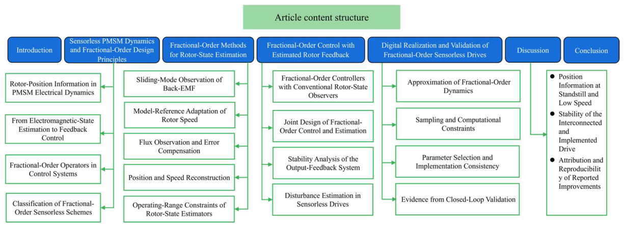
Figure 2.
PMSM electrical model and rotor-position information sources. (a) Stationary and rotating coordinate frames of the PMSM, with the rotor N-S axis and electrical rotor position. (b) Voltage/back EMF vector diagrams for surface-mount and interior PMSMs, illustrating the reluctance rotor asymmetry between the two machine topologies. (c) Reference-frame diagram of an IPMSM, showing the angular misalignment between the true d-q frame and the estimated frame used in MRAS position tracking. (d) Full order observer vector diagram in the synchronous rotating frame, showing the estimated flux, estimated position and position-error angle (Chen et al. 2003; Volpato Filho et al. 2021).
Figure 2.
PMSM electrical model and rotor-position information sources. (a) Stationary and rotating coordinate frames of the PMSM, with the rotor N-S axis and electrical rotor position. (b) Voltage/back EMF vector diagrams for surface-mount and interior PMSMs, illustrating the reluctance rotor asymmetry between the two machine topologies. (c) Reference-frame diagram of an IPMSM, showing the angular misalignment between the true d-q frame and the estimated frame used in MRAS position tracking. (d) Full order observer vector diagram in the synchronous rotating frame, showing the estimated flux, estimated position and position-error angle (Chen et al. 2003; Volpato Filho et al. 2021).
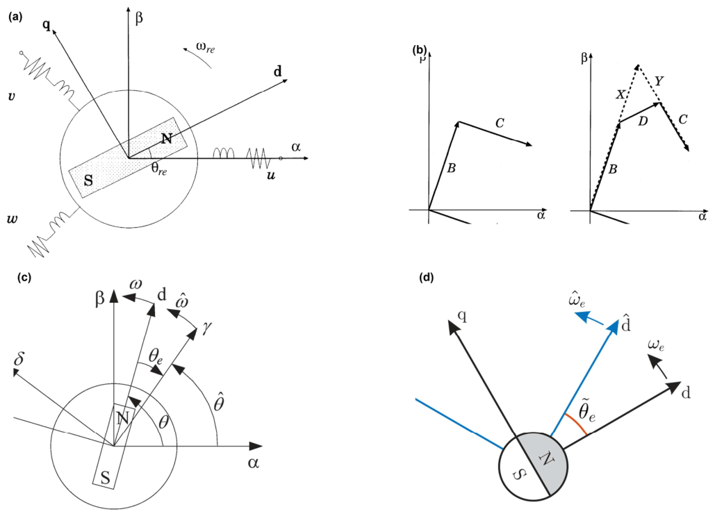
Figure 3.
Representative architectures of PMSM position sensorless drive systems. (a) Typical field-oriented vector control drive with an inner current loop, Park/anti-Park coordinate transformation, SVPWM inverter and a rotor position and speed observer. (b) General model based sensorless drive, showing the cascade from speed/position command, current regulation and inverter to the estimated back EMF and rotor position. (c) DSP based field-oriented control of a sensorless IPMSM drive over a wide speed range, integrating high frequency injection, dead time compensation and sliding mode estimation. (d) Main PMSM estimation branches, including open loop, disturbance-observer and full order observer structures, feeding a common position/speed estimation stage (Xu et al, 2023; Xu et al. 2018; Wang et al. 2012; Volpato Filho et al. 2021).
Figure 3.
Representative architectures of PMSM position sensorless drive systems. (a) Typical field-oriented vector control drive with an inner current loop, Park/anti-Park coordinate transformation, SVPWM inverter and a rotor position and speed observer. (b) General model based sensorless drive, showing the cascade from speed/position command, current regulation and inverter to the estimated back EMF and rotor position. (c) DSP based field-oriented control of a sensorless IPMSM drive over a wide speed range, integrating high frequency injection, dead time compensation and sliding mode estimation. (d) Main PMSM estimation branches, including open loop, disturbance-observer and full order observer structures, feeding a common position/speed estimation stage (Xu et al, 2023; Xu et al. 2018; Wang et al. 2012; Volpato Filho et al. 2021).
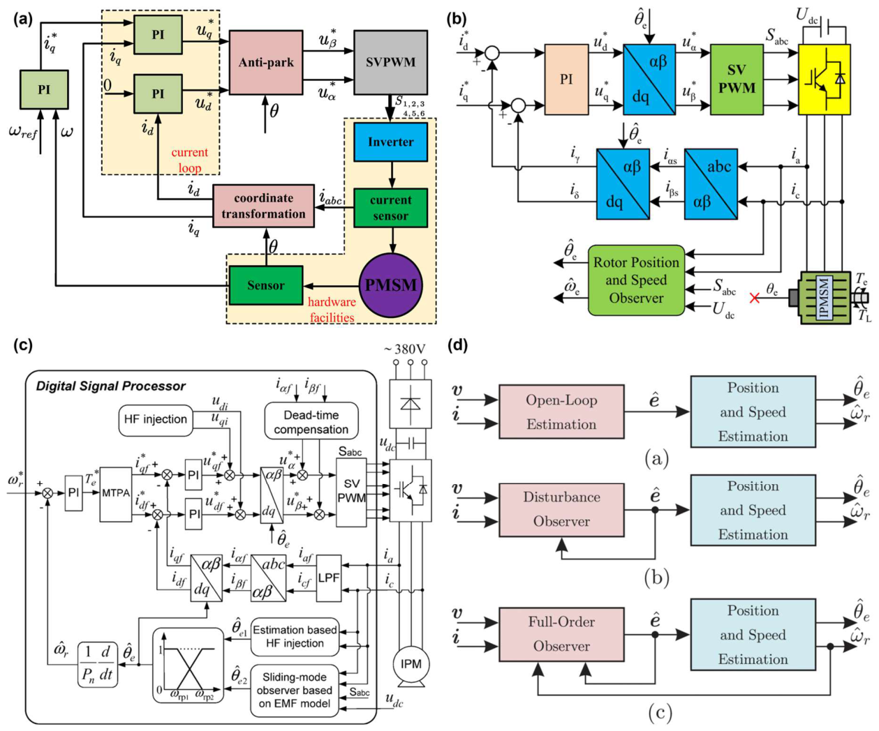
Figure 4.
Fractional order operators: definitions and frequency characteristics. (a) Geometric interpretation of the fractional order derivative as a power law memory kernel weighting the past trajectory. (b) Isodamping property of a fractional controller: flatness of the open loop phase response around the crossover frequency, yielding nearly constant phase margin over a broad frequency range. (c) Magnitude and phase Bode responses of Oustaloup recursive approximations of s^0.5 of different order compared with the ideal fractional operator. (d) Bode comparison between the true fractional operator s^0.18 and its integer order rational approximation, illustrating the valid approximation bandwidth (Ricardo et al, 2010; ALEKSEI et al, 2021; Furkan et al, 2020).
Figure 4.
Fractional order operators: definitions and frequency characteristics. (a) Geometric interpretation of the fractional order derivative as a power law memory kernel weighting the past trajectory. (b) Isodamping property of a fractional controller: flatness of the open loop phase response around the crossover frequency, yielding nearly constant phase margin over a broad frequency range. (c) Magnitude and phase Bode responses of Oustaloup recursive approximations of s^0.5 of different order compared with the ideal fractional operator. (d) Bode comparison between the true fractional operator s^0.18 and its integer order rational approximation, illustrating the valid approximation bandwidth (Ricardo et al, 2010; ALEKSEI et al, 2021; Furkan et al, 2020).
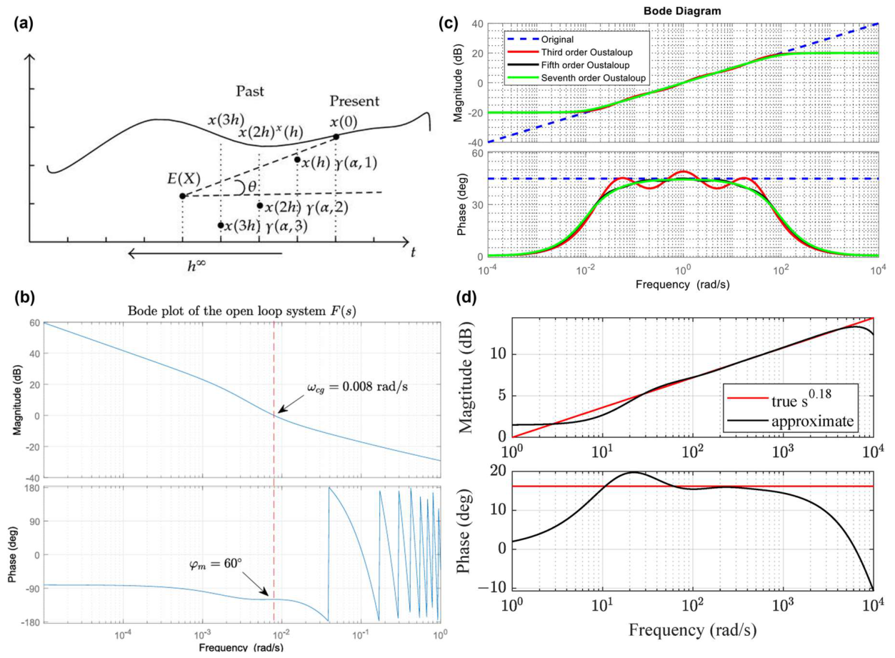
Figure 5.
Classification of fractional order sensorless PMSM schemes by the location of the fractional order operator. (a) Fractional order inside the observer: a nonlinear (terminal) extended state observer that extracts rotor position and speed from the extended back EMF through a nonlinear feedback (fal) function and cascade integrators. (b) Fractional order inside the model reference adaptation: fractional order model reference adaptive control with a model reference adaptive observer. (c) Fractional order adaptation law generating the estimated speed in a MRAS current error comparison loop. (d) Fractional order in both controller and observer: overall control diagram of a high-speed PMSM with LCL filter, combining a double closed loop vector control drive with a discrete fractional order terminal sliding mode observer (FNTSMO) and PLL in the sensorless branch. (e) Fractional order in the disturbance compensation branch: a repetitive fractional order active disturbance rejection speed controller cascading a repeating controller, delay compensation and a fractional order ADRC (Xu et al, 2020; Niu et al, 2022; Ahmed et al, 2021; Cheng et al, 2024; Zhao et al, 2026).
Figure 5.
Classification of fractional order sensorless PMSM schemes by the location of the fractional order operator. (a) Fractional order inside the observer: a nonlinear (terminal) extended state observer that extracts rotor position and speed from the extended back EMF through a nonlinear feedback (fal) function and cascade integrators. (b) Fractional order inside the model reference adaptation: fractional order model reference adaptive control with a model reference adaptive observer. (c) Fractional order adaptation law generating the estimated speed in a MRAS current error comparison loop. (d) Fractional order in both controller and observer: overall control diagram of a high-speed PMSM with LCL filter, combining a double closed loop vector control drive with a discrete fractional order terminal sliding mode observer (FNTSMO) and PLL in the sensorless branch. (e) Fractional order in the disturbance compensation branch: a repetitive fractional order active disturbance rejection speed controller cascading a repeating controller, delay compensation and a fractional order ADRC (Xu et al, 2020; Niu et al, 2022; Ahmed et al, 2021; Cheng et al, 2024; Zhao et al, 2026).
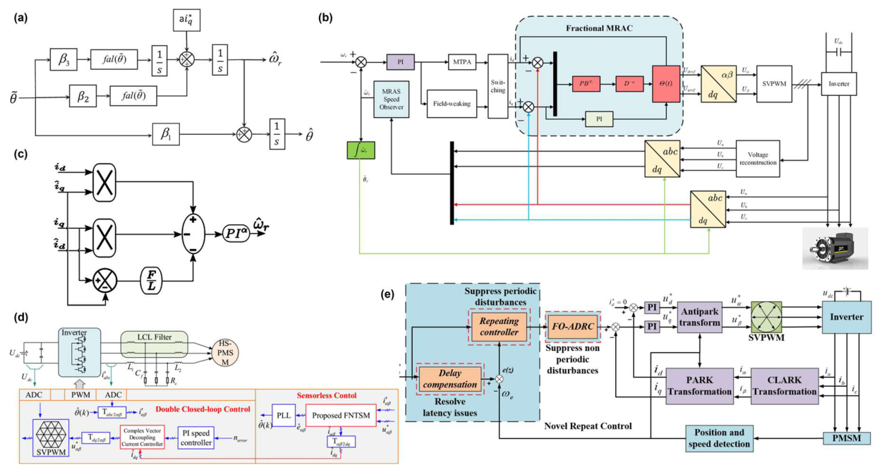
Figure 6.
Representative fractional order sliding mode observer (SMO) structures for back EMF estimation in PMSM position sensorless control. (a) Fractional order non-singular terminal SMO (FONTSMO) system control diagram, integrating fractional order sliding mode current control, adaptive feedback filtering and a fractional order phase locked loop. (b) Principle diagram of the nonsingular fast terminal SMO (NFTSMO) used to estimate the back EMF, showing the observer, terminal sliding mode surface, control law and back EMF calculation stages. (c) Sensorless control module embedding a fractional order super-twisting SMO (FO-STSMO) together with a double second order generalized integrator frequency locked loop cascaded with a control PLL (DSOGI-FLL-CPLL). (d) Algorithm flow of the full order terminal sliding mode observer (FOTSM observer) built on a fractional order model for smooth back EMF observation. (e) Double fractional order differential sliding mode surface combined with a super-twisting scheme and a complementary extended-state observer (Yao et al. 2024; Zhao et al. 2021; Huang et al. 2024; Zhou et al. 2025; Gao et al. 2025).
Figure 6.
Representative fractional order sliding mode observer (SMO) structures for back EMF estimation in PMSM position sensorless control. (a) Fractional order non-singular terminal SMO (FONTSMO) system control diagram, integrating fractional order sliding mode current control, adaptive feedback filtering and a fractional order phase locked loop. (b) Principle diagram of the nonsingular fast terminal SMO (NFTSMO) used to estimate the back EMF, showing the observer, terminal sliding mode surface, control law and back EMF calculation stages. (c) Sensorless control module embedding a fractional order super-twisting SMO (FO-STSMO) together with a double second order generalized integrator frequency locked loop cascaded with a control PLL (DSOGI-FLL-CPLL). (d) Algorithm flow of the full order terminal sliding mode observer (FOTSM observer) built on a fractional order model for smooth back EMF observation. (e) Double fractional order differential sliding mode surface combined with a super-twisting scheme and a complementary extended-state observer (Yao et al. 2024; Zhao et al. 2021; Huang et al. 2024; Zhou et al. 2025; Gao et al. 2025).
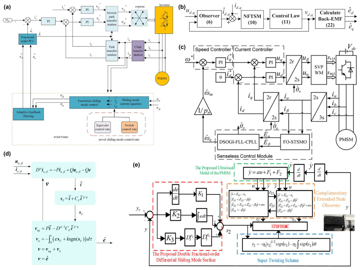
Figure 7.
Sampling and computational constraints. (a) PMSM experimental drive platform with an STM32H757 driver. (b) High-speed HSPMSM experimental platform. (c) Real-time direct-torque-control implementation bench. (d) PMSM experimental platform with a dsPIC digital signal controller (Wang et al, 2026; Cheng et al, 2024; Nicola et al, 2024; Xiao et al, 2022).
Figure 7.
Sampling and computational constraints. (a) PMSM experimental drive platform with an STM32H757 driver. (b) High-speed HSPMSM experimental platform. (c) Real-time direct-torque-control implementation bench. (d) PMSM experimental platform with a dsPIC digital signal controller (Wang et al, 2026; Cheng et al, 2024; Nicola et al, 2024; Xiao et al, 2022).
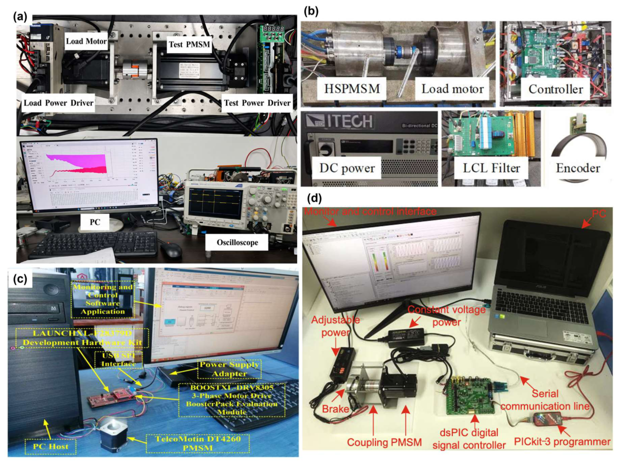
Table 2.
Structural and evidence-based comparison of core observation and position/speed estimation methods.
Table 2.
Structural and evidence-based comparison of core observation and position/speed estimation methods.
| Method class | Representative configuration | Fractional-order location | Estimated quantities | Measurements and model | Mathematical analysis | Applicability and evidence boundary | Sources |
|---|---|---|---|---|---|---|---|
| Fractional-order terminal sliding-mode observer | FONTSMO + adaptive back-EMF filter + FOPLL | Sliding surface and phase-locked loop | Back-EMF; rotor position; electrical angular speed | Stator voltage and current; SPMSM current model | Observer and filter Lyapunov arguments are presented but the reported gain condition and finite-time result are not sufficient as printed | SPMSM; implementation parameters of the fractional approximation are incomplete | [11] |
| Fractional-order sliding-mode observer | Fractional integral sliding surface + FO-PLL | Sliding surface and phase-locked loop | Back-EMF; rotor position; electrical angular speed | Stator voltage and current; PMSM current model | Ideal continuous-time reaching and PLL tracking arguments are presented; the realizable gain bound and complete fractional-order stability conditions are not established | The proof does not cover the Oustaloup states; nonzero initial conditions; boundary layer; or digital implementation | [12] |
| Fractional-model terminal sliding-mode observer | μ-order current model + full-order terminal SMO + GQPLL | Fractional-order plant/observer model | Back-EMF; rotor position; electrical angular speed | Stator voltage and current; assumed μ-order PMSM model | Terminal sliding-mode analysis is presented but the printed model and error equations contain unresolved dimensional and sign issues | The fractional order μ and model-identification evidence are not reported | [29] |
| Active-flux super-twisting sliding-mode observer | Active-flux model + STW-SMO + back-EMF observer + FO-SPLL | Phase-locked loop | Active flux/back-EMF; rotor position; electrical angular speed | Stator voltage and current; effective-flux model | Lyapunov and super-twisting arguments are presented; consistency of the printed two-axis equations and convergence after tanh replacement require caution | Applicable when the effective-flux magnitude is approximately constant; the boundary-layer implementation supports practical rather than exact convergence | [23] |
| Integer-order sliding-mode observer with fractional-order PLL | SMO or NFTSMO + FO-(S)PLL | Phase-locked loop only | Back-EMF; rotor position; electrical angular speed | Stator voltage and current; αβ or dq PMSM model | Observer reaching and PLL analyses are separated; reported conditions do not establish stability of the implemented output-feedback loop | The observer itself is integer order; low-pass compensation and dq-frame angle-error coupling must be checked for each implementation | [13,22] |
| Active-flux variable-gain sliding-mode observer | Active-flux VGSMO + FO-PLL | Phase-locked loop only | Active flux; rotor position; electrical angular speed | Stator voltage and current; active-flux model for SPMSM/IPMSM | A Lyapunov-type observer argument is given but the derivation assumes the estimated angle equals the actual angle and the printed error dynamics are inconsistent | Potentially covers SPMSM and IPMSM through active flux; the proof does not establish the actual angle-coupled closed loop | [32] |
| Voltage-model flux observer with fractional-order PLL | Leakage integrator/high-pass flux observer + FO-PLL | Phase-locked loop only | Permanent-magnet flux; rotor position; electrical angular speed | Stator voltage and current; SPMSM voltage model | PLL transfer-function tuning is reported; no complete output-feedback stability proof is provided | Leakage integration mitigates drift but introduces magnitude/phase error; the cutoff frequency and complete realization are incompletely reported | [14] |
| Model-reference adaptive observer/system | MRAO with PI speed adaptation; or current-model MRAS with fractional second-order sliding adaptation | Speed-adaptation law or associated fractional-order controller depending on the study | Electrical angular speed; current/state variables | Measured currents; reference and adjustable PMSM models | Popov/Lyapunov-type analyses are reported but the printed error signs; semidefinite conclusions; initial manifold and fractional realization must be verified case by case | Fractional order is not located in the same subsystem across these studies; reproducibility depends on complete operator and approximation reporting | [15,16] |
| Conformable fractional-order extended-EMF observer | Conformable FO-EEMF observer | Extended-EMF observer dynamics | Extended EMF; rotor position/speed for comparison | Stator voltage and current; IPMSM extended-EMF model | The conformable derivative reduces to a time-varying local derivative under the stated limit; the printed observer and Lyapunov equations contain unresolved injection and cross-term issues | Experiments use encoder speed feedback and do not demonstrate sensorless closed-loop operation | [19] |
| Flux observer with fractional-order resonant error compensator | Flux observer + FOQR-ESO position-error compensation | Fractional quasi-resonant extended-state error-correction channel | Position-error harmonic component; corrected rotor position | Measured currents and commanded/applied voltages; flux-observer position | Component-level stability arguments are provided; stability of the combined characteristic expression and complete output-feedback loop is not established | FOQR-ESO is a position-error compensator rather than the primary position observer; tested minimum speed is 300 r/min and does not establish zero-speed operation | [4] |
Table 3.
Controller–observer configurations and the scope of their mathematical analysis.
| Controller | Observer or estimator | Fractional-order location | Feedback variable | Analysis object | Reported evidence | Evidence boundary | Sources |
|---|---|---|---|---|---|---|---|
| FOPI speed and current loops | MRAS/MRAO | Controllers and adaptation block depending on study | Estimated speed and integrated position | Controller/MRAS components | Selected speed/load profiles | Incomplete full estimation-error and output-feedback proof | [27,50] |
| FO controller variants in DTC | Integer-order flux observer | Controller only | Estimated flux angle/speed or torque | Mostly controller/observer components | Selected simulation/HIL responses | Observer accuracy and causal FO contribution not isolated | [17] |
| FOPI/FOPID speed loop | Smooth super-twisting observer plus PLL | Controller only | Estimated position and speed | Reduced observer/controller components | Selected positive-speed profiles | Multiple blocks changed and key parameters missing | [52] |
| FO sliding-mode outer loop | Integer-order EKF | Controller only | EKF speed and position | Controller and EKF components | Selected simulated profiles | Sampling/covariance/observability/full-loop proof missing | [51] |
| FO integral sliding-mode controller | Integer-order ASMO plus EHGO | Controller only | Cascaded position/speed/disturbance estimates | Controller and observer separately | Simulation and specified load-switch test | Implemented feedback law differs from parts of proof; no full-loop theorem | [18] |
| Fractional speed controller | Integer-order current-model MRAS | Controller only | Estimated speed and integrated position | Sliding variable/MRAS components | Selected simulation and hardware speeds | No matched baseline or quantified hardware estimation error | [25] |
| 0.8-order integral sliding controller | Fractional-order SMO | Controller and observer correction | Estimated back-EMF position and speed | Ideal controller and integer comparison observer proofs | Selected simulated speed conditions | Actual FO observer and full output-feedback loop not proven | [28] |
| Conventional PMSM controller | Flux observer plus FOQR-ESO compensator | Fractional quasi-resonant error-correction channel | Corrected position | Component/common characteristic analyses | Hardware at 300/600/2000 r/min | Compensator is not primary observer; time-varying/full-loop proof incomplete | [4] |
Table 4.
Discrete realization and parameter-tuning record for fractional-order controllers and observers.
Table 4.
Discrete realization and parameter-tuning record for fractional-order controllers and observers.
| Sources | Operator location | Operator definition | Realization | Band or memory | Sampling and platform | Reported cost | Tuning method | Reproducibility boundary |
|---|---|---|---|---|---|---|---|---|
| [11] | Sliding observer/filter/PLL | RL-related notation with inconsistencies | Oustaloup stated | NR | NR | NR | Controller/observer parameters reported incompletely | Definition sign and approximation parameters incomplete |
| [27] | FOPI controllers | RL integral | Product trapezoidal history convolution | Step/history NR | NR | NR | PSO joint tuning | PSO settings final parameters and memory implementation incomplete |
| [26] | Fractional nonlinear observer term | RL-related derivative with reset | Sign-event timing reset plus discrete realization | Hybrid memory/reset details incomplete | NR | NR | Design parameters in paper | Reset implementation not automatically equivalent to fixed-terminal history operator |
| [12] | Sliding surface and PLL | Fractional integral/transfer representation | Oustaloup stated | Order/band incomplete | NR | NR | Gain/PLL design | Continuous proof excludes approximation boundary layer and sampling |
| [13,14] | PLL/filter | Fractional loop-filter transfer function | Rational approximation stated or implied | Key cutoff/band items NR | NR | NR | Frequency-domain parameters | Observer remains integer order and realization reporting is incomplete |
| [50] | Four FOPI loops | RL integral | Product trapezoidal history convolution | Step/history NR | NR | NR | PSO; orders 1.0564/1.4691/1.1891/1.13 | Search settings histories and closed-loop FO stability incomplete |
| [18] | FO integral sliding controller | RL fractional integral and sign-related derivative | NR | NR | Sampling/platform load NR | NR | VGWO 30 agents 150 iterations 17 parameters | Several boundary results and no repeated-run statistics or digital realization |
| [28] | FO controller and FOSMO | Fractional integrals in controller/observer | NR | NR | Hardware not reported for proposed validation | NR | Stochastic optimization | Single seed and key population/repetition/model parameters incomplete |
| [4] | FO quasi-resonant ESO correction | Fractional quasi-resonant state realization | Finite-dimensional 13-equation implementation | Targeted sixth-order periodic error | STM32H757 at 16 kHz | 9.85 μs component time; ESO 3.79 and IOQR 5.43 μs | Structured parameter design | Does not equal full-loop WCET and is not portable across platforms |
Table 5.
Performance evidence organized by metric, operating condition, baseline, ground truth, and applicability boundary.
Table 5.
Performance evidence organized by metric, operating condition, baseline, ground truth, and applicability boundary.
| Sources | Metric | Operating condition | Baseline | Ground truth or feedback | Reported result | Implementation or cost | Applicability boundary |
|---|---|---|---|---|---|---|---|
| [11] | Speed/position error and current THD | 800→1000 rad/s; 8 N·m; additional 1000→1200→1000 rad/s and load tests | Conventional and second-order SMO | Feedback role incompletely reported | Load-stage speed error 4.60/4.10/1.760 rad/s; position error 0.050/0.042/0.018 rad; THD 17.81/7.86/5.36% | Approximation parameters incomplete | Combined observer/filter/PLL effect under reported tests |
| [26] | Position error and transient angle disturbance | 20–60 kr/min; I–F start; 4.5 N·m at 60 kr/min | Tustin/RK and Luenberger comparisons | Encoder/bench reference per source | Selected position errors and smaller transient disturbances; Luenberger can have slightly better steady accuracy | Discrete/reset details require caution | High-speed machine-specific evidence; not low-speed/full-range proof |
| [12] | Maximum position error and signal ripple | 1500/3000 r/min; observer feedback only above 600 r/min | Conventional SMO | Encoder angle used in comparison | Approx. 20° versus 12° maximum position error at rated condition | Oustaloup/sampling details incomplete | Requires prepositioning and I–F start; no zero-speed evidence |
| [19] | Observer output comparison | Reported hardware conditions | Conventional observer variants | Encoder speed remains in control feedback | Observer-component results only | Implementation details examined | Not a sensorless closed-loop validation |
| [15] | Speed/angle error and load recovery | 0→1500→−1500 r/min; 100 r/min; ±1 N·m | Author baselines | Model/encoder reference per source | Reported speed/angle error reductions and approx. 0.03 s recovery with potentially large peak | Implementation and physical-order comparability incomplete | Nonzero selected speeds; no full-range/physical identification proof |
| [50] | Tracking waveforms and transient undershoot | 1000→2000; 10→50→100 r/min no-load; +10→−10; 2000→100 r/min | No matched integer/ablation baseline | Model truth | Tracking shown; separate deceleration has about −100 r/min undershoot | PSO and history realization incomplete | 10 r/min is ideal no-load model test; no zero-speed/hardware proof |
| [18] | Speed standard deviation and maximum absolute deviation | 1000 r/min; 0.16/0.32 N·m load switching | PID and ISMC | No quantified encoder-based state-estimation error | Std. dev. 17.12/9.95/6.43 r/min; FOISMC vs ISMC max-absolute-error improvement only 0.49 r/min | Discrete FO/processor/optimizer repeats NR | Controller and observer effects not isolated |
| [28] | Angular error | 1000 r/min selected condition | Controller/observer configurations | Model truth | Maximum approx. 0.067 rad; RMSE approx. 0.029 rad | Hardware and key reproduction data absent | Does not establish zero/low/full-speed performance |
| [4] | Position-error IAE spectral components transient error and component time | 300/600/2000 r/min; load and speed transients | ESO and IOQR-ESO | Encoder used only for evaluation | FOQR IAE reduction 69.83/54.24/53.02%; IOQR 57.08/32.74/36.94%; mixed transient/frequency results | STM32H757 16 kHz; 3.79/5.43/9.85 μs component times | Lowest speed 300 r/min=15% rated; no zero-speed proof; component timing only |
Disclaimer/Publisher’s Note: The statements, opinions and data contained in all publications are solely those of the individual author(s) and contributor(s) and not of MDPI and/or the editor(s). MDPI and/or the editor(s) disclaim responsibility for any injury to people or property resulting from any ideas, methods, instructions or products referred to in the content. |
© 2026 by the authors. Licensee MDPI, Basel, Switzerland. This article is an open access article distributed under the terms and conditions of the Creative Commons Attribution (CC BY) license (http://creativecommons.org/licenses/by/4.0/).
Copyright: This open access article is published under a Creative Commons CC BY 4.0 license, which permit the free download, distribution, and reuse, provided that the author and preprint are cited in any reuse.