

Submitted:
30 September 2026
Posted:
01 October 2026
You are already at the latest version
Abstract
The article investigates different scenarios of self-production decentralized photovoltaics, aiming at the maximization of the power demand real-time coverage of five different types of final consumers: typical residences, a typical commercial facility (travel agency), an industrial facility, the Hellenic Mediterranean University main campus and the Crete Aquarium (exhibition facility). The different types of final users impose different daily power demand profiles, which highly affects the potential for real-time concurrent power production from the photovoltaics. All these facilities are located in the insular Greece, with high incident solar radiation and mild ambient temperatures during winter and summer, favoring the maximization of the panels’ efficiency. The photovoltaic plants operate only as self-production plants, without any commercial activity, namely the produced electricity is only used for real-time power demand compensation or storage, without ever being sold in the electricity market. The article is based on the investigation of alternative scenarios regarding the sizing of the photovoltaic plants and their potential support of decentralized electrochemical batteries. The process is based on the computational simulation of the plants, based on annual power demand and production time series of average hourly values. The results show high potential for real-time power demand coverage for the commercial and the exhibition facility (higher than 45% of the annual electricity consumption), thanks to the considerable power consumption during daytime, while this potential remains rather poor for residential buildings (25-28%). The payback periods may be at the range of 4-6 years. The introduction of batteries can increase considerably the annual electricity consumption compensation, reaching percentages higher than 90%, yet with deterioration of the economic feasibility of the investment (payback periods higher than 8 years).
Keywords:
self-production photovoltaics
; decentralized electricity production
; electrochemical storage batteries
1. Introduction
Due to the considerable increase in socioeconomic development, electricity demand has witnessed continuous growth [1]. Traditional fossil fuels have had a damaging effect on the environment over the years [2], with greenhouse gas emissions contributing to global warming and climate change [3]. The global shift towards cleaner energy sources constitutes a vital aspect of reducing dependence on fossil fuels and ensuring energy security [4]. Among various options of Renewable Energy Sources (RES), solar [5,6] and wind power [7,8,9] stand out as the most technologically mature and widely deployed choices [10], providing abundant and clean generation. However, their intermittent variability poses significant challenges to electrical grids [11] introducing uncertainty into generation planning [12].
Energy storage systems (ESS) can offer a promising solution to this variability [13] by absorbing the renewable energy surplus during periods of low demand and injecting it back to the grid when the RES output is low [14]. Common forms of energy storage technologies can be divided into three categories [15]: mechanical storage, including Pumped Hydro Storage (PHS) [16] and Compressed Air Energy Storage (CAES) [17], electrochemical storage, most notably lithium-ion batteries [18] and chemical fuel storage, such as hydrogen [19,20]. Abdon et al. [21] proposed an assessment methodology for comparing stationary electricity storage technologies, considering their overall performance in technical, economic and environmental terms. The study showed that for short time scales, battery energy storage stands out as the most advantageous solution, while for larger-scale systems, PHS and CAES show the best performance. Small PHS and micro-CAES systems can be also foreseen even in small, non-interconnected applications, if high RES secure penetration constitutes a main objective [22,23].
The decentralized nature of RES-ESS deployments is reshaping electrical systems into a decentralized model [24], moving the generation physically closer to the consumption [25]. This approach results in reduced transmission and distribution losses while also strengthening the security of energy supply [26]. It has also led to the emergence of consumers evolving into the so-called ‘prosumers’ [27], consumers who actively manage their energy requests using generation and storage systems [28,29]. Building on this shift, energy communities, defined as a group of consumers, producers and prosumers collaborating to optimize energy production, consumption and distribution [30], are gaining prominence as a mechanism to accelerate the involvement of citizens in the energy transition [31], representing a viable path towards a cleaner and more democratized energy future [32,33]. Santos et al. [34] proposed a community energy management system to evaluate a price-based demand response strategy within the Brazilian Time-of-Use tariff system framework, utilizing distributed, shared photovoltaic (PV) systems and Battery Energy Storage Systems (BESS) among community members, with results demonstrating daily financial savings of around 20%.
One of the most advantageous characteristics of PV systems is their modularity: they remain economically and technically viable across different scales, from residential installations to utility-sized plants [35]. Two electricity pricing schemes that dominate the PV electricity market are net metering and net billing [36]. In both cases, the energy surplus is exported to the grid, but they differ in how this surplus is valued. Under net metering, excess electricity is credited against future consumption at the retail electricity price, while in the net billing case, it is credited at a lower rate [37]. In recent years, a transition from net metering to net billing is being observed in many countries [38], including Greece. In the Greek context, net metering has been proven more advantageous, offering faster and stable investment returns and protection against price fluctuations [39]. Simoglou et al. [40] assessed the application of net-metering and net-billing PV self-consumption schemes for residential and industrial consumers in the Greek context, reporting annual average self-consumption rates of 45–50% for residential consumers and 51–69% for industrial consumers. This study further confirmed the comparative advantage of net metering in comparison to net billing.
To overcome the difficulties arising from standalone PV systems under the net billing scheme, the integration of a BESS offers a practical solution. BESS mitigates PV intermittency [41], increases self-consumption and reduces energy imported from the grid [42]. Their scalability and easier installation, in comparison with PHS and CAES [43], can provide the required flexibility to match the energy demand and store the surplus generation [44]. Combined with their steadily decreasing costs [45] and their fast response [46], these characteristics have positioned BESS as a central technology in the ongoing energy transition. An et al. [47] optimized the dimensioning of BESS in urban areas with the objective of maximizing the self-sufficiency rate, minimizing peak load and maximizing the economic benefit. The results indicated that small-scale BESS installations in buildings were effective in maximizing self-consumption, however, the associated economic benefits remain limited.
Chen et al. [48] proposed a multi-objective optimization approach for PV-BESS systems within building energy sharing communities, comprising factories, offices and dormitories. The optimization objectives were to maximize the PV self-consumption rate, minimize the payback period and reduce power transportation loss. PV power generation and the power demand of each building were identified as the most influential parameters regarding BESS allocation priority, while overall system BESS capacity was governed by PV array surface area, peak-to-valley price differences and grid-imposed limits on energy imports and exports.
Lara et al. [49] evaluated the economic feasibility of BESS integrated with PV for self-consumption purposes in the Dominican Republic’s residential sector. Results showed that BESS integration increased the self-consumption rate from 73.4% to 98.3%, while reducing overall profitability due to higher investment costs. The analysis further showed that PV self-consumption was profitable only for high-demand users, with profitability being strongly correlated with the hourly demand profile.
Migliari et al. [50] assessed the cost-effectiveness of PV-BESS for self-supply across various European electricity markets, with the market of Sardinia demonstrating strong economic viability. Conversely, the markets of Spain and Germany exhibited weaker profitability, attributable to the frequent occurrence of low or negative electricity prices, with several configurations yielding negative returns. Although BESS integration increased self-consumption, it did not enhance the economic viability of the projects, with lower nominal-capacity systems proving more feasible.
2. Scope and Novelty of the Article
The present article focuses on the investigation of the energy and economic feasibility of the introduction of decentralized photovoltaic plants, with or without the support of electrochemical batteries, aiming at the maximization of the power demand real-time coverage in five different types of consumers:
- university;
- exhibition facility;
- industrial facility;
- residential buildings;
- commercial facility.
The investigated facilities are located in Crete, hence, the outcomes of this work refer to the Mediterranean basin, regarding both the climate conditions and the power demand daily profiles.
The article anticipates to emphasize on the potential for power demand real-time coverage from decentralized photovoltaic plants operating under the net-billing, self-production mode, with or without storage support, concluding in definite results regarding the annual electricity coverage percentage and the economic anticipated savings. By examining different types of consumers, the effect of the power demand daily profile on the real-time demand coverage is examined and the results of the study are classified respectively.
3. Methodology and Data
The methodology adopted in this article is based on the computational simulation of the annual power demand and production from photovoltaic panels for each one of the under consideration consumers. For the cases of the academic institute, the exhibition facility and the industrial consumer, real annual power demand time series of average hourly values were employed for:
- the main campus of the Hellenic Mediterranean University (HMU);
- the Crete Aquarium;
- an aluminum frames manufacturing factory.
These power demand time series were officially supplied by the electricity provider of these facilities. All the above facilities are located at the northern coastline of Crete (Prefecture of Heraklion).
For the case of the commercial facility, real power demand daily profiles were employed from a travel agency for particular periods during the year, located also in Heraklion, Crete. The annual power demand time series was arithmetically developed.
Regarding the residential buildings, power demand daily profiles were retrieved from the scientific literature, referring also to the case of a typical Greek city. All these power demand data are presented in detail in the following Section 3.1.
The meteorological data required for the calculation of the power production from the photovoltaics, such as the incident solar irradiance on horizontal plane and the ambient temperature, were downloaded for the under consideration geographical area (the city of Heraklion, Crete) from the European Centre for Medium-Range Weather Forecasts (ECMWF) [51]. Wind velocity data were retrieved from certified measurements provided by the Hellenic Mediterranean University. They are in detail presented in the following Section 3.2.
Finally, the main operation simulation algorithm is explained in Section 3.3.
3.1. Power Demand Data
3.1.1. HMU, Crete Aquarium and Industrial Facility
The annual power demand fluctuation for the main campus of the Hellenic Mediterranean University and the Crete Aquarium are presented in Figure 1 and Figure 2 respectively.
The impact of the holiday seasons in Christmas, in Easter and on August is clearly depicted in Figure 1 for the power demand of the academic institute. This impact is totally absent in the case of the Aquarium. On the contrary, in the case of the Aquarium the power demand is maximized in summer, particularly due to the increasing attendance during the tourist season.
For a more detailed picture on the daily power demand fluctuation, daily power demand curves are given for the two facilities in Figure 3 and Figure 4, for specific periods during the year. In Figure 3, the daily power demand fluctuation is given for the period from the 11th to the 20th of February in HMU, while in Figure 4 the daily power demand fluctuation is given for the period from the 25th of July to the 4th of August in Crete Aquarium. In both graphs it is seen that the power demand increases during daytime, a feature highly favorable regarding the potential for real-time power demand coverage from the photovoltaics production. The impact of the weekend on the power demand is also clear in the case of HMU (Figure 3), while it is totally absent in the case of the Crete Aquarium.
Similarly, for the aluminum frames manufacturing factory, the annual power demand time series is presented in Figure 5, while in Figure 6, the power demand fluctuation is depicted for a particular ten-day period. The factory remains inoperative for a ten-day period in August and on Sundays, as clearly depicted in these figures.
Finally, as in the case of HMU and the Crete Aquarium, power demand in this factory also maximizes during daytime, a feature highly favorable regarding the maximization of the real-time power demand coverage directly from the photovoltaic power production.
3.1.2. Residential Buildings
Regarding the power demand in residential buildings, typical daily power demand profiles were retrieved from the scientific literature, which are presented in Figure 7 and Figure 8 [52]. It is worth noting that these curves are based on actual measurements, coming from a sample of 120 residences from the city of Thessaloniki, Greece. For this reason, they were preferred over corresponding available curves based on theoretical models.
As seen in Figure 7 and Figure 8, the shape of the daily residential electricity demand profiles reveals that demand peaks during the morning hours—roughly between 7:00 and 9:00—and the evening hours—approximately between 17:00 and 19:00—whereas, conversely, power demand remains low during the peak production hours of photovoltaics (i.e., around midday). This situation clearly does not favor maximizing the balancing of electricity consumption against production.
The development of the annual power demand time series for the residential users was based on the daily residential demand profiles presented in Figure 7 and Figure 8. The following percentage contributions of the profiles shown in these figures are assumed for the composition of the total power demand:
- profiles 1–4: 10% each (40% in total)
- family with 1 child: 20%
- family with 2 children: 30%
- family with 3 children: 10%.
Based on the aforementioned percentage contribution of each daily profile, a composite power demand daily profile for a number of residences is ultimately established. The annual power demand time series is developed arithmetically by replicating this daily curve for every day of the year and applying monthly weighting factors per day (from 0.923 to 1.091), in order to account for the impact of seasonality and climatic conditions on the magnitude of residential power demand, while securing a smooth power demand fluctuation from day to day and from month to month over the year. The final, annual power demand curve for a mixture of 100 residences is presented in Figure 9, while in Figure 10 the power demand fluctuation is given for a period of 10 days.
3.1.3. Commercial Facility
The case of the commercial facility is approached with a travel agency, located in Heraklion, Crete. For this specific facility, real power demand daily profiles were available for limited and indicative time periods during the year (e.g., one week in June, another one in August, one week in December etc). Given the available power demand data, the annual power demand time series was developed arithmetically, taking into account that the main power demand in the specific facility is formulated by the indoor space conditioning load and the computational infrastructure (PCs, server etc). The annual power demand fluctuation for the travel agency is given in Figure 11, while in Figure 12 a focused power demand fluctuation graph is given for a ten-day period during the peak demand season (August).
In these figures it is seen that, sensibly, the power demand in the travel agency is maximized in summer, due to the increasing indoor space cooling needs, as well as the increasing work load during the tourist season. It is also seen that the power demand is maximized during daytime, which favors the maximization of the real-time power demand coverage from the photovoltaic power production. However, it is also seen that there is a constant base load, always present, even during nighttime, obviously due to the constant operation of the computational infrastructure (the central server of the facility). This fact limits the maximum possible concurrent power consumption coverage from the photovoltaics and induces the introduction of storage support.
3.1.4. Power Demand Section Synopsis
In the overall section 3.1 annual power demand time series, all of them based on real measurements and available data, were presented for all the investigated facilities:
- the main campus of the Hellenic Mediterranean University;
- the Crete Aquarium;
- an aluminum frames manufacturing factory;
- a travel agency;
- a mixture of 100 residences.
The essential power and electricity consumption data from these facilities are summarized in Table 1.
For the HMU and the Crete Aquarium, as seen in Table 1, apart from the electricity consumption, electricity procurement cost data were also available. The electricity procurement specific cost is calculated as the ratio of the total annual procurement cost over the electricity consumption. Given that for the rest investigated consumers there were no cost data available, the calculated electricity procurement specific cost for the HMU and the Crete Aquarium will be also used for the rest investigated facilities for the economic evaluation of the examined photovoltaic plants.
It should be also stated that all the under consideration facilities, apart from the residential buildings, exhibit peak power demand during daytime, a feature highly favorable towards the maximization of the real-time power demand coverage from the photovoltaic power production.
3.2. Meteorological Data and Photovoltaic Production
3.2.1. Meteorological Data
Apart from the wind velocity, the rest meteorological data required for the calculation of the photovoltaic power production were downloaded from the European Centre for Medium-Range Weather Forecasts (ECMWF) [51] for the geographical point with coordinates 35.25ο N – 25.25ο E, located approximately 8.5 km south from the northern coastline of Crete. Specifically, annual time series of average hourly values for the year 2025 were downloaded for the ambient temperature and the clear sky incident solar irradiance on horizontal plane, presented in Figure 13 and Figure 14 respectively.
Annual wind velocity certified measurements were retrieved from the Energy Systems Laboratory of the Mechanical Engineering Department of the Hellenic Mediterranean University. The measurements were captured in 2013 at the wind speed certified field (35.31o N, 25.10o E) of the specific Laboratory. Although they are not concurrent with the rest meteorological data, which refer to 2025, they were selected as the most reliable and accurate available wind measurements, compared to the ECMWF data. The annual wind velocity fluctuation is presented in Figure 15.
The hourly average ambient temperature ranges from 5.2 oC to 33.1 oC, exhibiting an annual average of 18.7 oC. The annual average wind velocity is calculated at 5.0 m/s, with prevailing wind blowing direction from northwest. The relatively low temperature and the northwestern blowing winds favor the efficient operation of the photovoltaic panels, by maintaining the photovoltaics’ cells temperature as close to the standard test operation conditions as possible (25 oC) [53].
Finally, as seem in Figure 14, the daily maximum clear sky incident solar irradiance on the horizontal plane ranges from the 300 – 400 W/m2 in winter to 854 W/m2 (maximum annual value) in summer, while the annual, cumulative solar irradiation is calculated at 1667.2 kWh/m2, revealing the high available solar potential in the under consideration geographical area.
Following the essential principles and relationships of solar geometry and radiation [54], the annually incident cumulative incident solar irradiation on inclined south-facing surface was calculated versus different tilts with regard to the horizontal plane. Table 2 summarizes the results of this calculation, highlighting that the optimum installation angle of photovoltaic panels at the northern coastline of Crete is 30o.
For the optimum installation tilt for the photovoltaic panels, Figure 16 presents the annual fluctuation of the incident solar irradiance on a south-facing flat surface, broken down into its components: direct, diffused and reflected. The total incident solar irradiance, derived from the sum of these components, is used for the calculation of the photovoltaic power production.
3.2.2. Photovoltaic Power Production
The photovoltaic power production calculation process is based on an essential, empirical methodology described in the relevant literature [55]. In a comprehensive approach, the photovoltaic power production Ppv is given by the following relationship:
where cpv the photovoltaic panel power factor and Pnom the nominal, installed photovoltaic power.
The photovoltaic power factor cpv is given by the relationship:
where:
- PRopt, PRNIT and PRT are, respectively, the optical performance ratio (related to shading or soiling losses), the non-irradiance and temperature performance ratio (expresses losses in the inverter, not related to solar irradiance or cell’s temperature) and the temperature performance ratio (expresses losses related to the cell’s temperature)
- ηtrans the electricity transportation losses in the cabling and the transformer.
In this work, typical values for PRopt, PRNIT and ηtrans equal to 97.5%, 97.0% and 98.5% are respectively adopted.
The temperature performance ratio PRT is given by the following relationship:
where:
- is the cell’s temperature at Standard Test Conditions, equal to 25 oC;
- γmp is the temperature coefficient of maximum power: it represents the photovoltaic power production drop percentage for every oC (or K) of the cell’s temperature above the , adopted equal to -0,0045 K-1;
-
is the weighted average cell temperature: the real temperature of the photovoltaic cell.The photovoltaic cells’ real temperature is given by the following relationship:
- is the ambient temperature (Figure 13);
- F is the mounting/installation factor: it represents how well the system is ventilated (e.g., whether it is ground-mounted or roof-integrated);
- is the wind cooling coefficient, where wSD is the wind speed (Figure 15): it expresses the reduction in panel temperature due to the cooling provided by the wind;
- G is the incident solar irradiance on the photovoltaic panels’ surface (Figure 16).
Τhe mounting/installation factor F is given by the following relationship:.
and, finally, the wind cooling coefficient is given by the following relationship:
- T1 is the initial temperature rise component, equal to 19.6 ∘C: this parameter represents the maximum thermal contribution to the cell’s temperature rise above ambient conditions under stagnant air (zero wind speed), normalized per unit of standard irradiance;
- B is the exponential wind cooling constant, equal to −0.223 (m/s)-1: this is an empirical exponential decay factor that quantifies the convective cooling effect of the wind. The negative sign ensures that as wind speed wSD increases, the exponential term decreases, accurately modeling the heat dissipation from the module’s surfaces;
- T2 is the constant thermal offset, equal to 11.5 ∘C: it is a constant temperature parameter that represents the baseline thermal equilibrium shift of the photovoltaic module under steady-state operational conditions;
- Δθ is the internal thermal gradient, equal to 3 ∘C: this parameter accounts for the internal temperature difference between the core photovoltaic silicon cell Tcell and the module’s front glass surface Tmodule, caused by the conductive thermal resistance of the encapsulation layers;
- GSTC is the reference solar irradiance, equal to 1000 W/m2.
By applying the above presented methodology with the adopted values for the involved parameters and the meteorological data presented in section 3.2.1, the annual power production time series per kWp of installed photovoltaic power is calculated. It is presented in Figure 17. The annual final produced electricity per kWp of installed photovoltaic capacity is calculated by integrating this time series at 1587.7 kWh, corresponding to an annual, final capacity factor of 18.1%.
3.3. Computational Simulation Approach and General Data and Parameters
The computational simulation algorithm is simple and, practically, considers each one of the investigated final users as an autonomous consumer, aiming to maximize the photovoltaic real-time penetration in the power demand coverage, with or without the support of electrochemical batteries. Specifically, for each hourly calculation time step t, the following steps are applied:
- If Pd is the current power demand and Ppv is the current photovoltaic power production, then the real-time power demand coverage Pd-pv from the photovoltaic power production is calculated from the following relationship:
- 2.
- The remaining power demand Pd-rem not directly covered by the concurrent photovoltaic production is:
- 3.
- The photovoltaic power Ppv-st which is potentially available for storage is:
- 4.
- If Cbat is the batteries’ storage capacity, ηst the storage efficiency and Est(j-1) the batteries’ charge level from the previous time step, then the absorbed photovoltaic power for storage Pst is:
- 5.
- If ηdis is the batteries’ discharge efficiency and Emin the batteries’ minimum possible charge level, then the power demand coverage from the batteries Pbat is:
- 6.
- The batteries’ new charge level Est(j), at the end of the current time step is:
The above presented computational calculation process is applied iteratively for all the investigated final users and for different scenarios regarding the sizing of the photovoltaic plant and the storage capacity of the potential electrochemical batteries.
The final evaluation of each scenario under consideration is completed based on the calculation of the following key metrics:
- percentage of annual electricity demand coverage from the combined output of the photovoltaic plant and the battery storage system, calculated versus the annual electricity demand;
- percentage of annual electricity production surplus from the photovoltaic plant (production that is neither concurrent with power demand nor storable), calculated versus the plant’s initial annual electricity production;
- reduction in annual electricity procurement costs, calculated as the product of the annual electricity demand coverage and the existing procurement specific cost (0.2524 €/kWh for HMU and 0.2172 €/kWh for all the rest users);
- payback period, calculated as the ratio of the initial investment cost to the annual reduction in electricity procurement costs;
- specific cost of annual electricity coverage, calculated using the following formula:
- ccom: specific cost of the annual electricity demand coverage;
- Cpv: the photovoltaic plant’s total set-up cost (procurement and installation;
- Cbat: the electrochemical batteries total set-up cost (procurement and installation);
- LP: plant lifespan, determined by the lifespan of either the photovoltaic plant or the batteries, whichever is longer;
- Ecom: annual electricity demand coverage, in total from the photovoltaic plant and the batteries.
The set-up cost of the photovoltaic plants is calculated by introducing a set-up, turn-key specific cost of 800,000 €/kWp.
Regarding the storage facilities, the equipment presented in Table 3 was alternatively introduced in the different examined sizing scenarios (turn-key costs are given).
4. Results
In this section, the results of the iterative calculations for the five discrete investigated final types of consumers are presented in Table 4, Table 5, Table 6, Table 7 and Table 8. As seen in these tables, for each investigated case study, indicative calculation scenarios were executed, regarding the nominal capacity of the photovoltaic plant and the electricity storage facility, depending, obviously, on the power demand scale for each one of the investigated cases. The outcomes of the calculations in Table 4, Table 5, Table 6, Table 7 and Table 8 are organized in two groups, one referring to the energy results and one referring to the economic results. The adopted parameters and the outcomes presented in Table 4, Table 5, Table 6, Table 7 and Table 8 are based on the assumptions and the process thoroughly presented in section 3.3.
By observing the results presented in Table 4, Table 5, Table 6, Table 7 and Table 8, we may conclude to the following remarks:
- The annual electricity real-time coverage percentage from the photovoltaic power production versus the total annual electricity demand, without the support of storage facilities, ranges at 35% for the HMU and the Crete Aquarium, at 45% for the travel agency, at 47% for the aluminum factory and only at 25% for the residential consumers. At the same time, the annual electricity production surplus percentage from the photovoltaic plants (higher than the current power demand) versus the PVs’ total annual electricity production, is calculated at the range of 15% for HMU, 7.5% for Crete Aquarium, 17% for the aluminum factory, 42% for the travel agency and 71% for the residential buildings. These figures, practically, depict the impact of the power demand daily profile on the potential for direct, real-time power demand coverage from the photovoltaic production. They also formulate the need for storage support to achieve higher annual electricity coverage.
- Increasing the nominal capacity of the photovoltaic plants also increases the annual percentage of the annual electricity surplus. To maximize the utilization of the photovoltaic plant’s output without resulting in high annual excess generation, electrical energy storage support is required, with a nominal capacity that increases in proportion to the photovoltaics’ nominal capacity. For the all the investigated case studies, annual electricity demand coverage percentages higher than 90% can be achieved with the appropriate combination of the photovoltaic nominal power and the storage nominal capacity. Specifically, for the HMU 96% annual demand coverage is achieved with 38% annual PVs production surplus. These features for the Crete Aquarium are 92% and 14% respectively, thanks to the more favourable daily power demand profile. For the industrial facility and the residential buildings, annual electricity coverage at 96% and 97% is achieved, with annual production surplus at 42% and 50% respectively. Finally, for the travel agency, the annual achieved demand coverage is 92% with 38% annual PVs production surplus.
- The annual electricity coverage specific costs, for annual coverage higher than 90%, have been calculated at 0.0440 €/kWh for the Crete Aquarium, at 0.0963 €/kWh for the HMU, at 0.0965 €/kWh for the aluminum factory, at 0.1345 €/kWh for the residences and at 0.1463 €/kWh. Given the existing electricity adopted procurement cost (0.2524 €/kWh for HMU and 0.2172 €/kWh for the rest examined case studies), the investments’ payback periods are estimated at 5.7 years for HMU, 5.1 years for the Crete Aquarium, 6.7 for the industrial facility, 9.3 years for the residences and 10.1 years for the travel agency.
- The reduction in annual electricity procurement costs has been calculated at 472,000 € for HMU, at 850,000 € for the Crete Aquarium, at 29,000 € for the industrial facility, at 80,000 € for the group 100 residences (800 € for household) and at 2000 € for the travel agency.
The above results demonstrate that it is feasible to achieve a high annual percentage of electricity consumption coverage for all the investigated case studies, yielding very attractive financial results. The same information presented thoroughly in Table 4, Table 5, Table 6, Table 7 and Table 8 is graphically summarized in Figure 18, Figure 19, Figure 20, Figure 21 and Figure 22. Specifically, Figure 18, Figure 19, Figure 20, Figure 21 and Figure 22 present, for each investigated facility, the annual rate of the photovoltaic generation and the resulting coverage of electricity demand across the examined sizing scenarios. Each scenario is identified on the horizontal axis by its PV nominal power (kW) and battery storage capacity (kWh), and is represented by a stacked bar referenced to the primary vertical axis which is units of electricity (MWh) per year. The total height of each bar corresponds to the initial annual PV production. This production is partitioned into four mutually exclusive components:
- direct PV self-consumption, i.e., generation consumed simultaneously by the load (green);
- energy discharged from the batteries to the load (blue);
- battery round-trip losses, computed as the difference between the energy stored and the energy subsequently delivered (grey);
- the PV surplus that cannot be absorbed by the facility and is either exported to the grid or curtailed (orange).
The sum of the first three components corresponds to the total PV energy (including losses) absorbed by the facility. The sum of the first two represents the useful energy delivered to the load. The dashed horizontal line marks the annual electricity demand of each facility, so that the delivered energy can be read directly against the load. Finally, the secondary vertical axis displays the demand coverage percentage for each scenario (brown markers with annotated values), linking the absolute energy flows to the degree of self-sufficiency achieved.
Figure 18, referring to the HMU main campus, reveals that direct PV self-consumption saturates rapidly. Doubling the PV capacity from 500 to 1000 kW without storage raises coverage only from 34.7% to 43.3%, while the surplus increases approximately sixfold (from 124 to 751 MWh). Beyond 1000 kW, direct self-consumption plateaus at roughly 900 MWh, below half of the 1931 MWh demand, so further gains depend on storage. Battery discharge accordingly becomes the dominant driver of coverage. It grows from 139 MWh (500 kWh) to 942 MWh (4000 kWh), lifting coverage to 90.0% and 96.8% in Scenarios 6 and 7. Nevertheless, the surplus remains substantial in all scenarios from Scenario 2 onward (37–50% of production). The diminishing increment between Scenarios 6 and 7 (+6.8 percentage points for an additional 1000 kWh) indicates the approach towards the practical self-sufficiency limit.
Figure 19 depicts a facility (Aquarium) whose large demand (4255 MWh) absorbs most of the PV generation even without storage. In Scenario 1 (1000 kW) only 7.6% of the production is surplus, although coverage is limited to 34.6%. Direct self-consumption increases only modestly with PV capacity, from 1471 to 1887 MWh (44% of demand) at 3000 kW. At each PV size, doubling battery capacity markedly shrinks the surplus while enlarging the battery contribution; at 2000 kW, for example, the surplus falls from 25.1% to 9.0%. Coverage consequently rises gradually and remains below 71% up to Scenario 7. It exceeds 90% (91.8%) only in Scenario 8, where 3000 kW of PV is combined with 8000 kWh of storage delivering over 2000 MWh from the batteries. High coverage for this facility therefore requires simultaneous scaling of generation and storage.
Figure 20 refers to an aluminum industrial facility with an annual demand of 140 MWh. A 50 kW array alone covers 47.1% of the demand with a limited surplus (16.9% of production). Doubling PV capacity to 100 kW raises coverage to 65.7%. However, direct self-consumption then saturates at approximately 92–99 MWh, and 42% of the production becomes surplus. The addition of a 100 kWh battery yields the largest single improvement to demand coverage (+17.3 percentage points, to 83.0%). Doubling storage to 200 kWh adds only a further 9.2 MWh of battery discharge (89.6%). Scenario 5 attains 96.2% coverage, yet most of its additional PV capacity appears as renewed growth of the surplus, to 41.8%, demonstrating diminishing returns as full self-sufficiency is approached.
Figure 21, referring to the residential buildings, exhibits the strongest dependence on storage among the four facilities. Direct PV self-consumption remains between 93 MWh and 126 MWh across all scenarios, at most one third of the 374 MWh demand. Without batteries, increasing PV capacity from 200 to 500 kW raises coverage only from 25.0% to 30.1%, while the surplus reaches 85.8% of production. Storage transforms the balance. With 500 kWh, coverage more than doubles (61.7% at 200 kW), and in scenarios 5–7 battery discharge (244–252 MWh) exceeds the direct PV contribution. Scenario 5 (300 kW, 1000 kWh) already achieves 92.9% coverage with a 21.6% surplus. Scenario 7 (1000 kW) gains only a further 6 percentage points, at the cost of a surplus exceeding 1190 MWh (75.1%), which highlights the inefficiency of PV oversizing for this load.
Finally, Figure 22, referring to the travel agency, demonstrates the limited benefit of increasing PV capacity without storage. Doubling the array from 5 to 10 kW raises demand coverage only from 45.5% to 51.5%, while substantially increasing the surplus. Direct PV self-consumption remains approximately 5.2 MWh across all 10 kW scenarios, making storage essential for further improvements. Adding a 5 kWh battery raises coverage to 65.3%, while increasing storage to 10 and 15 kWh lifts it to 79.2% and 92.1%, respectively. Battery discharge progressively increases as the surplus declines, with PV generation remaining unchanged. Nevertheless, Scenario 5 still leaves approximately 6 MWh of surplus, indicating that high annual demand coverage can coexist with considerable unused generation. The slightly smaller coverage gain from the final storage increment suggests the onset of diminishing returns.
In Figure 23, Figure 24, Figure 25, Figure 26 and Figure 27 power production synthesis graphs together with the power demand fluctuation are presented for the under consideration facilities, for characteristic ten-periods over the year. For each case, two discrete graphs are presented: in the first one, designated with the index (a), each graph refers to the sizing scenario without storage support, while in the second one, designated with the index (b), each graph refers to the sizing scenario with storage support and annual electricity coverage higher than 90%.
Figure 23.
a. Power demand and production fluctuation from the 1st to the 10th of January for the HMU main campus and the 1st investigated sizing scenario (500 kWp PVs / 0 kWh storage capacity).
Figure 23.
a. Power demand and production fluctuation from the 1st to the 10th of January for the HMU main campus and the 1st investigated sizing scenario (500 kWp PVs / 0 kWh storage capacity).
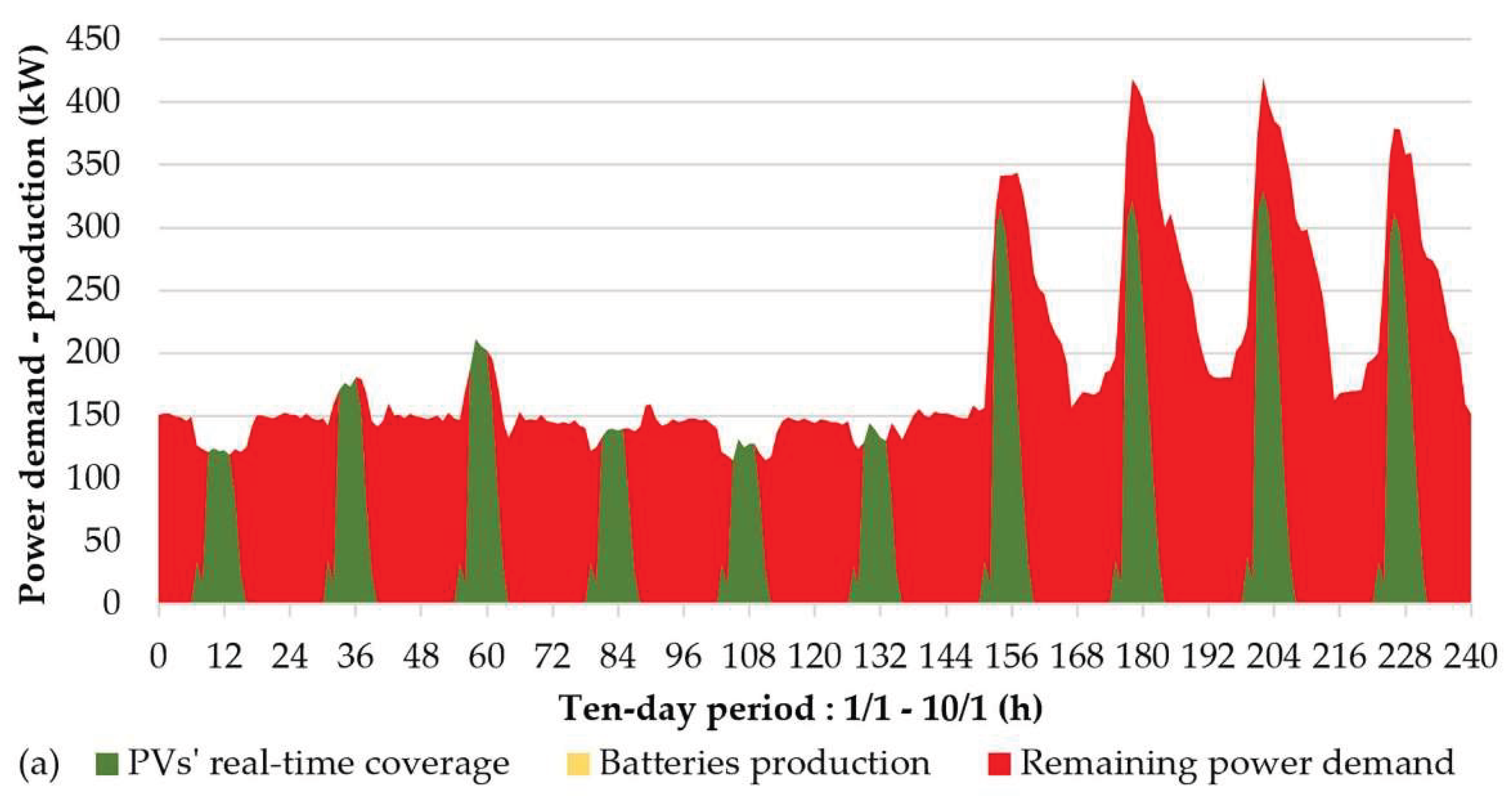
Figure 23.
b. Power demand and production fluctuation from the 1st to the 10th of January for the HMU main campus and the 7th investigated sizing scenario (2000 kWp PVs / 4000 kWh storage capacity).
Figure 23.
b. Power demand and production fluctuation from the 1st to the 10th of January for the HMU main campus and the 7th investigated sizing scenario (2000 kWp PVs / 4000 kWh storage capacity).
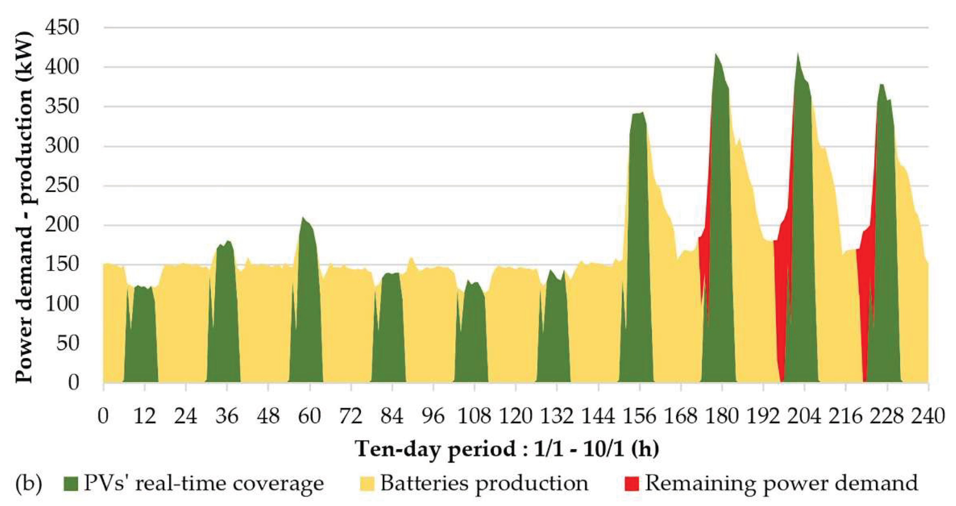
Figure 23a and Figure 23b refers to the HMU. The lower power demand in the first days of year, due to the Christmas holiday season, is totally covered by the photovoltaic – storage plant. During the normal operation of the institute (from the 8th of January and on), the electricity stored in the batteries is not enough to fully undertake the power demand during the early morning hours, just before the beginning of the new photovoltaic power production after sunrise. In the investigated scenario without storage support, all photovoltaics’ production is compensated with the concurrent power demand. Due to the low PVs’ nominal power (500 kWp) there is no photovoltaic production surplus in the specific time period. In Figure 23a and Figure 23b, the importance of the temporal coincidence of the peak power demand period with the photovoltaic power production is revealed, with regard to the maximization of the real-time power demand coverage.
Figure 24.
a. Power demand and production fluctuation from the 1st to the 10th of July for the Crete Aquarium and the 1st investigated sizing scenario (1000 kWp PVs / 0 kWh storage capacity).
Figure 24.
a. Power demand and production fluctuation from the 1st to the 10th of July for the Crete Aquarium and the 1st investigated sizing scenario (1000 kWp PVs / 0 kWh storage capacity).
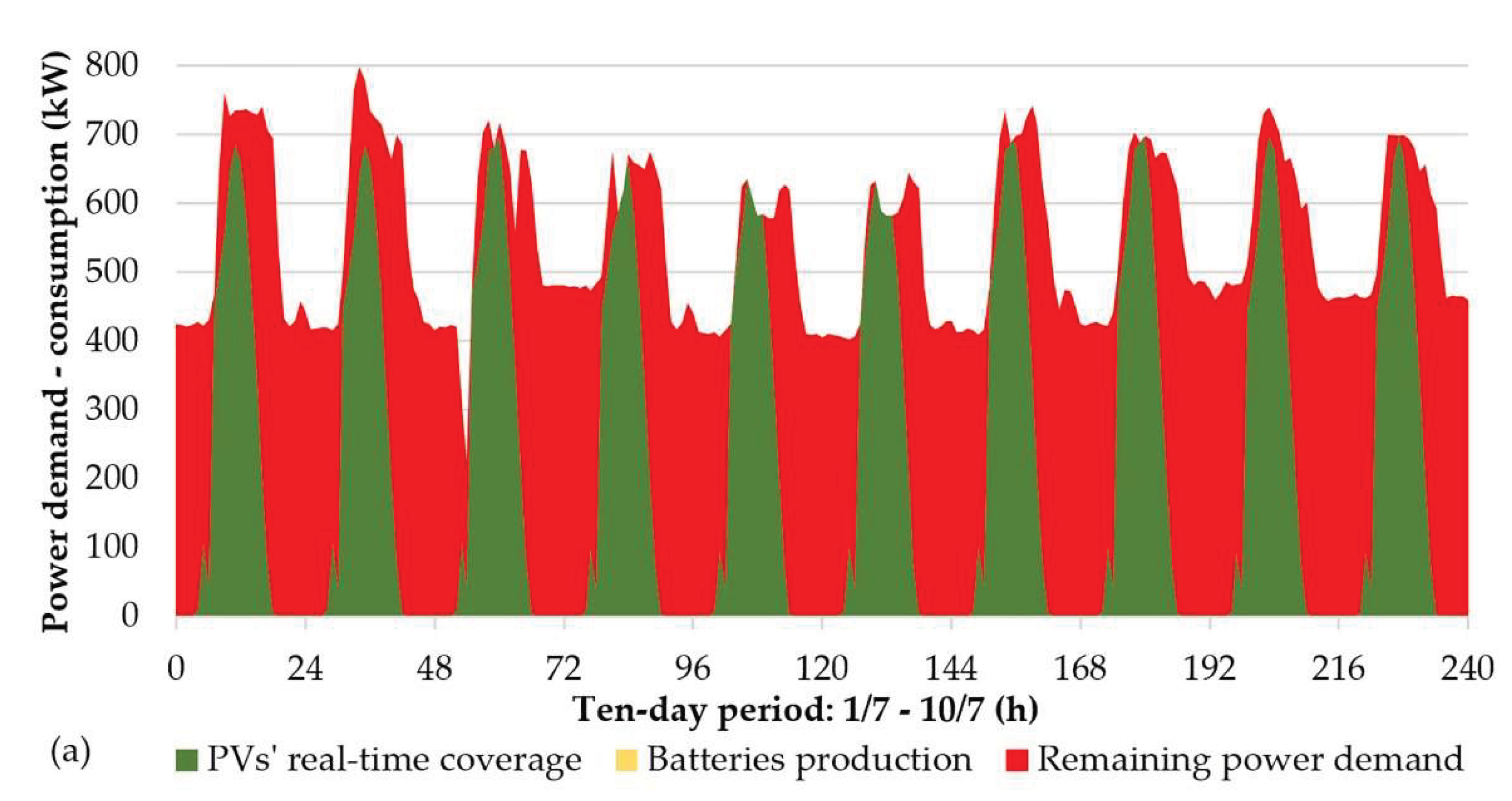
Figure 24.
b. Power demand and production fluctuation from the 1st to the 10th of July for the Crete Aquarium and the 8th investigated sizing scenario (3000 kWp PVs / 8000 kWh storage capacity).
Figure 24.
b. Power demand and production fluctuation from the 1st to the 10th of July for the Crete Aquarium and the 8th investigated sizing scenario (3000 kWp PVs / 8000 kWh storage capacity).
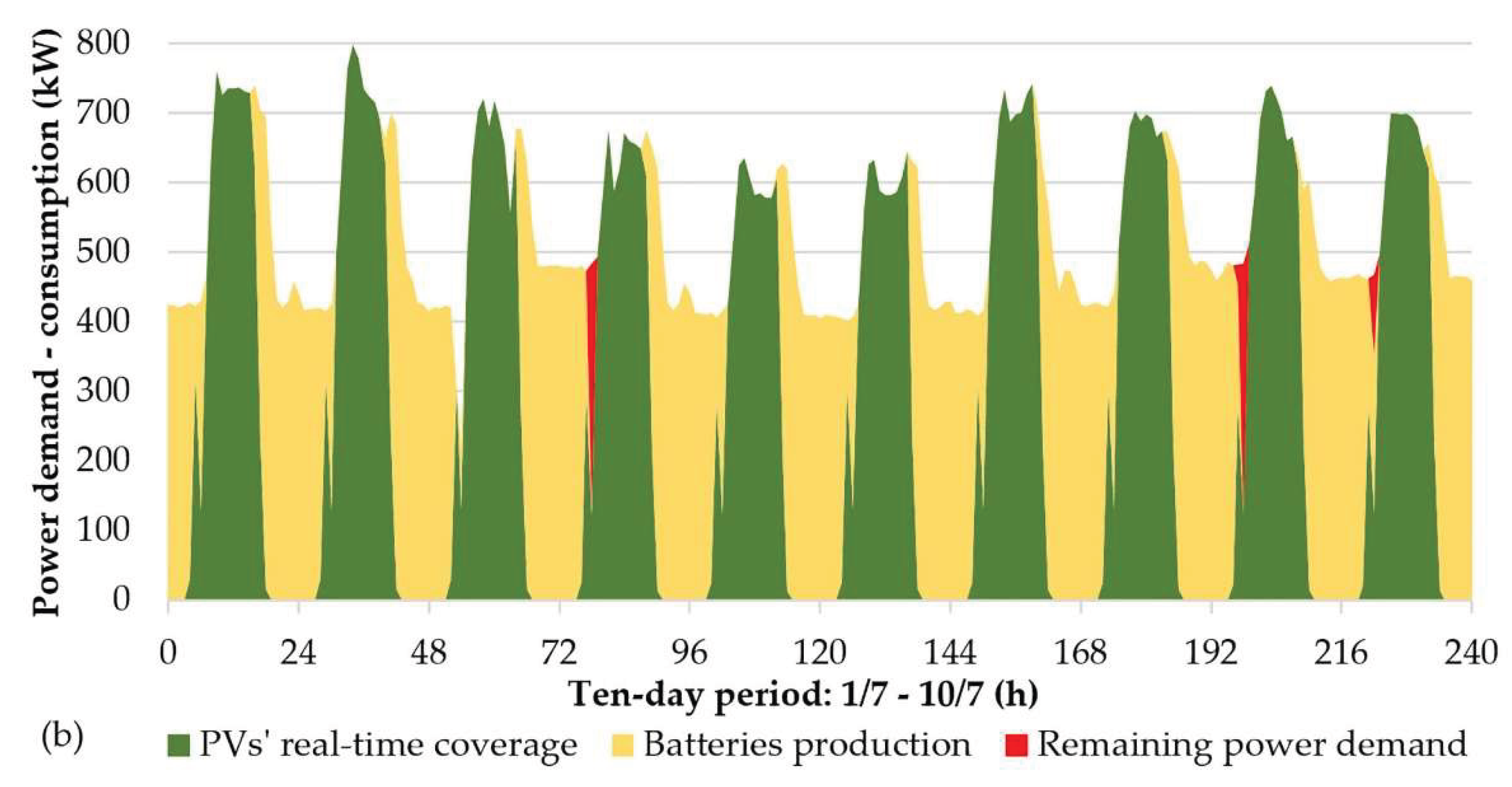
By observing Figure 24a and Figure 24b we may conclude to similar remarks for the case of the Crete Aquarium, as with HMU. The depicted time period falls into the annual peak power demand period, due to the summer tourist season. Photovoltaic production is restricted only during daytime in the first scenario, without storage support. The relatively low installed PVs power (1000 kWp), with regard to the power demand scale, leads to almost full exploitation of the photovoltaic production, with almost null production surplus. In the second scenario, the high incident solar irradiance, combined with the adequate storage capacity enables the almost full real time coverage of the power demand.
Figure 25.
a. Power demand and production fluctuation from the 21st to the 30th of May for the aluminum frames factory and the 1st investigated sizing scenario (50 kWp PVs / 0 kWh storage capacity).
Figure 25.
a. Power demand and production fluctuation from the 21st to the 30th of May for the aluminum frames factory and the 1st investigated sizing scenario (50 kWp PVs / 0 kWh storage capacity).
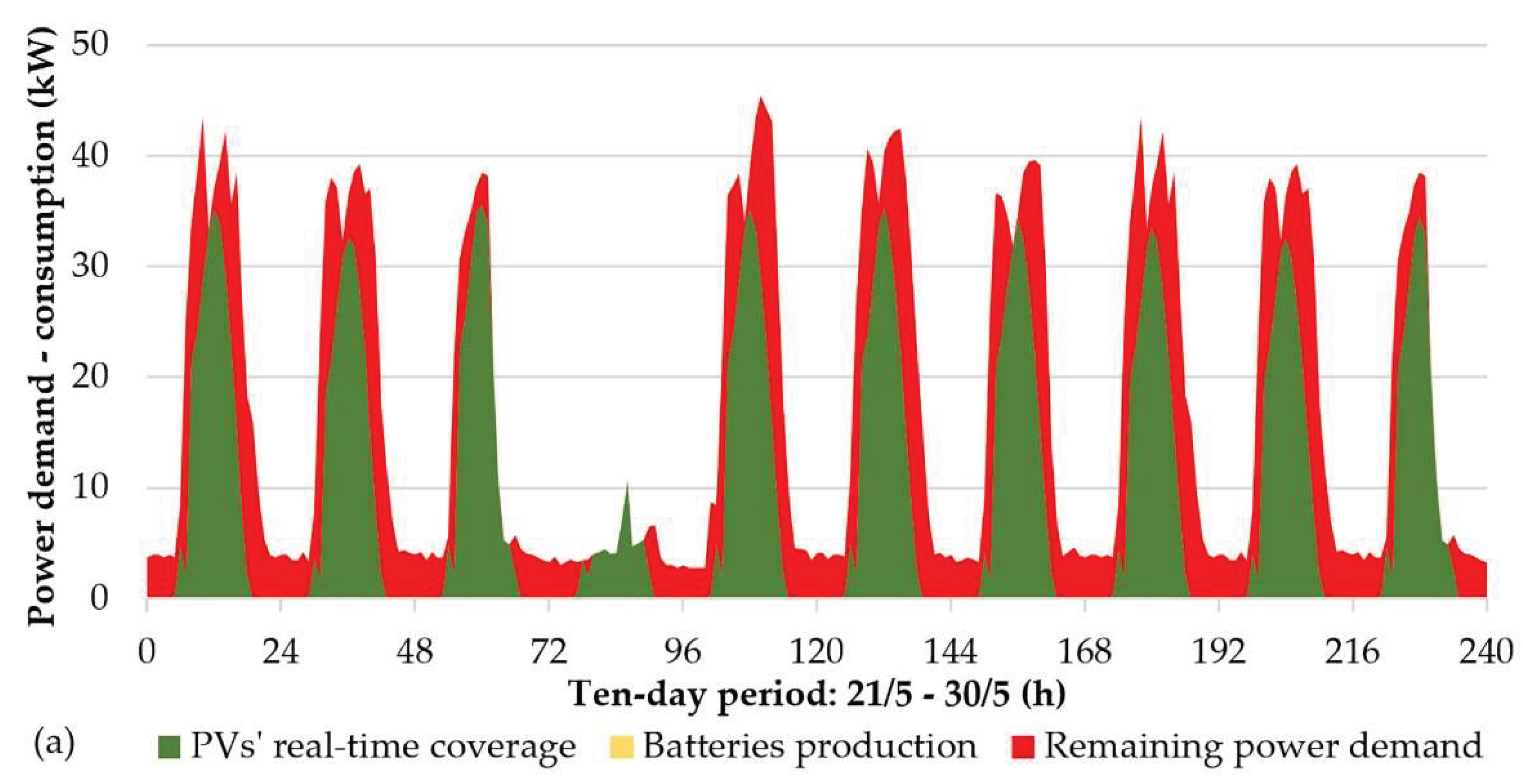
Figure 25.
b. Power demand and production fluctuation from the 21st to the 30th of May for the aluminum frames factory and the 5th investigated sizing scenario (150 kWp PVs / 200 kWh storage capacity).
Figure 25.
b. Power demand and production fluctuation from the 21st to the 30th of May for the aluminum frames factory and the 5th investigated sizing scenario (150 kWp PVs / 200 kWh storage capacity).
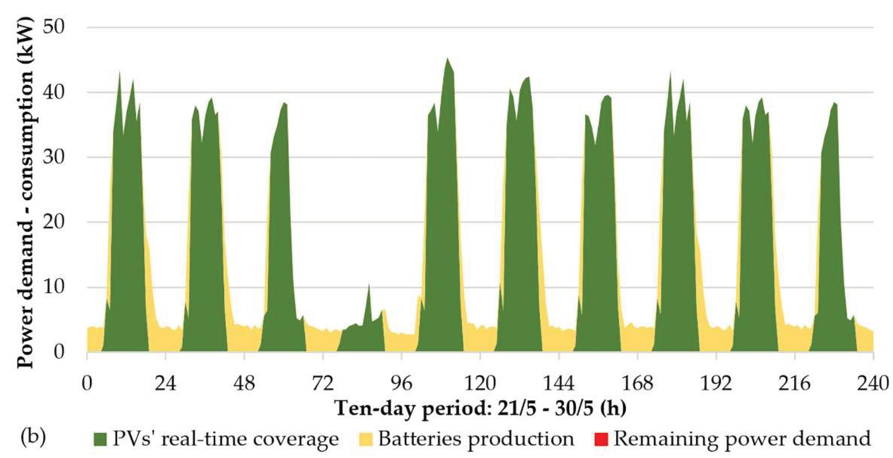
For the case of the aluminum frames manufacturing factory, depicted in Figure 25a and Figure 25b, the importance of the temporal coincidence between the photovoltaic power production and peak power demand on the achievement of high real-time power demand coverage is clearly revealed. Due to this fast, in the second investigated scenario, all power demand is compensated during daytime exclusively by the photovoltaics’ production. The storage support is limited only during nighttime.
Figure 26.
a. Power demand and production fluctuation from the 1st to the 10th of January for the 100 households group and the 1st investigated sizing scenario (200 kWp PVs / 0 kWh storage capacity).
Figure 26.
a. Power demand and production fluctuation from the 1st to the 10th of January for the 100 households group and the 1st investigated sizing scenario (200 kWp PVs / 0 kWh storage capacity).
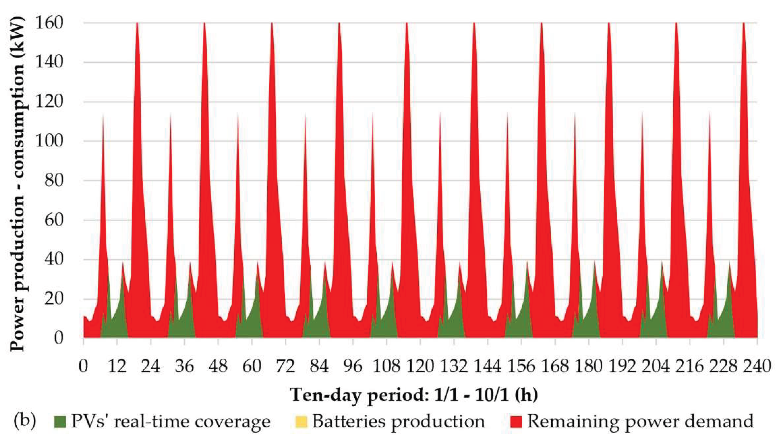
Figure 26.
b. Power demand and production fluctuation from the 1st to the 10th of January for the 100 households group and the 6th investigated sizing scenario (500 kWp PVs / 1000 kWh storage capacity).
Figure 26.
b. Power demand and production fluctuation from the 1st to the 10th of January for the 100 households group and the 6th investigated sizing scenario (500 kWp PVs / 1000 kWh storage capacity).
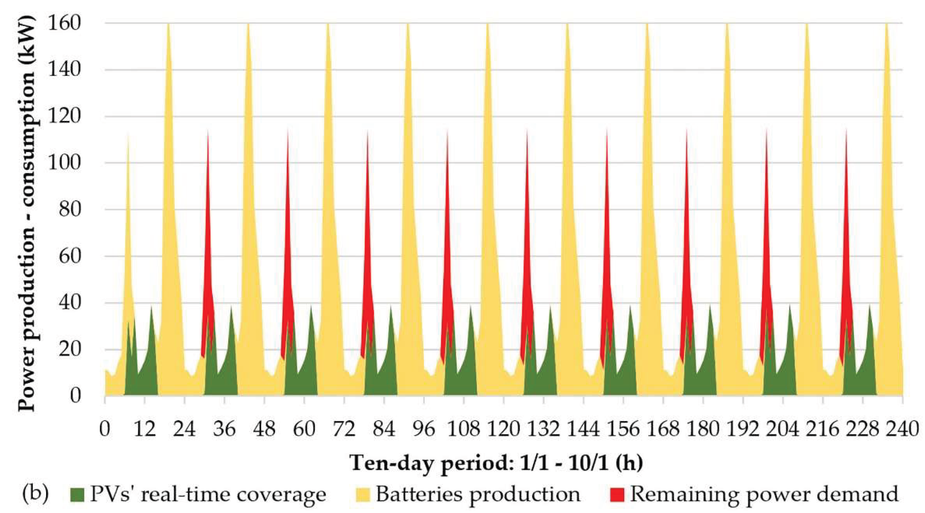
Unlike the previously investigated facilities, in the case of the households the low power demand during daytime restricts considerably the direct PVs’ production contribution to the power demand real-time coverage. The role of the batteries is maximized. The electricity demand compensation without storage support (first scenario depicted in Figure 26a) is remarkably low. With storage support, power demand is not compensated only during the early morning hours, just before sunrise. It should, however, be underlined, that in the winter time period depicted in Figure 26a and Figure 26b the incident solar irradiance is lower than 50% compared to the summer conditions (see Figure 14 in Section 3.2.1), hence the operation conditions of this specific period do not favor the achievement of full power demand real-time compensation.
Figure 27.
a. Power demand and production fluctuation from the 1st to the 10th of July for the travel agency and the 1st investigated sizing scenario (5 kWp PVs / 0 kWh storage capacity).
Figure 27.
a. Power demand and production fluctuation from the 1st to the 10th of July for the travel agency and the 1st investigated sizing scenario (5 kWp PVs / 0 kWh storage capacity).
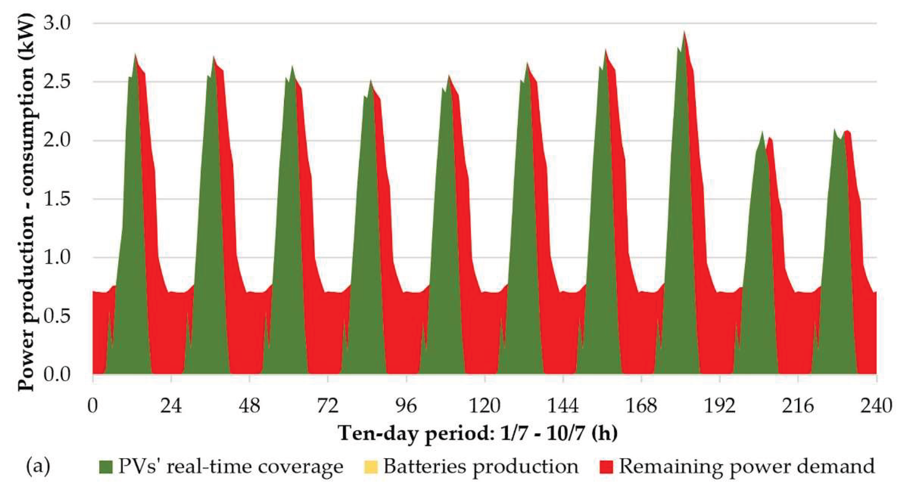
Figure 27.
b. Power demand and production fluctuation from the 1st to the 10th of July for the travel agency and the 5th investigated sizing scenario (10 kWp PVs / 15 kWh storage capacity).
Figure 27.
b. Power demand and production fluctuation from the 1st to the 10th of July for the travel agency and the 5th investigated sizing scenario (10 kWp PVs / 15 kWh storage capacity).
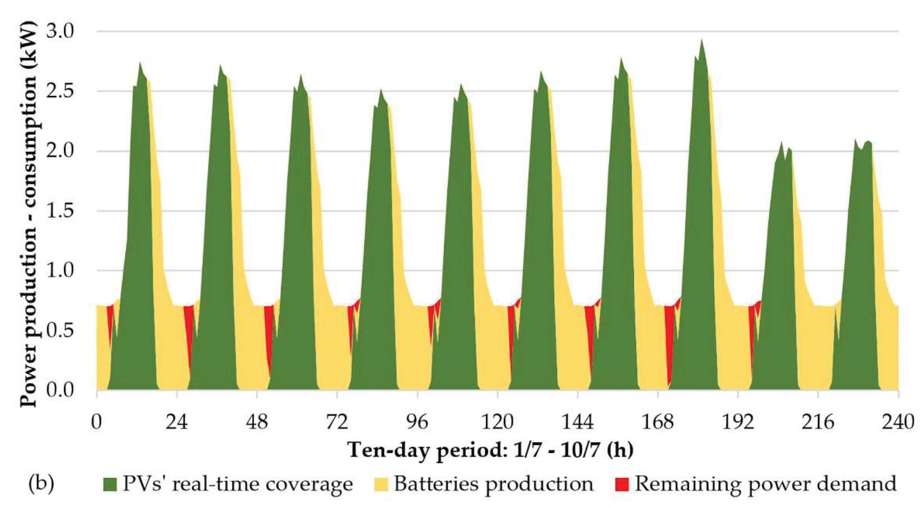
Finally, in the case of the travel agency, the peak power demand coincides with the photovoltaic power production, leading to high real-time direct power demand compensation from the PVs’ production. Despite the increased power demand during the depicted in Figure 27a and Figure 27b time period in July, power demand is not compensated only during the early morning hours, just before sunrise, thanks to the high incident solar irradiance and the adequate storage capacity, which is enough to fully undertake even the considerable base load during nighttime of the facility.
5. Discussion
The results demonstrate that the effectiveness of photovoltaic self-production depends strongly on the temporal alignment between electricity demand and solar generation. Within the common climatic setting examined, differences in operating schedules and system sizing produce markedly different demand coverage and surplus generation outcomes. High solar availability therefore provides favorable conditions for self-production, but does not alone ensure efficient utilisation of the installed capacity. Furthermore, because surplus electricity generates no revenue in the adopted assessment, the findings concern the value of avoided electricity purchases rather than the full range of potential revenues under net billing.
The distinction between demand coverage and photovoltaic self-consumption is essential when interpreting these outcomes. Demand coverage expresses the fraction of consumption supplied by photovoltaics and batteries, whereas self-consumption concerns the utilisation of photovoltaic generation. The Aquarium illustrates this distinction: its smallest photovoltaic configuration leaves only 7.6% of generation unused, although substantial electricity imports remain necessary. Consequently, effective utilisation of photovoltaic production does not necessarily imply high consumer self-sufficiency. This distinction also limits direct numerical comparisons with the self-consumption percentages reported in previous studies [40,49].
Operating schedules explain important differences among consumers. Daytime industrial activity supports direct photovoltaic demand coverage of 47.0–65.6% in the examined configurations without storage. HMU demand also coincides with solar production, although weekends and holiday closures reduce consumption during available generation periods. The Aquarium benefits from continuous operation and increased summer demand, while the travel agency combines daytime activity with a persistent nighttime base load. Conversely, residential morning and evening peaks limit direct coverage to 25.0–30.1%. These findings reinforce the importance of demand profiles identified in previous investigations [48,49], while showing that daily coincidence must be considered alongside seasonal demand and periods of inactivity.
Increasing photovoltaic capacity without corresponding flexibility produces diminishing returns. At HMU, doubling capacity from 500 to 1000 kWp increases demand coverage from 34.7% to 43.3%, while surplus generation rises from 15.7% to 47.3%. The residential case is more pronounced: increasing capacity from 200 to 500 kWp raises coverage by only 5.1 percentage points, with surplus reaching 85.8%. Sizing installations primarily to match annual electricity consumption can therefore substantially overestimate the usefulness of additional generation when demand and production are poorly aligned.
Storage changes this relationship by transferring surplus daytime production to subsequent demand periods. Suitable photovoltaic–battery combinations achieve reported annual coverage above 90% across all five cases. Nevertheless, high coverage can coexist with substantial unused generation. For example, the industrial configuration achieving 96.0% coverage still leaves 41.8% of photovoltaic production unused. Batteries therefore alleviate temporal mismatch without necessarily eliminating it, particularly when generation exceeds both concurrent demand and available storage capacity. Moreover, high annual coverage should not be interpreted as continuous autonomy or demonstrated outage resilience, neither of which is established by the annual energy balance.
The residential scenarios provide a particularly clear illustration of the importance of joint sizing. A 300 kWp photovoltaic installation with 1000 kWh of storage achieves 92.9% demand coverage, with 21.6% surplus and a 7.4-year simple payback. Increasing photovoltaic capacity to 500 kWp with unchanged storage raises coverage to 97.5%, but surplus increases to 50.7% and payback extends to 9.3 years. These results indicate that accepting a modest residual grid contribution can substantially reduce investment requirements and unused generation. The configurations examined establish useful trade-offs, although they do not constitute a continuous optimization demonstrating a unique optimum.
The economic effect of batteries is not uniform. For most non-residential configurations, higher coverage requires longer payback than the smallest photovoltaic-only installation, consistent with the trade-offs discussed in studies [47,49,50]. However, residential storage can also improve whole-system payback: adding 500 kWh to the 200 kWp installation increases coverage from 25.0% to 61.7% and reduces payback from 7.9 to 6.8 years. This exception reflects the large quantity of otherwise unused residential photovoltaic generation. Whole-system payback should nevertheless be distinguished from the incremental return on the battery investment, which requires comparing its additional cost with its additional savings.
The financial indicators remain conditional on the adopted assumptions. Simple payback excludes financing and discounting, while the electricity coverage specific cost is a capital-based indicator rather than a comprehensive levelized cost incorporating maintenance, degradation and replacements. Comparisons also depend on the evaluation horizon, particularly the 25-year lifespan assigned to the largest Aquarium storage configuration or single photovoltaics installations (no storage) versus 15 years for most battery systems. Applying average procurement prices to displaced electricity further assumes that these prices represent avoidable charges. Consumer-specific tariffs and separation of fixed and variable costs would improve the savings estimates.
Several modelling limitations warrant further investigation. Hourly averages may conceal shorter demand–generation mismatches. Residential profiles are synthesised from repeated daily patterns, while the commercial series is reconstructed from limited measurement periods. The use of clear-sky irradiance also requires validation against actual cloud-affected conditions, and wind measurements are not contemporaneous with the remaining meteorological inputs. These features constrain extrapolation to other consumers and Mediterranean locations. Future work should combine multi-year, higher-resolution measurements with battery degradation, explicit power constraints and discounted economic assessment. Demand response and complementary load sharing, motivated by earlier community studies [34,48], should also be examined as possible means of reducing storage requirements before pursuing further photovoltaic expansion.
6. Conclusions
This study assessed photovoltaic self-production, with and without electrochemical storage, for five consumer categories under the climatic conditions considered for Crete, Greece. The results show that temporal coincidence between electricity consumption and photovoltaic generation is central to both demand coverage and investment performance. Annual consumption alone is therefore insufficient for selecting photovoltaic capacity.
Without storage, the examined configurations achieve direct annual demand coverage of 34.7–43.3% at HMU, 34.6–36.4% at the Aquarium, 47.0–65.6% at the industrial facility and 45.4–51.4% at the travel agency. Residential coverage remains lower, at 25.0–30.1%, because demand is concentrated outside peak solar production hours. Increasing photovoltaic capacity improves coverage, but can substantially increase unused generation when additional output cannot coincide with consumption.
Appropriate combinations of photovoltaic capacity and storage achieve reported annual demand coverage above 90% in every case study. However, maximising coverage does not necessarily yield the most attractive economic configuration. The residential installation comprising 300 kWp of photovoltaics and 1000 kWh of storage illustrates a favorable compromise among the examined alternatives, achieving 92.9% coverage, 21.6% surplus generation and a 7.4-year simple payback. Further photovoltaic expansion produces comparatively small coverage gains at higher investment cost.
Storage generally extends whole-system payback relative to smaller photovoltaic-only installations, but this outcome is not universal. Where the initial temporal mismatch is pronounced, batteries can recover sufficient unused generation to improve both coverage and payback, as demonstrated by the residential 200 kWp configuration.
The main design implication is that photovoltaic and battery capacities should be selected jointly according to consumer demand profiles, acceptable residual grid dependence and economic objectives. The reported outcomes remain conditional on the meteorological inputs, reconstructed demand profiles, tariff assumptions and simplified financial evaluation. Validation using measured, multi-year data and comprehensive lifecycle costs would strengthen investment decisions and establish the transferability of the findings to other Mediterranean consumers.
Author Contributions
Conceptualization, D.K.; methodology, D.K.; software, D.K. and N.P.; validation, D.K., N.P. and G.V.; formal analysis, N.K. and G.V.; investigation, D.K. and N.K.; resources, I.P. and M.L.; data curation, D.K. and M.L.; writing—original draft preparation, D.K., N.P. and N.K.; writing—review and editing, D.K.; visualization, D.K.; supervision, D.K.; project administration, D.K.; funding acquisition, D.K., G.P. and M.L. All authors have read and agreed to the published version of the manuscript.
Funding
This research was partially funded by the Hellenic Centre of Marine Research, under a private bilateral grant number with the consulting firm Aeolian Land S.A.
Data Availability Statement
The data presented in this study are available on request from the corresponding author due to privacy reasons.
Acknowledgments
The authors are grateful to the Hellenic Centre of Marine Research for the partial funding of this work.
Conflicts of Interest
The authors declare no conflicts of interest.
Abbreviations
The following abbreviations are used in this manuscript:
| RES | Renewable Energy Sources |
| ESS | Energy storage systems |
| PHS | Pumped Hydro Storage |
| CAES | Compressed Air Energy Storage |
| PVs | photovoltaic plants |
| BESS | Battery Energy Storage Systems |
| HMU | Hellenic Mediterranean University |
| ECMWF | European Centre for Medium-Range Weather Forecasts |
References
- Adinkrah, J.; Kemausuor, F.; Tutu Tchao, E.; Nunoo-Mensah, H.; Agbemenu, A.S.; Adu-Poku, A.; Kponyo, J.J. Artificial intelligence-based strategies for sustainable energy planning and electricity demand estimation: A systematic review. Renew. Sustain. Energy Rev. 2025, 210, 115161. [Google Scholar] [CrossRef]
- Lelieveld, J.; Haines, A.; Burnett, R.; Tonne, C.; Klingmüller, K.; Münzel, T.; Pozzer, A. Air pollution deaths attributable to fossil fuels: observational and modelling study. BMJ 2023, 383, e077784. [Google Scholar] [CrossRef]
- Filonchyk, M.; Peterson, M.P.; Zhang, L.; Hurynovich, V.; He, Y. Greenhouse gases emissions and global climate change: Examining the influence of CO2, CH4, and N2O. Sci. Total Environ. 2024, 935, 173359. [Google Scholar] [CrossRef]
- Kim, J.; Jaumotte, F.; Panton, A.J.; Schwerhoff, G. Energy security and the green transition. Energy Policy 2025, 198, 114409. [Google Scholar] [CrossRef]
- Arnaoutakis, G.E.; Katsaprakakis, D.A. Energy Yield of Spectral Splitting Concentrated Solar Power Photovoltaic Systems. Energies 2024, 17(3), 556. [Google Scholar] [CrossRef]
- Atiea, M.A.; Abdelghaffar, A.A.; Aribia, H.B.; Noureddine, F.; Shaheen, A.M. Photovoltaic power generation forecasting with Bayesian optimization and stacked ensemble learning. Results Eng. 2025, 26, 104950. [Google Scholar] [CrossRef]
- Katsaprakakis, D.A.; Christakis, D.G. A Wind Parks, Pumped Storage and Diesel Engines Power System for the electric power production in Astypalaia. In Proceedings of the European Wind Energy Conference and Exhibition 2006, Athens, Greece, 27 February to 2 March 200; pp. 621–636.
- Katsaprakakis, D.A.; Christakis, D.G. Maximisation of R.E.S. penetration in Greek insular isolated power systems with the introduction of pumped storage systems. In the Proceedings of the European Wind Energy Conference and Exhibition 2009, Marseille, France, 16–19 March 2009; pp. 4918–4930. [Google Scholar]
- Li, Y.; Peng, T.; Zhang, C.; Sun, W.; Hua, L.; Ji, C.; Muhammad Shahzad, N. Multi-step ahead wind speed forecasting approach coupling maximal overlap discrete wavelet transform, improved grey wolf optimization algorithm and long short-term memory. Renew. Energy 2022, 196, 1115–1126. [Google Scholar] [CrossRef]
- Rashid, T.H.M.S.; Refat, K.A.; Islam, M.N.; Khan, R.; Mostofa, E.M.R.; Hossain, M.A.; Kabir, H.; Ali, M.F. Machine learning-driven PV forecasting and coordinated PV–BESS dispatch for optimizing distribution grid performance under high EV penetration. Energy Convers. Manag. X 2026, 29, 101418. [Google Scholar] [CrossRef]
- Al-Hanahi, B.; Aziz, A. Community energy storage: A framework for enhanced energy trading and cost efficiency. J. Energy Storage 2026, 166, 122233. [Google Scholar] [CrossRef]
- Dogan, A.; Cidem Dogan, D. A Review on Machine Learning Models in Forecasting of Virtual Power Plant Uncertainties. Arch. Comput. Methods Eng. 2023, 30(3), 2081–2103. [Google Scholar] [CrossRef]
- Fotopoulou, M.; Pediaditis, P.; Skopetou, N.; Rakopoulos, D.; Christopoulos, S.; Kartalidis, A. A Review of the Energy Storage Systems of Non-Interconnected European Islands. Sustainability 2024, 16(4), 1572. [Google Scholar] [CrossRef]
- Caralis, G.; Christakopoulos, T.; Karellas, S.; Gao, Z. Analysis of energy storage systems to exploit wind energy curtailment in Crete. Renew. Sustain. Energy Rev. 2019, 103, 122–139. [Google Scholar] [CrossRef]
- Liu, T.; Yang, Z.; Duan, Y. Short- and long-duration cooperative energy storage system: Optimizing sizing and comparing rule-based strategies. Energy 2023, 281, 128273. [Google Scholar] [CrossRef]
- Kallitsounakis, N.E.; Katsaprakakis, D.A.; Condaxakis, C.; Papadakis, N. Technical and economic parameters regarding the operation of wind parks and pumped hydro storage systems in autonomous and in interconnected insular electrical systems. J. Energy Storage 2026, 153, 120999. [Google Scholar] [CrossRef]
- Arnaoutakis, G.E.; Kocher-Oberlehner, G.; Katsaprakakis, D.A. Criteria-Based Model of Hybrid Photovoltaic–Wind Energy System with Micro-Compressed Air Energy Storage. Mathematics 2023, 11(2), 391. [Google Scholar] [CrossRef]
- Aranzabal, I.; Gomez-Cornejo, J.; López, I.; Zubiria, A.; Mazón, J.; Feijoo-Arostegui, A.; Gaztañaga, H. Optimal Management of an Energy Community with PV and Battery-Energy-Storage Systems. Energies 2023, 16(2), 789. [Google Scholar] [CrossRef]
- Pompodakis, E.E.; Ahmed, A.; Condaxakis, C.; Orfanoudakis, G.I.; Karapidakis, E.S. Paving the way toward hydrogen mobility: An effective policy to reduce the green hydrogen cost. Int. J. Hydrogen Energy 2025, 100, 417–427. [Google Scholar] [CrossRef]
- Zheng, Y.; Wang, J.; You, S.; Li, X.; Bindner, H.W.; Münster, M. Data-driven scheme for optimal day-ahead operation of a wind/hydrogen system under multiple uncertainties. Appl. Energy 2023, 329, 120201. [Google Scholar] [CrossRef]
- Abdon, A.; Zhang, X.; Parra, D.; Patel, M.K.; Bauer, C.; Worlitschek, J. Techno-economic and environmental assessment of stationary electricity storage technologies for different time scales. Energy 2017, 139, 1173–1187. [Google Scholar] [CrossRef]
- Katsaprakakis, D.A. Toward a Renewable and Sustainable Energy Pattern in Non-Interconnected Rural Monasteries: A Case Study for the Xenofontos Monastery, Mount Athos. Sustainability 2024, 16(5), 2111. [Google Scholar] [CrossRef]
- Tumminello, D.; Zuffi, C.; Bacci, T.; Facchini, B. Hybrid micro-compressed air energy storage with photovoltaic and diesel generation for off-grid applications: A parametric life cycle and techno-economic study. Clean. Energy Syst. 2026, 13, 100246. [Google Scholar] [CrossRef]
- Rosato, A.; Adamo, G.M.; Araneo, R.; Panella, M. A two-stage decision system based on distributed optimization in energy communities. Int. J. Electr. Power Amp Energy Syst. 2026, 176, 111734. [Google Scholar] [CrossRef]
- Ahmed, S.; Ali, A.; D’Angola, A. A Review of Renewable Energy Communities: Concepts, Scope, Progress, Challenges, and Recommendations. Sustainability 2024, 16(5), 1749. [Google Scholar] [CrossRef]
- Sousa, J.; Lagarto, J.; Camus, C.; Viveiros, C.; Barata, F.; Silva, P.; Alegria, R.; Paraíba, O. Renewable energy communities optimal design supported by an optimization model for investment in PV/wind capacity and renewable electricity sharing. Energy 2023, 283, 128464. [Google Scholar] [CrossRef]
- Rigo-Mariani, R.; Ahmed, A. Coordinated management under uncertainty and fair revenue distribution in a multi energy community. Energy 2025, 339, 138802. [Google Scholar] [CrossRef]
- Barone, G.; Buonomano, A.; Forzano, C.; Palombo, A.; Russo, G. The role of energy communities in electricity grid balancing: A flexible tool for smart grid power distribution optimization. Renew. Sustain. Energy Rev. 2023, 187, 113742. [Google Scholar] [CrossRef]
- Katsaprakakis, D.A.; Dakanali, E.; Dimopoulos, A.; Gkyllis, I. Energy Transition on Sifnos: An Approach to Economic and Social Transition and Development. Appl. Sci. 2022, 12(5), 2680. [Google Scholar] [CrossRef]
- Elomari, Y.; Mateu, C.; Marín-Genescà, M.; Boer, D. A data-driven framework for designing a renewable energy community based on the integration of machine learning model with life cycle assessment and life cycle cost parameters. Appl. Energy 2024, 358, 122619. [Google Scholar] [CrossRef]
- Pizzuti, I.; Delibra, G. Integration of battery energy storage systems in renewable energy communities: Optimal configurations and strategies. J. Energy Storage 2026, 153, 120857. [Google Scholar] [CrossRef]
- Sousa, J.; Perinhas, S.; Viveiros, C.; Barata, F. Increasing Economic Benefits in Renewable Energy Communities with Solar PV and Battery Storage Technologies: Insights from New Member Integration. Energies 2025, 18(18), 4815. [Google Scholar] [CrossRef]
- Chalkiadakis, G.; Akasiadis, C.; Savvakis, N.; Tsoutsos, T.; Hoppe, T.; Coenen, F. Providing a Scientific Arm to Renewable Energy Cooperatives. Role Exergy Energy Environ. 2018, 717–731. [Google Scholar] [CrossRef]
- dos Santos, S.A.B.; Coutinho, L.R.R.; Tofoli, F.L.; Barroso, G.C. Community energy management system for residential energy communities integrating demand response, distributed generation, and energy storage systems. J. Energy Storage 2025, 132, 117832. [Google Scholar] [CrossRef]
- Real, A.C.; Luz, G.P.; Sousa, J.M.C.; Brito, M.C.; Vieira, S.M. Optimization of a photovoltaic-battery system using deep reinforcement learning and load forecasting. Energy AI 2024, 16, 100347. [Google Scholar] [CrossRef]
- Dufo-López, R.; Bernal-Agustín, J.L. A comparative assessment of net metering and net billing policies. Study cases for Spain. Energy 2015, 84, 684–694. [Google Scholar] [CrossRef]
- Iliadis, P.; Ziozas, N.; Gonidaki, D.; Kitsopoulou, A.; Bellos, E.; Rotas, R.; Nikolopoulos, N.; Kosmatopoulos, E. Optimizing photovoltaic-battery systems for net-billing in Greece: Impact of building usage and pricing schemes. J. Build. Eng. 2026, 121, 115718. [Google Scholar] [CrossRef]
- Benalcazar, P.; Kalka, M.; Kamiński, J. Transitioning from net-metering to net-billing: A model-based analysis for Poland. Sustain. Energy Technol. Assess. 2024, 72, 104073. [Google Scholar] [CrossRef]
- Chatzigeorgiou, I.M.; Kitsikopoulos, D.; Papadaskalopoulos, D.A.; Chronis, A.G.; Xenaki, A.; Andreou, G.T. Optimal PV Sizing and Demand Response in Greek Energy Communities Under the New Virtual Net-Billing Scheme. Energies 2025, 18(19), 5082. [Google Scholar] [CrossRef]
- Simoglou, C.K.; Vagropoulos, S.I.; Biskas, P.N. A comparative techno-economic study of the Net-Metering and Net-Billing self-consumption schemes for industrial and residential consumers in Greece. Sustain. Energy Grids Netw. 2025, 43, 101726. [Google Scholar] [CrossRef]
- Miliarakis, S.; Tsakanikas, A. Assessing the economic feasibility of Li-ion batteries storage systems for electricity arbitrage: A case study of the Greek energy market. Next Res. 2025, 2(1), 100109. [Google Scholar] [CrossRef]
- An, J.; Hong, T. Multi-objective optimization for optimal placement of shared battery energy storage systems in urban energy communities. Sustain. Cities Soc. 2025, 120, 106178. [Google Scholar] [CrossRef]
- Pompodakis, E.E.; Kryonidis, G.C.; Karapidakis, E.S. Optimizing the installation of hybrid power plants in non-interconnected islands. J. Energy Storage 2023, 74, 109511. [Google Scholar] [CrossRef]
- Giannakopoulos, G.T.; Papadaskalopoulos, D.A.; Karasavvidis, M.D.; Vovos, P.N. Profitability Analysis of Battery Energy Storage in Energy and Balancing Markets: A Case Study in the Greek Market. Energies 2025, 18(4), 911. [Google Scholar] [CrossRef]
- Hodge, B.M.; Brancucci Martinez-Anido, C.; Wang, Q.; Chartan, E.; Florita, A.; Kiviluoma, J. The combined value of wind and solar power forecasting improvements and electricity storage. Appl. Energy 2018, 214, 1–15. [Google Scholar] [CrossRef]
- Psarros, G.N.; Papathanassiou, S.A. Electricity storage requirements to support the transition towards high renewable penetration levels – Application to the Greek power system. J. Energy Storage 2022, 55, 105748. [Google Scholar] [CrossRef]
- An, J.; Hong, T. Optimizing battery energy storage system placement in energy intensive cities for sustainable urban development considering multiple objectives. Sustain. Cities Soc. 2025, 118, 106036. [Google Scholar] [CrossRef]
- Chen, X.; Liu, Z.; Wang, P.; Li, B.; Liu, R.; Zhang, L.; Zhao, C.; Luo, S. Multi-objective optimization of battery capacity of grid-connected PV-BESS system in hybrid building energy sharing community considering time-of-use tariff. Appl. Energy 2023, 350, 121727. [Google Scholar] [CrossRef]
- Garabitos-Lara, E.; Vallejo-Díaz, A.; Pereyra-Mariñez, C.N.; Herrera-Moya, I. Techno-economic assessment of battery systems in the PV self-consumption without surpluses in the residential tariff of the Dominican Republic. Energy Sustain. Dev. 2026, 90, 101898. [Google Scholar] [CrossRef]
- Migliari, L.; Cocco, D. Cost-effectiveness of photovoltaic-battery systems for self-supply across various market and load conditions. J. Energy Storage 2025, 135, 118240. [Google Scholar] [CrossRef]
- European Centre for Medium-Range Weather Forecasts (ECMWF): ERA5 from the Copernicus Climate Change Service (C3S) Climate Date Store. ERA5 hourly data on single levels from 1959 to present. Available online: https://cds.climate.copernicus.eu/#!/search?text=ERA5&type=dataset (accessed on 4/9/2025).
- Karananos, A.; Dimara, A.; Arvanitis, K.; Timplalexis, C.; Krinidis, S.; Tzovaras, D. Energy Consumption Patterns of Residential Users: A Study in Greece. In the Proceedings of the International Conference on Computer Vision Systems. Lecture Notes in Computer Science (LNCS), Thessaloniki, Greece, 23–25 September 2019; Springer: Cham; 11754, pp. 639–650. [Google Scholar]
- International Electrotechnical Commission. IEC Standard No. 60904–3:2019; Photovoltaic devices - Part 3: Measurement principles for terrestrial photovoltaic (PV) solar devices with reference spectral irradiance data. 2019.
- Kreider, J.; Rabl, A.; Curtiss, P. Heating and Cooling of Buildings. 3rd Edition, 2017; CRC Press: Boca Raton, FL, USA.
- Fragkiadakis, I. Photovoltaic systems, 4th edition; Ziti Editions: Athens, 2019. [Google Scholar]
- Faiman, D. Assessing the outdoor operating temperature of photovoltaic modules. Prog. Photovolt. 2008, 16(4), 307–315. [Google Scholar] [CrossRef]
- IEC 61853-2; Photovoltaic (PV) module performance testing and energy rating - Part 2: Spectral responsivity, incidence angle and module operating temperature measurements. IEC: Geneva, 2018.
- IEC 61853-3; Photovoltaic (PV) module performance testing and energy rating - Part 3: Energy rating of PV modules. IEC: Geneva, 2018.
Figure 1.
Annual power demand fluctuation in the main campus of the Hellenic Mediterranean University in 2025.
Figure 1.
Annual power demand fluctuation in the main campus of the Hellenic Mediterranean University in 2025.
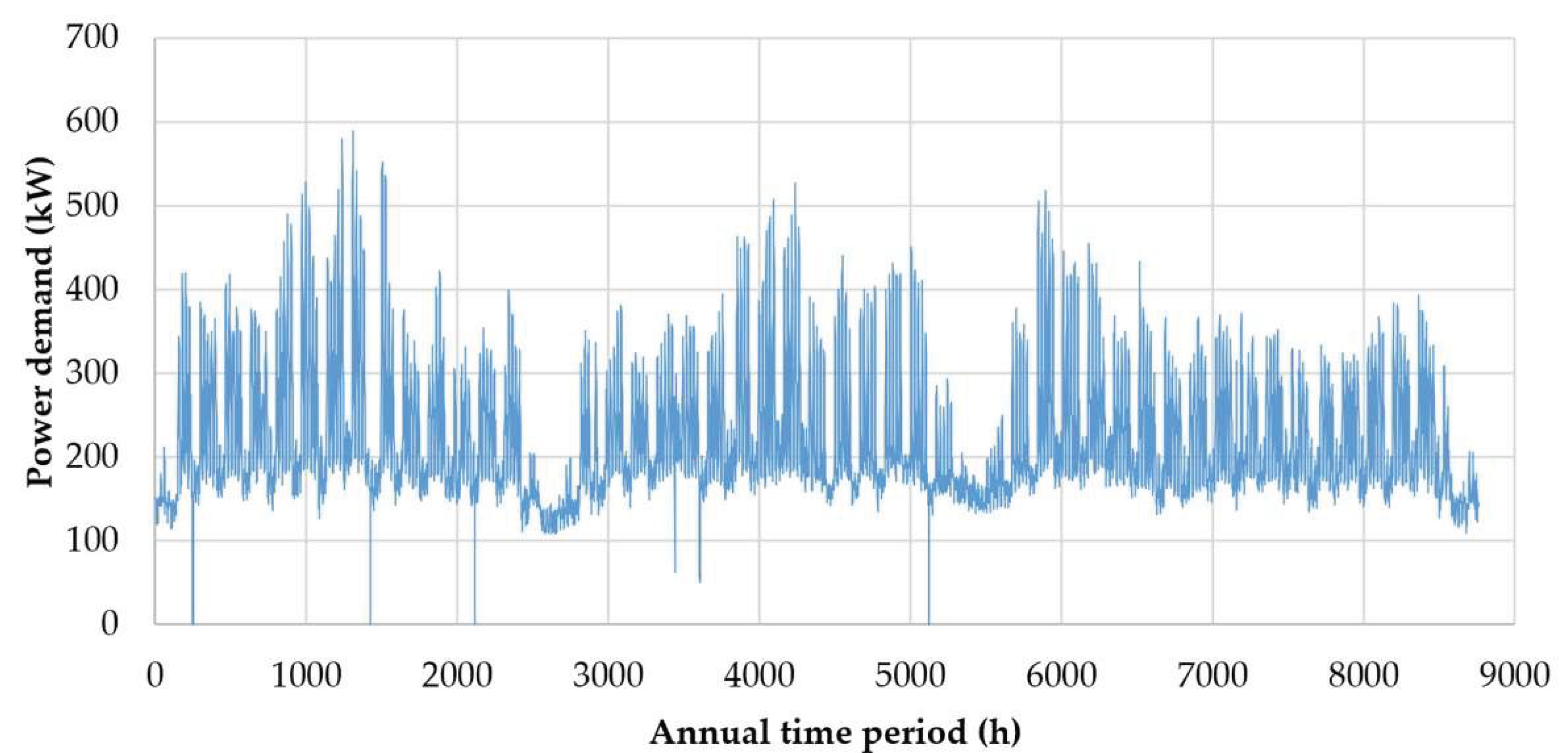
Figure 2.
Annual power demand fluctuation in the Crete Aquarium in 2025.
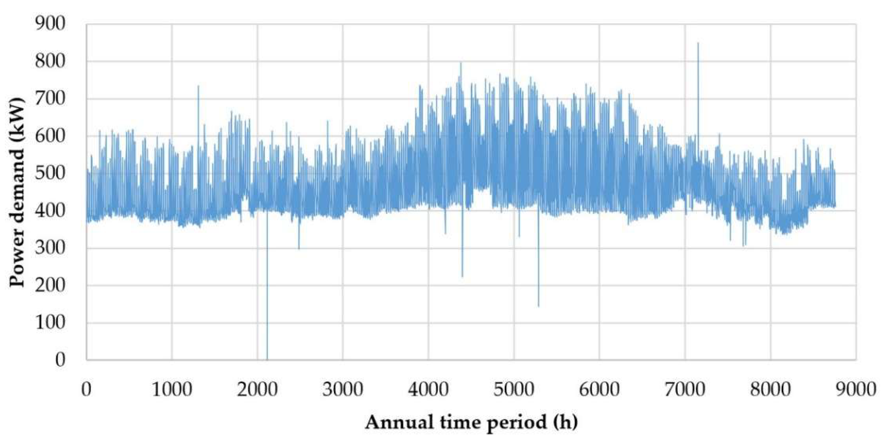
Figure 3.
Power demand fluctuation in the main campus of the HMU on the 11–20 February 2025.
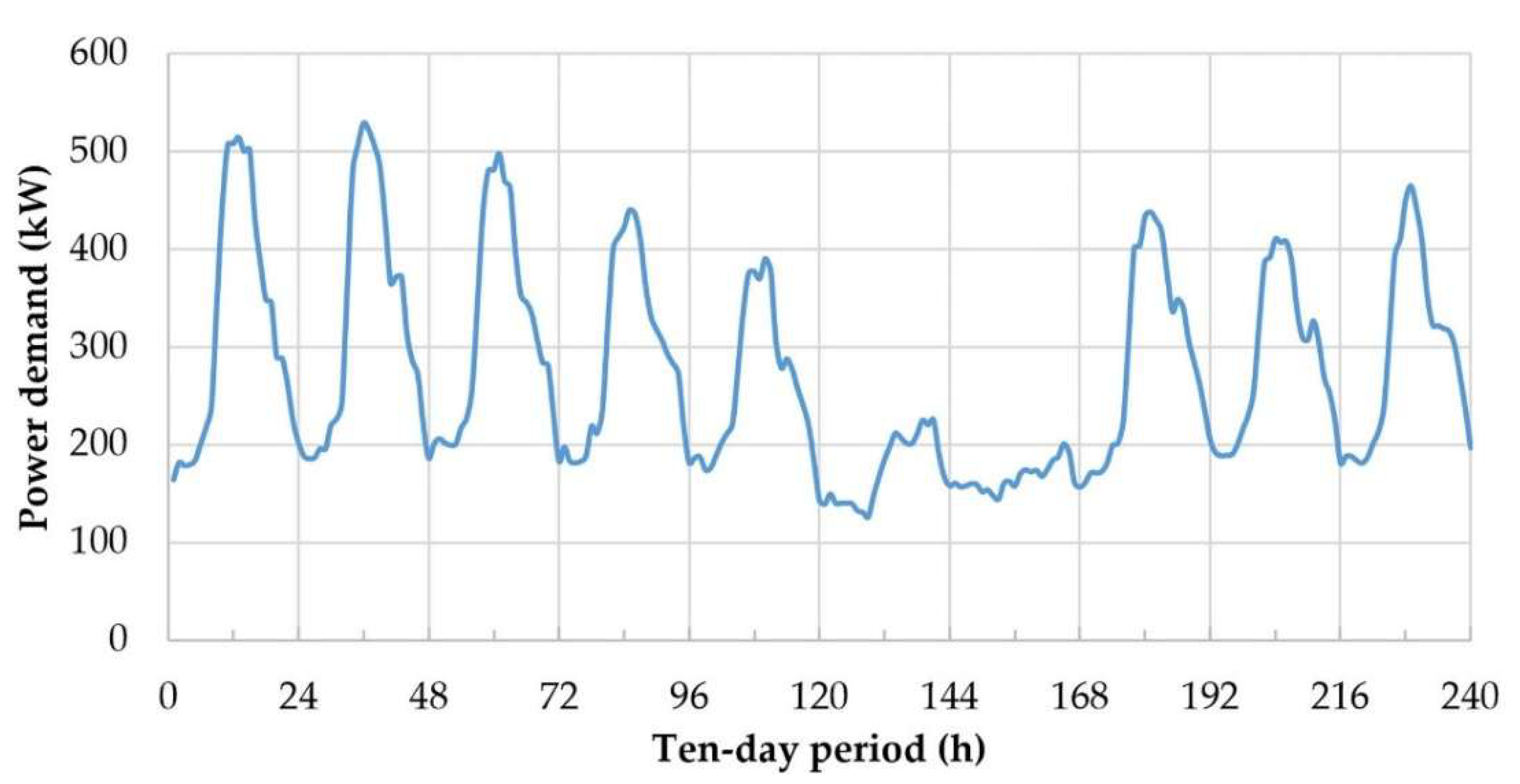
Figure 4.
Power demand fluctuation in the Crete Aquarium on 25 July – 4 August 2025.
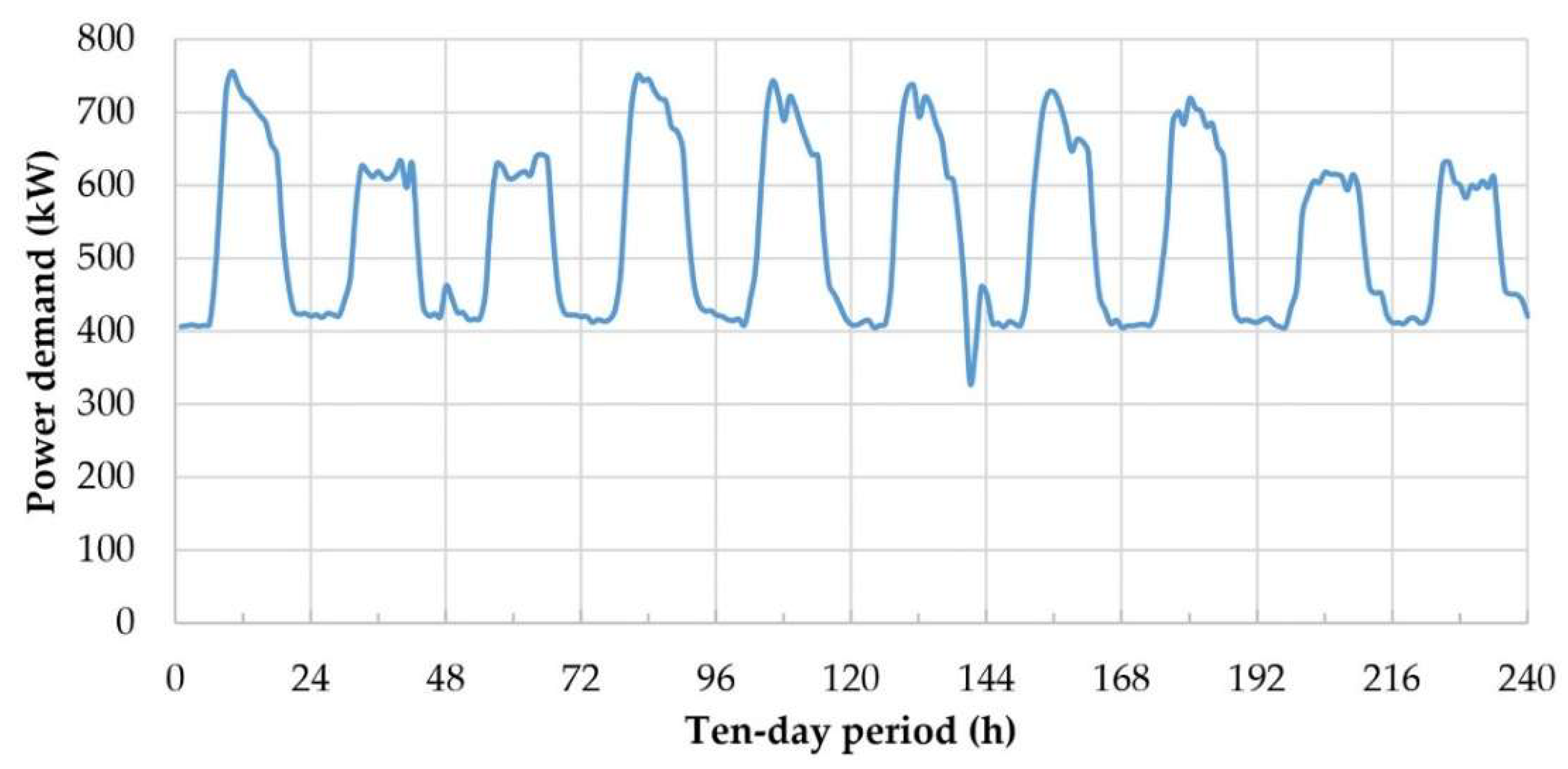
Figure 5.
Annual power demand fluctuation in the aluminum frames manufacturing factory in 2025.
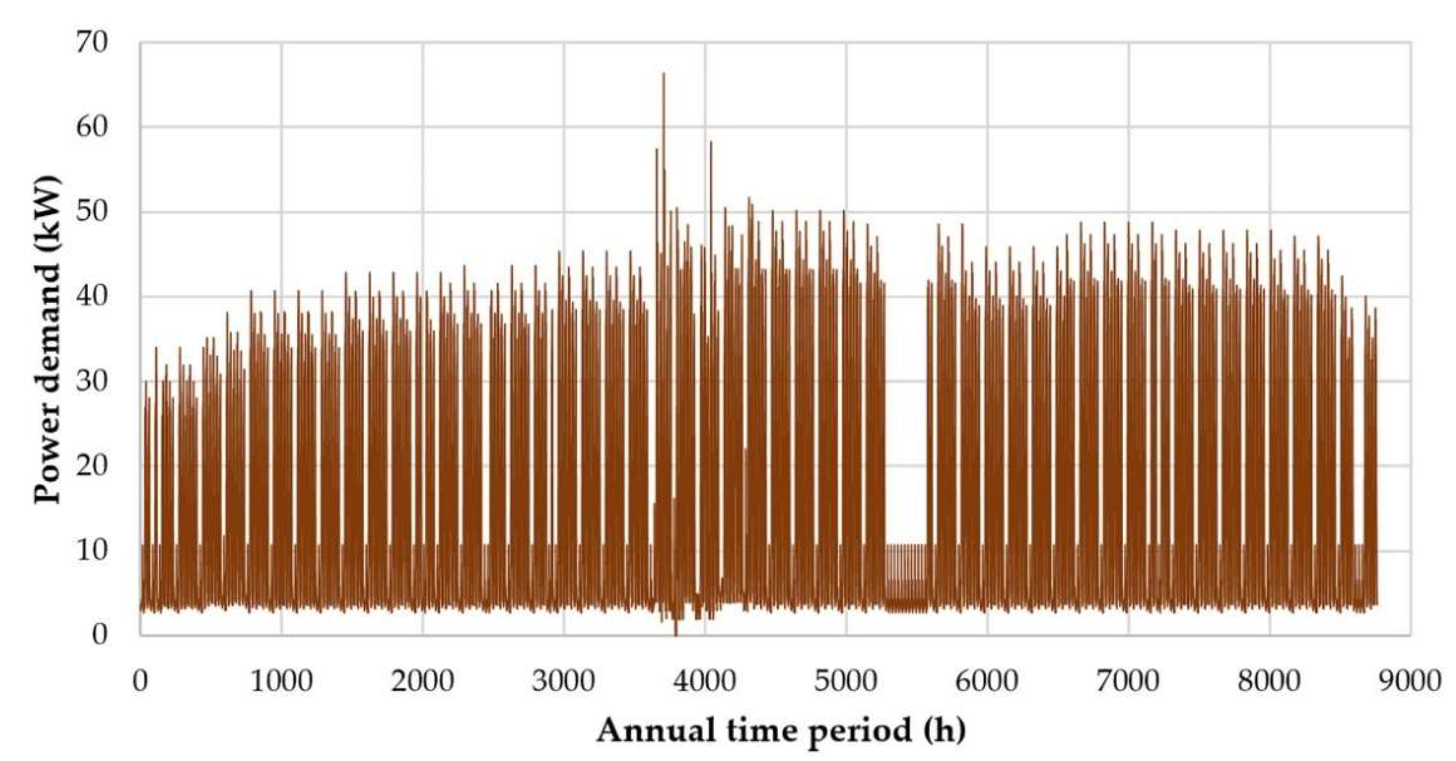
Figure 6.
Power demand fluctuation in the aluminum frames manufacturing factory from the 29th of June to the 8th of July 2025.
Figure 6.
Power demand fluctuation in the aluminum frames manufacturing factory from the 29th of June to the 8th of July 2025.
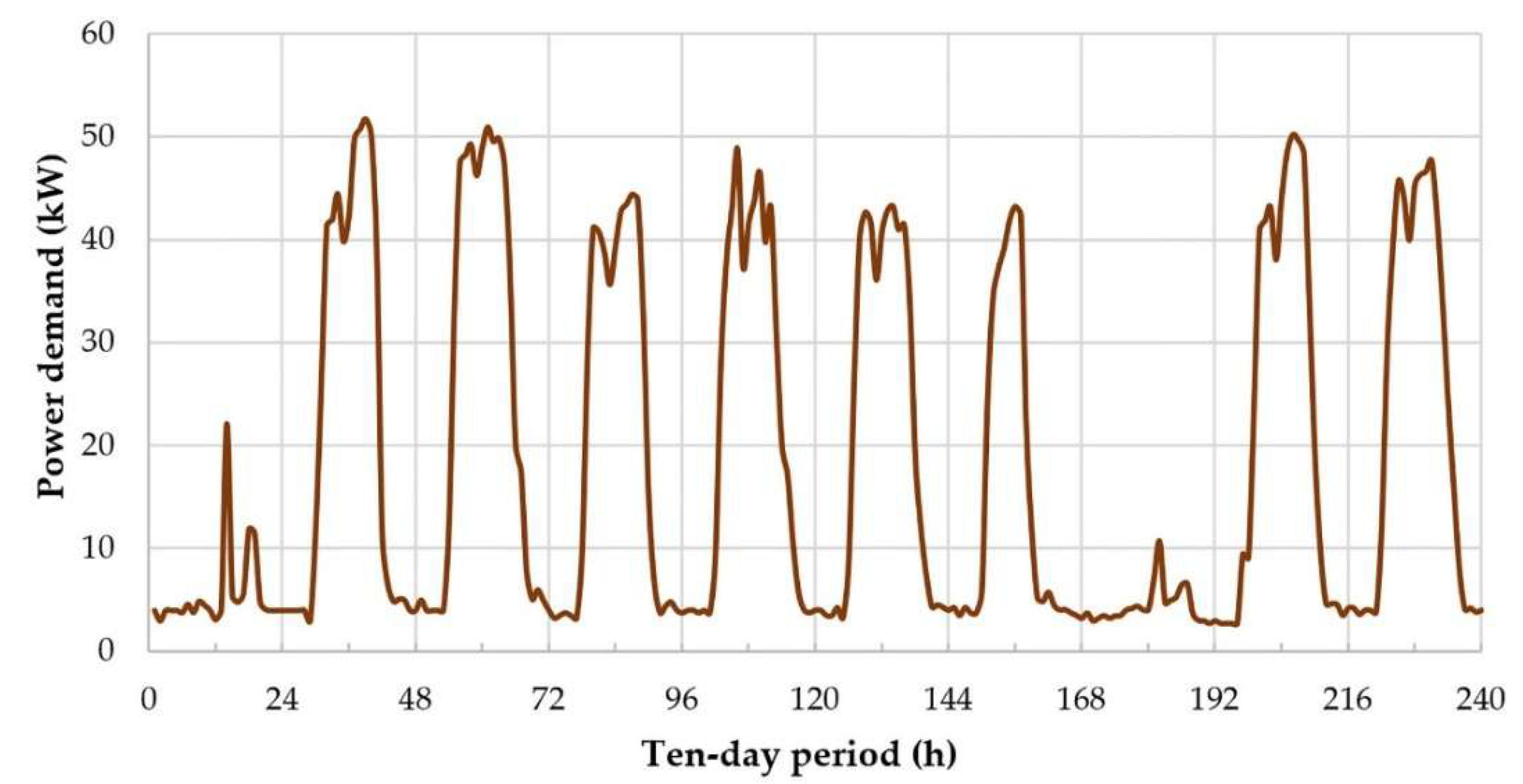
Figure 7.
Power demand daily measurements from 4 randomly selected residential consumers.
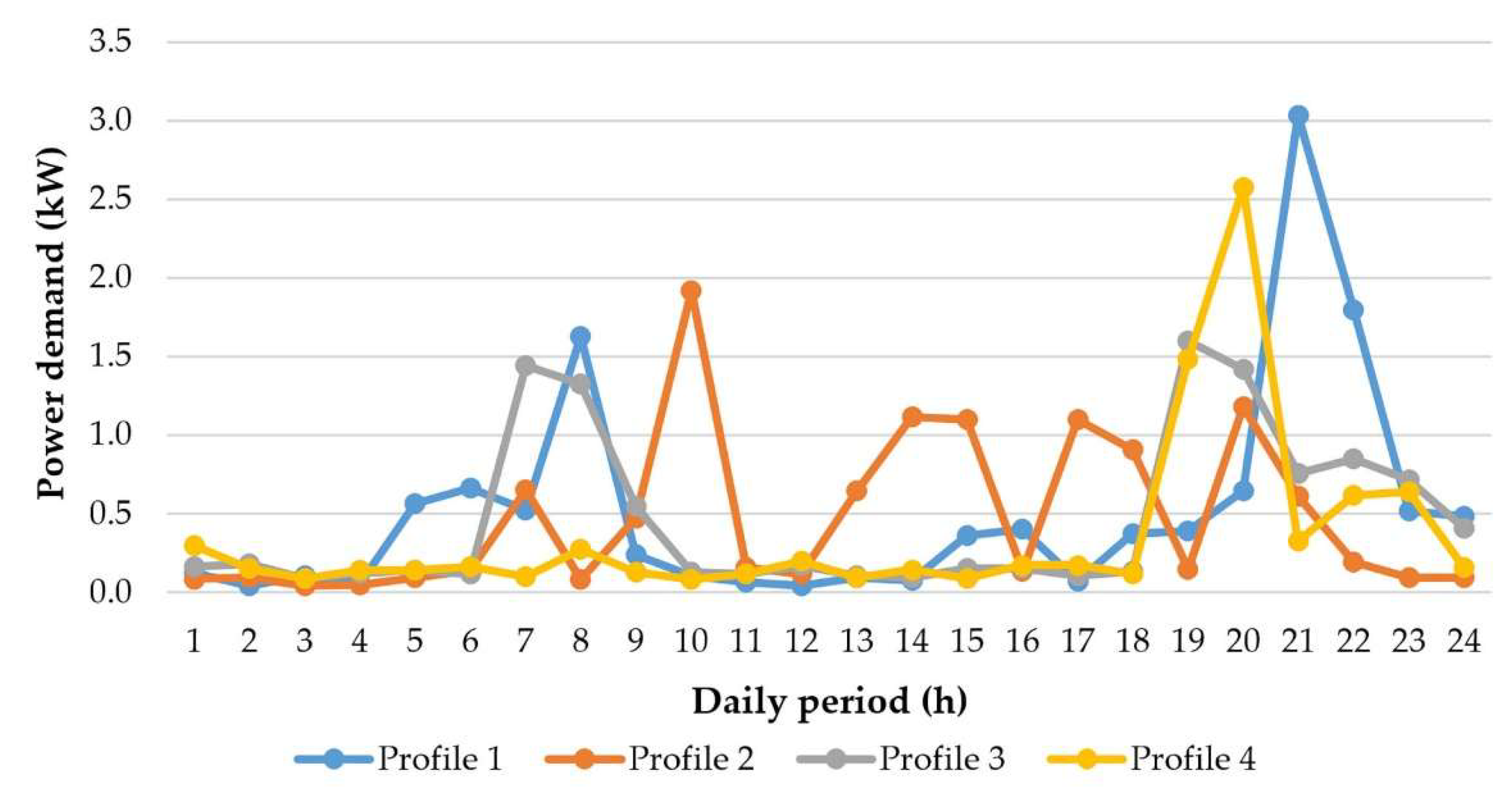
Figure 8.
Power demand daily measurements versus the number of children in the household.
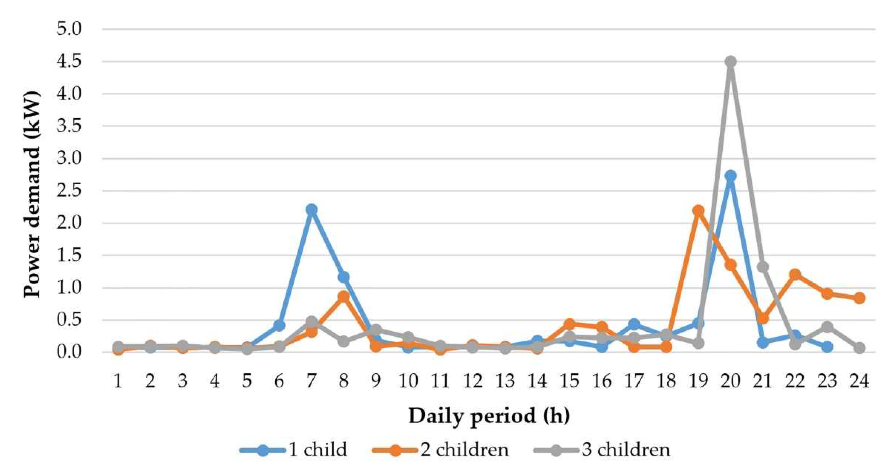
Figure 9.
Annual power demand fluctuation for a mixture of 100 residences.
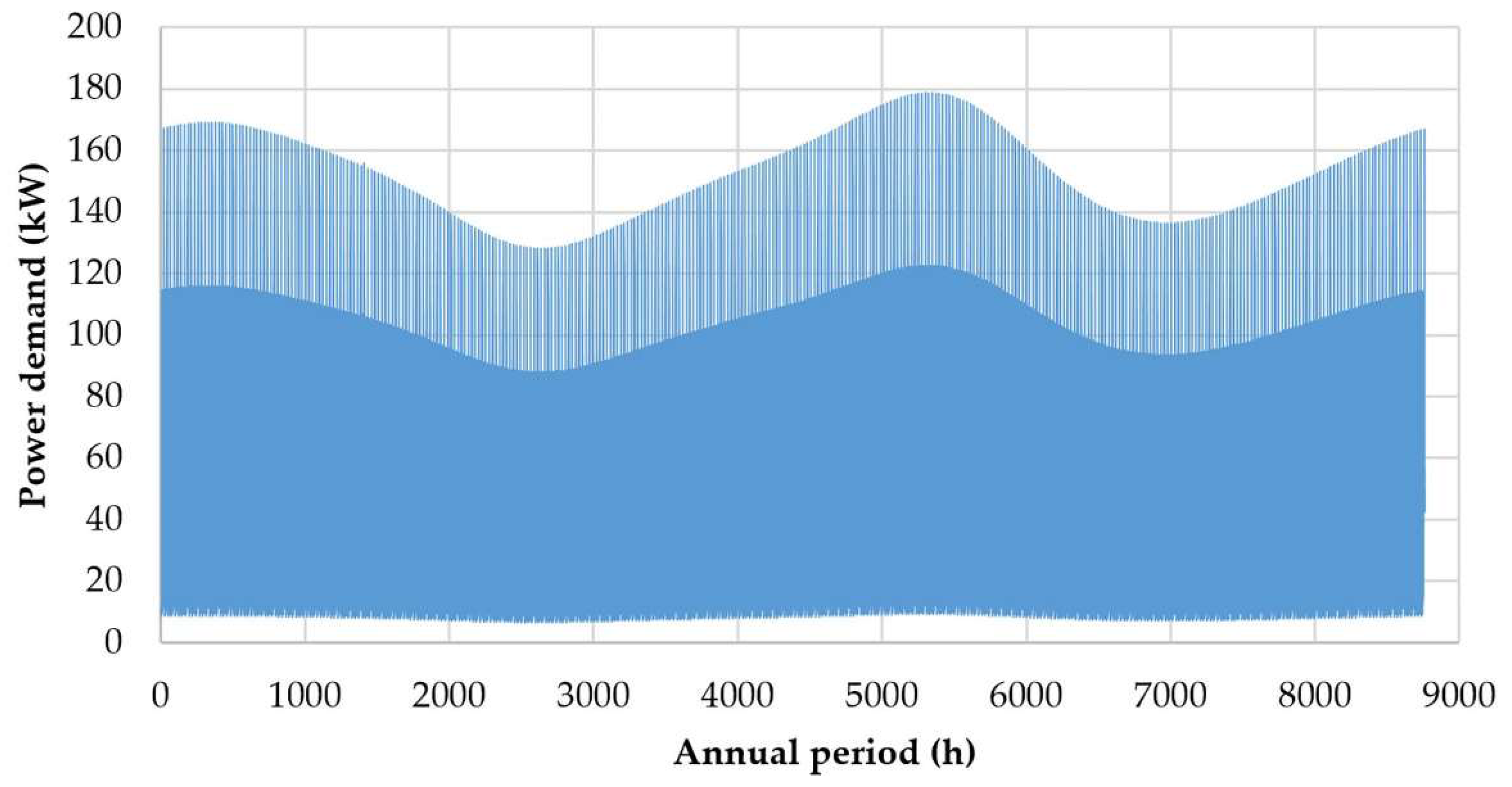
Figure 10.
Power demand fluctuation for a mixture of 100 residences from the 5th to the 14th of July.
Figure 10.
Power demand fluctuation for a mixture of 100 residences from the 5th to the 14th of July.
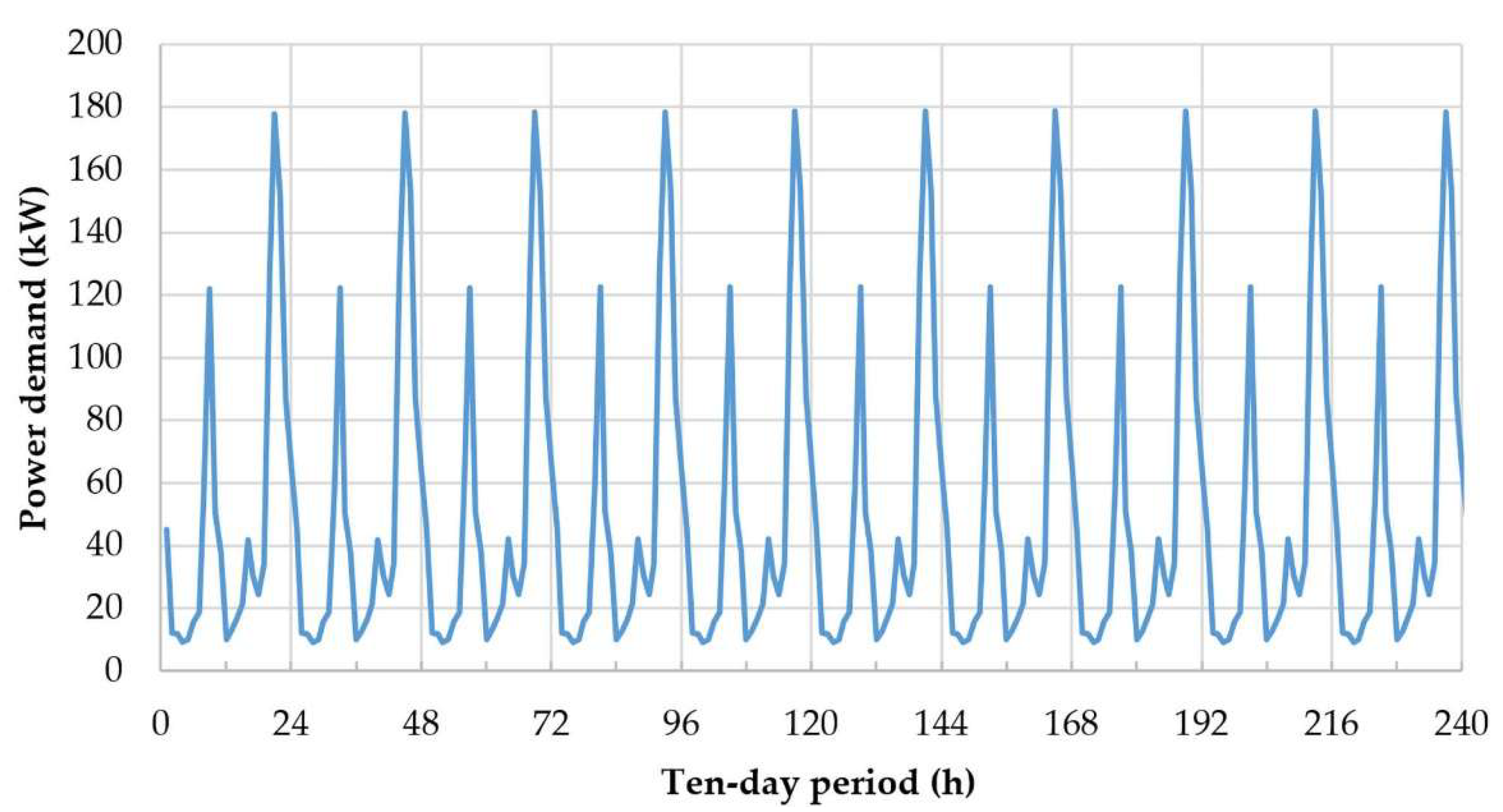
Figure 11.
Annual power demand fluctuation in the travel agency in 2025.
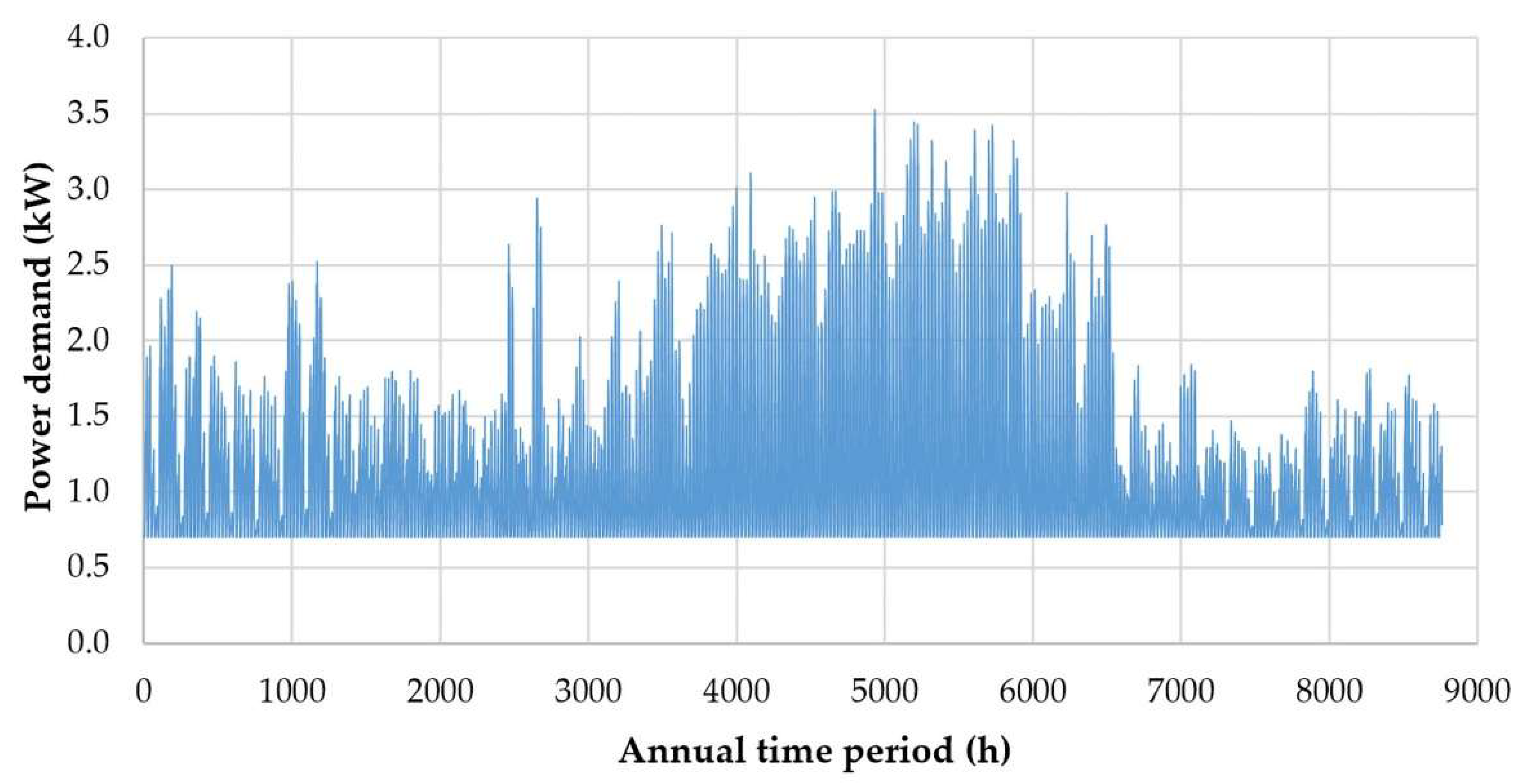
Figure 12.
Power demand fluctuation in the travel agency from the 1st to the 10th of August.
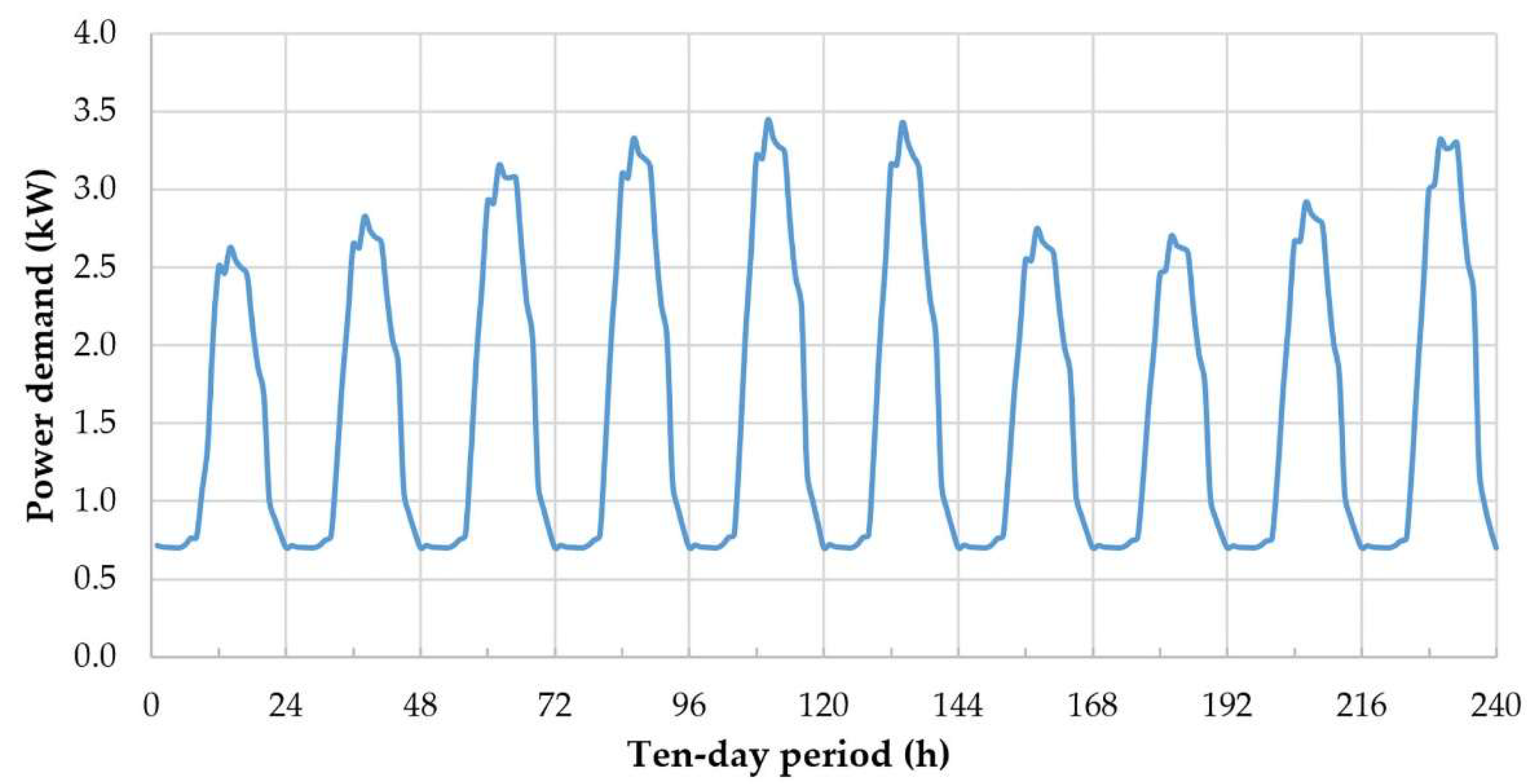
Figure 13.
Ambient temperature annual fluctuation.
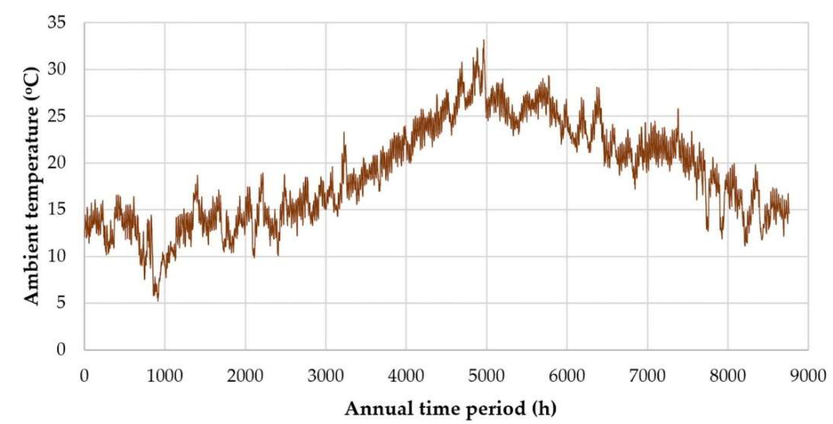
Figure 14.
Clear sky incident solar irradiance on horizontal plane.
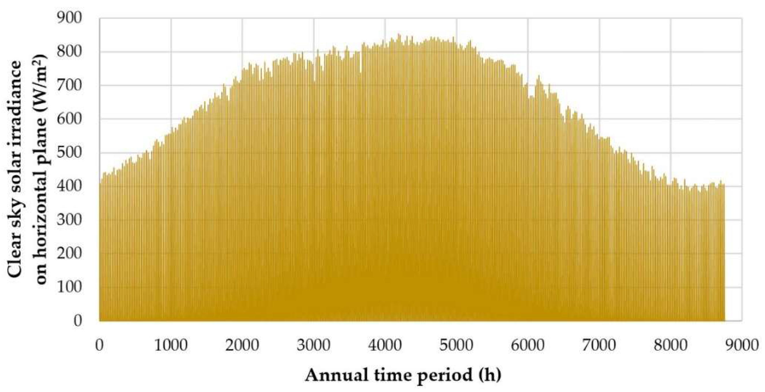
Figure 15.
Wind velocity annual fluctuation.
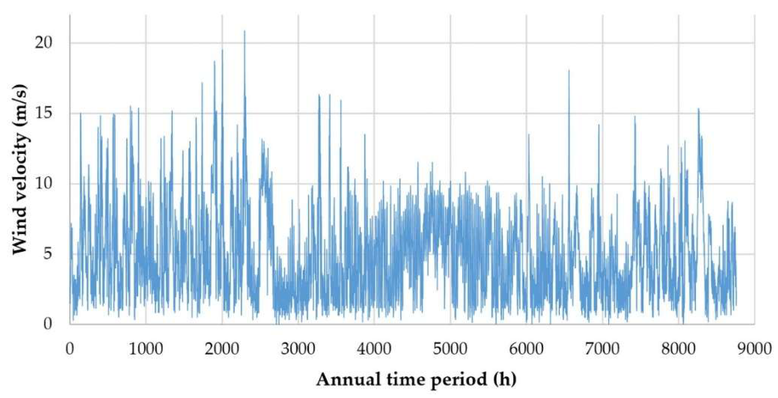
Figure 16.
Annual fluctuation of the incident solar irradiance on a south-facing surface tilted at 30° at the northern coastline of Prefecture of Heraklion in Crete.
Figure 16.
Annual fluctuation of the incident solar irradiance on a south-facing surface tilted at 30° at the northern coastline of Prefecture of Heraklion in Crete.
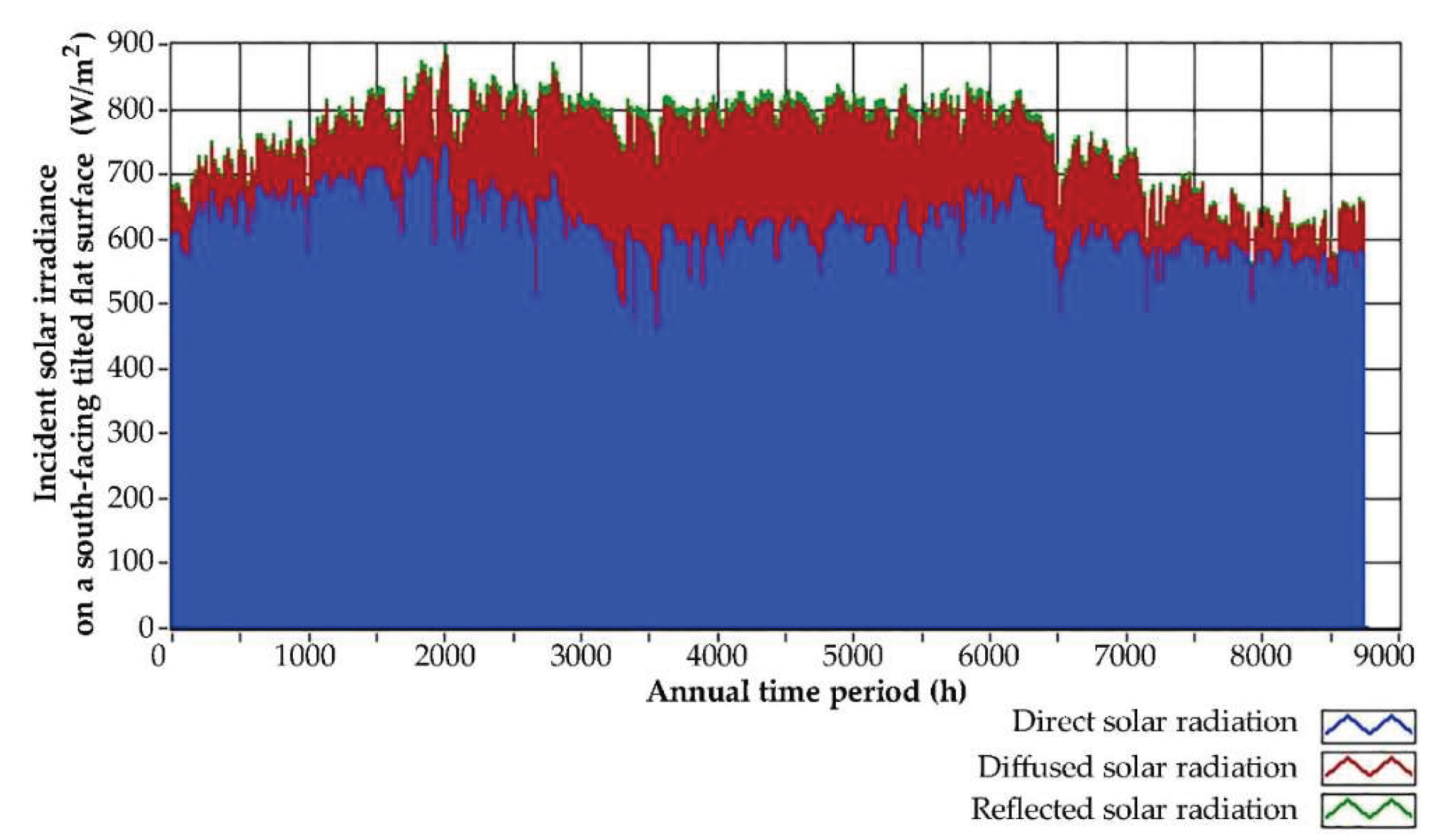
Figure 17.
Annual fluctuation of the photovoltaic power production per kWp of installed photovoltaic capacity.
Figure 17.
Annual fluctuation of the photovoltaic power production per kWp of installed photovoltaic capacity.
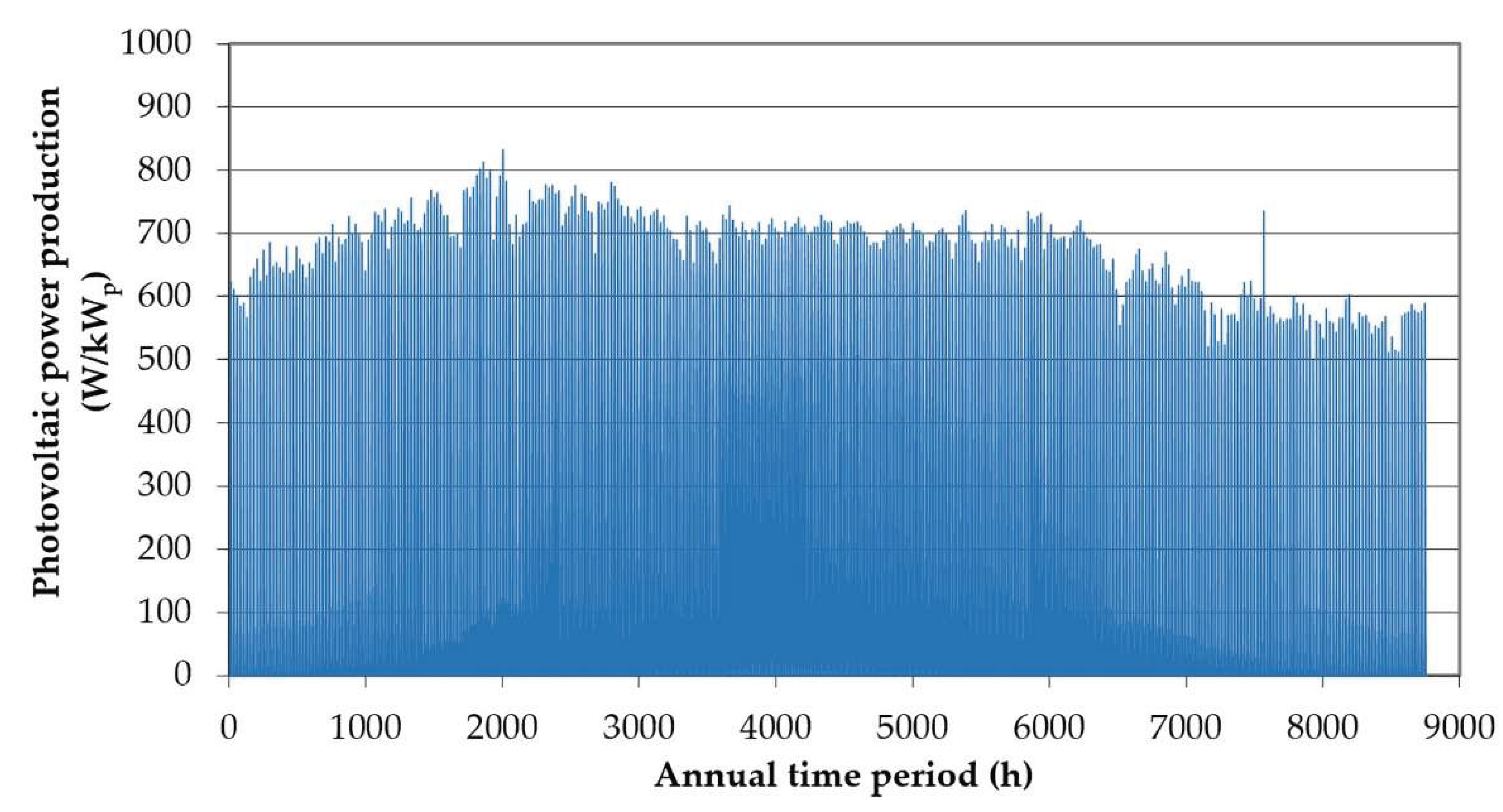
Figure 18.
Graphical depiction of the investigated scenarios’ results for the HMU main campus.
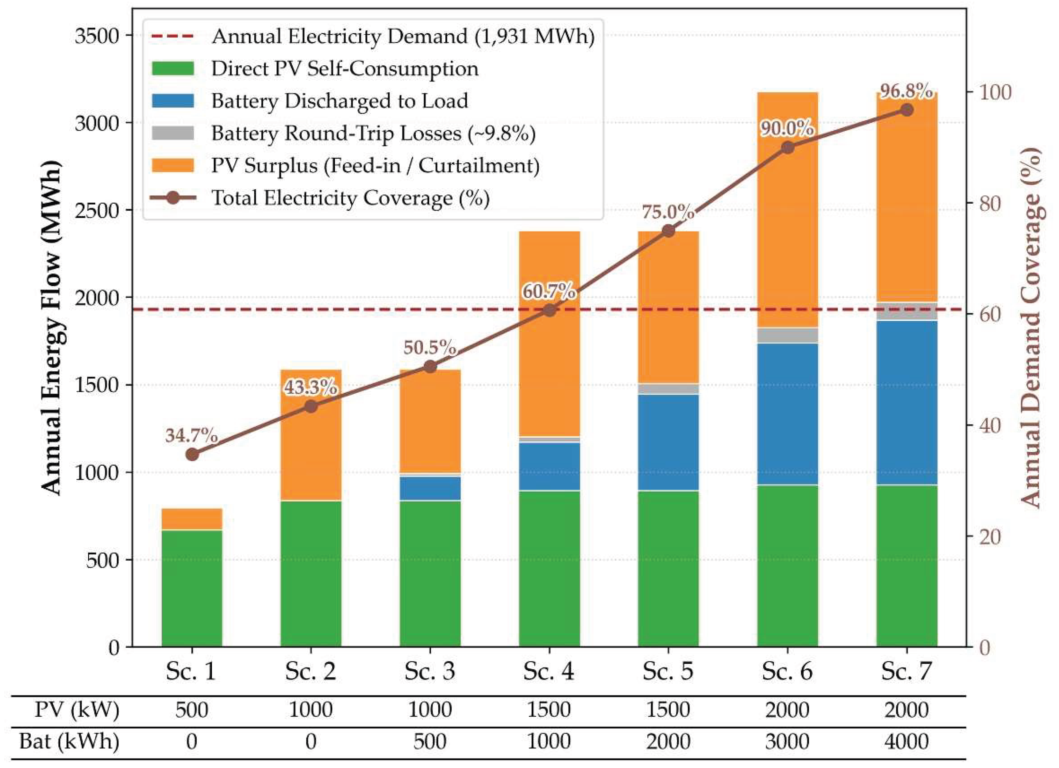
Figure 19.
Graphical depiction of the investigated scenarios’ results for the Crete Aquarium.
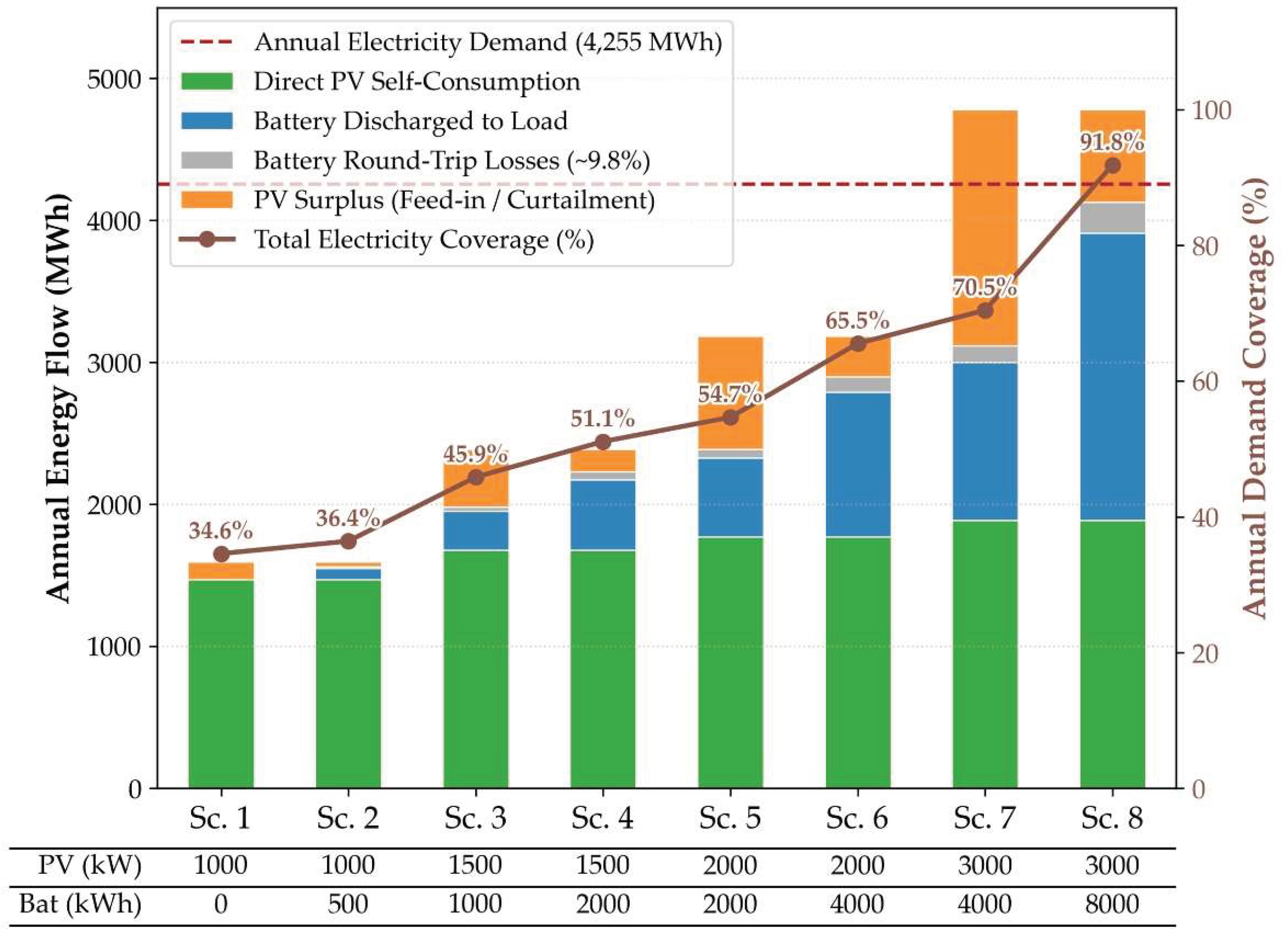
Figure 20.
Graphical depiction of the investigated scenarios’ results for the industrial facility.
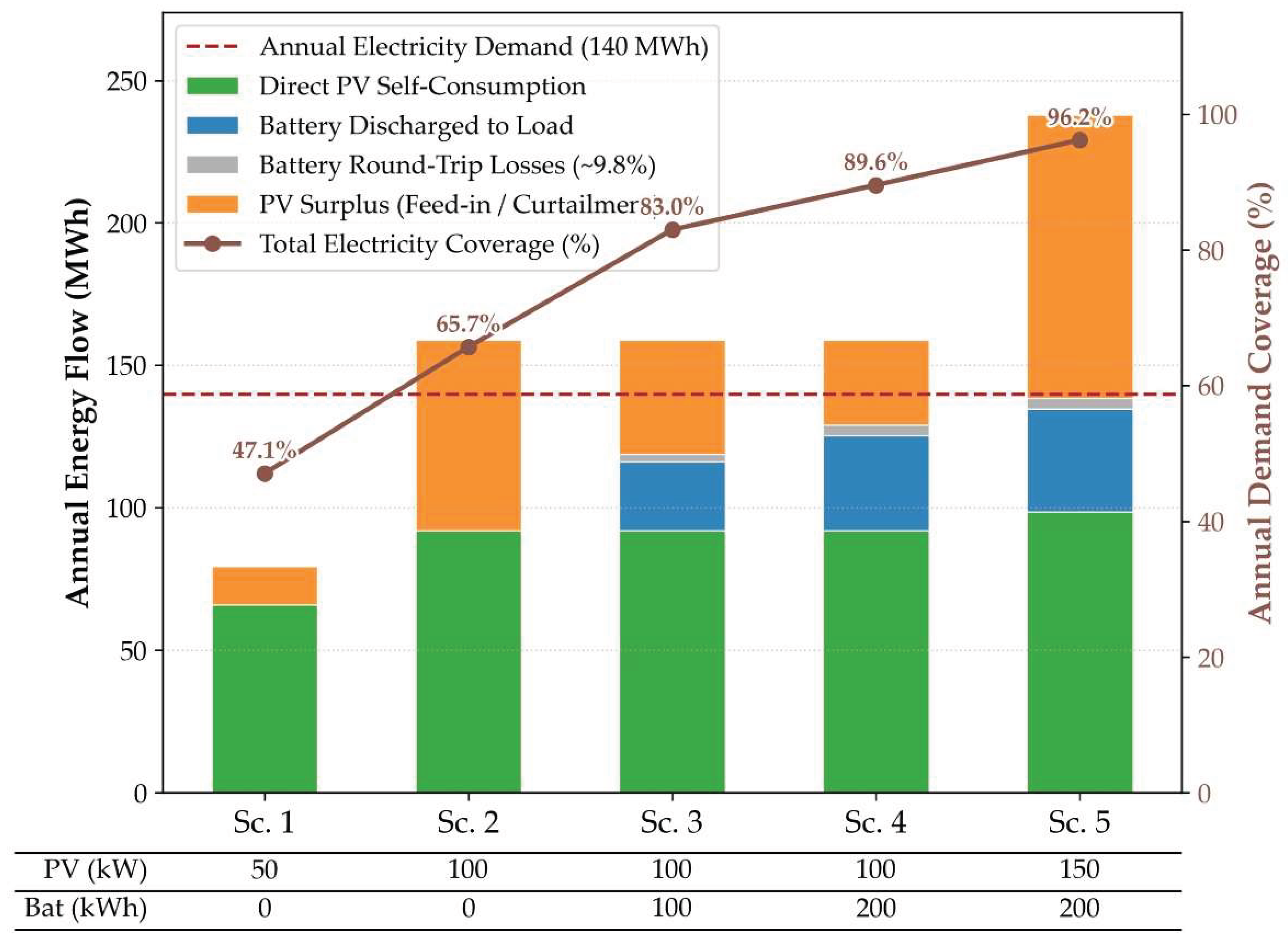
Figure 21.
Graphical depiction of the investigated scenarios’ results for the residential buildings.
Figure 21.
Graphical depiction of the investigated scenarios’ results for the residential buildings.
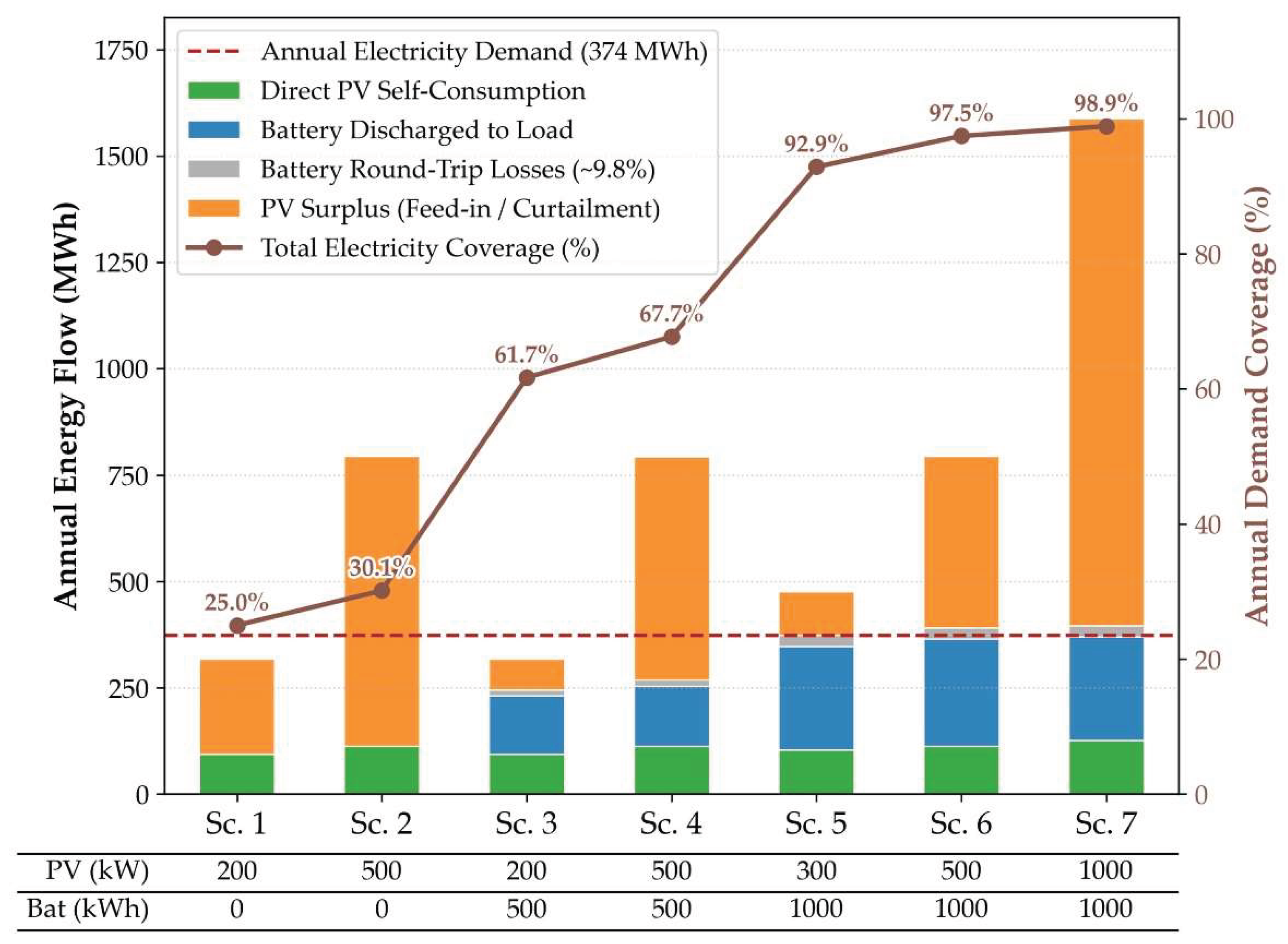
Figure 22.
Graphical depiction of the investigated scenarios’ results for the travel agency.
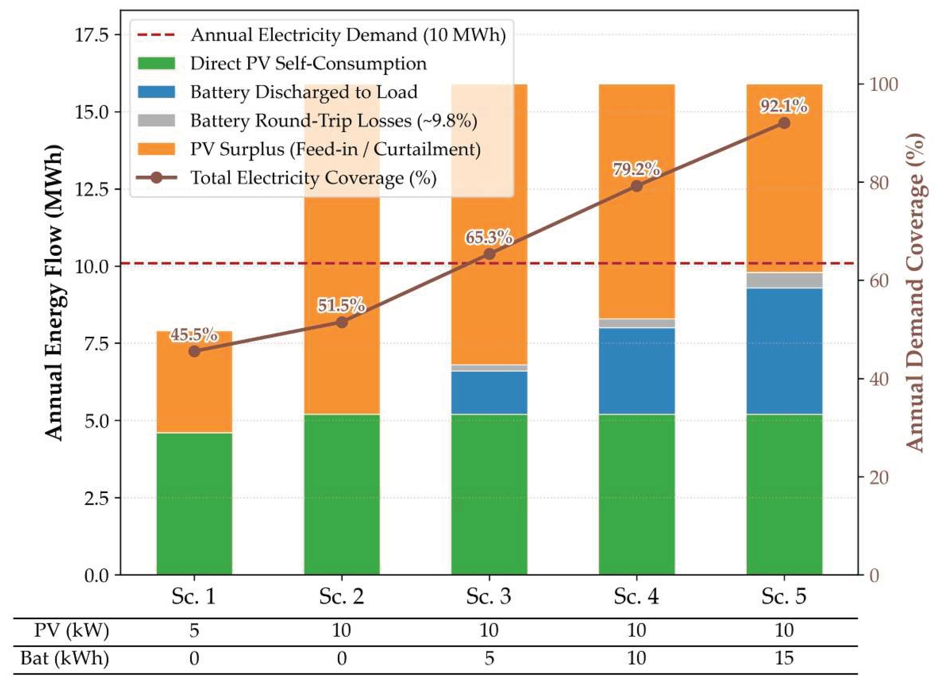

Table 1.
Synopsis of the available data on the electricity consumption and procurement cost of the investigated facilities.
Table 1.
Synopsis of the available data on the electricity consumption and procurement cost of the investigated facilities.
| Magnitude | HMU | Crete Aquarium | Aluminum frames factory |
Travel agency | 100 residences |
|---|---|---|---|---|---|
| Annual electricity consumption (kWh) | 1,930,979 | 4,134,743 | 140,323 | 10,165 | 373,920 |
| Annual peak power demand (kW) |
589.8 | 850.1 | 66.4 | 3.5 | 178.7 |
| Total annual procurement cost (EUR) |
487,327 | 898,089 | N/A | N/A | N/A |
| Total annual procurement specific cost (EUR/kWh) |
0.2524 | 0.2172 | N/A | N/A | N/A |
Table 2.
Variation of annually cumulative incident solar irradiation on a south-facing flat surface as a function of its tilt with regard to the horizontal plane.
Table 2.
Variation of annually cumulative incident solar irradiation on a south-facing flat surface as a function of its tilt with regard to the horizontal plane.
| Solar radiation component |
South-facing flat surface tilt with regard to the horizontal plane | ||||||
|---|---|---|---|---|---|---|---|
| 15ο | 20ο | 25ο | 30ο | 35ο | 40ο | 45ο | |
| Annually incident cumulative solar irradiation on flat inclined surface (kWh/m2) | |||||||
| Direct | 1038.9 | 1065.2 | 1083.4 | 1093.3 | 1095.0 | 1088.2 | 1073.3 |
| Diffused | 702.7 | 693.3 | 681.4 | 667.0 | 650.2 | 631.2 | 610.2 |
| Reflected | 7.4 | 13.1 | 20.4 | 29.1 | 39.3 | 50.9 | 63.7 |
| Total | 1749.0 | 1771.6 | 1785.1 | 1789.4 | 1784.5 | 1770.3 | 1747.1 |
Table 3.
Models and technologies of electrochemical batteries involved in the study.
| Required capacity (kWh) |
Commercially available model |
Nominal capacity (kWh) |
Number of units | Cost per unit (€) | Storage cycles | Lifespan (years) |
|---|---|---|---|---|---|---|
| 5 | Huawei LUNA2000–5-S0 / S1 (5 kWh) |
5 | 1 | 6000 | 6000 | 15 |
| 10 | BYD Battery-Box Premium HVS 10.2 | 10 | 1 | 9000 | 6000 | 15 |
| 15 | Fronius Battery Flex 16.7 | 16.7 | 1 | 12,500 | 6000 | 15 |
| 100 | BYD Battery-Max Lite (~100 kWh) |
100 | 1 | 55,000 | 7000 | 18 |
| 200 | BSLBATT ESS-GRID C225/C241 | 200 | 1 | 75,000 | 6000 | 15 |
| 500 | Sungrow PowerStack ST556kWh | 500 | 1 | 180,000 | 6000 | 15 |
| 1000 | BSL BATT ESS-GRID FlexiO series (500kW / 1MWh) |
1000 | 1 | 320,000 | 6000 | 15 |
| 2000 | Huawei LUNA2000- 2.0MWH-2H1 |
2000 | 1 | 580,000 | 6000 | 15 |
| 3000 | Capture Energy BESS PowerBox LC 1.6 MW / 3 MWh | 3000 | 1 | 900,000 | 6000 | 15 |
| 4000 | Huawei LUNA2000- 2.0MWH-2H1 |
2000 | 2 | 580,000 | 6000 | 15 |
| 8000 | Envision Energy – EN 8 Pro (8 MWh) & Gen 8 Platform | 8000 | 1 | 1,900,000 | 16,000 | 25 |
Table 4.
Summary table of simulation results for the alternative sizing scenarios regarding the photovoltaic plant and the battery storage system for the case of the HMU main campus.
Table 4.
Summary table of simulation results for the alternative sizing scenarios regarding the photovoltaic plant and the battery storage system for the case of the HMU main campus.
| Magnitude | Investigated scenario | ||||||
|---|---|---|---|---|---|---|---|
| 1 | 2 | 3 | 4 | 5 | 6 | 7 | |
| Essential sizing figures | |||||||
| Photovoltaic nominal power (kW) | 500 | 1000 | 1000 | 1500 | 1500 | 2000 | 2000 |
| Batteries storage capacity (kWh) | 0 | 0 | 500 | 1000 | 2000 | 3000 | 4000 |
| Energy results | |||||||
| Initial photovoltaic annual production (MWh) | 793.8 | 1587.7 | 1587.7 | 2381.5 | 2381.5 | 3175.3 | 3175.3 |
| Annual electricity coverage from PVs (MWh) | 669.6 | 837.0 | 837.0 | 893.4 | 893.4 | 927.3 | 927.3 |
| Annual electricity coverage from the batteries (MWh) | 0.0 | 0.0 | 138.8 | 277.9 | 554.0 | 811.1 | 941.8 |
| Total annual electricity coverage (MWh) | 669.6 | 837.0 | 975.8 | 1171.3 | 1447.4 | 1738.3 | 1869.1 |
| Total annual electricity coverage percentage (%) | 34.7 | 43.3 | 50.5 | 60.7 | 75.0 | 90.0 | 96.8 |
| Annual electricity storage from PVs (MWh) | 0.0 | 0.0 | 153.6 | 307.6 | 613.6 | 899.0 | 1044.4 |
| Total electricity absorbed from PVs (MWh) | 669.6 | 837.0 | 990.6 | 1201.0 | 1507.0 | 1826.3 | 1971.7 |
| Annual PVs electricity surplus percentage (%) | 15.7 | 47.3 | 37.6 | 49.6 | 36.7 | 42.5 | 37.9 |
| Economic results | |||||||
| Photovoltaic plant set-up cost (€∙103) | 400.0 | 800.0 | 800.0 | 1200.0 | 1200.0 | 1600.0 | 1600.0 |
| Batteries cost (€∙103) | 0.0 | 0.0 | 180.0 | 320.0 | 580.0 | 900.0 | 1100.0 |
| Total cost (€∙103) | 400.0 | 800.0 | 980.0 | 1520.0 | 1780.0 | 2500.0 | 2700.0 |
| Lifespan (years) | 25 | 25 | 15 | 15 | 15 | 15 | 15 |
| Electricity procurement cost annual drop (€∙103) | 169.0 | 211.3 | 246.3 | 295.6 | 365.3 | 438.8 | 471.8 |
| Payback period (years) | 2.4 | 3.8 | 4.0 | 5.1 | 4.9 | 5.7 | 5.7 |
| Electricity coverage specific cost (€/kWh) | 0.0239 | 0.0382 | 0.0670 | 0.0865 | 0.0820 | 0.0959 | 0.0963 |
Table 5.
Summary table of simulation results for the alternative sizing scenarios regarding the photovoltaic plant and the battery storage system for the case of the Crete Aquarium.
Table 5.
Summary table of simulation results for the alternative sizing scenarios regarding the photovoltaic plant and the battery storage system for the case of the Crete Aquarium.
| Magnitude | Investigated scenario | |||||||
|---|---|---|---|---|---|---|---|---|
| 1 | 2 | 3 | 4 | 5 | 6 | 7 | 8 | |
| Essential sizing figures | ||||||||
| Photovoltaic nominal power (kW) | 1000 | 1000 | 1500 | 1500 | 2000 | 2000 | 3000 | 3000 |
| Batteries storage capacity (kWh) | 0 | 500 | 1000 | 2000 | 2000 | 4000 | 4000 | 8000 |
| Energy results | ||||||||
| Initial photovoltaic annual production (MWh) | 1592.2 | 1592.2 | 2388.2 | 2388.2 | 3184.3 | 3184.3 | 4776.5 | 4776.5 |
| Annual electricity coverage from PVs (MWh) | 1471.0 | 1471.0 | 1675.1 | 1675.1 | 1771.5 | 1771.5 | 1887.0 | 1887.0 |
| Annual electricity coverage from the batteries (MWh) | 0.0 | 78.5 | 276.0 | 498.8 | 554.7 | 1017.6 | 1110.7 | 2021.1 |
| Total annual electricity coverage (MWh) | 1471.0 | 1549.4 | 1951.2 | 2173.9 | 2326.1 | 2789.1 | 2997.7 | 3908.1 |
| Total annual electricity coverage percentage (%) | 34.6 | 36.4 | 45.9 | 51.1 | 54.7 | 65.5 | 70.4 | 91.8 |
| Annual electricity storage from PVs (MWh) | 0.0 | 86.8 | 305.5 | 552.0 | 613.9 | 1126.3 | 1229.5 | 2237.8 |
| Total electricity absorbed from PVs (MWh) | 1471.0 | 1557.7 | 1980.7 | 2227.2 | 2385.4 | 2897.7 | 3116.5 | 4124.7 |
| Annual PVs electricity surplus percentage (%) | 7.6 | 2.2 | 17.1 | 6.7 | 25.1 | 9.0 | 34.8 | 13.6 |
| Economic results | ||||||||
| Photovoltaic plant set-up cost (€∙103) | 800.0 | 800.0 | 1200.0 | 1200.0 | 1600.0 | 1600.0 | 2400.0 | 2400.0 |
| Batteries cost (€∙103) | 0.0 | 180.0 | 320.0 | 580.0 | 580.0 | 1100.0 | 1100.0 | 1900.0 |
| Total cost (€∙103) | 800.0 | 980.0 | 1520.0 | 1780.0 | 2180.0 | 2700.0 | 3500.0 | 4300.0 |
| Lifespan (years) | 25 | 15 | 15 | 15 | 15 | 15 | 15 | 25 |
| Electricity procurement cost annual drop (€∙103) | 319.5 | 336.5 | 423.8 | 472.2 | 505.2 | 605.8 | 651.1 | 848.8 |
| Payback period (years) | 2.5 | 2.9 | 3.6 | 3.8 | 4.3 | 4.5 | 5.4 | 5.1 |
| Electricity coverage specific cost (€/kWh) | 0.0218 | 0.0422 | 0.0519 | 0.0546 | 0.0625 | 0.0645 | 0.0778 | 0.0440 |
Table 6.
Summary table of simulation results for the alternative sizing scenarios regarding the photovoltaic plant and the battery storage system for the case of the industrial facility.
Table 6.
Summary table of simulation results for the alternative sizing scenarios regarding the photovoltaic plant and the battery storage system for the case of the industrial facility.
| Magnitude | Investigated scenario | ||||
|---|---|---|---|---|---|
| 1 | 2 | 3 | 4 | 5 | |
| Essential sizing figures | |||||
| Photovoltaic nominal power (kW) | 50 | 100 | 100 | 100 | 150 |
| Batteries storage capacity (kWh) | 0 | 0 | 100 | 200 | 200 |
| Energy results | |||||
| Initial photovoltaic annual production (MWh) | 79.4 | 158.8 | 158.8 | 158.8 | 238.1 |
| Annual electricity coverage from PVs (MWh) | 65.9 | 92.0 | 92.0 | 92.0 | 98.6 |
| Annual electricity coverage from the batteries (MWh) | 0.0 | 0.0 | 24.2 | 33.4 | 36.1 |
| Total annual electricity coverage (MWh) | 65.9 | 92.0 | 116.2 | 125.4 | 134.7 |
| Total annual electricity coverage percentage (%) | 47.0 | 65.6 | 82.8 | 89.4 | 96.0 |
| Annual electricity storage from PVs (MWh) | 0.0 | 0.0 | 26.8 | 37.0 | 39.9 |
| Total electricity absorbed from PVs (MWh) | 65.9 | 92.0 | 118.8 | 129.0 | 138.6 |
| Annual PVs electricity surplus percentage (%) | 16.9 | 42.0 | 25.2 | 18.8 | 41.8 |
| Economic results | |||||
| Photovoltaic plant set-up cost (€∙103) | 40.0 | 80.0 | 80.0 | 80.0 | 120.0 |
| Batteries cost (€∙103) | 0 | 0.0 | 55.0 | 75.0 | 75.0 |
| Total cost (€∙103) | 40.0 | 80.0 | 135.0 | 155.0 | 195.0 |
| Lifespan (years) | 25 | 25 | 15 | 15 | 15 |
| Electricity procurement cost annual drop (€∙103) | 14.3 | 20.0 | 25.2 | 27.2 | 29.3 |
| Payback period (years) | 2.8 | 4.0 | 5.3 | 5.7 | 6.7 |
| Electricity coverage specific cost (€/kWh) | 0.0243 | 0.0348 | 0.0774 | 0.0824 | 0.0965 |
Table 7.
Summary table of simulation results for the alternative sizing scenarios regarding the photovoltaic plant and the battery storage system for the case of the residential consumers.
Table 7.
Summary table of simulation results for the alternative sizing scenarios regarding the photovoltaic plant and the battery storage system for the case of the residential consumers.
| Magnitude | Investigated scenario | ||||||
|---|---|---|---|---|---|---|---|
| 1 | 2 | 3 | 4 | 5 | 6 | 7 | |
| Essential sizing figures | |||||||
| Photovoltaic nominal power (kW) | 200 | 500 | 200 | 500 | 300 | 500 | 1000 |
| Batteries storage capacity (kWh) | 0 | 0 | 500 | 500 | 1000 | 1000 | 1000 |
| Energy results | |||||||
| Initial photovoltaic annual production (MWh) | 317.5 | 793.9 | 317.5 | 793.9 | 476.3 | 793.9 | 1587.7 |
| Annual electricity coverage from PVs (MWh) | 93.4 | 112.6 | 93.4 | 112.6 | 103.4 | 112.6 | 125.6 |
| Annual electricity coverage from the batteries (MWh) | 0.0 | 0.0 | 137.3 | 140.7 | 244.0 | 251.9 | 244.4 |
| Total annual electricity coverage (MWh) | 93.4 | 112.6 | 230.7 | 253.3 | 347.4 | 364.5 | 369.9 |
| Total annual electricity coverage percentage (%) | 25.0 | 30.1 | 61.7 | 67.7 | 92.9 | 97.5 | 98.9 |
| Annual electricity storage from PVs (MWh) | 0.0 | 0.0 | 151.9 | 155.7 | 270.1 | 278.9 | 270.6 |
| Total electricity absorbed from PVs (MWh) | 93.4 | 112.6 | 245.3 | 268.4 | 373.4 | 391.5 | 396.1 |
| Annual PVs electricity surplus percentage (%) | 70.6 | 85.8 | 22.7 | 66.2 | 21.6 | 50.7 | 75.1 |
| Economic results | |||||||
| Photovoltaic plant set-up cost (€∙103) | 160.0 | 400.0 | 160.0 | 400.0 | 240.0 | 400.0 | 800.0 |
| Batteries cost (€∙103) | 0.0 | 0.0 | 180.0 | 180.0 | 320.0 | 320.0 | 320.0 |
| Total cost (€∙103) | 160.0 | 400.0 | 340.0 | 580.0 | 560.0 | 720.0 | 1120.0 |
| Lifespan (years) | 25 | 25 | 15 | 15 | 15 | 15 | 15 |
| Electricity procurement cost annual drop (€∙103) | 20.3 | 24.5 | 50.1 | 55.0 | 75.4 | 77.5 | 80.3 |
| Payback period (years) | 7.9 | 16.4 | 6.8 | 10.5 | 7.4 | 9.3 | 13.9 |
| Electricity coverage specific cost (€/kWh) | 0.0685 | 0.1421 | 0.0983 | 0.1526 | 0.1075 | 0.1345 | 0.2018 |
Table 8.
Summary table of simulation results for the alternative sizing scenarios regarding the photovoltaic plant and the battery storage system for the case of the commercial facility.
Table 8.
Summary table of simulation results for the alternative sizing scenarios regarding the photovoltaic plant and the battery storage system for the case of the commercial facility.
| Magnitude | Investigated scenario | ||||||
|---|---|---|---|---|---|---|---|
| 1 | 2 | 3 | 4 | 5 | |||
| Essential sizing figures | |||||||
| Photovoltaic nominal power (kW) | 5 | 10 | 10 | 10 | 10 | ||
| Batteries storage capacity (kWh) | 0 | 0 | 5 | 10 | 15 | ||
| Energy results | |||||||
| Initial photovoltaic annual production (MWh) | 7.9 | 15.9 | 15.9 | 15.9 | 15.9 | ||
| Annual electricity coverage from PVs (MWh) | 4.6 | 5.2 | 5.2 | 5.2 | 5.2 | ||
| Annual electricity coverage from the batteries (MWh) | 0.0 | 0.0 | 1.4 | 2.8 | 4.1 | ||
| Total annual electricity coverage (MWh) | 4.6 | 5.2 | 6.6 | 8.0 | 9.3 | ||
| Total annual electricity coverage percentage (%) | 45.4 | 51.4 | 65.2 | 78.9 | 91.9 | ||
| Annual electricity storage from PVs (MWh) | 0.0 | 0.0 | 1.6 | 3.1 | 4.6 | ||
| Total electricity absorbed from PVs (MWh) | 4.6 | 5.2 | 6.8 | 8.3 | 9.8 | ||
| Annual PVs electricity surplus percentage (%) | 41.9 | 67.1 | 57.3 | 47.6 | 38.4 | ||
| Economic results | |||||||
| Photovoltaic plant set-up cost (€∙103) | 4.0 | 8.0 | 8.0 | 8.0 | 8.0 | ||
| Batteries cost (€∙103) | 0.0 | 0.0 | 6.0 | 9.0 | 12.5 | ||
| Total cost (€∙103) | 4.0 | 8.0 | 14.0 | 17.0 | 20.5 | ||
| Lifespan (years) | 25 | 25 | 15 | 15 | 15 | ||
| Electricity procurement cost annual drop (€∙103) | 1.0 | 1.1 | 1.4 | 1.7 | 2.0 | ||
| Payback period (years) | 4.0 | 7.1 | 9.7 | 9.8 | 10.1 | ||
| Electricity coverage specific cost (€/kWh) | 0.0347 | 0.0613 | 0.1408 | 0.1413 | 0.1463 | ||
Disclaimer/Publisher’s Note: The statements, opinions and data contained in all publications are solely those of the individual author(s) and contributor(s) and not of MDPI and/or the editor(s). MDPI and/or the editor(s) disclaim responsibility for any injury to people or property resulting from any ideas, methods, instructions or products referred to in the content. |
© 2026 by the authors. Licensee MDPI, Basel, Switzerland. This article is an open access article distributed under the terms and conditions of the Creative Commons Attribution (CC BY) license (http://creativecommons.org/licenses/by/4.0/).
Copyright: This open access article is published under a Creative Commons CC BY 4.0 license, which permit the free download, distribution, and reuse, provided that the author and preprint are cited in any reuse.