
Submitted:
30 September 2026
Posted:
30 September 2026
You are already at the latest version
Abstract
Lithological mapping is essential for geological exploration, though fieldwork-based mapping is often limited by time, cost, and accessibility. This study proposes an integrated methodology to support lithological mapping of the Coastal Batholith between San Gregorio and Chepén, using Landsat 8, ASTER, and Sentinel-2 imagery, DEM-derived morphometric variables, and the Random Forest algorithm, applying dimensionality reduction techniques (PCA, MNF, ICA) and field-based validation. Results showed robust performance across all three sensors, with Landsat 8 achieving the highest accuracy (Overall Accuracy = 76.1 %, Kappa = 0.736, F1-score = 76.8 %), followed by Sentinel-2 (OA = 75.3 %) and ASTER (OA = 73.0 %). Morphometric variables, particularly elevation, contributed 44–48 % of the model's total importance, proving key for identifying Quaternary de-posits. Field verification confirmed the reliability of the resulting mapping, demonstrating that integrating multisensor data, morphometric variables, and Random Forest is an effective method-ology for geological exploration.
Keywords:
lithological mapping
; remote sensing
; machine learning
; random forest
; morphometric variables
; coastal batholith
1. Introduction
Lithological mapping constitutes an essential tool for geological characterization and mineral resource exploration. In recent years, satellite remote sensing and machine learning have demonstrated significant potential to complement traditional mapping methods, enabling the efficient analysis of large areas. In this context, the present study proposes the integration of Landsat 8, ASTER, and Sentinel-2 imagery, morphometric variables derived from DEMs, statistical techniques, and Machine Learning algorithms to support lithological mapping of the Coastal Batholith in the area between San Gregorio and Chepén. The objective is to evaluate the potential of these tools to improve the discrimination of lithological units and optimize geological exploration activities.
2. Study Area
2.1. Location and Accessibility
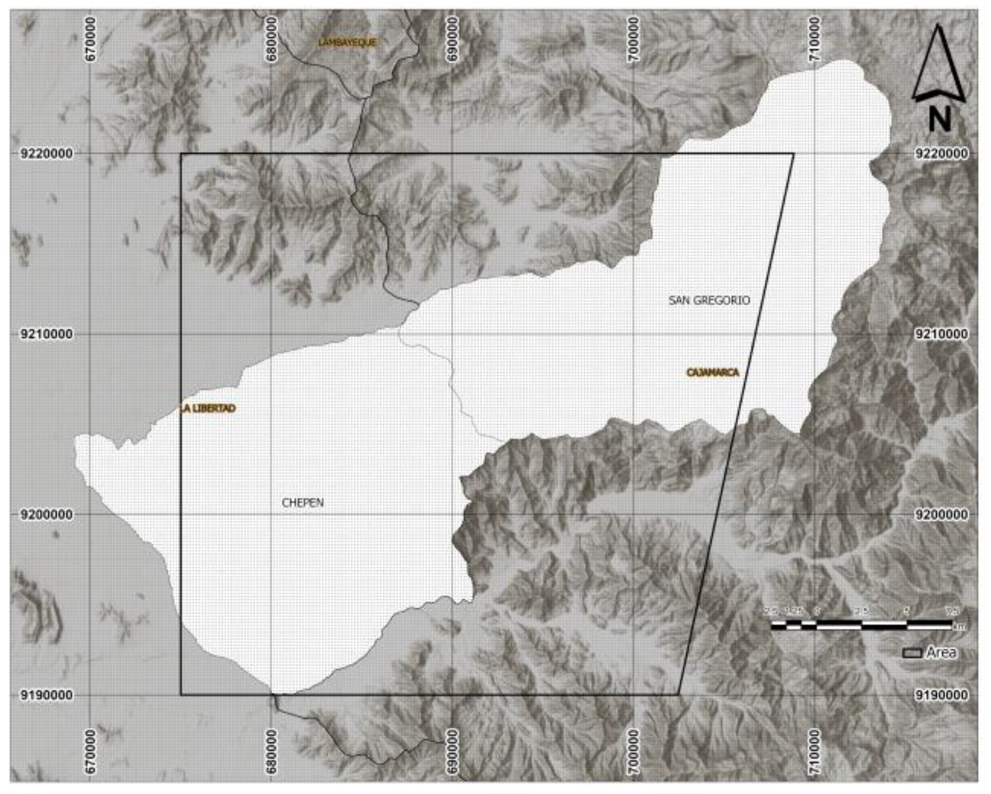
The study area is located between San Gregorio and Chepén, in northern Peru, within the Coastal Batholith, and covers an approximate area of 920.12 km².
Figure 1.
Location Map.
2.2.1. Regional Geology
The Coastal Batholith is composed of magmatic systems distributed along its emplacement, exhibiting characteristics that record partial melting of both the mantle and the crust [1]. Three main segments (Piura, Lima, and Arequipa) and two transitional zones (Chaparra–Caravelí and Trujillo–Chiclayo) have been proposed based on previous studies [1,2,3].
The study area is located within the Trujillo–Chiclayo transitional zone. This zone comprises several superunits whose composition ranges from gabbro to granite, following an intrusive sequence from basic to acidic compositions. These superunits are Patap, Paltashaco, Las Lomas, Noque, Santa Rosa, and Lagartos.
2.2.2. Local Geology
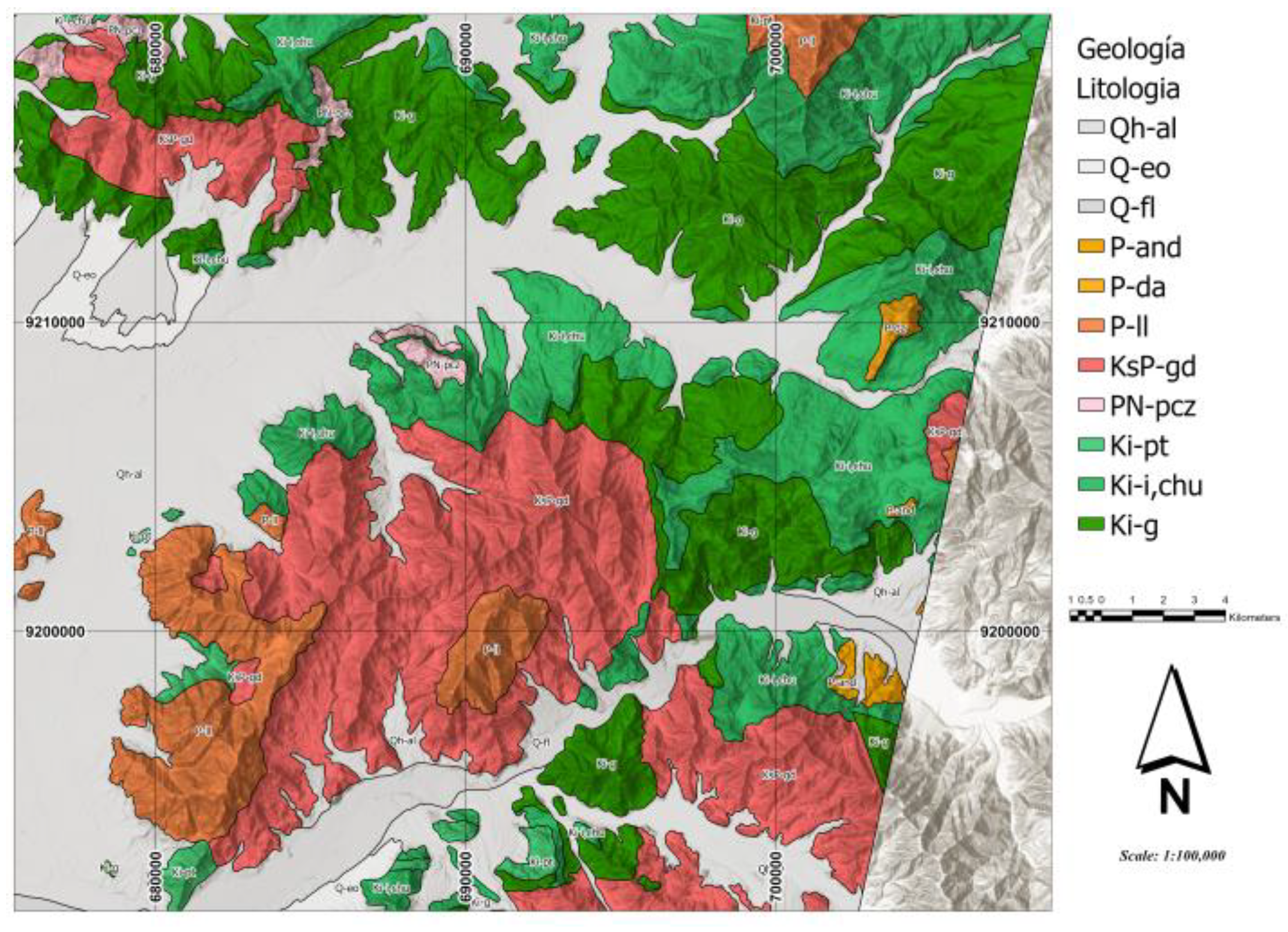
The study area comprises Mesozoic, Cenozoic, and Quaternary geological units. These include the Goyllarisquizga Group, composed of sandstones and limestones of Mesozoic age; the Inca Formation, consisting of calcareous sandstones; the Pariatambo Formation, characterized by bituminous limestones; and the Lagarto Formation, composed of ferruginous sandstones. The Calipuy Group represents a Cenozoic volcanic arc, comprising volcanic sequences ranging from the Eocene to the Miocene, in addition to Quaternary deposits consisting of dunes and alluvial sediments [4,5].
Figure 2.
Local geological map of the study area between San Gregorio and Chepén, showing the identified Mesozoic, Cenozoic, and Quaternary lithological units at a scale of 1:100,000.
Figure 2.
Local geological map of the study area between San Gregorio and Chepén, showing the identified Mesozoic, Cenozoic, and Quaternary lithological units at a scale of 1:100,000.
3. Materials and Methods
3.1. Data Used
3.1.1. Satellite Images
3.1.1.1. Landsat 8
The images from this satellite originate from its two onboard instruments: the Operational Land Imager (OLI) and the Thermal Infrared Sensor (TIRS). The OLI sensor provides access to nine spectral bands covering the spectrum from 0.433 µm to 1.390 µm, while TIRS records from 10.30 µm to 12.50 µm. They feature a 12-bit radiometric resolution and incorporate two new bands compared to previous versions: Band 1 (designed for water resources and coastal zone detection) and Band 9 (used for cirrus cloud detection). It provides moderate-resolution images ranging from 15 m per pixel for the panchromatic band to 100 m for the long-wave infrared [6].
3.1.1.2. ASTER
This satellite features 14 spectral bands, capturing data from the near-infrared, short-wave infrared, and thermal infrared regions, which aids in mineral identification due to their distinct spectral features. It includes three subsystems: VNIR, with 3 bands in the visible and near-infrared at a 15 m spatial resolution; SWIR, with 6 bands in the short-wave infrared at 30 m; and TIR, with 5 bands in the thermal infrared at a 90 m resolution [7].
3.1.1.3. Sentinel-2
This satellite provides high-resolution, wide-swath multispectral images. Its MultiSpectral Instrument (MSI) samples 13 spectral bands: visible and NIR at 10 meters, red edge and SWIR at 20 meters, and atmospheric bands at 60 meters of spatial resolution. Notably, its SWIR bands allow for the discrimination of clay minerals, iron oxides, and rock types with contrasting spectral characteristics [7].

Table 1.
Satellite images used in the study.
| Image Type | Cloud Cover | Acquisition Year | Platform |
|---|---|---|---|
| LANDSAT 8 | 10% | 2022 | USGS |
| ASTER | 10% | 2003 | EarthData |
| SENTINEL-2 | 10% | 2022 | Copernicus |
3.1.2. Digital Elevation Model
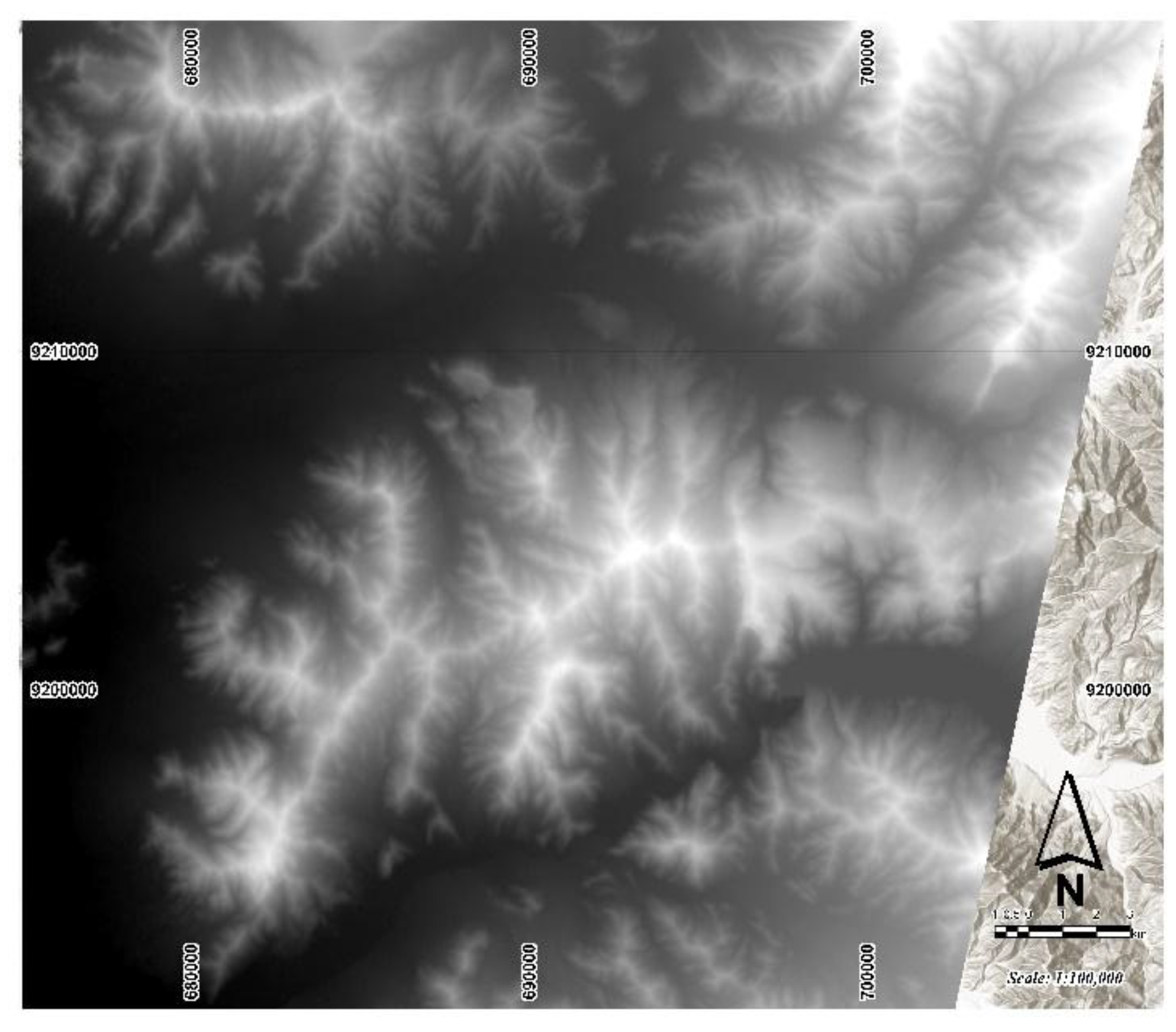
ALOS PALSAR is an L-band synthetic aperture radar system developed by JAXA, capable of acquiring information on the Earth's surface regardless of cloud cover and lighting conditions. Its 23.6 cm wavelength provides high penetration capacity through vegetation [8]. In this research, the ALOS PALSAR-derived DEM from 2018 was used to calculate the morphometric variables described below.
Figure 3.
Digital Elevation Model (DEM) of the study area.
3.2. Methods
3.2.1. Statistical Methods (Definitions of PCA, MNF, ICA)
Principal Component Analysis (PCA) is a mathematical technique that transforms datasets by creating new axes that are linear combinations of the original ones. These axes are orthogonal and uncorrelated with each other. The first component captures most of the total variance, and this variance decreases in subsequent components [9].
The Minimum Noise Fraction (MNF) transformation determines the dimensionality of an image, separates noise from the data, and reduces hardware requirements. It also analyzes spatial coherence in the eigenimages and helps identify the most informative bands for future analyses [10].
Independent Component Analysis (ICA) is a blind source separation technique that decomposes multiband data into statistically independent components. It maximizes statistical independence, which improves the separation of spectral signals in multispectral images, facilitating the identification of specific materials [11].
3.2.2. Morphometric Analysis
Geomorphometry is defined as the set of quantitative variables derived from the Digital Elevation Model that describe relief: elevation, slope, aspect, surface roughness (SR), hypsometric index (HI), and surface index (SI). These variables, calculated using moving windows over the DEM, allow for the quantification of topography and explain the control of relief over the lithological distribution in the study area [12].
3.2.3. Machine Learning Models (Random Forest)
This is an image classification algorithm used in remote sensing due to its internal accuracy estimation through cross-validation. This supervised machine learning algorithm consists of an ensemble of decision trees that employ bagging and feature randomness techniques to generate uncorrelated trees, thereby improving prediction accuracy. Its performance is determined using standard metrics such as overall accuracy and the Kappa coefficient [11].
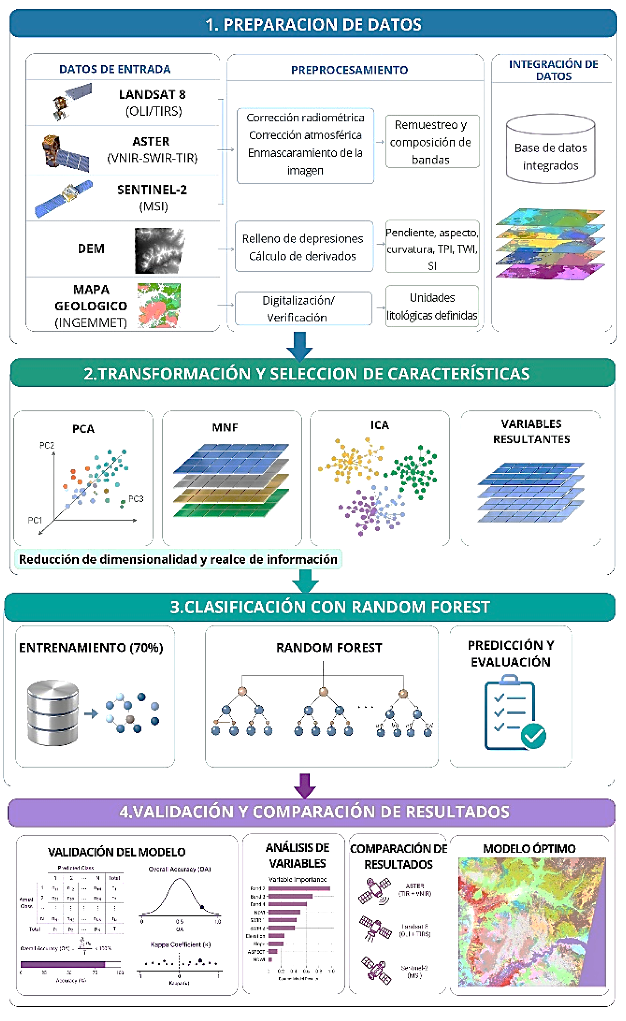
3.3. Methodology
Figure 4.
Methodological flowchart: data preparation, feature transformation, Random Forest classification, and validation.
Figure 4.
Methodological flowchart: data preparation, feature transformation, Random Forest classification, and validation.
4. Results and Discussion
4.1. Lithological Discrimination Using Spectral Transformations
4.1.1. Landsat 8
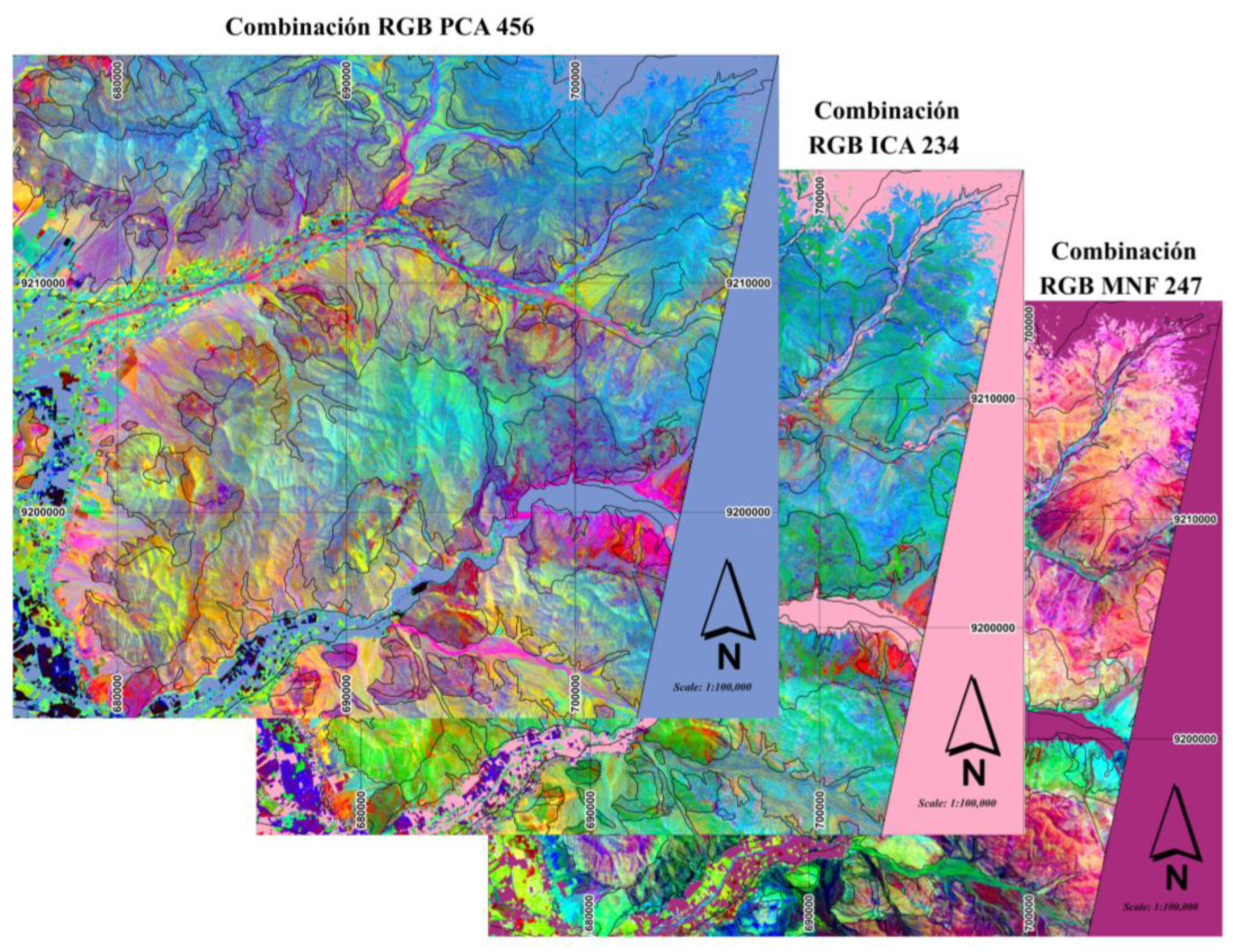
The PCA, MNF, and ICA transformations applied to the Landsat 8 images successfully highlighted the main lithological units present in the study area. However, the RGB PC4–PC5–PC6 composition derived from PCA showed the best performance for lithological discrimination, demonstrating the highest correspondence with the reference geological mapping and a clear differentiation among intrusive, volcanic, and carbonate rocks. This capability is supported by the high loading values of the selected components, where PC4 was dominated by bands B4 (+0.6302) and B5 (-0.4713), PC5 by B7 (+0.6061) and B6 (-0.6773), and PC6 by B3 (+0.7404) and B4 (-0.5295), highlighting zones with iron oxides and carbonate units, respectively. Meanwhile, the RGB MNF2–MNF4–MNF7 and RGB ICA2–ICA3–ICA4 compositions provided complementary information for geological interpretation. Consequently, all three transformations were incorporated as predictor variables in the Random Forest model.
Figure 5.
RGB compositions of the PCA, MNF, and ICA transformations applied to Landsat 8.
4.1.2. Sentinel-2
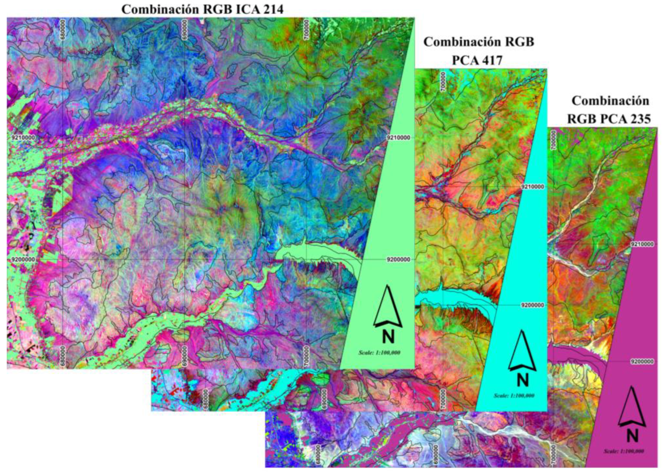
Sentinel-2A images, processed using PCA, MNF, and ICA transformations, improved the spectral contrast among the main lithological units of the San Gregorio and Chepén sector. Among the evaluated compositions, RGB ICA2–ICA1–ICA4 showed the best performance for lithological discrimination. This result is supported by the loading values of the selected components, where ICA2 was dominated by B3 (+0.8240), which is sensitive to carbonates and surface oxides; ICA1 by B2 (+0.9787), associated with the general reflectance of intrusive bodies; and ICA4 by the contrast between B5 (+0.7843) and B4 (−0.6161), which favored the differentiation between intrusive and volcanic units. Furthermore, the RGB PC4–PC1–PC5 composition—defined by the contrast between B11 (+0.549) and B6 (−0.316) in PC4, the general albedo in PC1, and the contrast between B2 (−0.610) and B8A (+0.544) in PC5—along with the MNF5–MNF3–MNF2 composition, which reduced instrumental noise effects, provided complementary spectral information for geological interpretation. Consequently, the three transformations were incorporated as predictor variables in the Random Forest classification model.
Figure 6.
RGB compositions of the ICA, PCA, and MNF transformations applied to Sentinel-2.
4.1.3. ASTER
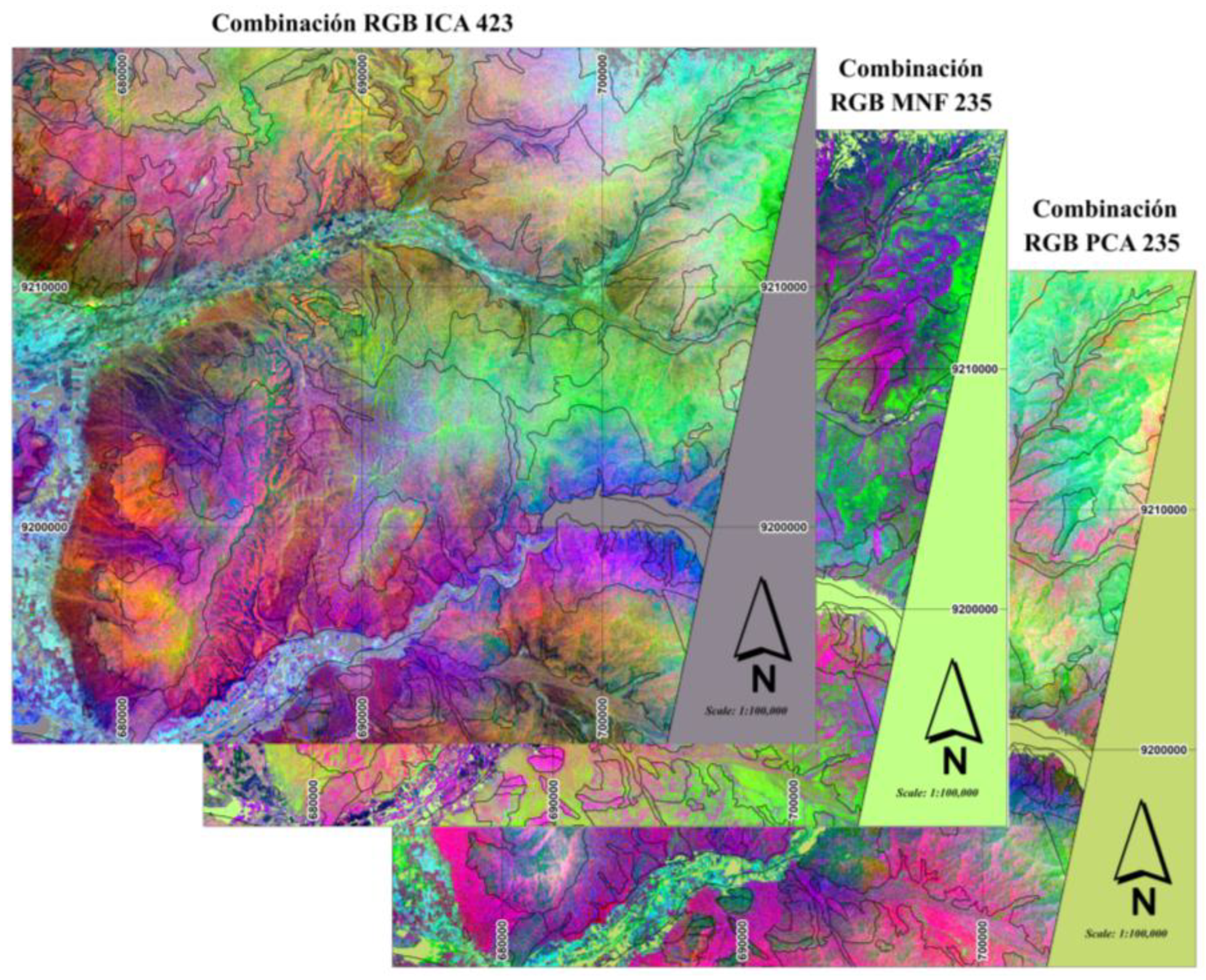
The processing of ASTER images using PCA, MNF, and ICA transformations improved the spectral differentiation of the main lithological units in the study area. Among the evaluated compositions, RGB ICA4–ICA2–ICA3 presented the best performance for lithological discrimination, displaying the highest correspondence with reference geological mapping and a clear differentiation among intrusive rocks, carbonates, and Quaternary deposits. This behavior is explained by the eigenvectors of the selected components, where ICA4 presented dominant loadings in SWIR-B5 (-0.621) and SWIR-B8 (+0.612), highlighting granodiorite bodies; ICA2, with a dominant loading in SWIR-B9 (+0.809) and SWIR-B4 (-0.453), allowed for the identification of Cretaceous carbonate formations and their argillic alteration halos; while ICA3, with a dominant loading in SWIR-B4 (+0.670), reinforced the spectral response of carbonates, favoring differentiation between intrusive and carbonate units. Meanwhile, the RGB PC2–PC3–PC5 and MNF2–MNF3–MNF5 compositions provided complementary information for geological interpretation, with the latter standing out for its superior visual quality due to the reduction of instrumental noise. Consequently, the three transformations were incorporated as predictor variables in the Random Forest classification model.
Figure 7.
RGB compositions of the ICA, PCA, and MNF transformations applied to the ASTER SWIR bands.
Figure 7.
RGB compositions of the ICA, PCA, and MNF transformations applied to the ASTER SWIR bands.
4.2. Random Forest Machine Learning Model Training
Table 2.
Data sources and input variables.
| Data Source | Transformation | Variables Used |
|---|---|---|
| Landsat 8 | PCA | PC4, PC5, PC6 |
| MNF | MNF2, MNF4, MNF7 | |
| ICA | ICA2, ICA3, ICA4 | |
| Sentinel-2 | PCA | PC4, PC1, PC5 (Note: adjusted from CP7 to match previous text/standard notation) |
| MNF | MNF5, MNF3, MNF2 | |
| ICA | ICA2, ICA1, ICA4 | |
| ASTER | PCA | PC2, PC3, PC5 |
| MNF | MNF2, MNF3, MNF5 | |
| ICA | ICA4, ICA2, ICA3 | |
| ALOS PALSAR Digital Elevation Model | Morphometry | Elevation |
| Slope | ||
| Aspect | ||
| Curvature | ||
| Profile Curvature | ||
| Planar Curvature | ||
| Topographic Position Index (TPI) | ||
| Terrain Ruggedness Index (TRI) |
4.3. Model Performance Evaluation
4.3.1. Classification Metrics
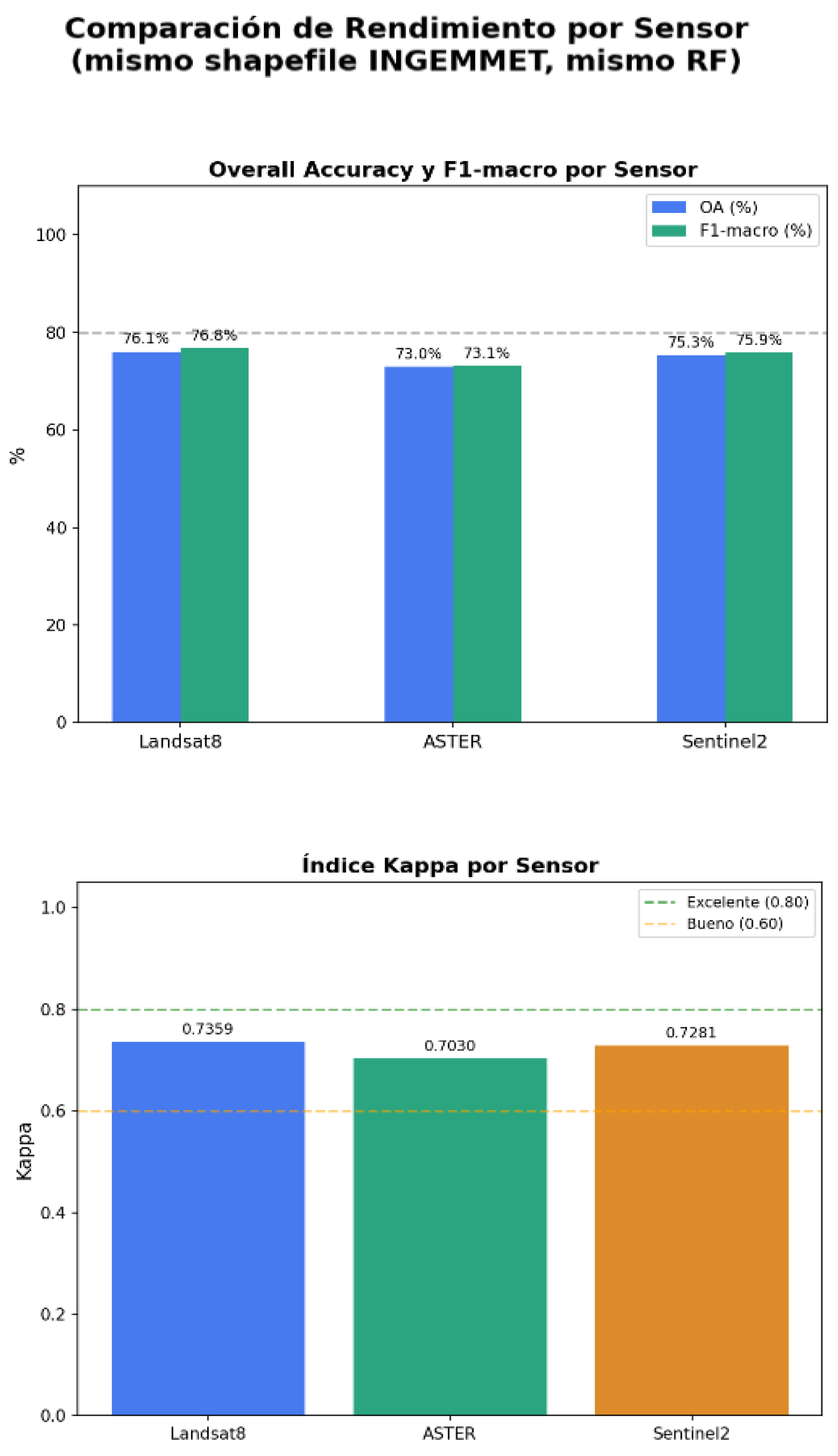
To evaluate the performance of the Random Forest models trained with Landsat 8, Sentinel-2, and ASTER images, Overall Accuracy (OA), Cohen's Kappa index, and the F1-score per class were used—metrics widely applied in supervised satellite image classification. The results show a solid and consistent performance across all three sensors, with Landsat 8 achieving the highest accuracy (OA = 76.1%, $\kappa$ = 0.736, and F1-score = 76.8%), followed by Sentinel-2 (OA = 75.3%, $\kappa$ = 0.728, and F1-score = 75.9%) and ASTER (OA = 73.0%, $\kappa$ = 0.703, and F1-score = 73.1%). According to the interpretation scale proposed by Landis and Koch [13], all obtained Kappa values correspond to substantial agreement (0.61–0.80), approaching the almost perfect agreement level ($\kappa$ > 0.80). Likewise, the minimal difference observed between OA and F1-score (< 1%) evidences an adequate balance among classes and a robust classification, allowing for a reliable comparison of each sensor's potential for lithological discrimination.
Figure 8.
Performance of the Random Forest models trained with Landsat 8, Sentinel-2, and ASTER images.
Figure 8.
Performance of the Random Forest models trained with Landsat 8, Sentinel-2, and ASTER images.
4.3.2. Performance by Lithological Unit
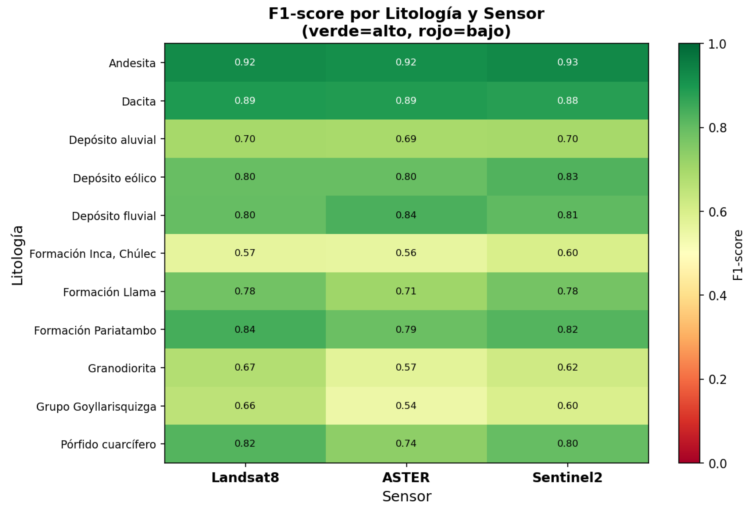
The analysis of the F1-score per lithological unit (Fig. 8) revealed a consistent pattern across the three sensors: extrusive volcanic units (Andesite and Dacite) achieved the highest values (F1 = 0.88–0.93), reflecting their high spectral and morphological separability relative to the rest of the lithologies. In contrast, units with greater geological affinity showed the lowest values: the Inca-Chúlec Formation (F1 = 0.56–0.60) and the Goyllarisquizga Group (F1 = 0.54–0.66), a result consistent with the confusion matrices (Fig. 9), where these two units concentrate the highest cross-confusion with each other (11–16% of the pixels of each class were erroneously assigned to the other). Granodiorite also exhibited intermediate performance (F1 = 0.57–0.67), with recurrent confusion toward the Pariatambo Formation and the Goyllarisquizga Group, possibly associated with hydrothermal alteration processes that modify their original spectral response. In comparative terms, Landsat 8 showed the most balanced performance among classes, whereas ASTER presented the largest F1 drop in units with similar lithofacies (Granodiorite = 0.57; Goyllarisquizga Group = 0.54), suggesting a lower capability of this sensor to discriminate units with subtle spectral signals in the used SWIR range.
Figure 9.
Comparative confusion matrix for Landsat 8, Sentinel-2, and ASTER images.
4.3.3. Importance of Predictor Variables
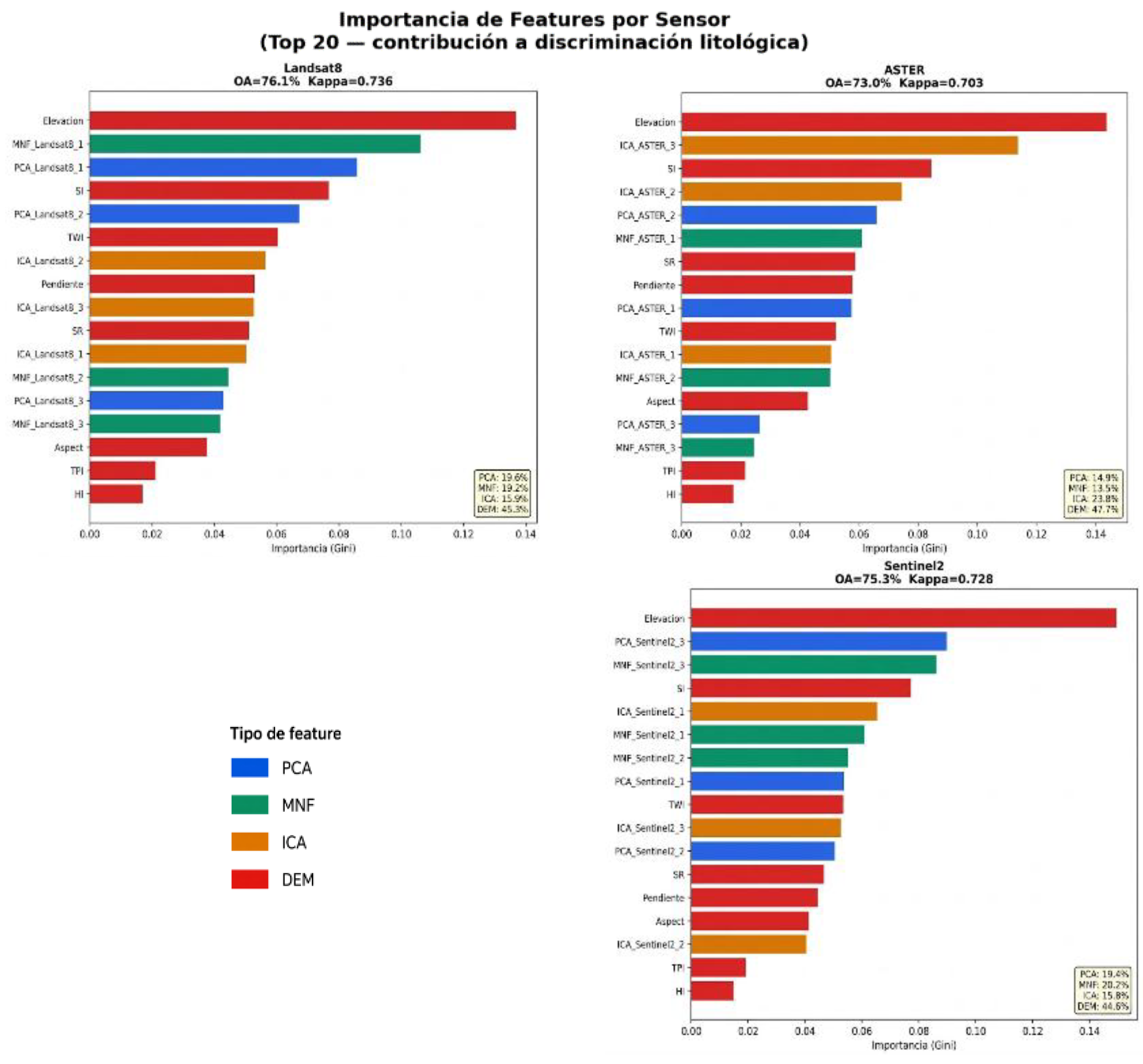
The variable importance analysis (Gini importance) of the Random Forest model showed a consistent pattern across the three sensors: morphometric variables derived from the DEM concentrated the highest relative contribution to the classification (44.6–47.7% of the total), with Elevation being the most important individual variable in all three cases, followed by the Surface Index (SI), Slope, and Topographic Wetness Index (TWI). This evidences that the topographic-morphological control associated with the differential resistance to erosion of each lithology constitutes a robust predictor independent of the optical sensor used. Among the spectral transformations, correspondence was observed with the described visual discrimination results: in ASTER, the ASTER ICA component was the second most important variable in the model (after Elevation), and the ICA set provided the highest relative contribution among spectral transformations (23.8%), consistent with its superior visual performance in this sensor. In Landsat 8, PCA and MNF showed practically equivalent contributions (19.6% and 19.2%, respectively), with Landsat 8 MNF-1 and Landsat 8 PCA as the most relevant spectral components, in line with the good visual performance reported for both transformations. In Sentinel-2, MNF and PCA also dominated over ICA in terms of cumulative contribution (20.2% and 19.4% versus 15.8%), although the ICA composition achieved the best visual discrimination; this apparent discrepancy suggests that while ICA visually highlights the most relevant lithological contrasts, the PCA and MNF components provide complementary information of greater cumulative statistical weight for the Random Forest model. Across all sensors, microscale morphometric variables (TPI, HI) exhibited the lowest relative importance, indicating that topographic-lithological control operates primarily at a regional scale (slope, elevation) rather than through micro-relief variations.
Figure 10.
Importance of predictor variables in the Random Forest models for Landsat 8, ASTER, and Sentinel-2.
Figure 10.
Importance of predictor variables in the Random Forest models for Landsat 8, ASTER, and Sentinel-2.
4.4. Validation and Interpretation of Lithological Mapping
4.4.1. Classification Results Obtained with Landsat 8, ASTER, and Sentinel-2
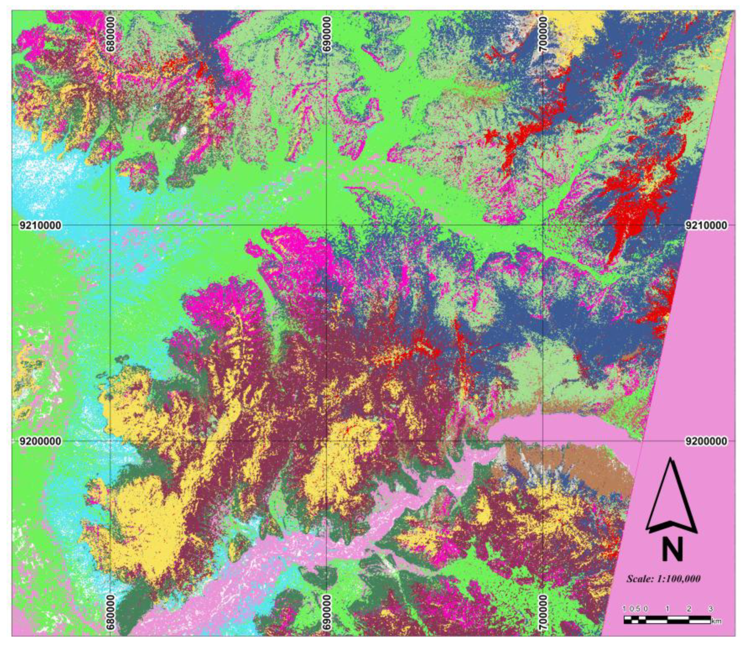
The classification maps obtained with Landsat 8, Sentinel-2, and ASTER show that all three sensors successfully identified the main lithological units of the study area. However, Landsat 8 showed the best classification performance, reflected in the highest overall accuracy, Kappa coefficient, and F1-score, making it the most suitable sensor for lithological mapping. Meanwhile, Sentinel-2 and ASTER provided complementary spectral information that contributed to the classification process and the geological interpretation of the identified units.
Figure 11.
Lithological classification using Landsat 8 image.

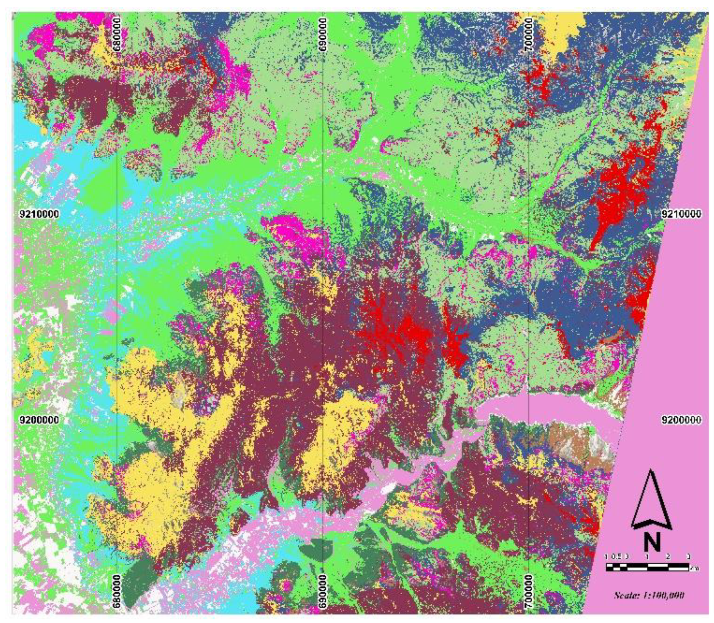
Figure 12.
Lithological classification using Sentinel-2 image.
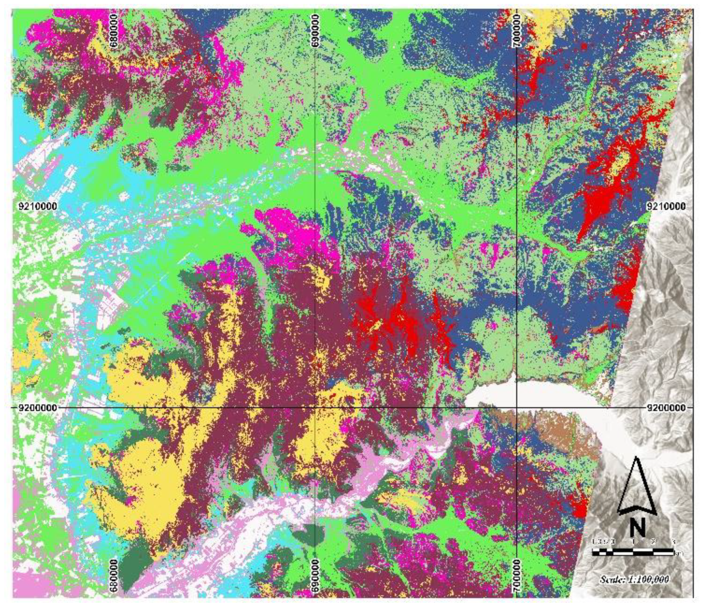
Figure 13.
Lithological classification using ASTER image.
4.4.2. Field-Observed Lithological Units
Table 3.
Field validation of lithological mapping.
| Point | Geological Mapping (INGEMMET) | Random Forest Classification | Field Lithology | Identified Geological Unit |
|---|---|---|---|---|
| 1 | Ki-i, chu | Ki-pa | Packstone Limestone | Ki-chu |
| 2 | Ki-i, chu | Ki-pa | Mudstone Limestone | Ki-pa |
| 3 | Ki-i, chu | Ki-pa | Limonite | Ki-i, chu |
| 4 | Ki-i, chu | Ki-pa | Packstone Limestone | Ki-Pa |
| 5 | Q-fl | Ki-g | Sandstone | Ki-G |
| 6 | Ki-g | Ki-g | Litharenite | Ki-G |
| 7 | Ki-g | Ki-pa | Shale | Ki-Pa |
| 8 | Ki-i, chu | Ki-pa | Quartzose Sandstone | Ki-i, chu |
| 9 | Ksp-gd | Granodiorite | Granodiorite | Granodiorite |
| 10 | Ksp-gd | Quartz Diorite | Quartz Diorite | Quartz Diorite |
| 11 | Ki-i, chu | Quartz Porphyry | Quartz Porphyry | Quartz Porphyry |
| 12 | Ksp-Gd | Diorite | Diorite | Diorite |
| 13 | P-ll | Llama | Andesitic Lava | Andesitic Lava |
| 14 | Ksp-gd | Granodiorite | Granodiorite | Granodiorite |
| 15 | Ksp-gd | Granodiorite | Granodiorite | Granodiorite |
| 16 | Ksp-gd | Granodiorite | Granodiorite | Granodiorite |
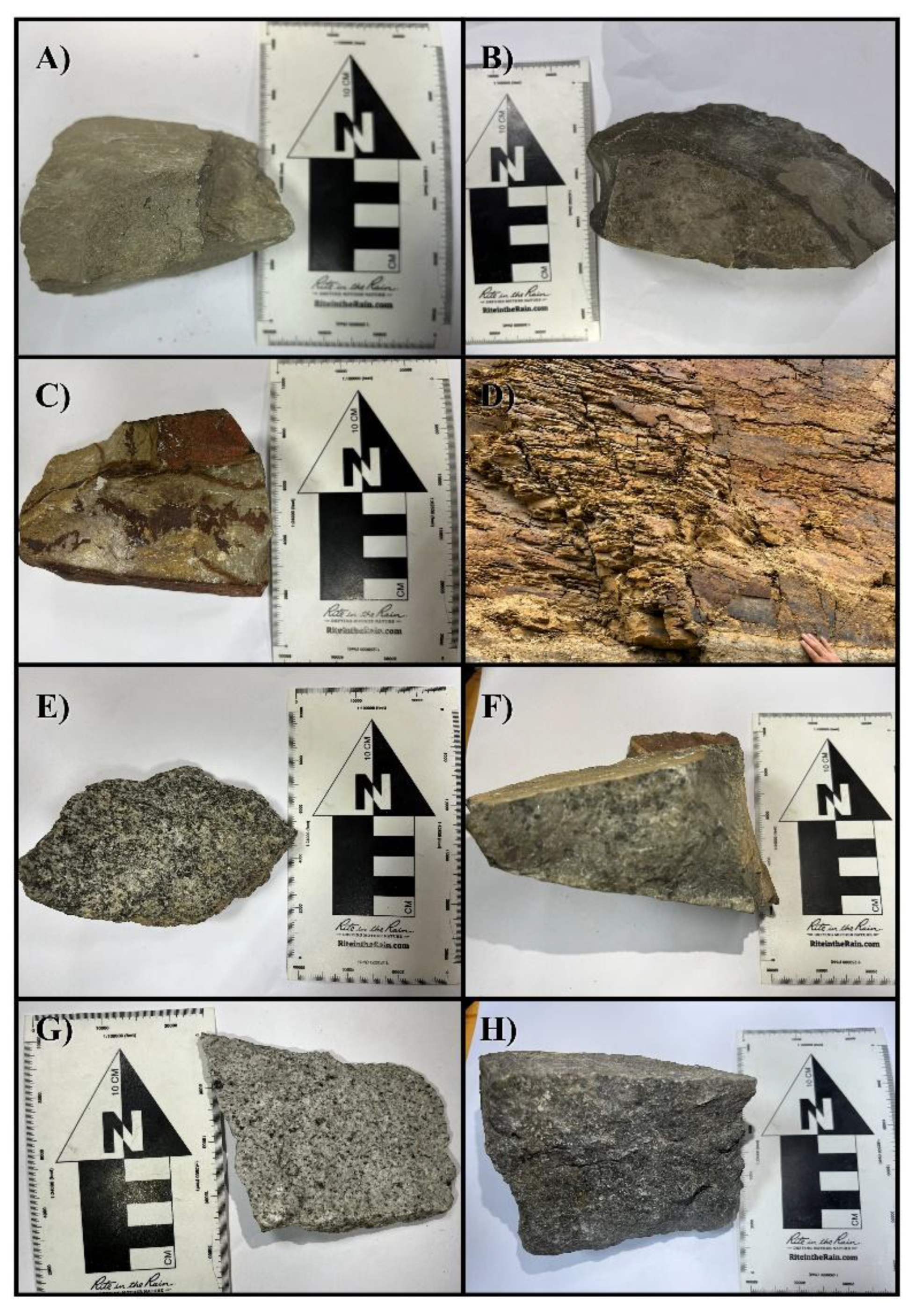
Table 2 compares the INGEMMET geological mapping, the classification obtained through Random Forest, the field observations, and the geological unit assigned based on sample analysis. In the sedimentary units (Points 1 to 8), the main differences appear between the Inca–Chúlec and Pariatambo Formations due to their lithological similarity. The limestones were classified as mudstone, wackestone, and packstone according to their fossil content and the proportion of carbonate matrix; mudstones present scarce fossils, whereas wackestones and, primarily, packstones show a higher fossiliferous content, facilitating their differentiation. Based on these characteristics, points 2, 4, and 7 were assigned to the Pariatambo Formation, points 1, 3, and 8 to the Inca–Chúlec Formation, and points 5 and 6 to the Goyllarisquizga Group due to the presence of sandstones and litharenites.
In the intrusive units (Points 9 to 16), the classification showed good correspondence with field observations. Granodiorites, quartz diorites, and diorites were identified; additionally, point 11 corresponds to a quartz-rich granitoid (quartz porphyry) and point 13 was identified as an andesitic lava. Finally, point 14 corresponds to a hornblende granitoid, characterized by its higher hornblende content. Overall, field verification supported and complemented the lithological mapping obtained through Random Forest.
Figure 14.
Field samples of the identified lithological units: A) Mudstone limestone (Chúlec Fm.), B) Bituminous limestone (Pariatambo Fm.), C) Litharenite (Goyllarisquizga Gr.), D) Shale (Pariatambo Fm.), E) Hornblende granodiorite, F) Quartz porphyry, G) Quartz diorite, H) Andesitic lava.
Figure 14.
Field samples of the identified lithological units: A) Mudstone limestone (Chúlec Fm.), B) Bituminous limestone (Pariatambo Fm.), C) Litharenite (Goyllarisquizga Gr.), D) Shale (Pariatambo Fm.), E) Hornblende granodiorite, F) Quartz porphyry, G) Quartz diorite, H) Andesitic lava.
4.4.3. Influence of Morphometric Variables on the Identification of Quaternary Deposits
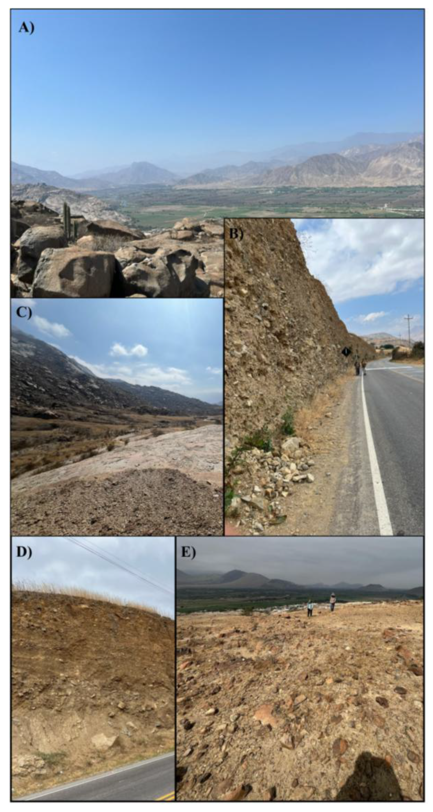
Elevation, derived from the Digital Elevation Model (DEM), was one of the most important variables in all three models, demonstrating that relief is a key factor for lithological discrimination in the study area. During field verification, it was observed that fluvial, alluvial, and eolian deposits exhibit a marked association with specific altitudinal ranges and geomorphological positions. Fluvial deposits are primarily distributed along river channels and recent terraces, alluvial deposits occupy piedmont zones and alluvial fans, whereas eolian deposits develop preferentially in relatively flat surfaces and sectors with lower slopes. This relationship between lithology and topography explains the high contribution of the elevation variable to the classification process.
The relevance of other morphometric variables, such as slope, the topographic wetness index (TWI), the topographic position index (TPI), and solar radiation (or surface index / insolation, SI), reinforces the influence of relief on the spatial distribution of geological units. Together, these variables accounted for between 44% and 48% of the total model importance, surpassing the individual contribution of several spectral attributes, which demonstrates that topographic information plays a fundamental role in the lithological mapping of the study area.
Figure 15.
Quaternary deposits observed during field verification: A) Fluvial deposit, B) Alluvial deposit, C) Alluvial deposit, D) Fluvial deposit, E) Eolian deposit.
Figure 15.
Quaternary deposits observed during field verification: A) Fluvial deposit, B) Alluvial deposit, C) Alluvial deposit, D) Fluvial deposit, E) Eolian deposit.
5. Discussion
The classification obtained through the Random Forest predictive model successfully discriminated the main lithological units of the study area. The greatest difficulties arose between the Inca–Chúlec and Pariatambo formations, due to the similarity of their lithological characteristics and, consequently, their spectral response. In contrast, sandstones, intrusive units such as granodiorites, quartz diorites, and quartz-rich granitoids (quartz porphyries), as well as Quaternary deposits, were consistently identified. In the latter, the incorporation of morphometric variables especially elevationimproved their discrimination by reflecting the close relationship between these units and relief characteristics.
Field verification supported these results by confirming that the differences between the Inca–Chúlec and Pariatambo formations are primarily due to the similarity of their lithologies. Likewise, it was observed that fluvial, alluvial, and eolian deposits occupy well-defined geomorphological positions, which explains the high contribution of morphometric variables to the model. Similarly, the continuity of sandstone outcrops and the distinctive lithological features of the intrusive units favored their proper classification. Together, these results demonstrate that the integration of spectral and morphometric variables using Random Forest, complemented by field verification, yields more reliable lithological mapping with stronger geological support.
6. Conclusions
The integration of Landsat 8, Sentinel-2, and ASTER images, DEM-derived morphometric variables, and the Random Forest algorithm allowed for reliable lithological mapping of the San Gregorio–Chepén sector. Among the evaluated sensors, Landsat 8 showed the best performance (OA = 76.1%, Kappa = 0.736, and F1-score = 76.8%), while Sentinel-2 and ASTER complemented the interpretation of the lithological units.
Morphometric variables played a fundamental role in the classification, contributing between 44% and 48% of the total model importance. Elevation was the most influential variable, demonstrating that relief is a determining factor for lithological discrimination, especially in the identification of Quaternary deposits.
Field verification confirmed the reliability of the generated mapping and allowed for the interpretation of the main discrepancies between the Inca–Chúlec and Pariatambo formations, which are associated with the similarity of their lithological characteristics. Overall, the results demonstrate that the integration of multispectral information, morphometric variables, and machine learning constitutes an effective methodology to support lithological mapping and complement conventional geological mapping.
References
- Ccallo, W.; Weimin, G.; Mamani, M.; Jaimes, F. Geocronología U-Pb y litogeoquímica de los principales segmentos del Batolito de la Costa. In Proceedings of the XIX Peruvian Geological Congress, Lima, Peru, 2018; pp. 101–105. [Google Scholar]
- Wilson, J. Geología de los Cuadrángulos de Jayanca, Incahuasi, Cutervo, Chiclayo, Chongoyape, Chota, Celendín, Pacasmayo y Chepén; Boletín A-38; INGEMMET: Lima, Peru, 1985; pp. 42–43.
- Rivera, M.; Monge, R.; Navarro, P. Nuevos datos sobre el volcanismo Cenozoico (Grupo Calipuy) en el norte del Perú: departamentos de La Libertad y Áncash. Bol. Soc. Geol. Perú 2005, 99, 7–21. [Google Scholar]
- Roy, D.; Wulder, M.; Loveland, T.; Woodcock, C.; Allen, R.; Anderson, M.; Helder, D.; Irons, J.; Johnson, D.; Kennedy, R.; Scambos, T.; Schaaf, C.; Schott, J.; Sheng, Y.; Vermote, E.; Belward, A.; Bindschadler, R.; Cohen, W.; Gao, F.; Hipple, J.; Hostert, P.; Huntington, J.; Justice, C.; Kilic, A.; Kovalskyy, V.; Lee, Z.; Lymburner, L.; Masek, J.; McCorkel, J.; Shuai, Y.; Trezza, R.; Vogelmann, J.; Wynne, R.; Zhu, Z. Landsat-8: Science and product vision for terrestrial global change research. Remote Sens. Environ. 2014, 145, 154–172. [Google Scholar] [CrossRef]
- García, E.; Báscones, A.; Ferrer, M.; Suárez, M.; Colmenero, E.; Cruz, J.; Pereira, I. Cocientes de bandas espectrales ASTER para la diferenciación litológica en formas del relieve de baja pendiente (NW de la Cuenca del Duero, León, España). Geogaceta 2023, 73, 79–82. [Google Scholar] [CrossRef]
- Gobierno de España. El programa Copernicus Aplicado a la Producción y Gestión de Información Geográfica; Instituto Geográfico Nacional de España: Madrid, Spain, 2018. [Google Scholar]
- Serra, M.; Solorza, R.; Aumassanne, C.; Salcedo, A. Geomática Aplicada al Análisis Morfométrico y Geomorfológico en Cuencas; INTA: Argentina, 2025. [Google Scholar]
- Rosales, J.; Apaza, H. Análisis de imágenes satelitales Landsat 8 por componentes principales y MNF para la detección de zonas del derrame de petróleo Repsol en la Costa Peruana. Tecnohumanismo 2022, 2, 172–189. [Google Scholar] [CrossRef]
- Yirenkyi, S.; Boateng, C.; Ahene, E.; Danuor, S. Identificación automática de litología en cráteres de impacto de meteoritos mediante algoritmos de aprendizaje automático. Sci. Rep. 2024, 14, 14360. [Google Scholar] [PubMed]
- Aoki, Y.; Furuya, M.; De Zan, F.; Doin, M.P.; Eineder, M.; Ohki, M.; Wright, T.J. L-band Synthetic Aperture Radar: Current and future applications to Earth sciences. Earth Planets Space 2021, 73, 56. [Google Scholar] [CrossRef]
Disclaimer/Publisher’s Note: The statements, opinions and data contained in all publications are solely those of the individual author(s) and contributor(s) and not of MDPI and/or the editor(s). MDPI and/or the editor(s) disclaim responsibility for any injury to people or property resulting from any ideas, methods, instructions or products referred to in the content. |
© 2026 by the authors. Licensee MDPI, Basel, Switzerland. This article is an open access article distributed under the terms and conditions of the Creative Commons Attribution (CC BY) license (http://creativecommons.org/licenses/by/4.0/).
Copyright: This open access article is published under a Creative Commons CC BY 4.0 license, which permit the free download, distribution, and reuse, provided that the author and preprint are cited in any reuse.