

Submitted:
07 November 2026
Posted:
09 November 2026
You are already at the latest version
Abstract
Quantum interpretations differ in their accounts of reality while often predicting identical observations. We examine their relative plausibility under eight alternative judgments emphasizing economy of universal dynamics, definite physical configurations, physical selection of outcomes, states and events relative to interacting systems, quantum states as expectations, time symmetry and dependence on future boundary conditions, correlations between measurement settings and underlying variables, or a balance of these considerations. For each judgment, we retrospectively assign illustrative prior probabilities across ten accounts according to their perceived explanatory merits. Bayesian updating multiplies these weights by experimental evidence factors and rescales each distribution to total 100%.Discrimination requires different probabilities for common observable records, with noise and calibration uncertainties sufficiently constrained. The calculations show that different Bohmian entry times can yield identical detector probabilities, identify conditions for distinguishing collapse from environmental dephasing, and derive a spatial test separating two specified collapse laws. A likelihood reconstructed from published radiation summaries of the XENONnT experiment gives an approximate evidence factor of 0.3245, relative to ordinary quantum predictions, for an equal mixture of specified white-noise continuous spontaneous localization and regularized Diósi–Penrose models. Under the stated parameter priors, a starting collapse benchmark weight of 45% falls to 20.98%, while Bohm's rises from 20% to 28.73%. Accounts with matched observable predictions and parameter assumptions retain their relative odds. Three entries without calculated likelihoods receive assumed neutral evidence factors. The estimates depend on the initial judgments, model coverage, parameter priors, and likelihood reconstruction.
Keywords:
quantum interpretations
; quantum ontology
; empirical equivalence
; Bayesian model comparison
; objective collapse
; matter-wave interferometry
1. Introduction
Quantum theory predicts experimental observations with extraordinary success, yet its interpretations give different accounts of what happens in the physical world. In Everett’s account, the alternatives persist in branches of a universal quantum state. Bohmian mechanics adds actual particle configurations and their trajectories. Physical collapse theories change the dynamics so that one alternative survives. Relational and QBist approaches reconsider the meaning of states and outcomes. We would like to know how much confidence each account deserves and what observations could change that confidence.
The familiar textbook treatment provides a useful point of comparison. An apparatus produces a definite reading with a probability given by the Born rule; subsequent predictions use a state conditioned on that reading. This treatment is often associated with Bohr and the Copenhagen tradition. Bohr emphasized the experimental arrangement and the classical terms in which results are communicated [1,2]. We use those concerns to frame the comparison, while defining the textbook measurement rule explicitly below. A stochastic mechanism that changes the motion of matter between measurements is a further physical proposal, with additional predictions that can be tested.
The distinction matters for the numerical assessment. Several interpretations reproduce the textbook probabilities, so the observations used here leave their relative odds unchanged. The specified spontaneous-collapse models predict additional radiation. The same observations can therefore change their odds relative to the textbook reference. A preference for Everett or Bohm over that reference must have other grounds wherever their predicted observations agree.
We represent such grounds through eight alternative sets of starting probabilities. Each gives greater weight to a stated explanatory consideration, such as economy of the dynamical law or definite physical configurations. The percentages express illustrative judgments made for this analysis. Applying the same experimental evidence to each set shows which preferences the evidence changes and which it leaves intact. The eight sets are separate assessments; combining them would require an additional judgment about their relative weights.
Work on interpretation, theory rivalry, and empirical underdetermination provides the background for this comparison [3,4,5]. Pessoa describes eight relations between interpretations and experiments [6]. Those eight relations are distinct from the eight starting judgments used for our probability calculation. Fraser and Vickers identify claims about reality shared by Everettian, Bohmian, and Ghirardi–Rimini–Weber (GRW) theories [7]; related work examines quantum ontology, including the material entities that constitute an apparatus and its records [8,9]. Here we follow a physical claim through a specified apparatus to the probabilities of its recorded outcomes.
The claims under comparison concern different aspects of a theory. A claim that particles follow definite paths concerns what exists and how it moves. A claim that physical collapse occurs concerns the evolution of the quantum state. Within a collapse theory, matter might be represented by particles, a continuous density, or discrete events. Even after those choices have been made, the rate and length scale of collapse remain to be specified. GRW, continuous spontaneous localization (CSL), and regularized Diósi–Penrose (DP) theories prescribe particular dynamical laws. GRW matter density and GRW flashes illustrate a different choice: they associate different material contents with the same stochastic wave-function evolution [9].
An experiment may answer one of these questions while leaving the others open. Surviving interference demonstrates accessible coherence under the conditions tested. Everettian and equilibrium Bohmian calculations can both predict it. Likewise, a measured collapse rate might favor a particular dynamical law while leaving several accounts of matter compatible with the observations. The probability calculation must specify the level at which its alternatives differ.
Bell experiments constrain the conjunction of local causality and statistical independence between measurement settings and underlying physical variables. The observed violations exclude models satisfying both assumptions [10]. Any account reproducing the correlations must relinquish at least one. The Pusey–Barrett–Rudolph theorem restricts overlapping distributions over underlying states under preparation independence [11], and the Kochen–Specker theorem excludes the relevant noncontextual assignments of definite values [12]. These results narrow the admissible descriptions of reality. Numerical odds among the surviving accounts require additional assumptions about their probabilities for the observations.
The theoretical survey and the probability calculation serve different purposes. Supplement S1 registers eleven formulations or reference models, which yield 55 pairs and 165 triples for possible comparison. It also groups the wider literature into twelve overlapping interpretive families. The statistical calculation uses ten mutually exclusive entries, defined in Supplement S2, so that their probabilities can sum to one. Neither the number of families nor the number of registered comparisons determines a candidate’s starting weight.
Three worked comparisons establish how these distinctions affect an experiment. The arrival calculation asks whether different particle trajectories lead to different detector records [13,14,15]. The memory calculation asks whether a loss of interference can be attributed to physical collapse when environmental noise can produce the same effect [16]. The spatial calculation asks whether measurements at several separations can distinguish two collapse laws after their parameters have been fitted. Each comparison includes the preparation, recorded outcome, relevant uncertainty, and experimental effort needed to resolve a difference.
The numerical assessment then uses published radiation information and examines released interference records for possible inclusion. The radiation summaries permit an approximate reconstruction of the likelihood, meaning the probability of the observed data as a function of the model and its parameters. The interference reconstruction fits inadequately without a fuller account of ordinary contrast loss, so it is excluded from the probability update. We report how the radiation result depends on the starting judgments, parameter priors, reconstruction choices, and range of collapse laws included.
2. Methods
2.1. The Textbook Measurement Reference
For the reference calculation, the system evolves according to ordinary quantum dynamics between specified measurement operations. Each operation assigns Born-rule probabilities to possible apparatus records and a conditional state for subsequent predictions. Quantum instrument theory gives this prescription for general measurements [17]. For an ideal projective measurement, conditioning reduces the state to the subspace associated with the recorded result. This is the sense of measurement collapse used for the reference.
The reference does not introduce a universal collapse rate or localization length. Those parameters belong to dynamical proposals such as CSL and DP. It also permits a detector or memory to be included in the quantum system when its interaction can be controlled coherently. Merely correlating a system with a reversible memory therefore supplies no additional rule that destroys their joint coherence.
Bohr’s account motivates the attention to the experimental arrangement [1,2]. The reference defined here is a precise prescription for probabilities, without claiming to exhaust Bohr’s historical position or every Copenhagen interpretation. In the statistical catalogue, the Operational entry adds the judgment that this operational description is explanatorily complete. Its prior weight belongs to that judgment. We do not add a separate Bohr entry with another share of the same starting probability.
2.2. Formulations and Observable Records
A formulation must specify what its physical entities are, how they evolve, and how their state produces the records of an apparatus. An interpretation’s name alone leaves some of these choices open. Let M denote a specified formulation and let C describe the experimental procedure: preparation, controls, detector operation, observation time, and the rule for retaining trials. Its prediction is a probability distribution over the possible records,
The set includes failures to detect. A rule that discards trials must be included in both the prediction and the analysis. If the candidates predict different detection efficiencies, the number of failures is evidence alongside the times of successful detections.
Two formulations are empirically equivalent on a stated collection of experiments when they assign the same distribution to the records of every experiment in that collection. The allowed interventions matter. Two models can predict equal decay during uninterrupted storage and different responses to an echo pulse. Equivalence established for passive observation does not automatically extend to controlled experiments.
When evidence from several experiments is combined, each model must use consistent values of its universal physical parameters. A localization length, for example, has one value across materials and apparatuses. Detector efficiencies and ordinary backgrounds may vary, with their uncertainty constrained by calibration. A joint likelihood must preserve any correlations and count shared calibration information once. Supplement S1 shows how fitting experiments separately can conceal incompatible values of a common parameter.
2.3. Distinguishability and Experimental Uncertainty
For fixed parameters, the difference between the predicted records can be measured by total variation:
The supremum is over measurable events. Identical predictions give zero distance; mutually singular distributions give distance one, allowing perfect discrimination of the known alternatives from one record. With equal prior probabilities, the smallest average probability of choosing incorrectly from that record is [18]. The optimization is over decisions made from the record of the fixed apparatus.
Uncertain parameters give each candidate a range of possible predictions. If the ranges overlap, some allowed choices predict exactly the same observations. Even ranges that do not intersect may approach each other so closely that a fixed number of measurements cannot reliably distinguish every allowed pair. The memory and spatial calculations identify calibration conditions that leave a positive gap between the predictions and derive sufficient numbers of repetitions. Their error bounds describe the frequency of wrong decisions over repeated experiments.
A physical quantity shared by several ontologies can be partially identified. Suppose the total coherence-loss rate is and independent calibration restricts the environmental part to –. If environmental dephasing and collapse are the only additive contributions, the collapse rate lies between and . The interval constrains collapse under the additive assumption, while several accounts of that collapse may remain [19]. Supplement S1 gives the general construction and its coverage conditions.
2.4. From Evidence to Relative Probabilities
The probability update combines two different assessments. A prior gives the relative plausibility assigned to an account before the selected data are used. A likelihood states how probable those data would be if that account and its physical assumptions were correct. Bayes’ rule changes the prior odds by the ratio of the likelihoods.
Let D be the data and B the background information already used to define the candidates and their priors. For two formulations with nonzero prior probabilities, Bayes’ rule gives
The ratio of the models’ marginal likelihoods is the Bayes factor [20]. A value of one leaves their relative odds unchanged. It does not make their probabilities equal. For example, starting weights of 45% for Everett and 15% for Bohm retain a three-to-one ratio when their likelihoods agree. Both percentages can rise if the observations reduce support for a third candidate.
Physical parameters, such as a collapse rate, and apparatus parameters, such as detector efficiency, may be uncertain. The latter are called nuisance parameters because their values affect the comparison without being its principal subject. A model’s marginal likelihood averages its data probabilities over the stated prior distribution for all these parameters, denoted collectively by :
Two models can permit the same range of observations and nevertheless receive different marginal likelihoods if their parameter priors give different weights to those predictions. Equal marginal likelihoods require matched probability assignments over the observable distributions, including nuisance effects.
Within each starting assessment, we multiply every prior weight by its model likelihood and divide by the sum of all the resulting weights. This normalization makes the updated probabilities sum to one. For account i in judgment scenario s, with prior weight ,
The catalogue must contain mutually exclusive entries for this interpretation to hold. Dividing an entry into empirically identical variants should preserve its total prior weight. A broad collapse family also requires an allocation among its component laws; the evidence for those laws is averaged according to that allocation.
A probability ranking is useful only if the candidate models adequately describe the observations. The best fit among several poor models can still be poor. In an interference experiment, an added collapse term may improve the fit by absorbing ordinary contrast loss omitted from the apparatus model. We check this possibility before deciding whether the released interference records can enter the update.
2.5. The Eight Judgments and the Numerical Catalogue
Table 1 identifies eight explanatory judgments and the account most favored by each. Each judgment determines a complete allocation across the ten accounts, supplied in Supplement S2. For example, giving priority to a universal dynamical law motivates the 45% Everett weight in A; giving priority to definite configurations motivates the 45% Bohm weight in B. The remaining probability is distributed among the other accounts according to their perceived explanatory merits.
The numerical choices are ours. The cited literature explains the positions, but supplies no rule that uniquely converts those commitments into percentages. We constructed the profiles retrospectively to examine sensitivity to philosophical and theoretical preferences, without a survey, independent elicitation, or validated scoring rule. For the calculation, each profile is treated as a hypothetical assessment made before incorporating the selected radiation data. Any data already used in assigning a prior would otherwise be counted twice. Varying the profiles is a form of prior sensitivity analysis [21].

Table 1.
The eight starting judgments. The favored entry and its weight identify each profile; the remaining weights are specified in Supplement S2.
Table 1.
The eight starting judgments. The favored entry and its weight identify each profile; the remaining weights are specified in Supplement S2.
| Scenario | Judgment given greatest weight | Favored starting entry |
| A | Economy of a universal dynamical law [22,23] | Everett, 45% |
| B | A definite, objective world of individual outcomes [24,25] | Bohm, 45% |
| C | Physical selection of one outcome [26,27] | CSL/DP benchmark, 45% |
| D | States and events relative to interacting systems [28,29] | Relational, 45% |
| E | Limits on what a quantum state describes [2,30] | QBism, 35% |
| F | Time symmetry and future boundary conditions [31] | Retrocausal, 40% |
| G | Dependence between settings and underlying variables [32] | Superdeterminism, 35% |
| H | An illustrative balance of the competing considerations | Everett and Bohm, 25% each |
Six catalogue entries reproduce the textbook reference probabilities for the radiation observations: Everett with Born weights, equilibrium Bohm, the specified relational and QBist assignments, consistent histories for these records, and the operational account. With matched physical and nuisance assumptions, all six have evidence factor one relative to that reference. Consistent histories assigns probabilities within compatible frameworks [33]. Its catalogue entry, like the operational entry, represents a particular explanatory position. The equal likelihoods apply to the specified implementations and observations; other versions need their own probability calculations.
The collapse benchmark is an equal mixture of mass-proportional white-noise CSL at nm and regularized white-noise DP in the Diósi convention. We use priors uniform in on and in on . These ranges are chosen for the sensitivity analysis. They include effects so weak that they may be inadequate to explain definite macroscopic outcomes; we impose no additional adequacy criterion. The calculated support therefore applies to the specified dynamical benchmarks.
Retrocausal, Superdeterminism, and Other have no calculated likelihood for the selected experiment. We therefore report two calculations. The seven-entry calculation asks for probabilities conditional on the modeled alternatives alone. The ten-entry calculation retains all the original prior weights and assigns a neutral evidence factor of one to each unmodeled entry. This convention makes a complete table possible but provides no experimental assessment of those three accounts. It is particularly consequential when one of them has a large prior weight.
Some physical proposals also combine commitments that appear in several named interpretations. A trajectory theory might use future boundary conditions, for example. Supplement S2 assigns such hybrids once, under Other, unless an explicitly redefined catalogue replaces an existing entry. This prevents the same proposal from receiving probability under several labels.
2.6. Evidence Included and Likelihood Reconstruction
The arrival, memory, and spatial calculations describe prospective tests. Their simulated records verify theoretical predictions and supply no observed counts for the probability update. Existing Bell and local-friendliness experiments constrain combinations of premises; the Pusey–Barrett–Rudolph and Kochen–Specker theorems constrain possible model constructions. These restrictions matter when defining admissible candidates. Numerical odds among surviving implementations require their different probabilities for the observations.
Every candidate in the central update is assessed against the same published XENONnT radiation summaries [34]. The germanium counts reported by Donadi and colleagues [35] enter a separate comparison of DP with ordinary predictions. Adding them to the full catalogue would also require the corresponding germanium signal under CSL, which has not been calculated here.
The full XENONnT likelihood, including uncertainty in the detector and backgrounds, was unavailable to this analysis. We approximate it from the reported limits and significances, interpolate between those constraints [36], and specify how it decays beyond them. This reconstruction requires assumptions about how the reported statistical quantities relate to likelihood ratios [37]. Averaging over nuisance parameters requires further information [20,38]. Supplement S2 states the approximations and examines how changing them affects the result.
The germanium study reports 576 observed counts, a simulated ordinary background of 506, and signal coefficient in the authors’ Penrose convention. Its rate is times the Diósi convention adopted here. We accordingly use the Poisson mean , holding the simulated background fixed as an approximation. The published bound uses an effective offset of 508 after one-count inferential adjustments to background and signal. Supplement S2 reproduces that construction separately and examines both the offset and assumed background uncertainty.
If and are the resulting approximate evidence factors, the benchmark factor is
The two terms use the same radiation data and the same reference likelihood. Their average represents equal prior weight for the two alternative collapse laws. In the separate DP diagnostic, xenon and germanium observations are independent and are combined at a common DP parameter before that parameter is integrated out. The older public XENONnT electronic-recoil sample overlaps the revised analysis and therefore supplies no independent additional observations [39]. We also evaluate the sodium interference records with the released apparatus calculation [40,41] to determine whether their fit is adequate for inclusion.
2.7. Computational and Editorial Assistance
OpenAI ChatGPT was used for literature discovery and organization, development and checking of mathematical arguments, generation of computational code, numerical verification, analysis of public data and published statistical information, and assistance in drafting and editing the manuscript. The author retains responsibility for evaluating AI-assisted material and for the accuracy, interpretation, and final submission of the work, including the entire text in its final form.
3. Arrival and Detection Times
Bohmian mechanics assigns trajectories to particles even when no detector is present. Two spin mixtures can share the same density operator yet have different distributions of the times at which those trajectories enter a region. The experimental question is whether one detector, operated identically on both mixtures, records those undisturbed entry times. If it did, the observed distributions would differ. We calculate both the undisturbed motion and the detector’s response.
3.1. Spin Preparations and Record Probabilities
Prepare a particle in a fixed spatial state . In ensemble Z, choose spin or with equal probability; in ensemble X, choose or with equal probability. Their average density operators coincide:
Neither the detector nor its initial environment receives the preparation label. For the common positive-operator-valued measure (POVM) , which specifies the probabilities of recorded outcomes [17],
The equality includes spin-sensitive detectors and sequences of measurements with feedback [42]. Its application to Bohmian mechanics additionally assumes quantum equilibrium, a common independent apparatus configuration, linear composite evolution, and a fixed pointer-reading rule [24,25,43]. An Everettian formulation using Born weights gives the same probabilities; the justification of those weights is a separate question [44].
Consider the ground state of an isotropic harmonic trap, with oscillator length . The Pauli guidance current including its magnetization contribution gives velocity for spin direction [45]. For , trajectories rotate in the plane; for , x remains constant. With no detector present, ask when a trajectory first enters during one period . Initial positions have density . Writing , the entry probabilities are
Supplement S1 derives the full time distributions, including entry at zero and failure to enter. Their total variation distance is
At , , , and . Their probabilities at time zero coincide, while later arrivals and failures differ. This effective Pauli model assumes and does not describe its remote Gaussian tails relativistically. With the magnetization current omitted, the trajectory discrepancy disappears. The common-measurement equality (8) holds in either case.
Let be the undisturbed arrival distribution and the record distribution of one common measurement for each pure spin preparation. Averaging each pair in (8), then applying convexity and the triangle inequality, gives
The midpoint record generator attains the bound in the unrestricted POVM class. It attains the distributional bound by generating state-independent random records. Such a construction provides no measurement of an individual arrival. The bound gives an exact instance of the established approximation obstruction [14,15]. At , every common measurement misses at least one target distribution by at least 0.144615.
3.2. Absorbing Detector and Count Test
The detector occupies , is switched on at zero, and absorbs at a finite rate . The trap remains in place. Absorbing potentials are established detector models [46,47,48]. With the trap Hamiltonian, define
The first-click operator is , and the no-click operator is . The time integral of the first-click operator plus the no-click operator is the identity. The probability of a click by t is
It is the same for both ensembles and for all four spin orientations. The Hamiltonian and rate operator do not commute, so their sum must be retained in the exponential. Supplement S1 gives the normalized instrument and oscillator-basis calculation.
At and , the calculated click probability is 0.370007 for both ensembles. It is close to the Z entry probability, 0.367879, but far above the X entry probability, 0.078650. Comparison with Z alone would therefore give a misleading impression of what the detector measures. Increasing from 4 to 16 reduces the click probability from 0.632364 to 0.568032, further illustrating the effect of the detector on the dynamics. Supplement S1 reports basis sensitivity for these theoretical calculations.
A count test can evaluate the proposed identification of clicks with undisturbed arrivals. Allowing an error of 0.02 in the difference between ensemble click probabilities, the illustrated design requires 152 trials per ensemble for false-positive probability at most 0.04 and power at least 0.80, conditional on calibration. Calibration trials are additional. Equilibrium Bohmian mechanics and the ordinary measurement formalism both predict the null difference; the alternative tested is the proposed arrival-to-detection identification.
A related issue arises when waveguide populations are converted into inferred tunneling speeds. The recent dispute concerns the validity of that conversion [49,50]. Applying a common conversion to identical record distributions preserves their statistical equality. Supplement S1 discusses the apparatus objections and associated preprints in more detail.
4. Distinguishing Collapse from Environmental Noise
4.1. A Reversible Record and an Interference Measurement
A memory can become correlated with a quantum system while the combined state remains coherent. If that interaction can be reversed, interference tests whether coherence survived storage. Prepare a superposition, correlate its alternatives with two memory states, wait, and coherently undo the recording interaction. An interference measurement then compares the returned state with the original superposition. Simply reading the two memory labels gives the same frequencies for an intact superposition and a collapsed mixture.
In the textbook reference of Section 2.1, this reversible correlation belongs to the controlled quantum evolution. Assigning irreversible physical collapse to it adds a hypothesis about when coherence is destroyed. The calculation below tests that hypothesis against ordinary dynamics with environmental noise. Its result cannot be attributed to Bohr merely by calling the intermediate correlation a measurement.
Let and denote the two correlated system–memory states. Each pair is treated as one logical state, indicated by the subscript L. An uncontrolled environment may also become correlated with them, acquiring states and . Their overlap, , determines how much coherence remains accessible to measurements on the system and memory. If physical collapse additionally reduces that coherence by a factor , the two reduced states are
Their diagonal elements give equal probabilities for the two memory labels. Their off-diagonal elements determine the interference. The trace distance, , quantifies the largest difference in outcome probability available to a suitable measurement. When the environment perfectly distinguishes the alternatives, and measurements on the system and memory cannot distinguish these reduced states. The connection between retained path information and interference is established [51,52]. Equilibrium Bohmian mechanics gives the same interference probabilities as ordinary unitary evolution for the complete apparatus.
4.2. Echo Response and Dephasing
A spin echo reverses phase accumulation from a constant frequency offset [53]. Here the pulse exchanges the complete system–memory states halfway through storage, with a final exchange restoring their labels. Let distinguish the branches and suppose their reduced state obeys
The frequency offset is constant during a trial; is ordinary Markov dephasing, and is an additional effective collapse rate for the chosen geometry. A Markov description treats the environment as memoryless over the times considered. The effective depends on the physical mass distribution. Its relation to an elementary CSL rate must be derived for that geometry.
The echo cancels the phase from , but the surviving coherence is . Only the sum of the environmental and collapse rates appears. Dephasing at consequently gives the same records as dephasing at combined with collapse at . In the adopted model these choices have the same generator, so further logical pulses or adaptive measurements cannot distinguish them. More repetitions would estimate the total rate more precisely while leaving its division between the two causes unresolved.
The conclusion depends on the environmental model. A microscopic environment can respond to control in a way that an intrinsic collapse process does not, even when both give exponential decay during uninterrupted storage [16]. For example, a static Cauchy distribution of frequency offsets and Markov dephasing give the same free decay; an ideal echo reverses the former. Supplement S1 derives this example. A reduced generator must therefore describe the environment’s response to the permitted controls as well as its free evolution.
4.3. Calibration Bounds and Trial Counts
Independent calibration can restrict the ordinary noise enough to make the two explanations distinguishable. Repeat the storage-and-echo sequence and measure interference between the logical states. Assign score 1 to the positive outcome, 0 to the negative outcome, and to a flagged readout failure, so every launched trial contributes. If efficiency is independent of the outcome, let , with , combine efficiency and contrast. A possible imbalance or remaining bounded error contributes , with . The predicted mean score is
Losses that depend on the branch require a separate model or a justified allowance within b. Independent calibration restricts the ordinary rate to . To guarantee discrimination throughout that interval, compare the smallest mean allowed by ordinary unitary evolution with the largest mean allowed by collapse at rate . Their difference is
A positive g separates the means for every allowed choice. If and the calibration bounds are time independent, its maximum occurs at
Hoeffding’s inequality [54] gives a test with false-positive probability at most and power at least when
This includes failures through the bounded score. Supplement S1 supplies the threshold, boundary cases, and the separate calibration-error allowance.
For the illustrative bounds , , , and , the best time under equal trial cost is and the gap is 0.155634. Taking and requires 194 test trials. Calibration failure probability at most 0.01 raises the overall false-positive bound to 0.05 and gives unconditional power at least 0.79 when the calibration guarantee covers both hypotheses. These figures specify a prospective apparatus. The echo estimates ; interpreting an excess as collapse requires the separate calibration of .
5. Comparing Ordinary Dynamics, CSL, and DP at Five Separations
Suppose coherence decays faster than independently characterized ordinary processes can explain. The dependence of that excess on the separation of the branches provides another test. CSL and regularized DP both predict greater loss at larger separations, so observing that trend alone would leave both available. A discriminating measurement must resolve a shape that one law cannot reproduce with any consistent choice of its parameters and the allowed ordinary background.
The experiment prepares two narrow center-of-mass wave packets, holds them at a fixed separation, recombines them, and records a binary interference outcome. Five separations are used with the same object and readout procedure. A Gaussian intrinsic mass density with total mass m and width a makes the comparison analytically tractable. The width a describes the mass distribution within the rigid object; the center-of-mass packets are separately assumed narrow. For and , the established generators [55,56] give
Both vanish at by continuity. The CSL reference mass is . The DP normalization is times the Newtonian double integral of the difference between the smeared branch densities. This convention is matched to the radiation analysis. Supplement S1 derives the kernels and specifies their domain.
Let the ordinary rate be , with unknown coefficients fixed across separations within each candidate. The total ideal rate is , with . The ideal positive interference probability is . A rate residual bounded by covers departures from the ideal mass geometry and ordinary background; a probability allowance covers preparation and readout. Both allowances require independent physical characterization.
5.1. Five-Separation Identity
Choose , for . The actual separations are . At zero separation, distinct internal memory states have the same mass distribution. Define
Each cancels the constant and quadratic background. Ordinary dynamics alone gives . For CSL, with ,
The identity holds for every allowed CSL strength and localization length, including values obtained by fitting.
For DP, set and . Then . Normalizing the weight by gives a probability measure w, for which
The variance is positive because q varies over a set of positive weight. The single-exponential and mixture distinction [57] therefore separates these collapse laws: all five ideal DP rates cannot be reproduced by a CSL fit with a constant and quadratic background.
Let for a specified DP curve. Perturbing every rate by at most changes W by at most . Every curve with must therefore differ at one or more settings by at least
This lower bound on the maximum rate error need not be attained by the best fit. With statistical rate error and residual allowance , the condition suffices to separate the candidate ranges on the simultaneous confidence event. Supplement S1 derives that event, the trial counts, and the small-separation behavior. The rate distinction becomes eighth order in the separation scale when all separations are small.
5.2. Precision and Experimental Resources
For the illustrative Gaussian object with , nm, and nm, choose separations approximately 0, 894, 1265, 1549, and 1789 nm. With the stated background, the calculation gives and . A numerical CSL fit achieves maximum error , close to the certified bound. Its fitted localization length is 281.14 nm and its elementary rate is . Global optimality of this numerical fit has not been established.
With the error allowances stated in Supplement S1, the sufficient bound is 737,559,121 trials per setting at a storage time of 16.663 s: about trials in all, or 1,947 years of serial storage alone. A separate relative-entropy bound shows that even ideal calibration requires at least about trials per setting for both decision errors to be at most 0.05 at these settings and time. That is about 7.2 years of serial storage. The sufficient bound is conservative. The necessary bound applies to this design with equal trial allocation; different apparatuses or optimized protocols require separate resource estimates.
Figure 1.
Five-separation comparison for the Gaussian-body benchmark. The DP rates and a fitted CSL curve are nearly coincident; the inset shows the residual. The right panel gives the certified rate distinction as the spacing changes. Both fits include constant and quadratic ordinary backgrounds. The figure shows theoretical rates and design bounds.
Figure 1.
Five-separation comparison for the Gaussian-body benchmark. The DP rates and a fitted CSL curve are nearly coincident; the inset shows the residual. The right panel gives the certified rate distinction as the spacing changes. Both fits include constant and quadratic ordinary backgrounds. The figure shows theoretical rates and design bounds.
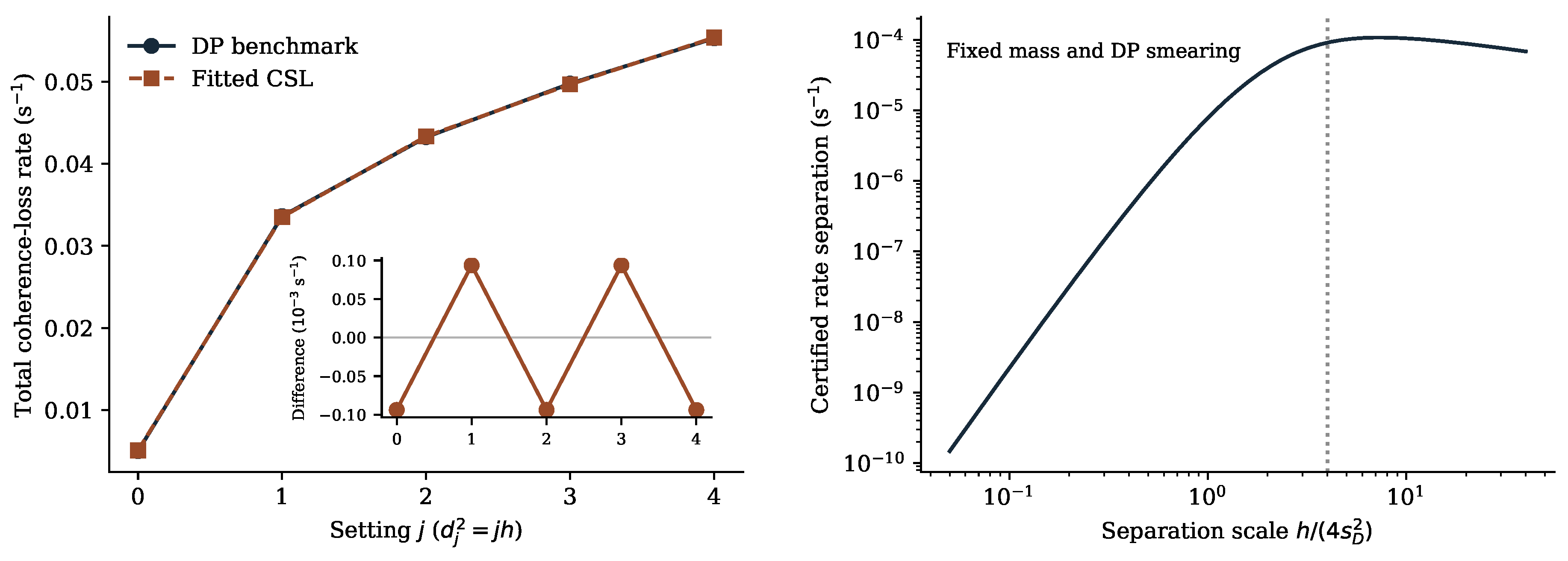
For the specified Gaussian geometry, a positive W that exceeds the error allowances would exclude both the fitted constant-plus-quadratic background alone and the single-scale CSL alternative. Further physical causes would remain possible. The DP kernel can be expressed as a mixture of Gaussian localization kernels, each realizable through ordinary random momentum kicks. An unobserved noise process can therefore produce the same loss of coherence. Supplement S1 constructs such a process; related work examines different physical processes giving the same collapse kernel and the dependence on geometry [58]. Measurements at different masses and environmental conditions, together with radiation or heating observations, could restrict those explanations. Changing the intrinsic mass profile also requires a new calculation, since the identity is exact for the Gaussian profile used here.
7. Experimental Evidence and Present Estimates
7.1. Interference and Radiation Observations
Pedalino and colleagues observed interference of sodium nanoparticles containing more than 7,000 atoms, with masses above 170,000 Da [40]. A collapse law predicts the interference remaining at the experimental mass, separation, and flight time. Under a specified apparatus model, parameters predicting too little contrast can be excluded. The observed survival of coherence is compatible with several ontologies.
Using the released data and code [41], we evaluated 95 scans comprising 3,895 positions and 10,772,714 detected counts. At the released phase and apparatus settings, the authors’ mass- and velocity-averaged Talbot–Lau calculation gives Pearson discrepancy about 44,892 and an apparent likelihood maximum near at nm. The large discrepancy shows that our fixed-apparatus reconstruction fits inadequately for model selection. Its extra attenuation can absorb ordinary contrast loss, drift, and calibration error. We exclude this likelihood from the update pending a calibrated nuisance model and report the diagnostics in Supplement S2. This reconstruction neither reproduces the authors’ full uncertainty assessment nor challenges their observation of interference.
Collapse-induced radiation constrains another consequence of the dynamics. Smaller nuclear mass-smearing lengths predict greater spontaneous emission in the model tested by Donadi and colleagues [35]. Their posterior bound, m at probability 0.95, excludes the tested parameter-free prescription near m under their assumptions. The test concerns a specific stochastic implementation of ideas motivated by Diósi and Penrose [64,65].
XENONnT reports local significances of for CSL and for DP, with 95% limits [34]
The CSL limit applies for m and excludes white-noise CSL at the commonly used GRW parameter values. The DP bound uses the Diósi convention, so the germanium and xenon numbers cannot be compared without the normalization change specified in Methods. Atomic charge correlations affect the predicted spectra [66]; their calculation is theoretical input, not an additional experimental likelihood.
The radiation bounds depend on the noise spectrum and emission law. White noise has constant spectral strength; colored noise can suppress X-ray frequencies while retaining lower-frequency effects. Dissipative extensions add energy-exchange parameters. These alternatives, and the original GRW jump process, require their own predictions before the bounds can be applied. The reported confidence limits and significances constrain the tested dynamics and parameters; posterior model probabilities require the likelihood and prior integration specified above.
7.2. The Calculated Update Under the Eight Judgments
Under the baseline physical priors and reconstruction in Methods, the approximate evidence factors relative to ordinary quantum predictions are
These factors use XENONnT alone. Adding the germanium counts in the separate DP diagnostic changes its factor only to approximately 0.408345 under the fixed-background model, because xenon already suppresses the region where the germanium excess affects the fit. The central catalogue retains XENONnT alone throughout. Its equal mixture loses odds relative to ordinary predictions by a factor of about 3.08, after averaging the reconstructed likelihoods over the stated parameter priors.
Table 2 applies the factors to the eight starting judgments defined in Table 1. Each column is a separate ten-entry assessment. The three entries without calculated likelihoods receive a factor of one by assumption. Multiplication and normalization make every column sum to 100% before rounding. Supplement S2 supplies the full starting matrix and works through scenario C numerically; S3 provides the calculation and ranked lists, including ties. Two decimal places permit reproduction of the arithmetic. They do not express the accuracy of the underlying judgments or likelihood approximation.
Scenario C changes most. Its initial collapse allocation of 45% falls to 20.98% for the benchmark, and Bohm rises from 20% to first place at 28.73%. The rise follows from normalization after the benchmark loses support. Bohm and Everett still have equal radiation likelihoods. In H they remain tied, each at 25.87%, while the benchmark falls from 5% to 1.68%.
Everett leads A; Bohm leads B and C; Relational leads D; and QBism leads E. Retrocausal leads F and Superdeterminism leads G under their assumed unit evidence factors. H retains the Everett–Bohm tie. The unspecified likelihoods are particularly consequential in F and G because they belong to those scenarios’ preferred alternatives.
Conditioning on the seven modeled entries removes starting masses of 10%, 19%, 18%, 9%, 8%, 50%, 60%, and 11% from A through H. The conditional weights in C are then 28.30% for the benchmark and 38.76% for Bohm. In H, Everett and Bohm each receive 29.20%, and the benchmark receives 1.89%. Supplement S2 gives the full matrix. Bohm also leads the restricted F and G columns because their favored unmodeled alternatives have been omitted from the conditioning set.
7.3. Evidence Relative to the Measurement Reference
The same calculation answers a narrower question about the textbook reference. Relative to that reference, each of the six implementations with matched ordinary predictions has Bayes factor one. The selected radiation observations therefore provide no change in their relative odds. This statement concerns evidence supplied by these observations; a posterior probability for Bohr’s complete historical interpretation has not been defined.
For the specified collapse benchmark, the factor relative to the reference is approximately 0.3245. Equivalently, the observations multiply the reference’s odds against that benchmark by about 3.08. This is a comparison with two particular spontaneous-collapse laws under their parameter priors. It supplies no penalty against the textbook conditioning rule. The Operational row can receive a higher percentage after this update because the benchmark loses support, while its odds relative to Everett, Bohm, and the other matched accounts remain unchanged.
The distinctions are also visible in the memory experiment. Interference restored after reversing a controlled interaction would exclude a hypothesis that irreversibly destroys coherence at that interaction, subject to the noise bounds. The textbook reference predicts restored interference when the controlled memory is included in the quantum evolution. An experimentally testable departure requires a specified collapse trigger, rate, or coupling that changes the probabilities of the final records.
7.4. Sensitivity to Reconstruction and Model Coverage
The published summaries constrain the likelihood at a few points while leaving its shape between and beyond them uncertain. Piecewise linear interpolation, alternative conversions of confidence limits to likelihood ratios, and moderate assumed changes in the averaging over nuisance parameters give mixture factors near 0.32–0.34. The prior over the physical collapse rate can have a larger effect. Extending its lower endpoint to gives a mixture factor of 0.4089; raising the endpoint to gives 0.2042. Very weak collapse approaches ordinary quantum predictions. A prior that allocates more weight to that region consequently suffers a smaller evidence penalty.
Holding the adopted anchors, peak location, and confidence-to-statistic conversion fixed, profiles monotone on each side of the maximum allow mixture factors from 0.2984 to 0.3883 under the baseline parameter priors. The completed benchmark weight in C ranges from 19.62% to 24.11%. Bohm exceeds it throughout: their order reverses only above factor . This envelope bounds a stated reconstruction class. It excludes changes in priors, model coverage, and arbitrary nuisance marginalization, and has no confidence or credible-interval interpretation.
Broader collapse coverage can be examined by assigning fraction f of the collapse prior to an untested component with assumed evidence factor one. The combined factor is . Collapse overtakes Bohm in C when ; at , their completed weights are 35.14% and 23.58%. Figure 2 shows this dependence. Using this result for colored, dissipative, or other laws would require justifying the assumed unit factor for those laws.
At the selected reference CSL point, the reconstructed profile likelihood ratio is about relative to no added emission. Integration over the family gives a much larger factor because weaker rates remain compatible with the observations. Parameter exclusion and family support can consequently differ by many orders of magnitude. The germanium model similarly excludes the tested parameter-free DP prescription while leaving other regularizations and frequency dependences to be assessed separately.
8. Discussion
8.1. Empirical Support and Ontological Judgment
The worked comparisons concern different obstacles to learning about reality from measurements. A detector can respond identically to preparations whose undisturbed trajectories differ. Environmental noise can reproduce a collapse signal unless controls or calibration separate their effects. Two collapse laws can remain distinguishable after their parameters are fitted, yet require impractically precise measurements in a particular design. These results explain why the numerical assessment uses specified radiation observations and qualified likelihoods. The numerical estimates concern those observations. Other findings in quantum foundations require their own likelihood comparisons.
The radiation observations constrain dynamics and parameter choices. Under the stated physical priors, they reduce the relative support for the tested CSL/DP mixture and preserve the odds among the six implementations that reproduce ordinary quantum probabilities. They likewise leave those implementations’ odds relative to the textbook measurement reference unchanged. Their different positions across the eight scenarios therefore depend on explanatory judgments that these data do not settle.
The eight scenarios describe alternative starting assessments. Averaging them would require assigning probabilities to those assessments themselves. Counting how often an interpretation leads would also be misleading, since the scenarios were chosen to examine particular commitments and were not sampled from a population of possible judgments. A favors Everett through the priority it gives to universal dynamical economy; B favors Bohm through its preference for definite configurations. The other columns have corresponding rationales. The same radiation factors update every column.
The case for Everett depends partly on whether universal unitary dynamics explains branches, outcomes, and Born weights with acceptable economy [23,44]. The case for Bohm depends partly on the value assigned to definite configurations and its account of measurement, relative to the equilibrium assumption and additional guiding structure [24,25]. Such considerations concern explanatory adequacy. Their contribution to a numerical comparison must be represented in the priors or in separately specified theoretical evidence [5,67].
Wallace argues that the success of interacting quantum field theory favors Everett on theoretical grounds [23]. Bohmian models of particle creation and annihilation, and relativistic proposals using a spacetime foliation, address parts of the same problem [68,69]. For a collision producing a particle pair, identical predictions for outgoing detector patterns would give equal likelihoods for those records. Their derivations could still differ in adequacy across a wider class of interactions. A specified failure to predict counts would, of course, supply empirical discrimination. We assign no numerical factor to the broader theoretical comparison here.
An excess rate beyond independently bounded noise would support an additional source of coherence loss. Agreement across masses, separations, controls, and radiation could favor a particular law. Even then, the material ontology may remain underdetermined: GRWm, GRWf, and MBM yield similar macroscopic statistics from different accounts of matter and stochastic evolution. Translating support for observable dynamics into probabilities for these ontologies requires their further specification.
8.2. Further Statistical and Experimental Work
The revised XENONnT analysis does not provide the full likelihood needed for this calculation. A profile likelihood takes the best fit over nuisance parameters at each physical parameter value; a Bayesian marginal likelihood averages over their uncertainty. Integrating a reconstructed profile very accurately cannot supply the missing average. The interference reconstruction has a separate problem: its fixed apparatus parameters give a poor fit. A joint update requires calibrated uncertainty distributions for contrast, phase, transmission, drift, and counting fluctuations, with the same collapse parameters used across experiments.
The collaboration likelihood, or sufficient response and nuisance information, would permit a fuller radiation assessment. Combining germanium and xenon also requires both CSL and DP emission calculations in matched conventions with the relevant atomic corrections [66]. Overlapping event releases must enter once. Extensions involving noise spectra or dissipation need recalculated signals and justified parameter priors. The resulting likelihoods can then replace the present approximations in the same normalization formula.
A realizable memory experiment requires a mass profile, branch motion, and independent noise characterization. Rigid spheres and layered particles have form factors different from the analytic Gaussian. Their full record probabilities should be calculated before optimizing settings and allocation of trials, including preparation, storage, readout, and calibration time. The resource bounds here show how demanding one fixed design can be. Controlled changes in pressure, temperature, electromagnetic noise, and pulse timing may constrain ordinary processes that mimic collapse and would remain indistinguishable if the same measurement were simply repeated.
Reversible records and local-friendliness experiments test coherence and conjunctions of claims about events. Their implications depend on the premises retained by each formulation. Gravitational interactions may supply further distinctions, although inference from mass entanglement to quantum gravity depends on the allowed classical alternatives [70]. A comparison needs a source law and interaction model. Nonequilibrium Bohmian proposals likewise need a candidate population, an initial distribution and evolution, and a predicted departure from Born statistics [71]. These specifications determine the experimental test.
Other comparisons require more detailed apparatus models. An arrival detector can clarify the relation between clicks and inferred paths. A GRW pointer calculation can bound departures between record maps. Relational and QBist assignments can be compared for a common protocol that specifies information, interventions, and the eventual reading of records. Supplement S1 records the assumptions and unresolved calculations for these cases.
9. Conclusion
An empirical comparison begins with the records that a specified apparatus can produce. A difference in trajectories or material ontology may leave their probabilities unchanged. A change in dynamics may alter them, provided ordinary noise and uncertain parameters cannot reproduce the same effect. Calibration and the number of measurements determine whether the remaining difference can be resolved.
The reconstructed radiation likelihood gives the specified CSL/DP mixture an approximate evidence factor of 0.3245 relative to the textbook quantum reference. Under the stated assumptions, the observations increase the reference’s odds against that benchmark by about 3.08. They leave its odds relative to matched Everettian, Bohmian, relational, QBist, and histories accounts unchanged. In scenario C, the benchmark’s 45% starting weight falls to 20.98%, and Bohm’s 20% becomes 28.73%. This ordering survives the stated reconstruction envelope and can reverse if enough collapse weight is assigned to untested laws with assumed neutral evidence.
The eight assessments state how the estimates depend on both observations and explanatory preferences. Their numerical starting weights are illustrative, and the selected evidence cannot choose among accounts with matched predictions. Fuller radiation likelihoods and calibrated interference models would improve the empirical update. Further discrimination requires a proposed account to specify an observable consequence that its competitors cannot reproduce under the same experimental conditions.
Data, Code, and Supplementary Material
The following supporting information can be downloaded at the website of this paper posted on Preprints.org. Online Resource 1 (Supplement S1) gives the arrival and memory derivations, five-separation identity and resource bounds, additional examples, and comparison register. Online Resource 2 (Supplement S2) gives the statistical methods, prior and posterior matrices, rankings, likelihood reconstruction, interference diagnostics, and sensitivity analyses. Online Resource 3 (Supplement S3) contains the verification and analysis code, numerical outputs, figure data, register, and attributed sodium data and code. The sodium records were reanalyzed for the reported diagnostic; the radiation calculation uses the information specified in Methods. All observations are from the cited studies. Sources and licenses are listed in S2 and S3.
Author Contributions
Jeffrey Satinover conceived and directed the project, determined its scope, and is responsible for its scientific judgments and manuscript.
Funding
The author funded the research personally.
Ethics
The study involved no human participants, identifiable human research data, or animals.
Competing Interests
The author declares no financial or nonfinancial competing interests relevant to this work.
References
- Niels Bohr. The Quantum Postulate and the Recent Development of Atomic Theory. Nature, 121:580–590, 1928. [CrossRef]
- Niels Bohr. Can quantum-mechanical description of physical reality be considered complete? Physical Review, 48:696–702, 1935. [CrossRef]
- Pablo Acuña. Charting the landscape of interpretation, theory rivalry, and underdetermination in quantum mechanics. Synthese, 198(2):1711–1740, 2021. [CrossRef]
- Pablo Acuña and Dennis Dieks. Another look at empirical equivalence and underdetermination of theory choice. European Journal for Philosophy of Science, 4(2):153–180, 2014. [CrossRef]
- Matthias Egg and Juha Saatsi. Scientific realism and underdetermination in quantum theory. Philosophy Compass, 16(11):e12773, 2021. [CrossRef]
- Osvaldo Pessoa, Jr. On the multifarious relations between experiments and interpretations in quantum mechanics. Philosophical Magazine, pages 1–20, 2026. Published online 1 July 2026. [CrossRef]
- James D. Fraser and Peter Vickers. Knowledge of the Quantum Domain: An Overlap Strategy. The British Journal for the Philosophy of Science, 76(3):715–743, 2025. [CrossRef]
- Matthias Egg. Quantum ontology without speculation. European Journal for Philosophy of Science, 11(1):32, 2021. [CrossRef]
- Valia Allori, Sheldon Goldstein, Roderich Tumulka, and Nino Zanghì. Predictions and Primitive Ontology in Quantum Foundations: A Study of Examples. The British Journal for the Philosophy of Science, 65(2):323–352, 2014. [CrossRef]
- B. Hensen, H. Bernien, A. E. Dréau, A. Reiserer, N. Kalb, M. S. Blok, J. Ruitenberg, R. F. L. Vermeulen, R. N. Schouten, C. Abellán, W. Amaya, V. Pruneri, M. W. Mitchell, M. Markham, D. J. Twitchen, D. Elkouss, S. Wehner, T. H. Taminiau, and R. Hanson. Loophole-free Bell inequality violation using electron spins separated by 1.3 kilometres. Nature, 526:682–686, 2015. [CrossRef]
- Matthew F. Pusey, Jonathan Barrett, and Terry Rudolph. On the reality of the quantum state. Nature Physics, 8:475–478, 2012. [CrossRef]
- Simon Kochen and Ernst P. Specker. The Problem of Hidden Variables in Quantum Mechanics. Journal of Mathematics and Mechanics, 17(1):59–87, 1967. [CrossRef]
- Siddhant Das and Detlef Dürr. Arrival Time Distributions of Spin-1/2 Particles. Scientific Reports, 9(1):2242, 2019. [CrossRef]
- Sheldon Goldstein, Roderich Tumulka, and Nino Zanghì. On the spin dependence of detection times and the nonmeasurability of arrival times. Scientific Reports, 14(1):3775, 2024. [CrossRef]
- Sheldon Goldstein, Roderich Tumulka, and Nino Zanghì. Arrival Times Versus Detection Times. Foundations of Physics, 54(5):63, 2024. [CrossRef]
- Christian Arenz, Robin Hillier, Martin Fraas, and Daniel Burgarth. Distinguishing decoherence from alternative quantum theories by dynamical decoupling. Physical Review A, 92(2):022102, 2015. [CrossRef]
- E. B. Davies and J. T. Lewis. An operational approach to quantum probability. Communications in Mathematical Physics, 17(3):239–260, 1970. [CrossRef]
- Carl W. Helstrom. Quantum Detection and Estimation Theory, volume 123 of Mathematics in Science and Engineering. Academic Press, 1976. ISBN 9780123400505. URL https://www.sciencedirect.com/book/9780123400505/quantum-detection-and-estimation-theory.
- Charles F. Manski. Partial Identification of Probability Distributions. Springer Series in Statistics. Springer-Verlag, 2003. [CrossRef]
- Robert E. Kass and Adrian E. Raftery. Bayes factors. Journal of the American Statistical Association, 90(430): 773–795, 1995. [CrossRef]
- James O. Berger. An overview of robust Bayesian analysis (with discussion). TEST, 3(1): 5–124, 1994. [CrossRef]
- Hugh Everett, III. “Relative State” Formulation of Quantum Mechanics. Reviews of Modern Physics, 29(3):454–462, 1957. [CrossRef]
- David Wallace. The sky is blue, and other reasons quantum mechanics is not underdetermined by evidence. European Journal for Philosophy of Science, 13(4):54, 2023. [CrossRef]
- Detlef Dürr, Sheldon Goldstein, and Nino Zanghì. Quantum equilibrium and the origin of absolute uncertainty. Journal of Statistical Physics, 67(5-6):843–907, 1992. [CrossRef]
- Detlef Dürr, Sheldon Goldstein, and Nino Zanghì. Quantum Equilibrium and the Role of Operators as Observables in Quantum Theory. Journal of Statistical Physics, 116(1-4):959–1055, 2004. [CrossRef]
- G. C. Ghirardi, A. Rimini, and T. Weber. Unified dynamics for microscopic and macroscopic systems. Physical Review D, 34(2):470–491, 1986. [CrossRef]
- Angelo Bassi, Kinjalk Lochan, Seema Satin, Tejinder P. Singh, and Hendrik Ulbricht. Models of wave-function collapse, underlying theories, and experimental tests. Reviews of Modern Physics, 85(2):471–527, 2013. [CrossRef]
- Carlo Rovelli. Relational quantum mechanics. International Journal of Theoretical Physics, 35(8):1637–1678, 1996. [CrossRef]
- Emily Adlam and Carlo Rovelli. Information is Physical: Cross-Perspective Links in Relational Quantum Mechanics. Philosophy of Physics, 1(1):article 4, pp. 1–19, 2023. [CrossRef]
- Christopher A. Fuchs, N. David Mermin, and Rüdiger Schack. An introduction to QBism with an application to the locality of quantum mechanics. American Journal of Physics, 82(8):749–754, 2014. [CrossRef]
- K. B. Wharton and N. Argaman. Colloquium: Bell’s theorem and locally mediated reformulations of quantum mechanics. Reviews of Modern Physics, 92:021002, 2020. [CrossRef]
- Sabine Hossenfelder and Tim Palmer. Rethinking superdeterminism. Frontiers in Physics, 8:139, 2020. [CrossRef]
- Robert B. Griffiths. A consistent quantum ontology. Studies in History and Philosophy of Science Part B: Studies in History and Philosophy of Modern Physics, 44(2):93–114, 2013. [CrossRef]
- E. Aprile et al. Challenging Spontaneous Quantum Collapse with the XENONnT Dark Matter Detector. Physical Review Letters, 136(12):120201, 2026. XENON Collaboration. [CrossRef]
- Sandro Donadi, Kristian Piscicchia, Catalina Curceanu, Lajos Diósi, Matthias Laubenstein, and Angelo Bassi. Underground test of gravity-related wave function collapse. Nature Physics, 17(1):74–78, 2021. Complete methods and supplementary information: https://arxiv.org/abs/2111.13490v1. [CrossRef]
- F. N. Fritsch and J. Butland. A method for constructing local monotone piecewise cubic interpolants. SIAM Journal on Scientific and Statistical Computing, 5(2): 300–304, 1984. [CrossRef]
- Glen Cowan, Kyle Cranmer, Eilam Gross, and Ofer Vitells. Asymptotic formulae for likelihood-based tests of new physics. The European Physical Journal C, 71(2): 1554, 2011. Erratum: 73, 2501 (2013), https://doi.org/10.1140/epjc/s10052-013-2501-z. [CrossRef]
- James O. Berger, Brunero Liseo, and Robert L. Wolpert. Integrated likelihood methods for eliminating nuisance parameters. Statistical Science, 14(1): 1–28, 1999. [CrossRef]
- XENON Collaboration. Data from: “Search for New Physics in Electronic Recoil Data from XENONnT”, version v2. Zenodo. Repository publication date 10 November 2022; record created 31 May 2023. Accessed 7 November 2026. [CrossRef]
- Sebastian Pedalino, Bruno E. Ramírez-Galindo, Richard Ferstl, Klaus Hornberger, Markus Arndt, and Stefan Gerlich. Probing quantum mechanics with nanoparticle matter-wave interferometry. Nature, 649(8098):866–870, 2026. [CrossRef]
- S. Pedalino, B. E. Ramírez Galindo, R. Ferstl, K. Hornberger, M. Arndt, and S. Gerlich. Probing quantum mechanics with nanoparticle matter-wave interferometry: Dataset and code, version v1. Zenodo. Version dated 1 November 2025; repository record created January 2026. Accessed 7 November 2026. CC BY 4.0. [CrossRef]
- Giulio Chiribella, Giacomo Mauro D’Ariano, and Paolo Perinotti. Theoretical framework for quantum networks. Physical Review A, 80(2):022339, 2009. [CrossRef]
- Christian Beck and Dustin Lazarovici. The POVM Theorem in Bohmian Mechanics. Entropy, 27(4):391, 2025. [CrossRef]
- Hilary Greaves and Wayne Myrvold. Everett and Evidence. In Simon Saunders, Jonathan Barrett, Adrian Kent, and David Wallace, editors, Many Worlds? Everett, Quantum Theory, and Reality, pages 264–304. Oxford University Press, 2010. [CrossRef]
- Peter Holland and Chris Philippidis. Implications of Lorentz covariance for the guidance equation in two-slit quantum interference. Physical Review A, 67(6):062105, 2003. [CrossRef]
- Alireza Jozani and Roderich Tumulka. Detection Time Distribution Predicted Using Absorbing Boundary Conditions and Imaginary Potentials. Physical Review Research, 8:033072, 2026. [CrossRef]
- Jean Dalibard, Yvan Castin, and Klaus Mølmer. Wave-function approach to dissipative processes in quantum optics. Physical Review Letters, 68(5):580–583, 1992. [CrossRef]
- Varun Dubey, Cédric Bernardin, and Abhishek Dhar. Quantum dynamics under continuous projective measurements: Non-Hermitian description and the continuum-space limit. Physical Review A, 103(3):032221, 2021. [CrossRef]
- Violetta Sharoglazova, Marius Puplauskis, Charlie Mattschas, Chris Toebes, and Jan Klaers. Energy–speed relationship of quantum particles challenges Bohmian mechanics. Nature, 643(8070):67–72, 2025. [CrossRef]
- Aurélien Drezet, Dustin Lazarovici, and Bernard Michael Nabet. Bohmian mechanics remains unchallenged by tunnelling experiment. Nature, 653(8116):E13–E15, 2026. Matters Arising. [CrossRef]
- Berthold-Georg Englert. Fringe Visibility and Which-Way Information: An Inequality. Physical Review Letters, 77(11):2154–2157, 1996. [CrossRef]
- Veronika Baumann. Classical Information and Collapse in Wigner’s Friend Setups. Entropy, 25(10):1420, 2023. [CrossRef]
- E. L. Hahn. Spin Echoes. Physical Review, 80(4):580–594, 1950. [CrossRef]
- Wassily Hoeffding. Probability Inequalities for Sums of Bounded Random Variables. Journal of the American Statistical Association, 58(301):13–30, 1963. [CrossRef]
- Gian Carlo Ghirardi, Philip Pearle, and Alberto Rimini. Markov processes in Hilbert space and continuous spontaneous localization of systems of identical particles. Physical Review A, 42(1):78–89, 1990. [CrossRef]
- Mohammad Bahrami, Andrea Smirne, and Angelo Bassi. Role of gravity in the collapse of a wave function: A probe into the Diósi–Penrose model. Physical Review A, 90:062105, 2014. [CrossRef]
- Daniel Potts and Manfred Tasche. Parameter estimation for exponential sums by approximate Prony method. Signal Processing, 90(5):1631–1642, 2010. [CrossRef]
- Randy Davila and Gerard J. Milburn. Geometry-Only CSL/DP Ratios and the Nonuniqueness of Decoherence Kernels, 2026. Preprint, arXiv:2608.05972v1 [quant-ph].
- Valia Allori, Sheldon Goldstein, Roderich Tumulka, and Nino Zanghì. On the Common Structure of Bohmian Mechanics and the Ghirardi–Rimini–Weber Theory. The British Journal for the Philosophy of Science, 59(3):353–389, 2008. [CrossRef]
- Sheldon Goldstein, Roderich Tumulka, and Nino Zanghì. The Quantum Formalism and the GRW Formalism. Journal of Statistical Physics, 149(1):142–201, 2012. [CrossRef]
- Kok-Wei Bong, Aníbal Utreras-Alarcón, Farzad Ghafari, Yeong-Cherng Liang, Nora Tischler, Eric G. Cavalcanti, Geoff J. Pryde, and Howard M. Wiseman. A strong no-go theorem on the Wigner’s friend paradox. Nature Physics, 16(12):1199–1205, 2020. [CrossRef]
- Flavio Del Santo, Gonzalo Manzano, and Časlav Brukner. Wigner’s friend scenarios: On what to condition and how to verify the predictions. Physical Review Research, 7(3):033279, 2025. [CrossRef]
- William J. Zeng, Farrokh Labib, and Vincent Russo. Towards violations of Local Friendliness with quantum computers. Quantum, 9:1851, 2025. [CrossRef]
- L. Diósi. Models for universal reduction of macroscopic quantum fluctuations. Physical Review A, 40(3):1165–1174, 1989. [CrossRef]
- Roger Penrose. On Gravity’s role in Quantum State Reduction. General Relativity and Gravitation, 28(5):581–600, 1996. [CrossRef]
- Kristian Piscicchia, Sandro Donadi, Simone Manti, Angelo Bassi, Maaneli Derakhshani, Lajos Diósi, and Catalina Curceanu. X-Ray Emission from Atomic Systems Can Distinguish between Prevailing Dynamical Wave-Function Collapse Models. Physical Review Letters, 132(25):250203, 2024. [CrossRef]
- Larry Laudan and Jarrett Leplin. Empirical Equivalence and Underdetermination. The Journal of Philosophy, 88(9):449–472, 1991. [CrossRef]
- Detlef Dürr, Sheldon Goldstein, Roderich Tumulka, and Nino Zanghì. Bohmian Mechanics and Quantum Field Theory. Physical Review Letters, 93(9):090402, 2004. [CrossRef]
- Detlef Dürr, Sheldon Goldstein, Travis Norsen, Ward Struyve, and Nino Zanghì. Can Bohmian mechanics be made relativistic? Proceedings of the Royal Society A: Mathematical, Physical and Engineering Sciences, 470(2162):20130699, 2014. [CrossRef]
- Andrea Di Biagio. Gravity-induced entanglement is not a theory-independent witness of nonclassicality of the gravitational field. Physical Review D, 114(8): 084050, 2026. [CrossRef]
- Antony Valentini. Pilot-wave theory and the search for new physics. Annales de la Fondation Louis de Broglie, 48:329–357, 2024. URL https://arxiv.org/abs/2411.10782.
Figure 2.
Dependence of the probability assessment on reconstructed likelihood and model coverage. Left: the CSL likelihood surrogate relative to no added emission, with its published or stipulated anchors. Right: completed scenario C when an increasing share of the original collapse weight is assigned to an untested component with assumed unit evidence factor. The crossing near 0.178 follows from the stipulated allocation and evidence factors.
Figure 2.
Dependence of the probability assessment on reconstructed likelihood and model coverage. Left: the CSL likelihood surrogate relative to no added emission, with its published or stipulated anchors. Right: completed scenario C when an increasing share of the original collapse weight is assigned to an untested component with assumed unit evidence factor. The crossing near 0.178 follows from the stipulated allocation and evidence factors.
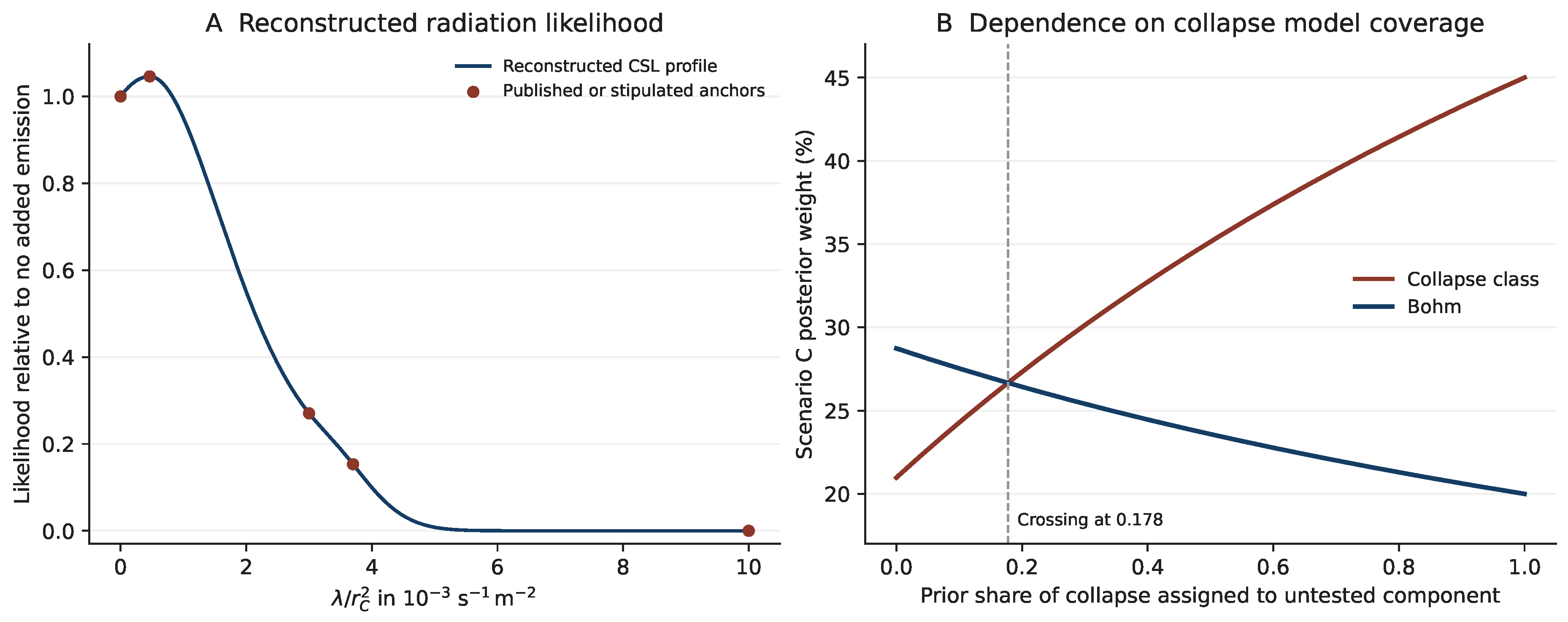
Table 2.
Approximate posterior percentages for scenarios A–H defined in Table 1, using XENONnT and the stated priors, with the specified ten-entry completion. The three marked entries assume unit evidence factors; they have no calculated likelihood in this analysis. The collapse entry is only the equal white-noise CSL/DP benchmark.
Table 2.
Approximate posterior percentages for scenarios A–H defined in Table 1, using XENONnT and the stated priors, with the specified ten-entry completion. The three marked entries assume unit evidence factors; they have no calculated likelihood in this analysis. The collapse entry is only the equal white-noise CSL/DP benchmark.
| Account | A | B | C | D | E | F | G | H |
| Everett | 45.93 | 3.34 | 2.87 | 8.17 | 3.04 | 10.28 | 8.28 | 25.87 |
| Bohm | 15.31 | 50.07 | 28.73 | 5.10 | 2.03 | 15.42 | 10.35 | 25.87 |
| CSL/DP benchmark | 0.99 | 5.42 | 20.98 | 0.99 | 0.66 | 1.33 | 1.68 | 1.68 |
| Relational | 10.21 | 5.56 | 4.31 | 45.93 | 15.21 | 8.22 | 5.17 | 12.42 |
| QBism | 5.10 | 2.23 | 2.87 | 10.21 | 35.48 | 3.08 | 3.10 | 8.28 |
| Consistent histories | 10.21 | 8.90 | 7.18 | 15.31 | 10.14 | 8.22 | 5.17 | 10.35 |
| Operational | 2.04 | 3.34 | 7.18 | 5.10 | 25.34 | 2.06 | 4.14 | 4.14 |
| Retrocausal† | 3.06 | 13.35 | 11.49 | 2.04 | 1.01 | 41.11 | 15.52 | 5.17 |
| Superdeterminism† | 2.04 | 2.23 | 2.87 | 2.04 | 1.01 | 3.08 | 36.22 | 1.03 |
| Other† | 5.10 | 5.56 | 11.49 | 5.10 | 6.08 | 7.19 | 10.35 | 5.17 |
Disclaimer/Publisher’s Note: The statements, opinions and data contained in all publications are solely those of the individual author(s) and contributor(s) and not of MDPI and/or the editor(s). MDPI and/or the editor(s) disclaim responsibility for any injury to people or property resulting from any ideas, methods, instructions or products referred to in the content. |
© 2026 by the authors. Licensee MDPI, Basel, Switzerland. This article is an open access article distributed under the terms and conditions of the Creative Commons Attribution (CC BY) license (http://creativecommons.org/licenses/by/4.0/).
Copyright: This open access article is published under a Creative Commons CC BY 4.0 license, which permit the free download, distribution, and reuse, provided that the author and preprint are cited in any reuse.