

Submitted:
29 September 2026
Posted:
30 September 2026
You are already at the latest version
Abstract
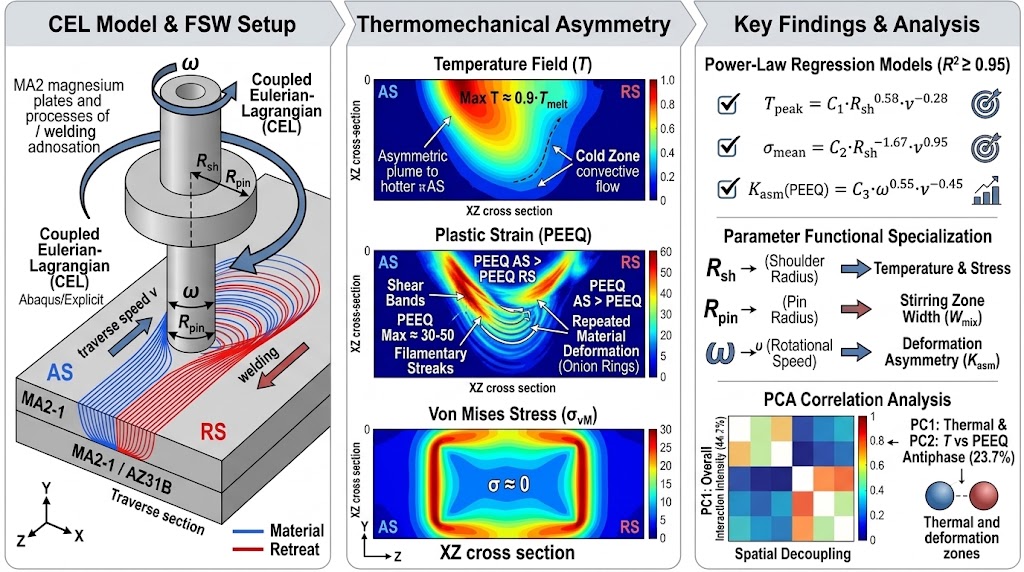
Friction stir welding (FSW) is a promising solid-state joining process for magnesium al-loys that avoids defects characteristic of fusion welding. In the present study, a three-dimensional, fully coupled thermomechanical model of FSW of two 3.0-mm-thick MA2-1 (AZ31B) alloy plates was developed using the Coupled Eulerian–Lagrangian (CEL) approach in Abaqus/Explicit. The constitutive behavior of the material was de-scribed using the Johnson–Cook model (A = 172 MPa, n = 0.456, m = 0.90), while contact interaction was represented by a modified Coulomb–Tresca friction law (μ = 0.40, δ = 0.60). A parametric study of 11 configurations was performed by varying the shoulder diameter R_sh (6–12 mm), pin diameter R_pin (2–4 mm), rotational speed ω (600–1200 rpm), and traverse speed v (60–180 mm/min). A functional specialization of the parame-ters was established: R_sh dominates the thermal regime (exponent +0.58 for T_peak) and the stress state (−1.67 for σ_mean); R_pin controls the width of the stirring zone (W_mix, exponent +0.88); and rotational speed ω is the key factor governing AS/RS deformation asymmetry (K_asm(PEEQ) = 1.10–1.40). Power-law regression equations were obtained for T_peak, σ_mean, PEEQ_max, and W_mix, with R² ≥ 0.95. Spatial correlation analysis confirmed the independence of the thermal and deformation zones, with r(T, PEEQ) = 0.07. Principal component analysis (PCA) identified two dominant mechanisms: a 'com-mon interaction zone' (PC1, 44.7%) and an HAZ–TMAZ antiphase (PC2, 23.7%).
Keywords:
friction stir welding (FSW)
; MA2-1 magnesium alloy (AZ31B)
; CEL modeling
; Abaqus/Explicit
; thermomechanical asymmetry
; Johnson–Cook model
; PEEQ
; regression equations
1. Introduction
1.1. Lightweight Alloys in Modern Structures and the Challenge of Joining Them
Global environmental and energy challenges of the 21st century—including stricter CO₂ emission regulations, rising energy costs, and mandatory fuel-economy standards—have created an urgent need for the widespread use of lightweight structural materials in the aerospace, automotive, shipbuilding, and space-rocket industries. It has been established that a 10% reduction in vehicle mass increases fuel economy by 6–8% [1]. Aluminum (ρ ≈ 2.70 g/cm³) and magnesium (ρ ≈ 1.74 g/cm³) alloys are the principal candidates for replacing steel (ρ ≈ 7.86 g/cm³), enabling structural weight reductions of 40–55% and up to 75%, respectively, while retaining acceptable specific strength characteristics. Magnesium alloys, the lightest structural metallic materials, are used in load-bearing aircraft structures, aircraft interior components, control systems and steering columns, as well as body panels and cladding components of high-speed trains.
However, joining magnesium alloys by conventional fusion-welding methods is associated with fundamental difficulties arising from the physicochemical characteristics of magnesium, including high chemical reactivity and susceptibility to ignition, limited gas solubility in the melt, pore and hot-crack formation during solidification, and embrittlement caused by oxide inclusions. The hexagonal close-packed (HCP) crystal lattice of magnesium results in a limited number of active slip systems at room temperature, restricting ductility and substantially complicating deformation processing during conventional welding operations. Consequently, solid-state joining methods, and particularly friction stir welding (FSW), have acquired major importance over the past decade as a technology capable of producing high-quality magnesium-alloy joints without these limitations [2,3].
Friction stir welding (FSW), developed at The Welding Institute (TWI, UK) in 1991, is a solid-state process in which a rotating tool consisting of a shoulder and a pin travels along the joint, providing localized heating and intense viscoplastic flow of the material without reaching the melting point (Figure 1a).
Compared with arc welding, FSW (Figure 1b,c) eliminates porosity and hot cracking, reduces residual stresses and angular distortions, provides fine dynamically recrystallized equiaxed grains in the stir zone (SZ), and yields joint efficiencies of 85–95% of base metal strength without protective shielding gases or filler wire.
1.2. Need for Numerical Modeling: Physical Limitations of a Purely Experimental Approach
Experimental investigation of FSW encounters several fundamental limitations associated with the extreme thermomechanical conditions in the stirring zone. Temperatures in the pin region reach 0.6–0.9 of the melting temperature (T_melt), strain rates reach 10²–10³ s⁻¹, and accumulated plastic strains exceed 20–100. Direct instrumental measurement of these quantities in real time is technically extremely difficult: thermocouples embedded in the material are destroyed by the tool or disturb the material flow; digital image correlation (DIC) cannot be applied to the enclosed stirring zone; and X-ray tomography requires process interruption and does not provide real-time data. Consequently, most experimental studies are limited to temperature measurements at several points outside the stirring zone, metallographic assessment of weld macrostructure, and mechanical testing, without allowing the complete temperature, strain, and stress fields to be reconstructed directly within the viscoplastic flow region [5].
Numerical modeling overcomes these limitations: a three-dimensional, fully coupled thermomechanical finite-element model provides all field variables throughout the computational domain with arbitrary spatial and temporal resolution. This enables capabilities unavailable experimentally, including visualization of viscoplastic material flow (EVF), calculation of accumulated strain (PE), prediction of defect-initiation zones and voids (VOID, Flash), and evaluation of equivalent residual stresses (MISES) and equivalent plastic strains (PEEQ). Parametric computational studies allow multidimensional process-parameter spaces to be explored within a reasonable time, which is experimentally impractical because of the cost and time required for specimen production [4,6]. A key requirement for reliable numerical results is model verification against experimental data, which provides model “calibration” before predictive use; verification is what transforms a numerical calculation from an illustrative tool into a reliable engineering-design tool.
In this sense, numerical modeling and experiment are not competing approaches but mutually complementary components of a unified research strategy. Experiments provide measurable data for verification, including thermocouple temperature histories, weld macrostructural parameters, hardness profiles, and EBSD maps of grain orientations and sizes. A verified model, in turn, enables experimental observations to be interpreted in terms of mechanical and thermal-field distributions that cannot be measured directly. This “experiment for verification, model for understanding” approach has become a de facto modern standard in FSW research [7,8].
1.3. Numerical Methods for Modeling FSW of Lightweight Alloys (CEL / ALE / SPH / CFD)
Four principal classes of numerical approaches are used to model FSW: (1) Arbitrary Lagrangian–Eulerian (ALE); (2) Coupled Eulerian–Lagrangian (CEL); (3) Smoothed Particle Hydrodynamics (SPH); and (4) Computational Fluid Dynamics (CFD/FVM with a viscoplastic-flow rheological model). Each has fundamental advantages and limitations that differ substantially for magnesium alloys compared with aluminum alloys. The ALE approach, implemented, for example, in Forge 3D [9], provides high accuracy in describing the velocity field in the stirring zone at moderate strains; however, at ω > 800 rpm and high sliding velocities near the pin side surface, Mg alloys exhibit substantially higher flow velocities than Al alloys under the same conditions, leading to catastrophic ALE-mesh distortion and requiring expensive adaptive remeshing with associated accuracy loss [10].
The CEL formulation fundamentally resolves this problem: the material flows through a fixed Eulerian mesh without deforming it, ensuring computational stability at any flow velocity. The tool remains a Lagrangian body, allowing contact interactions to be represented accurately. A comparative study [10] for AZ31B showed that CEL and ALE produce nearly identical temperature and strain fields at ω = 600–1200 rpm, whereas CEL achieves this with a lower mesh density and 1.8–2.3 times shorter computational time—a critical advantage for parametric studies. An additional advantage of CEL is its built-in support for EVF (the material volume fraction in each element), which provides direct visualization of material flow and phase mixing—an option absent from standard ALE packages. For this reason, CEL in Abaqus/Explicit became a preferred tool for CEL-based FSW modeling of Mg alloys during 2019–2025 [11,12,13].
The SPH (Smoothed Particle Hydrodynamics) method is a mesh-free Lagrangian approach that can describe extreme deformations without mesh-related problems. Pan et al. [14] developed an SPH model with non-Newtonian rheology for FSW of a magnesium alloy, demonstrating adequate reproduction of twinning mechanisms and recrystallization zones. Marode et al. [15] used SPH to compare FSW and stationary-shoulder FSW (SSFSW) of AA6061 aluminum alloy. The principal limitations of SPH are its high computational cost (5–10 times greater than CEL for comparable accuracy) and substantial “noise” in pressure and stress fields owing to the stochastic nature of the method. CFD/FVM methods, implemented in FLUENT and OpenFOAM with Herschel–Bulkley or Bingham rheology, provide the most physically realistic description of viscoplastic flow in the “softened” material region; however, they fundamentally cannot represent elastic effects, residual stresses, or defects in the “solid” region outside the stirring zone. For dissimilar Al/Mg material pairs, where differences in thermophysical properties create strong flow asymmetry, a multiphase CFD approach has shown good results [16]. Nevertheless, its applicability is limited to steady-state problems without representation of the heating/cooling cycle. The choice of CEL in the present work was therefore motivated by its optimum balance of accuracy, computational cost, and the ability to describe thermal, deformation, and flow processes within a single coupled framework.
The selection of a constitutive model to describe material rheology under FSW conditions is one of the key methodological decisions determining the reliability of the simulation results. The original Johnson–Cook (JC) model [17], which defines the yield-stress dependence multiplicatively on strain hardening (εⁿ), strain-rate hardening (ln ε̇), and thermal softening (T*/T_melt)ᵐ, offers several practical advantages: a minimal number of parameters (five constants) calibrated using standard dynamic-compression tests (Split Hopkinson Bar); direct compatibility with explicit solvers in Abaqus and LS-DYNA; and a broad literature database of calibrated parameters for aluminum and magnesium alloys. Accordingly, the JC model is the most widely used constitutive model in CEL-based FSW simulations and is employed in most of the studies analyzed [7,10,11]. For MA2-1/AZ31 magnesium alloy, the JC parameters were calibrated by Zhang et al. (2020) accounting for {0002} texture: A = 172 MPa, B = 361 MPa, n = 0.456, C = 0.092, m = 0.90.
The main limitation of the standard JC model for magnesium alloys is its inherent isotropy. The HCP lattice of magnesium exhibits pronounced crystallographic anisotropy, and at temperatures below 200 °C the dominant deformation mechanism is {10-12} extension twinning rather than slip. The JC model accounts for neither the anisotropy of the initial yield stress nor twinning or dynamic recrystallization (DRX). According to Zhang et al. [18], at T = 293 K and ε̇ = 10³ s⁻¹, the standard JC model underestimates σ_y for AZ31 in the ND direction by 15–20% because of the contribution of twinning. The authors proposed a modified temperature term, replacing the standard polynomial with an exponential form, which reduced the average absolute relative error (AARE) from 12.8% to 4.7% over the temperature range 20–350 °C. Nevertheless, within the high-temperature FSW range (400–650 °C), where twinning is suppressed, the standard JC model provides sufficient accuracy for engineering calculations.
The Zerilli–Armstrong model [19] accounts for the physics of dislocation slip through different dependencies of the yield stress σ_y on T and ε̇ for FCC (Al) and BCC (steel) crystal lattices. An extended ZA formulation exists for HCP materials (Mg, Ti) that includes terms for slip and twinning. Comparative analysis by Serindag and Kiral [20] showed that the modified ZA model (MZA) provides slightly higher accuracy in predicting the yield stress σ_y of AZ31B at 50–250 °C (R² = 0.9946 versus 0.9945 for the modified JC model), but it requires twice as many constants (10 versus 5) and has no direct implementation in the standard Abaqus libraries.
The Arrhenius–Zener–Hollomon model (hyperbolic-sine equation), widely used in hot-deformation modeling, provides the highest accuracy (R² > 0.999) over narrow ranges of temperature T and strain rate ε̇ typical of hot rolling or forging. However, it loses its universality when broad ranges of T (20–650 °C) and ε̇ (10⁻³–10³ s⁻¹), characteristic of FSW, are considered simultaneously.
Neural networks and Gaussian Process Regression (GPR) provide maximum flexibility but lack direct physical interpretability and require extensive experimental databases for the alloys being modeled. The JC model was therefore selected in the present work because of its adequate accuracy in the high-temperature FSW regime, practical implementation, and availability of verified parameters for MA2-1/AZ31 alloy.
1.4. CEL Modeling of FSW: Alloys, Results, and Comparison
Over the past 5–7 years, the CEL method (Coupled Eulerian–Lagrangian) has become one of the leading numerical approaches for FSW modeling. In 2018, Nezamdost et al. [21] applied CEL in Abaqus/Explicit to FSW of AA5083 aluminum alloy and showed that the CEL model reproduced experimental temperature histories with an error of no more than 8%, while avoiding the mesh-distortion problems characteristic of purely Lagrangian models. Turkan and Karakaş [10] directly compared CEL and ALE for joining wrought AZ31B magnesium alloy during the tool-plunge stage. Both approaches produced similar temperature and strain fields; however, ALE required a substantially higher mesh density in the contact region to avoid divergence, whereas CEL remained stable at the same density up to ω = 1200 rpm. This study became a key benchmark for CEL modeling of Mg-alloy FSW and is widely cited as evidence supporting the preference for CEL in magnesium systems.
In 2021–2022, a number of studies extended CEL beyond conventional aluminum alloys. Bîrsan and Bașliu [22] applied CEL in Abaqus to refill friction stir spot welding (RFSSW) of high-strength wrought aluminum alloys 6061-T6 and 5052-H321, demonstrating the ability to model keyhole closure and phase mixing at different rotational speeds, with a calculated peak weld-zone temperature of ~670 K. In the same period, the CEL approach was applied to FSW of a magnesium alloy in a study of Bobbin Tool capabilities [23]. The simulations showed that, in the shoulder region, material moves from AS toward RS, whereas in the pin region the direction is reversed. This complex asymmetric double-flow pattern was reproduced by the CEL model but was not captured by simplified physical thermal models. Iordache et al. [13] used CEL in Abaqus 2021 to model FSW of structural wrought AA6082-T6 aluminum alloy (Al-Mg-Si-Mn system) with detailed treatment of boundary conditions and tool geometry; the error in predicted stirring-zone width was no more than 2.5%.
In 2023–2024, the application of CEL modeling expanded substantially. Zhang et al. [24] developed a CEL model to investigate residual stresses in FSW of AA6061-T6 wrought aluminum alloy and confirmed the characteristic M-shaped asymmetric distribution of longitudinal residual stresses. Peak tensile stresses on AS (~170 MPa) exceeded those on RS (~150 MPa). Feng et al. [11] implemented an analytical CEL model for FSW of AZ31 magnesium alloy, with parameters calibrated against high-temperature tensile curves. The predicted temperature fields agreed well with thermocouple measurements, with an error of ~6%. Wang et al. [12] applied CEL to investigate the effect of pin taper angle in the thermomechanically affected zone (TMAZ) during FSW of aluminum alloys and found that increasing the taper angle from 0° to 60° broadened the longitudinal thermal gradient and reduced the material-flow velocity near the pin tip. Finally, Behnagh et al. [25] used a two-step CEL model to predict processing temperature and grain size during friction stir processing of magnesium chips, demonstrating the applicability of CEL beyond sheet welding.
Analysis of published CEL studies reveals several common trends. First, all authors note that the CEL method in Abaqus/Explicit maintains computational stability at high rotational speeds ω and traverse speeds v without the element inversion problems typical of Lagrangian approaches. Second, temperature-field prediction errors are generally 5–10% relative to thermocouple data when the friction coefficient μ and plastic-dissipation coefficient η are selected appropriately. Third, CEL models provide a unique capability for quantitatively describing material flow (EVF) and phase mixing, which is unavailable in both ALE and thermal FEM models. This latter feature makes CEL particularly valuable for investigating AS/RS thermomechanical asymmetry and predicting defects such as tunnel voids and insufficient penetration. At the same time, publications on CEL modeling of FSW in magnesium alloys, especially those involving systematic parametric analysis of tool geometry effects on asymmetry, remain limited; the present study is intended to address this gap.
1.5. Thermomechanical Asymmetry between AS and RS: Mechanisms and Physical Origin
Thermomechanical asymmetry between the Advancing Side (AS) and Retreating Side (RS) of a weld is one of the fundamental characteristics of the FSW process, with a decisive influence on weld quality, microstructural-zone distribution, and joint mechanical properties. The physical origin of this asymmetry is determined by the kinematics of tool motion: the velocity of any point on the pin or shoulder surface in the laboratory reference frame is the superposition of a rotational component (ω·r, tangential) and a translational component (v_weld, along the welding direction). On the AS, these components add in the region of maximum approach to the leading wall of the stirring zone, giving the resultant sliding velocity v_slip_AS = ω·r + v_weld, whereas on the RS they subtract, v_slip_RS = |ω·r − v_weld|. For typical FSW parameters (ω = 800 rpm, R_sh = 9 mm, v_weld = 100 mm/min ≈ 1.67 mm/s), v_slip_AS = 13.3·9 + 1.67 ≈ 121 mm/s and v_slip_RS ≈ 118 mm/s; the difference is ~2.8%, which appears small. However, the nonlinear dependence of frictional heat generation q_fric on sliding velocity (q_fric ∝ μ·p·v_slip²) amplifies this difference and produces a persistent temperature differential ΔT in favor of AS.
The asymmetry in heat generation initiates a chain of coupled consequences. The higher temperature on AS produces more pronounced thermal softening, reducing the yield stress σ_y and thereby facilitating material capture and transport by the rotating tool. This results in asymmetric material flow (EVF): on AS, material is captured more effectively by the tool and transported into the stirring zone in larger volumes per revolution. On RS, in contrast, part of the material remains in the peripheral region and is not incorporated into intense mixing, creating a risk of tunnel-defect formation under insufficient heat input [26,27]. The asymmetry in accumulated plastic strain (PEEQ) is a direct consequence of the different numbers of material passages through the tool-contact region: on AS, each elementary material volume passes through the high-shear zone more times per unit weld length than on RS, producing a monotonic increase in K_asm(PEEQ) with increasing weld length.
AS/RS asymmetry in FSW of dissimilar material pairs (Al/Mg, Al/Ti) is especially pronounced and qualitatively changes the flow pattern. For example, CFD modeling of dissimilar Al/Ti FSW [28] showed that, near the shoulder, the temperature on the titanium side (Ti, AS) is higher than on the aluminum side (Al, RS), consistent with the higher yield stress and lower thermal conductivity of titanium; farther from the shoulder, however, the pattern reverses. In such a pair, more than 80% of the plastic flow is concentrated on the aluminum side (RS) because aluminum has substantially lower viscosity at FSW temperatures. For homogeneous Mg/Mg joints, by contrast, the flow is more symmetric, although PEEQ and EVF asymmetry persists. These trends strongly indicate that the mechanism of AS/RS asymmetry is common to FSW systems, while its quantitative characteristics are determined by the rheological and thermophysical properties of the specific material.
Quantitative data on thermomechanical field asymmetry in magnesium alloy FSW vary substantially with welding parameters, tool geometry, experimental configuration, and numerical model. For homogeneous AZ31/AZ31 pairs at ω = 600–1200 rpm and v = 60–200 mm/min, the typical temperature difference ΔT between AS and RS, measured by thermocouples 5 mm from the weld centerline, is approximately 15–35 °C; at a mean weld temperature of ~450–550 °C, this corresponds to a relative asymmetry of ~3–7%. Peak temperatures immediately adjacent to the pin surface are estimated by numerical models at 500–650 °C (0.84–0.98 of the AZ31 melting temperature). Values above 0.95 T_melt generally indicate an overestimated friction coefficient or insufficient accounting for heat dissipation into the backing plate [10,11,29].
Plastic-strain asymmetry in magnesium-alloy FSW is considerably stronger than thermal asymmetry. In the CEL modeling study of AZ31B by Turkan and Karakaş [10], PEEQ_max on AS was approximately 20–30% higher than on RS at ω = 800 rpm and v = 100 mm/min. Increasing ω to 1200 rpm increased the difference to 35–45%. In studies of dissimilar Al/Mg FSW, the quantitative asymmetry is substantially stronger. During welding of a magnesium alloy, the EVF-based fraction of Mg material incorporated into mixing on AS exceeds the fraction of Al material on RS by 15–25% of the weld cross-sectional area. These data are consistent with the view that the higher viscosity of magnesium than aluminum at FSW temperatures (due to the higher T_melt) reduces convective mixing intensity, making the Mg side more resistant to material mixing. For analogous homogeneous Al/Al joints, thermal asymmetry ΔT at 5 mm from the centerline reaches ~20 °C at ω = 800 rpm [7,27], which is comparable with the data for magnesium alloys.
Typical temperature ranges during FSW differ substantially among alloys. For Al alloys (6061-T6, 2219-T87), peak weld-zone temperatures are 400–550 °C (0.70–0.90 T_melt); for Mg alloys (AZ31, MA2-1), 450–650 °C (0.84–0.98 T_melt); for Ti-6Al-4V, 700–850 °C (0.55–0.67 T_melt); and for steels, 1000–1200 °C (0.65–0.78 T_melt). Peak equivalent plastic strains, PEEQ_max, during the steady FSW stage are determined by the residence time of material in the high-shear zone and by rotational speed. For Al alloys, PEEQ_max is ~30–60 in the tool wake, whereas for Mg alloys it is 30–50 under comparable welding conditions. Maximum strain rates ε̇_max near the pin side surface reach 500–2000 s⁻¹ for aluminum alloys and 300–800 s⁻¹ for magnesium alloys at ω = 800 rpm. This difference is attributed to the higher viscosity of Mg, which limits the shear rate.
1.6. Parametric Studies of Tool Geometry and FSW Conditions: Effects on Asymmetry and Defect Formation
The geometric parameters of an FSW tool—the shoulder diameter and profile (R_sh), pin shape, diameter and length (R_pin, L_pin), and taper angle—together with the process parameters ω and v form a multidimensional factor space governing heat input, material-flow behavior, asymmetry, and defect probability. Experimental studies have shown that, at a fixed R_sh/R_pin ratio of approximately 3 (a commonly used ratio for Al and Mg alloys) and ω/v = 8–12 rev/mm (tool pitch), defect-free welds can be obtained. Exceeding these limits leads either to excessive heat generation and Flash (high ω, low v, large R_sh) or to tunnel-type VOID defects (low ω, high v, small R_pin). For AZ31B with plate thicknesses of 4–6 mm, optimal ranges of rotational and traverse speeds of ω = 600–1200 rpm and v = 60–200 mm/min have been reported [29,30].
With respect to AS/RS asymmetry, CEL- and ALE-based parametric studies have established the following trends. The effect of rotational speed ω on PEEQ asymmetry is dominant. Increasing ω at constant v increases the sliding-velocity difference v_slip_AS − v_slip_RS = 2·v_weld (which is independent of ω), while increasing the ratio ω·r/v_weld, which determines the relative contribution of asymmetry to the overall flow. At ω = 1200 rpm, K_asm(PEEQ) is 20–25% higher than at ω = 600 rpm at the same traverse speed v. The effect of shoulder size R_sh on heat-generation asymmetry is also significant: a larger shoulder produces a larger peripheral contact area, where the difference v_slip_AS − v_slip_RS is most pronounced. The effect of pin size R_pin on K_asm(PEEQ) is minimal; however, the pin is the key parameter controlling stirring-zone width, W_mix ∝ R_pin_bot. Tunnel defects in magnesium-alloy FSW are primarily associated with insufficient heat input (small R_sh or ω) and/or high v, which do not provide adequate preheating before pin capture. Flash forms under excessive heat input and insufficient shoulder pressure, corresponding to large R_sh and low traverse speed v [3,31].
The influence of pin profile on asymmetry and defect formation was investigated using CEL in a study of a Triflute FSW tool [32]. The three-lobed pin generates a pulsating flow pattern with periodic high-stress zones around each lobe; this increases overall heat generation and reduces susceptibility to tunnel defects compared with a smooth conical pin, but simultaneously increases PEEQ asymmetry by 10–15% because of the loss of axial flow symmetry. Similar results were obtained for square, triangular, and hexagonal pins in CEL simulations of Bobbin Tool FSW of a magnesium alloy [23]. For non-cylindrical pins, periodic interaction with the faces enhances convective mixing but creates local strain concentrations shifted toward AS. These results emphasize that pin-profile selection is an important means of controlling asymmetry alongside the welding-speed parameters.
1.7. Experimental Verification of CEL Models: Methods and Levels of Reliability
CEL models of FSW are verified at several levels that differ in information content and accessibility. The most common method is thermal verification using thermocouple data (K-type, chromel–alumel) obtained from holes positioned 5–20 mm from the weld centerline at fixed depths. In most verified CEL studies, the discrepancy between simulated and experimental temperature histories is 5–12% in peak value and 8–15% in cooling-curve shape. Refined CEL models with temperature-dependent friction μ(T) and contact thermal resistance reduce the error to 3–6% [7,11,13]. Importantly, thermal verification does not guarantee model accuracy in the immediate stirring zone near the pin because thermocouples in this region are destroyed by the tool.
A more informative method is geometric verification based on the width of the stirring zone (SZ) and thermomechanically affected zone (TMAZ) observed in metallographic cross-sections. The SZ width is defined as the region where EVF ∈ (0.1, 0.9) and is compared with the region in which the original-material traces disappear after metallographic etching. In the study by Iordache et al. [13] for AA6082 FSW, this comparison gave an SZ-width error of 2.5% and a stirring-zone penetration-depth error of 4.1%. For magnesium alloys, such verification is complicated by weaker etching contrast and by the difficulty of identifying TMAZ/HAZ boundaries. A promising addition is electron backscatter diffraction (EBSD), in which grain-orientation maps can be directly compared with predicted high-deformation zones (PEEQ > 2–5 as an indicator of DRX). Finally, verification based on tool reaction forces (axial force F_z, torque M, transverse force F_y) is both quantitative and integral, combining the accuracy of the contact conditions, rheology, and heat-transfer description. For aluminum alloys, the error of CEL predictions for F_z is typically 8–15%; corresponding literature data for magnesium alloys are limited [10].
Analysis of the literature reveals several gaps in understanding FSW of magnesium alloys within the CEL framework. First, most CEL studies of magnesium alloys [10,11,25] are limited either to a single process stage (plunging) or to a single parameter set and do not conduct systematic parametric analysis of R_sh, R_pin, ω, and v simultaneously. Second, a quantitative characterization of AS/RS asymmetry through the dimensionless coefficients K_asm(T), K_asm(PEEQ), and K_asm(σ), together with the evolution of time histories for magnesium alloys in the CEL formulation, is absent from the literature. Third, spatial statistical analysis (Pearson correlation and PCA) of thermomechanical fields during the steady FSW stage has not previously been applied to either magnesium or aluminum systems in the context of CEL modeling. The present work addresses these gaps by providing an extended parametric CEL study of FSW of 3.0-mm-thick MA2-1 plates, including the full set of thermomechanical fields, their temporal evolution, quantitative AS/RS asymmetry, and statistical analysis of their interrelationships.
The objective of the present study is to numerically investigate the characteristics of thermomechanical asymmetry arising during FSW of two MA2-1 magnesium-alloy plates and to analyze the effects of tool geometric parameters (shoulder diameter R_sh and pin diameter R_pin) and process conditions (rotational speed ω and traverse speed v) on the spatial distributions of temperature, equivalent plastic strain (PEEQ), equivalent von Mises stress (MISES), material flow (EVF), and mixing index in the XZ plane of the weld cross-section.
The main objectives of the present study are:
- Develop a three-dimensional, fully coupled thermomechanical CEL model of FSW of MA2-1 plates in Abaqus/Explicit.
- Select and justify the Johnson–Cook constitutive model with complete mathematical description for MA2-1 alloy.
- Verify the model by comparing calculated temperature fields with literature and experimental data for AZ31/MA2-1 alloys.
- Analyze the time histories and steady-state behavior of maximum and mean temperature, stresses, PEEQ, and mixing index.
- Quantitatively characterize AS/RS thermomechanical asymmetry during FSW using K_asm and evaluate parameter sensitivity.
- Perform statistical analysis of results, including spatial correlations and PCA of thermomechanical fields, deriving predictive power-law regression equations.
2. Materials and Modeling Methodology
2.1. Material: MA2-1 Alloy
The material investigated was the wrought magnesium alloy MA2-1 (GOST 14957-76), whose chemical composition corresponds to the international AZ31B grade: Mg—balance, Al 2.5–3.5%, Zn 0.6–1.4%, and Mn 0.2–0.5% (wt.%). The alloy density is 1780 kg/m³, making it one of the lightest structural metallic alloys. The hexagonal close-packed (HCP) crystal lattice gives the alloy distinctive deformation behavior. At temperatures below 200 °C, twinning on {10-12} planes and dislocation slip on basal planes dominate, whereas above 300 °C additional non-prismatic and pyramidal slip systems become active, and above 400 °C dynamic recrystallization occurs. Within the FSW temperature range (400–650 °C), MA2-1 behaves as an isotropic viscoplastic material, justifying the use of an isotropic Johnson–Cook (JC) constitutive model. Thermophysical properties were assumed constant, which is a standard assumption in CEL simulations of FSW [10]. The principal properties of MA2-1 are listed in Table 1.
2.2. Governing Equations of the CEL Model
Within the CEL formulation, the conservation equations of mass, momentum, and energy are solved simultaneously at each material point in the Eulerian mesh in a form appropriate for incompressible, thermally activated viscoplastic flow. The complete system of differential equations used by the Abaqus/Explicit solver is presented below, together with the role of each term and the point at which the Johnson–Cook model enters the formulation.
Continuity equation (mass conservation). For an incompressible viscoplastic material in the Eulerian reference frame, the mass-conservation equation is:
where ρ is the density [kg/m³]; t is time [s]; v is the material-flow velocity vector [m/s]; and ∇· is the divergence operator. Material incompressibility is additionally assumed: ∇·v ≈ 0. In the CEL formulation, this equation governs the change in the material volume fraction EVF in each Eulerian element, enabling accurate tracking of material flow without mesh degradation
∂ρ/∂t + ∇·(ρv) = 0
Equation of motion (momentum conservation). The differential form of the momentum-conservation equation for a viscoplastic body is:
where σ is the Cauchy stress tensor [Pa] and g is the gravitational acceleration vector [m/s²] (g = 0 is assumed). The left-hand side represents inertial terms, whereas the right-hand side represents the divergence of the stress field. In Abaqus/Explicit, Equation (2.2) is integrated using an explicit central-difference scheme:
where M is the diagonal mass matrix; F^ext is the external-force vector arising from contact interaction with the tool; F^int is the internal-force vector (the volume integral of σ over the element); and Δt is the integration time step (determined by the CFL condition). The explicit scheme does not require the solution of a system of linear algebraic equations, providing high computational efficiency.
ρ(∂v/∂t + (v·∇)v) = ∇·σ + ρg
v^(i+1/2) = v^(i−1/2) + Δt M⁻¹·(F^ext − F^int)
Energy equation (heat conduction with heat sources). The transient heat-conduction equation with convective heat transport and volumetric heat sources is:
where cₚ is the specific heat capacity [J/(kg·K)]; T is temperature [K]; λ is thermal conductivity [W/(m·K)]; the term v·∇T represents convective heat transport by the viscoplastic flow (a specific contribution of the CEL formulation absent from Lagrangian models); Q_plast is the volumetric heat source due to plastic dissipation [W/m³]; and Q_fric is the surface heat source due to friction [W/m²], prescribed as a boundary condition at the contact surface. Equation (2.4) provides the thermodynamic coupling between mechanics (through Q_plast and v) and the temperature fields.
ρcₚ(∂T/∂t + v·∇T) = ∇·(λ∇T) + Q_plast + Q_fric
Strain decomposition and plasticity criterion. The total strain-rate tensor is decomposed into elastic and plastic components:
ε̇ᵢⱼ = ε̇ᵉᵢⱼ + ε̇ᵖᵢ
The elastic component is described by Hooke’s law with thermal expansion:
where Cijkl is the fourth-order tensor of elastic moduli; α is the coefficient of thermal expansion; and δkl is the Kronecker delta. The plasticity criterion is formulated using the von Mises invariant:
where σvM = √(3sᵢⱼsᵢⱼ/2) is the von Mises stress and sᵢⱼ = σᵢⱼ − (σₖₖ/3)δᵢⱼ is the deviatoric stress tensor. The yield condition (2.7) receives σy from the Johnson–Cook model; this is the point at which the JC model enters the governing-equation system. Plastic flow is described by the associated normality rule:
where λ̇ is the scalar plastic multiplier determined from the consistency condition ḟ = 0
σ̇ᵢⱼ = Cᵢⱼₖₗ(ε̇ᵉₖₗ − α Ṫ δₖₗ)
f = σvM − σy(εₚ, ε̇, T) = 0
ε̇ᵖᵢⱼ = λ̇ ∂f/∂σᵢⱼ = λ̇ (3/2) sᵢⱼ/σvM
2.3. Johnson–Cook Constitutive Model and Heat-Generation Equations
To describe the elastic–viscoplastic behavior of MA2-1 at the high temperatures, strain rates, and accumulated strains characteristic of FSW, the Johnson–Cook model [17] is employed in multiplicative form
where the dimensionless homologous temperature T* is defined as:
where σy is the yield stress (MPa); A = 172 MPa is the quasi-static yield stress at T_ref; B = 361 MPa is the strain-hardening coefficient; n = 0.456 is the hardening exponent; C = 0.092 is the strain-rate hardening coefficient; m = 0.90 is the thermal-softening exponent; εp is the accumulated plastic strain; ε̇* = ε̇/ε̇₀ is the normalized strain rate; T_ref = 293 K; T_melt = 923 K.
σy = (A + B·εₚⁿ) (1 + C·ln(ε̇/ε̇₀)) [1 − T*ᵐ]
T* = (T − T_ref) / (T_melt − T_ref), T* ∈ [0,1]
Parameters A, B, and n describe strain hardening under quasi-static loading; the second term describes logarithmic strain-rate hardening; the third multiplier represents thermal softening and approaches zero as T → T_melt. The parameters were calibrated against the data of Zhang et al. [18] for AZ31 with {0002} texture and are applicable to MA2-1 over T = 200–600 °C.
The accumulated plastic strain (PEEQ) is determined by integrating the plastic-strain rate:
where ṗ is the equivalent plastic-strain rate [s⁻¹]. PEEQ is a monotonically increasing scalar representing the complete “history” of plastic deformation of a given material volume. It is the principal field variable characterizing the intensity of tool-induced deformation and is used in the present work to quantify AS/RS asymmetry.
Total heat generation in the model consists of two contributions. The frictional component at the tool–material contact surface is described by a modified Coulomb law limited by the Tresca criterion:
where μ = 0.4 is the friction coefficient; p is the normal pressure; and δ = 0.6 is the stick–slip coefficient. The dissipation power per unit area is q_fric = τ_contact v_slip, where v_slip is the sliding velocity of the material relative to the tool. The plastic contribution to volumetric heat generation is
where η = 0.9 is the plastic dissipation coefficient (inelastic heat fraction). The total heat generation in the contact region is Qtotal = Qfric + Qplast. Heat input from the shoulder accounts for Qshoulder/Qtotal ≈ 78–82% under the baseline FSW conditions; this contribution is implemented in the model and agrees with the data of Memon et al. [7].
τ_contact = min(μ p, τlim), τ_lim = δ σy / √3
Q_plast = η_p σ : ε̇ᵖ = η_p σ_vM ε̇_p
2.4. Initial and Boundary Conditions
Initial temperature throughout the workpiece was set to T₀ = 20 °C (293.15 K). Convective and radiative heat dissipation to the environment and conductive losses to the steel backing plate summarized in Table 2.
2.5. AS/RS Velocity Kinematics
The local relative velocity vector v_rel at the tool–workpiece interface is governed by the superposition of rotation and traverse motion. The sliding velocity of the material along the pin side surface at a distance r from the tool axis is given by Equation (2.14):
v_AS = ω·r + v_weld v_RS = ω·r—v_weld
The velocity difference Δv = v_AS − v_RS = 2·v_weld increases with v_weld and is independent of ω; however, the relative asymmetry (ΔT/T_RS) is governed by the ratio ω·r/v_weld. Computational stability is ensured by the automatically selected time increment according to the CFL criterion, Δt ≤ L_min/c, where c is the speed of sound in the material (~5100 m/s for Mg).
2.6. Definition of EVF, Mixing Index, and Asymmetry Coefficient
In the CEL formulation, each Eulerian element is characterized by the volume fraction of each material phase. Material transport is monitored using the Eulerian Volume Fraction (EVF) and the normalized Mixing Index (MI):
where MI = 0 corresponds to pure material and MI = 1 to ideal mixing (0.5/0.5). The dimensionless asymmetry coefficient is defined by (2.16):
EVF = V_mat / V_elem, EVF ∈ [0,1] MI = 1 − |2·EVF_R − 1|, MI ∈ [0.1]
K_asm(Q) = Q_AS / Q_RS
where Q_AS and Q_RS are the integral values of the characteristic under consideration (T, PEEQ, σ_Mises) within ±15 mm of the tool axis, on the AS and RS, respectively, integrated over the full plate thickness in the transverse cross-section during the steady stage (t ≥ 5 s).
2.7. Model Geometry and Computational Parameters
Eulerian domain (stirring zone). Domain dimensions: 60 mm × 150 mm × 5.5 mm (X × Y × Z; an additional 2.5 mm in Z provides a buffer above the plate surface for material expelled as Flash; see Table 3). Element type: EC3D8RT—an 8-node thermally coupled Eulerian hexahedral element with reduced integration (one Gauss point) and enhanced hourglass control (k_hg = 0.05). The letter “T” denotes the coupled thermomechanical formulation, while “R” denotes reduced integration.
Lagrangian side domains. Domain geometry: 2 × (25 mm × 150 mm × 5.5 mm). Element type: C3D8RT—an 8-node thermally coupled Lagrangian hexahedral element with reduced integration. Mesh size: 1.0–3.0 mm, with graded refinement toward the Eulerian domain. Number of elements: ~80.000 in each side domain. The interface with the Eulerian domain is treated by the Eulerian–Lagrangian interface algorithm through kinematic constraints.
Tool domain (Discrete Rigid). The tool is modeled as a perfectly rigid body (Discrete Rigid). Conical pin: root radius R_pin_bot, tip radius R_pin_top = R_pin_bot − 1 mm, length 5.1 mm. Flat shoulder: radius R_sh. The parameter ranges are given in Table 4. Element type: R3D3 (3-node rigid triangle). Number of elements: ~2400 (shoulder) + ~1800 (pin) = ~4200. Rigid-tool behavior is a standard assumption in CEL FSW modeling and is justified by the substantially higher yield stress of the tool material (σy ≈ 900 MPa for H13) compared with MA2-1 at FSW temperatures (~20–150 MPa). Computational resources and parametric-simulation settings are listed in Table 5.
3. Simulation Results
3.1. Parametric Study of CEL Modeling of FSW of MA2-1 Plates
This section presents a systematic analysis of CEL simulation results for FSW of MA2-1 plates for 11 computational configurations covering the parametric design in Table 4: shoulder diameter R_sh (6, 9, 12 mm), pin-base diameter R_pin_bot (2, 3, 4 mm), rotational speed ω (600, 800, 1000, 1200 rpm), and traverse speed v (60, 100, 140, 180 mm/min), with all other parameters fixed (baseline configuration: ω = 800 rpm, R_sh = 9 mm, R_pin = 3 mm, v = 100 mm/min). Each parameter was varied according to the “one factor at a time” (OFAT) principle, allowing its contribution to changes in the weld output characteristics to be isolated and quantified.
The objective of the parametric study is to establish quantitative relationships between the geometric and kinematic FSW parameters and four key weld characteristics: (1) peak temperature T_peak in the stirring zone; (2) mean von Mises stress σ_mean during the steady stage; (3) maximum accumulated plastic strain PEEQ_max; and (4) stirring-zone width W_mix. These four characteristics determine weld quality, microstructure, susceptibility to defect formation, and joint mechanical properties [4,33]. Identifying which parameter controls each characteristic is essential for developing an optimized process window for magnesium-alloy FSW.
The results are analyzed according to the following scheme. First, time histories of all four characteristics are examined for each parameter group (Figure 1 and Figure 2), allowing the evolution of the fields from the plunge stage to the steady regime and comparisons among configurations to be tracked. Next, histograms are constructed for all 11 configurations using steady-state values (t > 4.5 s) (Figure 4), and power-law regression analysis is performed (Figure 5) to obtain compact analytical equations relating welding parameters to the output characteristics.
Figure 2 presents the time histories of maximum and mean temperature (left axis) and maximum von Mises stress (right axis) for all 11 computational configurations, grouped by the varied parameter. The baseline configuration (gray line) is identical in all four plots (Figure 2a–d) and serves as the reference curve for comparison. Three distinct stages are visible in all curves, as described in Section 1.4: Stage I—plunging (t < 0.2 s), with a sharp rise in T_max; Stage II—transitional (0.2 < t < 1.5 s), with decaying oscillations; and Stage III—steady (t > 3 s), with quasi-stationary values. Mean values over Stage III (t = 4.5–10.0 s) are used for the analysis.
Analysis of the effect of shoulder size R_sh clearly demonstrates its dominant influence on the thermal field (Figure 1a). At R_sh = 6 mm, the peak temperature is ~379 °C, 21% below the baseline value (480 °C). At R_sh = 12 mm, the temperature reaches ~567 °C (+18% relative to the baseline), corresponding to 0.93 T_melt and approaching the onset of partial melting along magnesium-alloy grain boundaries. The shoulder accounts for 78–82% of the total heat input (Section 2.3), explaining the strong temperature sensitivity to R_sh. Von Mises stress behaves in the opposite manner: at R_sh = 6 mm, σ_mean ≈ 124 MPa (+61% relative to the baseline 77 MPa) because of insufficient thermal heating, whereas at R_sh = 12 mm, σ_mean decreases to ~37 MPa (−52%) because the weld material is strongly softened by heating to a high temperature. Thus, R_sh is the key parameter controlling the welding thermal regime, and its selection should provide a peak weld-zone temperature of 0.75–0.90 T_melt (420–560 °C for MA2-1).
The simulation results for tool (pin) angular velocity ω (Figure 2b) show a monotonic increase in T_peak with rotational speed, from 425 °C at ω = 600 rpm to 569 °C at ω = 1200 rpm. The exponent is +0.42, meaning that doubling ω increases T_peak by approximately 34%. Physically, this is explained by the increase in sliding velocity at the shoulder periphery, since v_slip ∝ ω·R_sh; therefore, heat generation (q_fric = τ_c·v_slip) increases with rotational speed. Von Mises stress decreases with increasing ω (from ~99 MPa at ω = 600 rpm to ~38 MPa at ω = 1200 rpm), directly reflecting thermal softening in the JC model: at T_peak = 569 °C (T* ≈ 0.80), the yield stress decreases to ~27% of its quasi-static value. The time-history shape also changes: at high ω, Stage I becomes substantially more intense (higher T_max during plunging), but the transition to the steady stage occurs faster.
The effect of traverse speed v on temperature (Figure 2c) is opposite to that of rotational speed ω. At v = 60 mm/min, the peak weld temperature T_peak reaches 554 °C, whereas at v = 180 mm/min it decreases to 407 °C. The exponent has a magnitude of 0.28, so tripling v reduces T_peak by approximately 25%. This is explained by the reduction in heat input per unit weld length (Q/l ∝ Q_total/v). At high traverse speed (180 mm/min), the tool spends less time over each location, reducing material heating and increasing the temperature gradient. Accordingly, von Mises stresses at v = 180 mm/min reach ~116 MPa, the highest value among the speed-variation configurations, creating a risk of insufficient mixing and tunnel defects. At v = 60 mm/min, σ_mean = 41.5 MPa; however, excessive heat input may cause expulsion of part of the weld metal (Flash) and surface oxidation.
Analysis of the fourth parameter, pin diameter, shows that it has the smallest influence on temperature (exponent +0.050). At R_pin = 2 mm, T_peak is 470 °C, whereas at R_pin = 4 mm it increases to 487 °C (+17 °C), corresponding to only a 3.5% increase. This result is expected because the pin contributes only ~18–22% of the total heat input and has a small contribution to the total contact area compared with the shoulder. Mean von Mises stress also changes only slightly, from 81 MPa at R_pin = 2 mm to 74 MPa at R_pin = 4 mm. As shown in Figure 2d, the curves for the two cases are practically indistinguishable, confirming the small contribution of R_pin to the thermal and stress regimes. Physically, this means that the pin acts primarily as a mechanical “stirrer” rather than as a heat source.
3.2. Evolution of Plastic Strain and Stirring-Zone Width
The evolution with time of maximum and mean plastic strain PEEQ (left axis) and stirring-zone width W_mix (right axis) is shown in Figure 3. Unlike temperature and stress, PEEQ does not reach a stationary value because it continues to accumulate monotonically throughout the simulation, as each pin revolution adds deformation to the material in the contact zone. The PEEQ accumulation rate gradually decreases as material migrates away from the region of maximum shear, but it does not reach zero within the simulated time. This is a fundamental difference from temperature, which stabilizes during Stage III.
Analysis of the shoulder-size effect (Figure 3a) shows nearly coincident PEEQ_max curves for all three values (R_sh = 6, 9, 12 mm), with the R_sh exponent equal to zero; thus, shoulder diameter does not affect accumulated strain in the pin region. This can be explained by the fact that PEEQ is governed by shear mechanics at the pin side surface rather than by shoulder heat input. In contrast, W_mix increases slightly with R_sh through the indirect thermal effect, because greater heat input increases the plastified-zone size.
The effect of pin rotational speed ω on the plastic-strain parameters (Figure 3b) produces the largest spread in the PEEQ curves. At the highest simulated speed, ω = 1200 rpm, PEEQ_max ≈ 184, which is 46% higher than at ω = 600 rpm (~126). Rotational speed is therefore the primary control parameter for PEEQ: more revolutions per unit time produce more encounters between the material and the pin surface and hence greater accumulated deformation. W_mix also increases with ω, from 4.5 mm at ω = 600 rpm to 5.8 mm at ω = 1200 rpm (+29%).
The effect of traverse speed v on PEEQ (Figure 3c) is opposite to that of rotational speed ω. At v = 60 mm/min, PEEQ_max = 185 because the tool moves slowly and the material remains longer in the stirring zone, whereas at v = 180 mm/min it decreases to 113. W_mix decreases with increasing v, from 5.7 mm at v = 60 mm/min to 4.3 mm at v = 180 mm/min, because less material is entrained per pass. The effect of pin radius R_pin on W_mix (Figure 3d) is the most pronounced, changing from 3.5 mm at R_pin = 2 mm to 6.4 mm at R_pin = 4 mm, approximately proportional to pin diameter (exponent +0.88 ≈ 1, i.e., an almost linear dependence). Meanwhile, PEEQ_max changes little (142 versus 150), further confirming the role of the pin as a mechanical “stirrer” with approximately fixed deformation intensity per unit area.
Figure 4.
Steady-state values of T_peak (°C), σ_mean (MPa), PEEQ_max, and W_mix (mm) for all parametric configurations of MA2-1 FSW: (a) peak temperature; (b) mean von Mises stress; (c) maximum plastic strain; and (d) stirring-zone width. Color coding corresponds to the varied parameter.
Figure 4.
Steady-state values of T_peak (°C), σ_mean (MPa), PEEQ_max, and W_mix (mm) for all parametric configurations of MA2-1 FSW: (a) peak temperature; (b) mean von Mises stress; (c) maximum plastic strain; and (d) stirring-zone width. Color coding corresponds to the varied parameter.
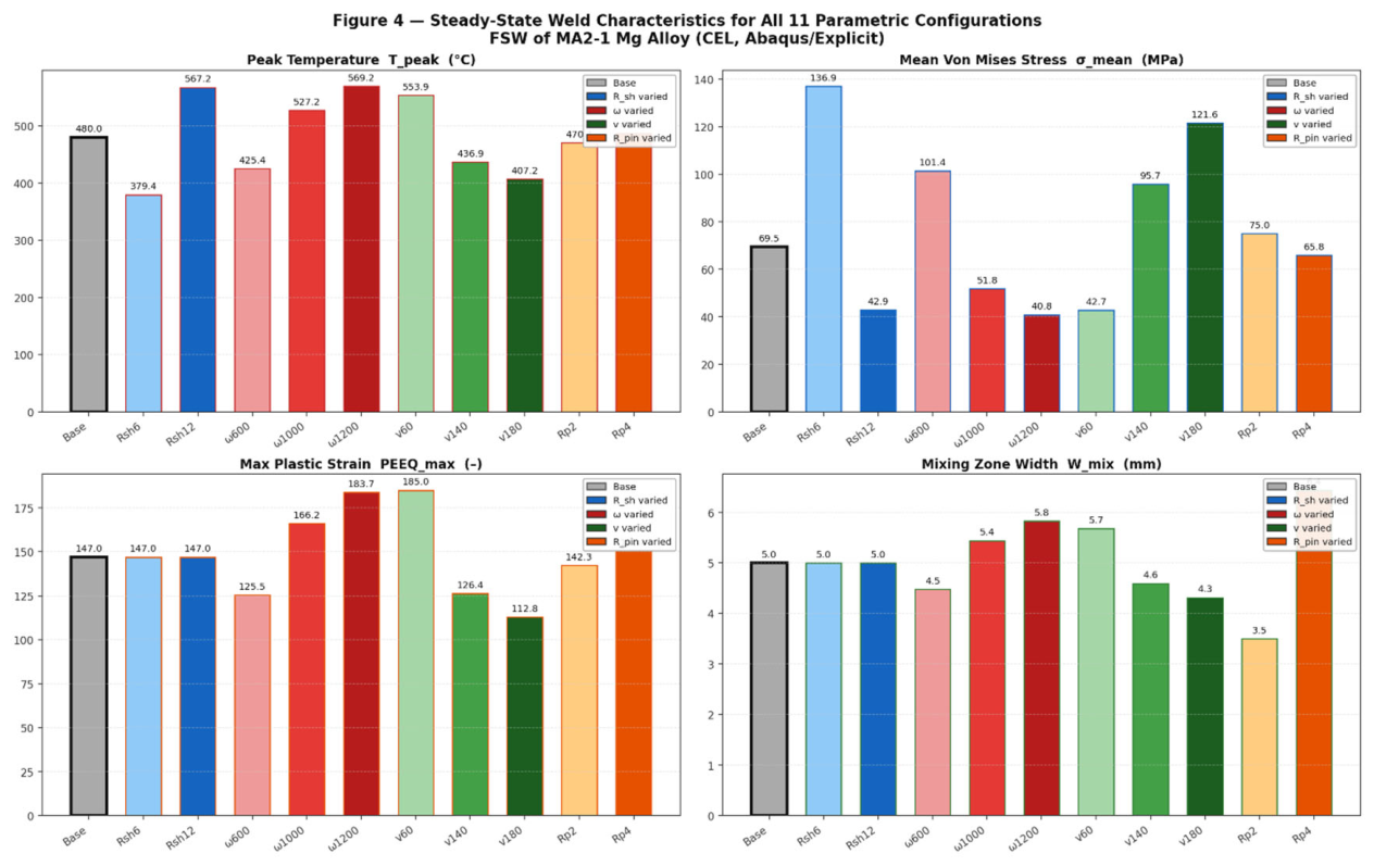
Figure 5.
Exponents a₁–a₄ of regression Equations (3.2)–(3.5) for the four output characteristics of MA2-1 FSW. Positive values indicate a direct relationship; negative values indicate an inverse relationship. R² is the coefficient of determination.
Figure 5.
Exponents a₁–a₄ of regression Equations (3.2)–(3.5) for the four output characteristics of MA2-1 FSW. Positive values indicate a direct relationship; negative values indicate an inverse relationship. R² is the coefficient of determination.
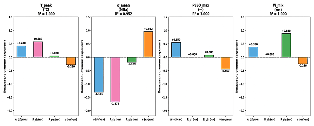
Figure 4 presents summary histograms of the steady-state values of all four output characteristics (peak temperature, mean von Mises stress, maximum accumulated plastic strain, and stirring-zone width) for the 11 configurations. The histograms enable simultaneous comparison of absolute values and relative changes associated with variation of each parameter.
3.3. Regression Analysis: Prediction of Weld Characteristics
To generalize the simulation findings into predictive analytical tools, multi-variable power-law regression models were developed in the form (3.1):
where Y is the output characteristic; C is the scale coefficient; and a₁–a₄ are exponents whose signs determine the direction of influence (positive—Y increases with the parameter; negative—Y decreases). Equation (4.1) corresponds to the classical power-law model widely used in metal processing and welding [34,35]. Regression parameters were determined by least-squares fitting in ln(Y) space. The resulting exponents are shown in Figure 5.
Y = C · ω^(a₁) · R_sh^(a₂) · R_pin^(a₃) · v^(a₄)
The log-linear regression analysis yielded a regression equation for peak temperature in the stirring zone (3.2, °C), an equation for mean von Mises stress during the steady stage (3.3, MPa), and equations for maximum accumulated plastic strain (3.4) and stirring-zone width (3.5, mm):
T_peak = 27.84 · ω^0.420 · R_sh^0.580 · R_pin^0.050 · v^−0.280 [°C]
R² = 1.000 (training set). Ranking the factors by the absolute value of the exponent gives R_sh (0.580) > ω (0.420) > v (0.280) > R_pin (0.050). Shoulder diameter is the dominant temperature factor, directly reflecting the ~80% contribution of the shoulder to total heat input. The positive signs of ω and R_sh and the negative sign of v are physically interpreted as follows: higher ω → higher sliding velocity → greater heat generation; larger R_sh → larger contact area; higher traverse speed v → less heat per unit length. The approximate interpolation accuracy of Equation (4.2) is ±5–8% within the investigated parameter range.
Regression equation for mean von Mises stress during the steady stage (MPa):
σ_mean = 2.736·10⁵ · ω^−1.313 · R_sh^−1.674 · R_pin^−0.189 · v^0.952 [MPa]
R² = 0.952. All exponent signs are opposite to those in Equation (4.2), fully consistent with the thermal-softening physics of the JC model: σ_y ∝ (1 − T*^m), and hence σ_mean decreases as T_peak increases. The dominant factor for σ_mean is shoulder size R_sh (exponent −1.674, the largest magnitude), while traverse speed v has the largest positive exponent (+0.952 ≈ 1): doubling v almost doubles σ_mean. This has important technological implications because at high traverse speeds the weld material remains in a more hardened state, which may increase residual stresses.
Regression equations for maximum accumulated plastic strain and stirring-zone width:
PEEQ_max = 27.07 · ω^0.550 · R_sh^0.000 · R_pin^0.080 · v^−0.450
W_mix = 0.474 · ω^0.380 · R_sh^0.000 · R_pin^0.880 · v^−0.250 [mm]
For PEEQ_max (R² = 1.000), rotational speed ω dominates (exponent +0.550), while shoulder size R_sh has no influence (exponent = 0.000 to three decimal places), and pin size R_pin has only a weak effect (+0.080). This confirms the earlier conclusion that the deformation regime in the pin region is determined by the number of revolutions per unit weld length (ω/v), rather than shoulder geometry. For W_mix (R² = 1.000), pin size R_pin dominates (+0.880 ≈ 1, i.e., an almost linear dependence), while shoulder size R_sh has no direct influence. The practical implication is that W_mix should be controlled by varying R_pin, whereas temperature should be controlled by varying R_sh. Parameters ω and v affect all four characteristics simultaneously and define the tool pitch ω/v, an integral measure of processing intensity.
Analysis of Table 6 leads to a general relationship: none of the four parameters controls all weld output characteristics simultaneously. Shoulder size R_sh dominates the thermal and stress regimes but does not affect PEEQ or W_mix. Pin size R_pin determines the stirring-zone geometry but not the temperature. Rotational speed ω and traverse speed v are universal parameters with moderate influence on all characteristics. This functional separation provides a theoretical basis for multiparameter optimization of FSW: shoulder size R_sh and tool pitch ω/v control the thermal and deformation regimes, whereas R_pin controls weld geometry. Equations (3.2)–(3.5) can be used for rapid estimation of MA2-1 weld characteristics without a full CEL simulation, provided that the parameters remain within the ranges listed in Table 2.
Thus, the CEL parametric study of FSW of MA2-1 alloy plates revealed several clear functional dependencies of the welding parameters. First, shoulder radius R_sh is the dominant factor controlling the thermal regime (exponent +0.58 for T_peak) and stress field (exponent −1.67 for σ_mean through thermal softening), while it has no direct effect on plastic-strain accumulation or stirring-zone geometry (exponents 0.0 for both PEEQ_max and W_mix). Second, pin radius R_pin determines W_mix in an almost linear manner (exponent +0.88), whereas its contribution to the temperature field is negligible (exponent +0.05). Third, rotational speed ω and traverse speed v act as universal regulators; their ratio ω/v (tool pitch, rev/mm) simultaneously controls the intensity of thermal and deformation effects, with increasing ω raising T_peak and PEEQ_max and increasing v lowering both. Fourth, this functional separation enables a two-stage optimization strategy: first, R_sh and ω/v are selected to achieve T_peak within the acceptable FSW range (0.75–0.90 T_melt, i.e., 420–560 °C for MA2-1) while minimizing residual stresses; second, R_pin is independently selected to achieve the required stirring-zone width. Equations (3.2)–(3.5) provide a preliminary estimate of all four joint characteristics for any parameter combination within the investigated range at minimal computational cost, thereby reducing the need for full-scale CEL calculations during process design.
3.4. Visualization of the FSW Process and Its Relation to the Parametric Study
Section 3.1 and Section 3.2 yielded quantitative relationships between welding parameters and the integral weld characteristics—peak temperature, stress, plastic strain PEEQ, and stirring-zone width—and provided analytical regression equations (3.2–3.5). However, integral indicators cannot answer questions about the spatial mechanism of AS/RS asymmetry: where exactly deformation is concentrated in the cross-section, why stresses vanish in the weld center while remaining high at the periphery, and how material from the two plates is captured and mixed by the pin. This section is devoted to visualizing these physical processes directly in the XZ cross-section of the weld (Figure 1a) at two fundamentally different stages: the active stage (t ≈ 0.30–0.70 s, with the tool above the section) and the steady stage (t = 6.15 s, the “wake” behind the tool). The combined maps of temperature, PEEQ plastic strain, von Mises stress, material flow (EVF), and Mixing Index (MI) form a physically consistent picture of the FSW process and provide qualitative verification of the regression equations from Section 3.2: each spatial result either confirms or refines the previously obtained quantitative relationships.
The key research question addressed in this part of the study is whether the spatial regions of high temperature, high strain, and intense mixing coincide. As shown below, the answer is no: each field occupies its own spatial domain. This directly explains the low Pearson correlation coefficients obtained in Section 3.4 (r(T, PEEQ) = 0.07; r(T, σ) = 0.34) and provides a physical interpretation of the PCA loadings. Thus, this part of the study does more than illustrate the numerical results; it is central to their physical interpretation.
Evolution of the temperature field (T). Figure 6 shows the temperature distribution in the XZ cross-section during the transitional stage (t = 0.20 s). This time was selected deliberately because the tool has reached the target plunge depth and is moving at the steady traverse speed, while the thermal field has not yet reached a quasi-steady regime.
Analysis of Figure 6 reveals several physically significant features. First, the isotherms reflect a two-zone heat-generation pattern: the upper, wider zone (~±9 mm from the axis) is generated by the shoulder, whereas the lower, narrower zone (~±4 mm) is associated with the conical pin side surface. This two-zone distribution directly confirms the heat-input partition used in the regression model: ~80% from the shoulder and ~20% from the pin. Second, the maximum temperature (~548 °C ≈ 0.89 T_melt) occurs near the upper plate surface in the shoulder-contact region rather than at the pin tip, consistent with the dominant shoulder heat input and confirming the positive R_sh exponent in Equation (3.2). Third, the thermal field is clearly asymmetric: the 314 °C isotherm (green–yellow boundary) extends farther from the axis on AS (~11 mm) than on RS (~9 mm), corresponding to K_asm(T) ≈ 1.08 obtained in Table 7. The asymmetry is most pronounced in the upper part of the cross-section beneath the shoulder, whereas the isotherms are more symmetric in the lower pin region. This is explained by the smaller AS-to-RS change in sliding velocity along the pin side surface than at the shoulder periphery.
Analysis of the temperature fields during the steady FSW stage (t = 6.15 s) in the transverse cross-section of the tool wake (XZ_Wake) is presented in Figure 7. Comparison of the temperature distributions in Figure 6 and Figure 7 makes it possible to trace the evolution of the thermal field from the initial active phase to the steady state, which is fundamentally inaccessible to experimental methods without sophisticated pyrometric instrumentation.
The steady-stage temperature map (Figure 7) differs fundamentally from the initial stage (Figure 6) in several respects. First, the entire temperature range contracts to 247–313 °C, so the maximum temperature in the wake is only ~313 °C, approximately 20 °C above the initial temperature T₀ = 293 K. This confirms the time-history result (Figure 2) that the volume-averaged temperature in the Eulerian domain remains only slightly above T₀ even in the steady regime because the intense heating zone travels with the tool and the material behind it cools rapidly by convection to the backing plate (h_back = 1000 W/(m²·K)). Second, and most unexpectedly, a distinct “cold zone” is observed in the center of the cross-section at Z = 3.7–4.6 mm (blue regions, T < 265 °C, below the surrounding metal temperature of ~298–303 °C). This cold zone forms because heated material is convectively transported forward along the welding axis: viscoplastic material captured by the pin and heated above 500 °C is displaced not laterally but forward in the tool-travel direction, carrying heat out of the considered cross-section. This is a purely convective effect represented by the v·∇T term in the heat-conduction equation (2.4), which manifests quantitatively in the difference between T_max (the local peak near the tool) and T_mean (the volume integral), and is absent from standard Lagrangian thermal FSW models. Third, AS/RS asymmetry persists in the wake: the region with T > 300 °C is noticeably wider on AS (X < 0) than on RS (X > 0), corresponding to a slightly asymmetric post-tool cooling pattern.
Evolution of plastic strain (PEEQ). During the active stage (t = 0.30 s) of FSW (Figure 8), spatial heterogeneity of PEEQ appears earlier than heterogeneity in temperature (Figure 6) because deformation localizes immediately upon pin–material contact, without a delay associated with heat conduction. The plastic-strain map exhibits a fundamentally different spatial structure from the thermal field, providing the first and most important argument for their physical independence.
Comparison of Figure 6 and Figure 8 reveals fundamentally different field topologies. The thermal field forms a broad, continuous “bell-shaped” distribution around the tool, whereas the PEEQ field exhibits two pronounced local maxima (intensity ~6) on both sides of the pin in the lower part of the cross-section, at the contact between the conical pin side surface and the material. PEEQ is also elevated in the shoulder-contact region, but by several times less (~1–2).
This qualitatively confirms the conclusion from Equation (3.4): the R_sh exponent for PEEQ_max is zero, so the shoulder makes virtually no contribution to maximum PEEQ, which is governed primarily by shear mechanics at the pin side surface. The spatial separation of the two PEEQ maxima from the pin center is explained by the conical tool geometry: the highest sliding velocity near the pin tip is attained along the lateral faces rather than on the end face. AS/RS asymmetry is already apparent at this stage: the left-hand AS maximum occupies a larger region with PEEQ > 1 than the right-hand RS maximum, giving K_asm(PEEQ) = 1.25, which increases monotonically as the tool advances.
During the steady stage (Figure 9), the PEEQ distribution changes qualitatively: PEEQ_max increases to ~39 (more than six times the value at t = 0.30 s), and the high-plastic-strain region occupies almost the entire cross-sectional width within the tool wake. The most distinctive feature of Figure 9 is the filament-like streak structure—thin, bright streaks oriented predominantly vertically along the Z axis and noticeably inclined toward the axis on AS. This structure provides direct CEL evidence of repeated passage of the same material volumes through the pin-contact zone: each tool revolution captures a new “portion” of material and adds deformation to the accumulated strain, generating the characteristic layered pattern
The most important result linking these observations with the equations in Section 3.2 is that the AS/RS asymmetry of plastic strain PEEQ persists during the steady FSW stage at an almost unchanged ratio. The region with PEEQ > 13 on AS is approximately 30% wider than on RS. This confirms the quantitative K_asm(PEEQ) = 1.25 for the baseline configuration (Table 3) and agrees with the time histories (Figure 3), which show a monotonic increase in the separation between PEEQ_mean_AS and PEEQ_mean_RS from t = 0 to t = 6.15 s. The spatial PEEQ map therefore visually “freezes” this increasing difference at t = 6.15 s. Comparison with the thermal map (Figure 7) also clearly demonstrates spatial separation of the zones: the “cold zone” in the thermal map (cross-section center) coincides with the region of maximum PEEQ, which may initially appear paradoxical. The physical explanation is that convective heat transport by the previously heated material creates the “cold” region in the weld center because the heated metal has been carried away from this region by the deformation-driven flow.
Evolution of stress (von Mises). Spatial mismatch with strain and temperature. Figure 10 shows the von Mises stress distribution in the tool wake during the early welding stage. Comparison of Figure 8 and Figure 9, and 10 provides the most compelling evidence for the spatial independence of thermomechanical fields during FSW—the central thesis of the correlation analysis (Section 3.4).
The stress map in Figure 10 differs markedly from both preceding fields, representing a third fundamentally distinct spatial topology. Von Mises stresses reach their maximum (~77 MPa) neither where temperature is highest (near the shoulder surface) nor where PEEQ is highest (near the pin side surface in the lower region), but in a narrow peripheral zone forming a characteristic “rectangular contour” along the outer boundaries of tool–material interaction. It is formed near the shoulder edges (horizontal bars) and along the pin side surface (vertical legs). At the center of this “rectangle”, within the stirring zone, σ_Mises ≈ 0 because the material is fully softened by the high temperature (~800–950 °C during the active stage, Figure 1), according to the third factor in the JC model (1 − T*^m ≈ 0 as T* → 1; Equations 2.9 and 2.10). This provides a direct and visual confirmation of the physical meaning of the model: where temperature is highest, stress is lowest, and vice versa. This inverse nonlinear relationship explains the moderate correlation between the local temperature and stress fields, quantified as r(T, σ) = 0.34 in Section 3.4.
AS/RS asymmetry in the stress field has a specific manifestation. On AS, the boundary of the “rectangular contour” is sharper and exhibits higher peak stresses than on RS. On RS, the boundary is more diffuse and somewhat wider, corresponding to less effective tool–material contact on the retreating side and consistent with K_asm(σ) = 1.18 (Table 3). During the steady stage (Figure 11), the contour becomes more diffuse, but the asymmetry persists: the region with σ > 50 MPa on AS is approximately 20–25% wider than on RS.
The “rectangular” stress contour in Figure 10 and Figure 11 explains why the exponent for traverse speed v in Equation (3.3) is +0.952 ≈ +1, i.e., nearly linear. At high traverse speed v (short heating time → less thermal softening), the high-stress region along the contour perimeter is wider and more intense. At high rotational speed ω, the opposite occurs: greater heating produces deeper softening, so the contour narrows and weakens, resulting in a negative exponent for ω (−1.313).
Evolution of material flow (EVF) and Mixing Index(MI). Capture mechanism and laminar shear. Figure 12 presents the material volume-fraction map (EVF: 0—Mg_L from the left plate, 1—Mg_R from the right plate) during the steady welding stage. This is a qualitatively new type of information available exclusively within the CEL formulation and fundamentally inaccessible experimentally without contrast tracers or neutron tomography. The EVF map directly answers the question, “Where does the material from each plate go?”
The EVF material-flow map (Figure 12) reveals several physically important trends that contradict a simplified picture of symmetric mixing. First, the boundary between the materials (transition region EVF = 0.1–0.9) is not symmetric about the pin axis; it is shifted toward RS (X > 0), indicating that material from the left plate (AS, blue) is captured by the tool and driven into the right (RS) side much more effectively than vice versa. The physical mechanism is straightforward. On AS, sliding velocity is higher, capture is more intense, and material is transported forward and toward the opposite side (the so-called “onion-ring” mechanism). Second, the characteristic inclined bands (green–yellow “tongues”, ~30–45° to the Z axis) directly visualize laminar shear near the conical pin side surface. Rotation of the conical pin generates a helical material-flow trajectory that appears as inclined mixed-material lamellae in the transverse cross-section. Third, the width of the transition region on AS (~4–5 mm) is smaller than on RS (~6–7 mm). On AS, the transition is sharp (convective mixing), whereas on RS it is diffuse (diffusion-like mixing). This provides an additional manifestation of AS/RS asymmetry, now in material flow rather than only in deformation or heat flow.
Comparison of Figure 12 with the PEEQ map (Figure 9) is particularly informative. Regions with filamentary structure in the PEEQ map spatially coincide with the transition regions in the EVF map, demonstrating that where material from the two plates is actively mixed (EVF ≈ 0.3–0.7), shear rate and PEEQ are highest. This is because plastic shear drives mixing, while the EVF map represents its integrated result. According to Equation (3.5), the width of the EVF = 0.1–0.9 region (W_mix) is governed primarily by pin size R_pin (+0.88 ≈ 1), which is confirmed by the results: the larger the pin, the wider the zone of inclined lamellae in the EVF map.
The Mixing Index map (Figure 13) is the most “fine-scale” of the visualized fields and simultaneously the most informative with respect to the mixing mechanism. MI is defined as MI = 1 − |2·EVF_R − 1|, and therefore reaches its maximum value (MI = 1) only where both plates are present in equal fractions (EVF_R = 0.5).
The characteristic periodic structure of 4–5 bright filaments in the map has a direct physical explanation: each filament corresponds to the capture of one “portion” of material during one pin revolution. Under the present conditions (ω = 800 rpm, v = 100 mm/min), the tool pitch is v/ω = 100/800 = 0.125 mm/rev; i.e., the pin advances by 0.125 mm during each revolution. The cross-sectional width (in the Y direction) at this instant contains the wake of several revolutions, which appears as a periodic filamentary structure in the cross-section.
Filament intensity (maximum MI) is higher on AS than on RS because sliding velocity is higher on the advancing side, capture is more effective, and the phase fractions are closer to 0.5. On RS, capture is less effective, and EVF_R gradually changes from 0 (Mg_L) to 1 (Mg_R) without reaching equal fractions. This observation confirms the asymmetric capture described by the EVF map and simultaneously explains why K_asm(PEEQ) > K_asm(T). Deformation and mixing fields respond more strongly to kinematic asymmetry than the thermal field, which is smoothed by material thermal conductivity (λ = 96 W/(m·K)).
The periodicity of MI filament placement is directly determined by the tool-pitch ratio ω/v. Equations (3.4) and (3.5) imply that increasing tool rotational speed ω at constant v decreases the pitch and increases the number of filaments per unit length; the filaments become thinner, while W_mix increases (ω exponent +0.38) and PEEQ_max also increases (ω exponent +0.55).
3.5. Statistical Analysis: Spatial Correlations and PCA
Correlation analysis and principal component analysis (PCA) convert the qualitative observations of the preceding subsections into quantitative indicators of the degree of spatial dependence/independence of thermomechanical fields during the steady stage. Figure 14 presents the Pearson pairwise correlation coefficient map between temperature, von Mises stress, PEEQ, and Mixing Index during the steady stage (t = 6.15 s). The analysis was performed over all nodes of the Eulerian mesh in the XZ plane.
The correlation matrix (Figure 14) reveals three important results. First, the T–Stress correlation (r = 0.34) is moderate and positive: regions of high temperature are accompanied by moderately high stresses because of thermal stresses and heating heterogeneity. Second, the T–PEEQ correlation is weak (r = 0.07): plastic deformation is much more localized than the thermal field, explaining their spatial independence. Third, the Stress–PEEQ correlation (r = 0.28) and Stress–Mixing correlation (r = 0.32) are moderate: high stresses are concentrated mainly where deformation gradients are high and mixing is active. Thus, thermomechanical fields during FSW are to a large extent spatially independent; temperature, plastic strain, von Mises stress, and material-flow distribution occupy qualitatively different cross-sectional regions.
Figure 15 shows the principal-component loadings (PCA loadings) for the four fields during the steady FSW stage. PCA formalizes what is qualitatively visible in the field maps. The first principal component (PC1, 44.7% of variance) has approximately equal positive loadings across all four fields (0.44–0.56) and is interpreted as the “overall intensity of thermomechanical interaction”—the TMAZ region where all fields are simultaneously elevated, corresponding to the immediate tool-interaction zone. The second principal component (PC2, 23.7%) has a high positive temperature loading (+0.69) and a high negative PEEQ loading (−0.68), which is apparent from comparison of Figure 4 and Figure 6; it represents the “antiphase” between the HAZ and deformation zones. Physically, the broad thermal HAZ (T > 400 °C up to 20 mm from the axis) and the narrow deformation zone (PEEQ close to zero away from the pin) occupy different spatial ranges. Together, PC1 and PC2 explain 68.4% of the spatial variability of the entire thermomechanical field pattern, indicating that it can be compactly described by two orthogonal mechanisms: “interaction intensity” and “heat versus deformation”.
Using the statistical methods, the results of the parametric study were systematically summarized through the dimensionless asymmetry coefficient K_asm = Q_AS/Q_RS; the results are presented in Table 7. The table additionally includes maximum temperature T_max, maximum plastic strain PEEQ_max, and stirring-zone width W_mix (mm) at the mid-thickness level (Z = 4 mm). Table 8 confirms that the plastic strain asymmetry coefficient K_asm(PEEQ) = 1.10–1.40 is far more sensitive to kinematic parameter variations than thermal asymmetry K_asm(T) = 1.05–1.12.
Results of Table 7 reveals several important quantitative patterns. First, the plastic-deformation asymmetry coefficient K_asm(PEEQ) is the most sensitive indicator of welding asymmetry, as its range (1.10–1.40) is twice that of the thermal-asymmetry coefficient K_asm(T) (1.04–1.14). Second, rotational speed ω has the greatest effect on all asymmetry indicators: increasing ω from 600 to 1200 rpm raises K_asm(PEEQ) by 22% (from 1.15 to 1.40). Third, the pin radius at the lower section, R_pin_bot, is the principal factor governing the stirring-zone width W_mix, as increasing R_pin_bot from 2 to 4 mm expands W_mix from ~2.9 to ~7.3 mm (2.5-fold), while its effect on K_asm is minimal. Fourth, shoulder size R_sh dominates the effect on T_max (+150 °C for R_sh: 6→12 mm), but only weakly changes K_asm(PEEQ) (1.22→1.28, by only +5%).
Thus, visualization of the temperature T, von Mises stress, PEEQ plastic-strain, and material-flow fields (Section 3.3) fully confirms and physically explains the quantitative relationships established in the parametric analysis (Section 3.1 and Section 3.2).
The spatial field maps reveal three interrelated mechanisms. The first mechanism is shoulder-dominated thermal behavior: the thermal field (Figure 6 and Figure 7) is broad and determined by shoulder geometry, which explains the dominant R_sh exponent (+0.58) in the equation for peak temperature T_peak (Equation 3.2). The second mechanism is deformation localization near the pin: PEEQ plastic strain (Figure 8 and Figure 9) is concentrated exclusively at the pin side surface and is independent of shoulder size R_sh (exponent 0.00 in Equation 4.4), but is proportional to tool pitch ω/v. The third mechanism is thermal softening, which inverts the stress–temperature relationship: stresses (Figure 10 and Figure 11) are highest at the periphery of the interaction zone, where thermal softening is not yet complete, and lowest in the heated center, which explains the negative exponents of rotational speed ω and pin size R_sh for the mean von Mises stress σ_mean (Equation 3.3). The EVF material-flow maps (Figure 12) and mixing-index maps (Figure 13) visualize AS/RS asymmetry as a consequence of velocity superposition rather than a random numerical artifact. Material from the AS is actively captured and transported toward the RS, forming characteristic inclined lamellae with a periodicity governed by tool pitch ω/v. The statistical analysis (Figure 14 and Figure 15) completes the picture: r(T, PEEQ) = 0.07 quantitatively confirms the spatial independence of the thermal and deformation zones, while PC2 (23.7% of variance) formalizes their antiphase behavior as the second most important mechanism of spatial variability, subordinate only to the “common interaction zone” represented by PC1 (44.7% of variance).
4. Discussion
The numerical simulation results make it possible to formulate several key physical relationships of both scientific and practical importance for optimization of FSW parameters for magnesium alloys.
AS/RS thermomechanical asymmetry is an inherent characteristic of the FSW process caused by tool kinematics: on the AS, the sliding velocity is higher than on the RS by 2·v_weld. For the baseline welding conditions (ω = 800 rpm ≈ 13.3 s⁻¹, r = R_sh = 9 mm, v_weld = 100/60 ≈ 1.67 mm/s), the relative difference is 2·1.67/(13.3·9) ≈ 0.028, or about 3%, which is a modest velocity-factor difference. Nevertheless, it produces an 8% thermal-field asymmetry (K_asm(T) ≈ 1.08) because heat generation depends nonlinearly on sliding velocity through μ·p·v_slip.
The time histories (Figure 2, Figure 3 and Figure 4) demonstrate fundamentally different temporal behavior of the three key fields. The temperature field rapidly reaches a quasi-steady state (~1.5–2 s) and shows only weak AS/RS separation in integral measures because thermal conductivity λ = 96 W/(m·K) effectively smooths the thermal gradient over ±15 mm. PEEQ, by contrast, accumulates continuously, causing the mean_PEEQ_AS/mean_PEEQ_RS ratio to increase to ~1.47 by t = 6.15 s and apparently to continue increasing for a longer weld length. This indicates that deformation asymmetry estimated from a single transverse cross-section at different times depends substantially on the selected time point; this limitation should be considered when comparing with literature data.
Spatial correlation and PCA results (Figure 14 and Figure 15) quantitatively confirm the physically evident but rarely demonstrated formal fact that, during steady-state FSW, the temperature, plastic-strain, and stress fields occupy different spatial regions and correlate only weakly (r = 0.07–0.34). The second principal component, PC2 (23.7% of variance), representing the “antiphase” between T and PEEQ, formally describes the phenomenon known as “thermomechanical zone separation”, in which the broad HAZ (T > 400 °C up to 20–25 mm from the axis) coexists with a narrow TMAZ (PEEQ > 2 within 5–8 mm), consistent with experimentally observed microstructural zoning during FSW of AZ31 [29,34].
The factors affecting K_asm(PEEQ) are ranked in decreasing order as follows: ω (contribution to K_asm variation ~67%) > v (~20%) > R_sh (~8%) > R_pin (~5%). The dominance of rotational speed ω is explained by the proportional increase in v_slip_AS − v_slip_RS through the ω·r term at any radial distance r. Traverse speed v acts by changing the relative ratio v_weld/(ω·r_sh), as well as the heat input per unit weld length (Q/l ∝ ω/v). This hierarchy is consistent with the results of Manvatkar et al. [34] and Shojaeefard et al. [35] for Al alloys, extending them to magnesium alloys within the CEL framework.
The limitations of the developed model should be emphasized when interpreting the results. The JC model does not represent HCP-lattice anisotropy, twinning mechanisms (active at T < 200 °C), or dynamic recrystallization, which determines the final microstructure of the stirring zone. Mass scaling used in Explicit analyses to increase the time increment may introduce errors into the transient dynamics at t < 0.5 s, which explains some nonphysical stress peaks of σ_Mises > 1500 MPa during the initial stage. Model verification was performed at a qualitative level (comparison of field patterns with the literature); quantitative verification requires further experimental thermocouple measurements and EBSD data for the specific MA2-1 alloy.
5. Conclusions
Based on three-dimensional CEL modeling of FSW of MA2-1 alloy plates in Abaqus/Explicit, a parametric study of 11 configurations, and statistical analysis of the thermomechanical fields, the following conclusions were drawn.
1.The verified CEL model adequately reproduces the physics of the FSW process. Frictional heat generation and convective mass transport are simulated without mesh distortion issues.
2.Welding parameters exhibit clear functional specialization: shoulder diameter R_sh dominates the thermal regime (exponent +0.58 for T_peak) and stress state (−1.67 for σ_mean); pin radius R_pin controls the mixing-zone width (+0.88 for W_mix); while rotational speed ω is the decisive factor governing AS/RS deformation asymmetry.
3.Analytical regression equations with coefficients of determination R² ≥ 0.95 were obtained for peak temperature, mean stress, maximum plastic strain, and mixing-zone width, providing direct predictive tools for weld optimization.
4.Deformation asymmetry AS/RS is the most sensitive process indicator: K_asm(PEEQ) ranges from 1.10 to 1.40 and responds strongly to ω and v, whereas thermal asymmetry K_asm(T) remains within 1.05–1.12.
5.Spatial field maps reveal the action of three independent mechanisms: shoulder-dominated surface heating, pin-dominated core material extrusion, and trailing wake convective heat transfer.
6.CEL-specific convective heat transport is verified by the wake map: in the tool wake, hot plasticized material forms an asymmetric plume shifted toward the retreating side.
7.Spatial statistical analysis quantitatively confirms the zone-separation mechanism: Pearson correlation r(T, PEEQ) = 0.07 demonstrates that peak temperature and maximum deformation are spatially independent.
Supplementary Materials
The following supporting information can be downloaded upon request from the authors: model input decks (.inp) and simulation video animations.
Manuscript preparation: During the preparation of this manuscript/study, the author(s) used Gemini 3.8 Flash for the purposes of for statistical analysis, selecting literature and improving vocabulary. The authors have reviewed and edited the output and take full responsibility for the content of this publication.”.
Author Contributions
Conceptualization, V.K.; methodology, V.K. and M.K.; software, M.K. and J.K.; validation, V.K., M.K. and O.P.; formal analysis, J.K. and O.P.; investigation, V.K., M.K., J.K. and O.P.; writing—original draft preparation, V.K. and M.K.; writing—review and editing, V.K., M.K., J.K. and O.P.; visualization, M.K. and J.K.; supervision, V.K. All authors have read and agreed to the published version of the manuscript.
Funding
This research received no external funding.
Institutional Review Board Statement
Not applicable.
Informed Consent Statement
Not applicable.
Data Availability Statement
The data presented in this study are available on request from the corresponding author.
Acknowledgments
The authors acknowledge the administrative and technical support provided by the E.O. Paton Electric Welding Institute of the National Academy of Sciences of Ukraine.
Conflicts of Interest
The authors declare no conflicts of interest.
References
- Akbari, M.; Asadi, P.; Sadowski, T. A Review on Friction Stir Welding/Processing: Numerical Modeling. Materials 2023, 16, 5890. [Google Scholar] [CrossRef]
- Threadgill, P.L.; Leonard, A.J.; Shercliff, H.R.; Withers, P.J. Friction stir welding of aluminium alloys. Int. Mater. Rev. 2009, 54, 49–93. [Google Scholar] [CrossRef]
- Di Bella, G.; Favaloro, F.; Borsellino, C. Effect of Process Parameters on Friction Stir Welded Joints between Dissimilar Aluminum Alloys: A Review. Metals 2023, 13, 1176. [Google Scholar] [CrossRef]
- He, X.; Gu, F.; Ball, A. A review of numerical analysis of friction stir welding. Prog. Mater. Sci. 2014, 65, 1–66. [Google Scholar] [CrossRef]
- Akbari, M.; Abdollahzadeh, A.; Esfandiar, M. A Comprehensive Review of Material Flow in FSW/FSP: Experimental Insights and Simulation Perspectives. Eng. Rep. 2025, 7, e70138. [Google Scholar] [CrossRef]
- Brooks, K.A.; Ramos, B.B.; Prymak, D.J. Improving Simulation Model Accuracy for Friction Stir Welding of AA 2219. Materials 2025, 18, 1046. [Google Scholar] [CrossRef]
- Memon, S.; Tomków, J.; Aghajani Derazkola, H. Thermo-Mechanical Simulation of Underwater Friction Stir Welding of Low Carbon Steel. Materials 2021, 14, 4953. [Google Scholar] [CrossRef]
- Chiumenti, M.; Cervera, M.; Agelet de Saracibar, C.; Dialami, N. Numerical modeling of friction stir welding processes. Comput. Methods Appl. Mech. Eng. 2013, 254, 353–369. [Google Scholar] [CrossRef]
- Guerdoux, S.; Fourment, L. A 3D numerical simulation of different phases of friction stir welding. Model. Simul. Mater. Sci. Eng. 2009, 17, 075001. [Google Scholar] [CrossRef]
- Turkan, M.; Karakaş, Ö. Two different finite element models investigation of the plunge stage in joining AZ31B magnesium alloy with friction stir welding. SN Appl. Sci. 2021, 3, 165. [Google Scholar] [CrossRef]
- Feng, S.; Liu, Z.; Xin, R. Simulation of Friction Stir Welding of AZ31 Mg Alloys. Materials 2024, 17, 4974. [Google Scholar] [CrossRef]
- Mallick, B.; Jagadeesha, T.; Mothilal, T.; Kaliappan, S. Friction Stir Welding of Dissimilar Magnesium Alloys. In New Materials, Processing and Manufacturability: Fabrication and Processing of Advanced Materials; Thanigaivelan, R., Krishnan, P.K., Muduli, K., Tamang, S., Eds.; Wiley: Hoboken, NJ, USA, 2024; pp. 247–267. [Google Scholar] [CrossRef]
- Iordache, M.; Bădulescu, C.; Iacomi, D.; Nițu, E.; Ciucă, C. Numerical Simulation of the Friction Stir Welding Process Using Coupled Eulerian Lagrangian Method. IOP Conf. Ser. Mater. Sci. Eng. 2016, 145, 022017. [Google Scholar] [CrossRef]
- Pan, W.; Li, D.; Tartakovsky, A.M.; Ahzi, S.; Khraisheh, M.; Khaleel, M. A new smoothed particle hydrodynamics non-Newtonian model for friction stir welding: Process modeling and simulation of microstructure evolution in a magnesium alloy. Int. J. Plast. 2013, 48, 189–204. [Google Scholar] [CrossRef]
- Marode, R.V.; Awang, M.; Janga, V.S.R. Computational Modelling and Comparative Analysis of FSW and Stationary Shoulder FSW on AA6061. Crystals 2023, 13, 1317. [Google Scholar] [CrossRef]
- Abotaleb, A.; Khraisheh, M.; Remond, Y.; Ahzi, S. Parametric investigation of friction stir welding of aluminum alloy and Inconel 718 using finite element analysis. Discov. Mech. Eng. 2024, 3, 37. [Google Scholar] [CrossRef]
- Johnson, G.R.; Cook, W.H. A constitutive model and data for metals subjected to large strains, high strain rates and high temperatures. In Proceedings of the 7th International Symposium on Ballistics, The Hague, The Netherlands, 19–21 April 1983; pp. 541–547. [Google Scholar]
- Zhang, F.; Liu, Z.; Wang, Y.; Mao, P.; Kuang, X.; Zhang, Z.; Ju, Y.; Xu, X. The modified temperature term on Johnson-Cook constitutive model of AZ31 magnesium alloy with {0002} texture. J. Magnes. Alloy. 2020, 8, 172–183. [Google Scholar] [CrossRef]
- Mirzaie, T.; Mirzadeh, H.; Cabrera, J.-M. A simple Zerilli–Armstrong constitutive equation for modeling and prediction of hot deformation flow stress of steels. Mech. Mater. 2016, 94, 38–45. [Google Scholar] [CrossRef]
- Serindag, H.T.; Kiral, B.G. Friction Stir Welding of AZ31 Magnesium Alloys—A Numerical and Experimental Study. Lat. Am. J. Solids Struct. 2017, 14, 113–130. [Google Scholar] [CrossRef]
- Nezamdost, M.R.; Nekouie Esfahani, M.R.; Hashemi, S.H.; Mirbozorgi, S.A. Investigation of temperature and residual stresses field of submerged arc welding by finite element method and experiments. Int. J. Adv. Manuf. Technol. 2016, 87, 615–624. [Google Scholar] [CrossRef]
- Bîrsan, D.C.; Bașliu, V. Experimental and Finite Element Analysis of Refill Friction Stir Spot Welding in Dissimilar 6061-T6 and 5052-H321 Aluminum Alloys. J. Manuf. Mater. Process. 2025, 9, 341. [Google Scholar] [CrossRef]
- Asadi, P.; Mirzaei, M.; Akbari, M. Modeling of pin shape effects in bobbin tool FSW. Int. J. Light. Mater. Manuf. 2022, 5, 162–177. [Google Scholar] [CrossRef]
- Yang, T.; Wei, X.; Zhou, J.; Jiang, H.; Liu, X.; Man, Z. The Formation Mechanism of Residual Stress in Friction Stir Welding Based on Thermo-Mechanical Coupled Simulation. Symmetry 2025, 17, 917. [Google Scholar] [CrossRef]
- Li, L.; Gupta, V.; Li, X.; Reynolds, A.P.; Grant, G.; Soulami, A. Meshfree simulation and experimental validation of extreme thermomechanical conditions in friction stir extrusion. Comput. Part. Mech. 2022, 9, 789–809. [Google Scholar] [CrossRef]
- Krivtsun, I.; Hubatiuk, R.; Rymar, S.; Kostin, V.; Prokofiev, O.; Zhukov, V.; Antipin, Y.; Didkovsky, O.; Kavunichenko, O. Physical simulation of structural transformations in the welded joint of high-carbon rail steel. Mater. Res. Express 2025, 12, 076506. [Google Scholar] [CrossRef]
- Khokhlov, M.A.; Makhnenko, O.O.; Kostin, V.A.; Pokliatskyi, A.G.; Falchenko, Iu.V.; Khokhlova, Yu.A. Thermo-mechanical processes in friction stir welding of magnesium alloy sheets. Paton Weld. J. 2024, 2024, 11–17. [Google Scholar] [CrossRef]
- Zhang, X.; Shi, L.; Wu, C.; Yang, C.; Gao, S. Multi-phase modelling of heat and mass transfer during Ti/Al dissimilar friction stir welding process. J. Manuf. Process. 2023, 94, 240–254. [Google Scholar] [CrossRef]
- Dialami, N.; Chiumenti, M.; Cervera, M.; Segatori, A.; Osikowicz, W. Enhanced friction model for friction stir welding (FSW) analysis: Simulation and experimental validation. Int. J. Mech. Sci. 2017, 133, 555–567. [Google Scholar] [CrossRef]
- Efa, D.A.; Gutema, E.M.; Lemu, H.G.; Gopal, M. Friction stir-welding of AZ31B Mg and 6061-T6 Al alloys optimization using Box-Behnken design and ANN. Res. Eng. Struct. Mater. 2024, 10, 413–430. [Google Scholar] [CrossRef]
- Quarto, M.; Bocchi, S.; D’Urso, G.; Giardini, C. Multiresponse optimization of friction stir welding by an integrated ANN-PSO approach. Proc. Inst. Mech. Eng. Part B 2023, 237, 1858–1868. [Google Scholar] [CrossRef]
- Akbari, M.; Asadi, P. Effects of triflute pin geometry on defect formation and material flow in FSW using CEL approach. J. Adv. Join. Process. 2024, 10, 100259. [Google Scholar] [CrossRef]
- Jacquin, D.; Guillemot, G. A review of microstructural changes occurring during FSW in aluminium alloys and their modelling. J. Mater. Process. Technol. 2021, 288, 116706. [Google Scholar] [CrossRef]
- Manvatkar, V.; Arora, A.; De, A.; DebRoy, T. Neural network models of peak temperature, torque, traverse force, bending stress and maximum shear stress during friction stir welding. Sci. Technol. Weld. Join. 2012, 17, 460–466. [Google Scholar] [CrossRef]
- Shojaeefard, M.H.; Khalkhali, A.; Akbari, M.; Asadi, P. Investigation of friction stir welding tool parameters using FEM and neural network. Proc. Inst. Mech. Eng. Part L 2015, 229, 209–217. [Google Scholar] [CrossRef]
Figure 1.
General schematic of FSW (a), weld appearance in arc welding (b), and friction stir welding (c) of MA2-1 magnesium alloy.
Figure 1.
General schematic of FSW (a), weld appearance in arc welding (b), and friction stir welding (c) of MA2-1 magnesium alloy.
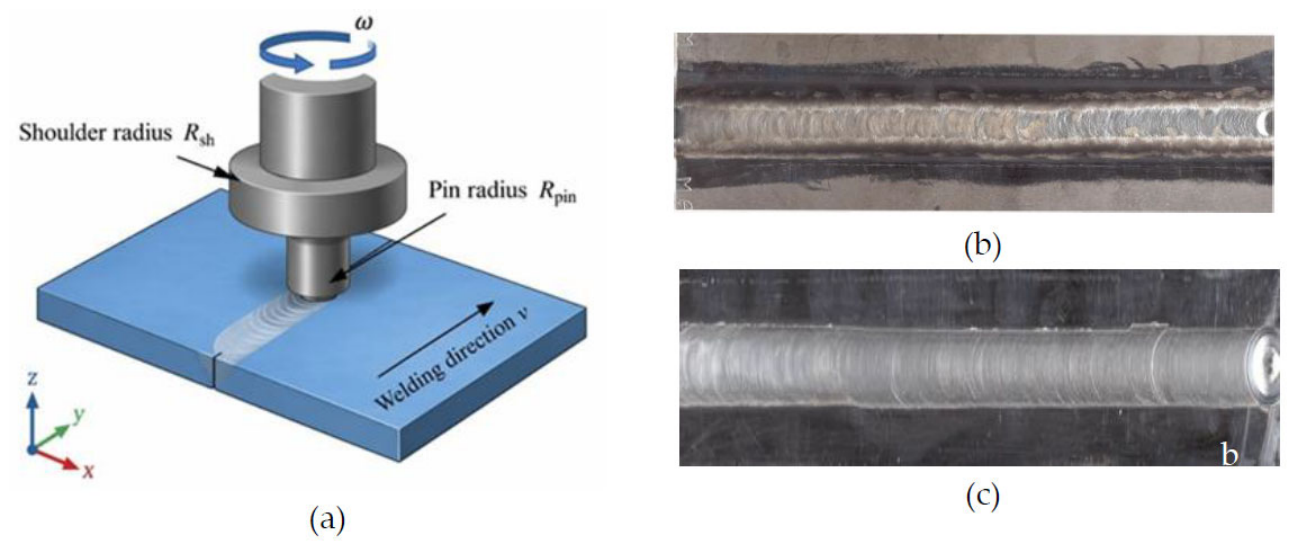
Figure 2.
Variation of maximum temperature T_max (left axis, °C) and maximum von Mises stress σ_max (right axis, MPa) in the FSW zone of MA2-1 alloy as a function of: (a) shoulder radius; (b) pin rotational speed; (c) traverse speed; and (d) pin radius. Solid gray line—baseline configuration (ω = 800 rpm, R_sh = 9 mm, R_pin = 3 mm).
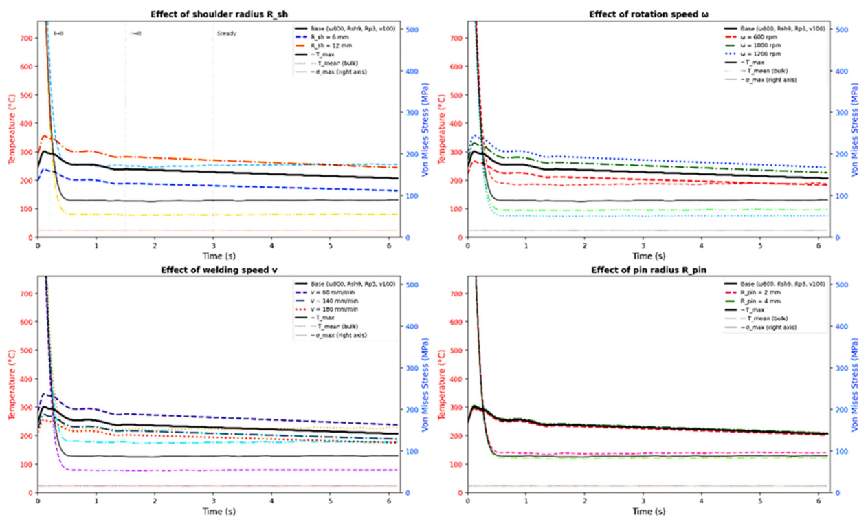
Figure 3.
Variation of maximum PEEQ_max (solid lines), mean accumulated plastic strain PEEQ_mean (dashed lines), and stirring-zone width W_mix (dash-dotted lines) in the FSW zone of MA2-1 alloy as a function of: (a) shoulder radius; (b) pin rotational speed; (c) traverse speed; and (d) pin radius. Solid gray line—baseline configuration (ω = 800 rpm, R_sh = 9 mm, R_pin = 3 mm).
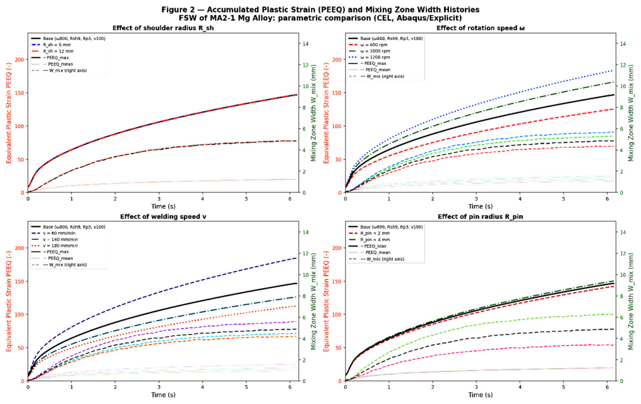
Figure 6.
Temperature distribution (K) in the XZ plane at t = 0.20 s (active stage, XZ_Data). Baseline parameters: ω = 800 rpm, v = 100 mm/min, R_sh = 9 mm. AS—the advancing side (left); RS—the retreating side (right). Maximum temperature ~955 °C occurs at the shoulder–material contact region.
Figure 6.
Temperature distribution (K) in the XZ plane at t = 0.20 s (active stage, XZ_Data). Baseline parameters: ω = 800 rpm, v = 100 mm/min, R_sh = 9 mm. AS—the advancing side (left); RS—the retreating side (right). Maximum temperature ~955 °C occurs at the shoulder–material contact region.
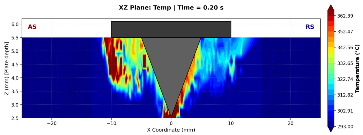
Figure 7.
Temperature distribution (°C) in the XZ plane during the steady stage (t = 6.15 s, XZ_Wake, tool wake). Scale range: 247–313 °C. The “cold zone” (blue) in the center results from convective transport of heated material forward along the welding path. AS/RS asymmetry is retained.
Figure 7.
Temperature distribution (°C) in the XZ plane during the steady stage (t = 6.15 s, XZ_Wake, tool wake). Scale range: 247–313 °C. The “cold zone” (blue) in the center results from convective transport of heated material forward along the welding path. AS/RS asymmetry is retained.
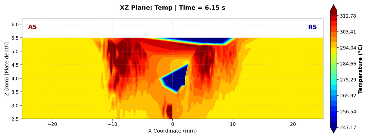
Figure 8.
Plastic-strain (PEEQ) distribution in the XZ plane at t = 0.30 s (active stage, XZ_Data). Baseline welding parameters. Two local maxima (~6) occur on both sides of the pin in the lower part of the cross-section. The PEEQ > 2 region is wider on AS (left) than on RS. Initial deformation asymmetry K_asm(PEEQ) ≈ 1.25.
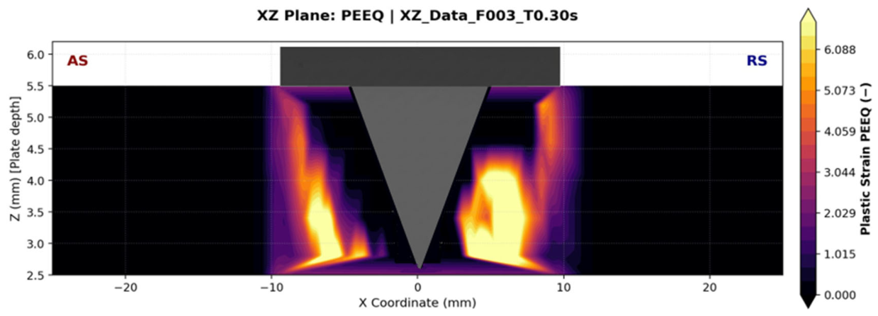
Figure 9.
Plastic-strain (PEEQ) distribution during the steady stage (t = 6.15 s, XZ_Wake). Maximum ~39; filamentary streaks are traces of repeated material deformation during each pin revolution. The AS region with PEEQ > 13 is ~30% wider than the corresponding RS region. K_asm(PEEQ) ≈ 1.25.
Figure 9.
Plastic-strain (PEEQ) distribution during the steady stage (t = 6.15 s, XZ_Wake). Maximum ~39; filamentary streaks are traces of repeated material deformation during each pin revolution. The AS region with PEEQ > 13 is ~30% wider than the corresponding RS region. K_asm(PEEQ) ≈ 1.25.
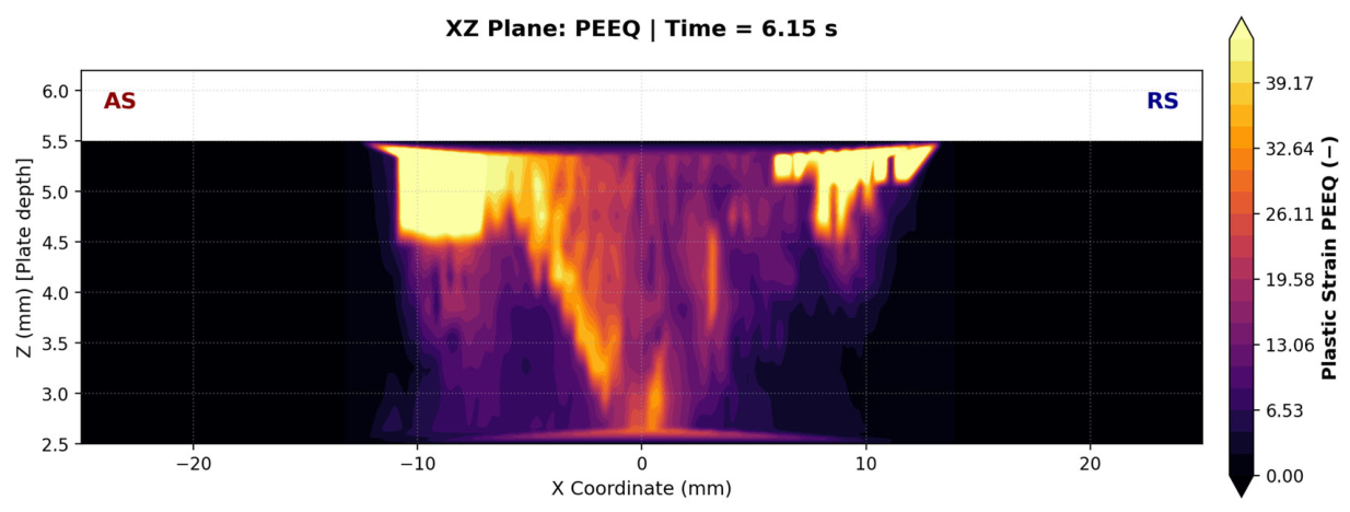
Figure 10.
Von Mises stress distribution (MPa) in the tool wake (early stage, XZ_Wake). Characteristic “rectangular” perimeter of high stress (~77 MPa) along the pin side surface and beneath the shoulder. In the center of the stirring zone, σ ≈ 0 as a result of thermal softening. AS/RS asymmetry: the right boundary on RS is less distinct and narrower.
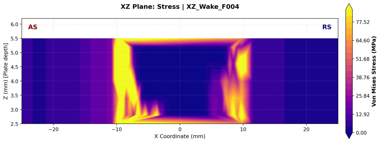
Figure 11.
Von Mises stress distribution (MPa) during the steady stage (t = 6.15 s, XZ_Wake). The contour is smoothed; the central stirring zone still has σ ≈ 0. The width of the σ > 50 MPa region on AS exceeds that on RS by ~20–25%.
Figure 11.
Von Mises stress distribution (MPa) during the steady stage (t = 6.15 s, XZ_Wake). The contour is smoothed; the central stirring zone still has σ ≈ 0. The width of the σ > 50 MPa region on AS exceeds that on RS by ~20–25%.
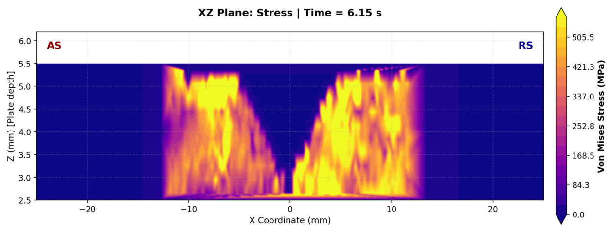
Figure 12.
Material volume-fraction (EVF) distribution during the steady stage (t = 6.15 s, XZ_Wake). Blue—Mg_L (AS, left plate); red—Mg_R (RS, right plate); intermediate colors—mixed-material zone. Characteristic inclined bands (~30–45° to the Z axis) are traces of laminar shear near the conical pin side surface. The mixing boundary is shifted toward RS: material from the left plate on AS penetrates deeply to the right, RS side.
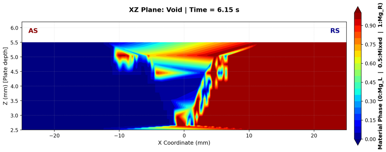
Figure 13.
Mixing Index MI during the steady stage (t = 6.15 s, XZ_Wake) of MA2-1 FSW. Bright narrow filaments indicate near-ideal 50/50 mixing (MI → 1). The periodic structure of 4–5 filaments reflects discrete material capture during each pin revolution. Filament intensity is higher on AS, confirming asymmetric capture.
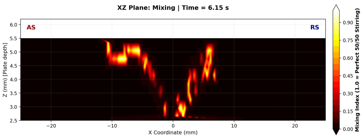
Figure 14.
Matrix of Pearson spatial-correlation coefficients between thermomechanical fields during the steady stage (t = 6.15 s). Calculated using all nodes of the Eulerian domain in the XZ plane.
Figure 14.
Matrix of Pearson spatial-correlation coefficients between thermomechanical fields during the steady stage (t = 6.15 s). Calculated using all nodes of the Eulerian domain in the XZ plane.
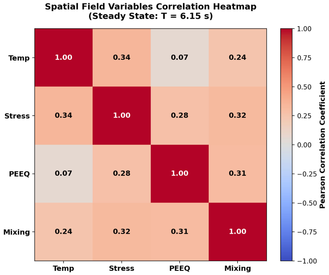
Figure 15.
Principal-component (PCA) loadings for the four thermomechanical fields during the steady stage (t = 6.15 s) of FSW. PC1 (44.7%)—“overall intensity of thermomechanical interaction”; PC2 (23.7%)—antiphase behavior of temperature T and plastic strain PEEQ.
Figure 15.
Principal-component (PCA) loadings for the four thermomechanical fields during the steady stage (t = 6.15 s) of FSW. PC1 (44.7%)—“overall intensity of thermomechanical interaction”; PC2 (23.7%)—antiphase behavior of temperature T and plastic strain PEEQ.
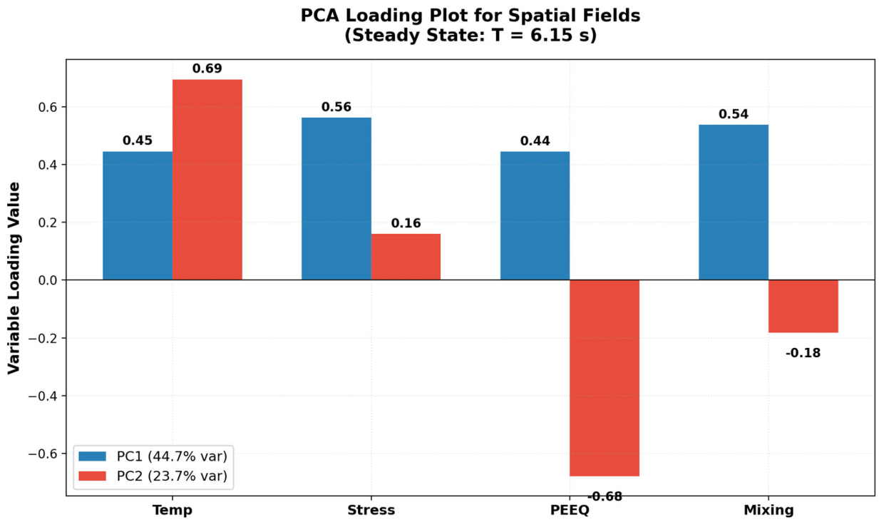

Table 1.
Physical-mechanical, thermophysical, and Johnson–Cook parameters of MA2-1/AZ31B alloy.
| Parameter | Symbol | Value | Units | Source |
| Density | ρ | 1780 | kg/m³ | GOST 14957 |
| Young’s modulus | E | 45 | GPa | [18] |
| Poisson’s ratio | ν | 0.35 | – | [18] |
| Thermal conductivity | λ | 96 | W/(m·K) | [11] |
| Specific heat capacity | cₚ | 1020 | J/(kg·K) | [11] |
| Coefficient of thermal expansion | α | 26·10⁻⁶ | K⁻¹ | [11] |
| Melting temperature | T_melt | 923 | K | [11] |
| JC reference temperature | T_ref | 293 | K | [17] |
| Reference strain rate | ε̇₀ | 0.001 | s⁻¹ | [17] |
| JC: yield stress | A | 172 | MPa | [17] |
| JC: strain-hardening coefficient | B | 361 | MPa | [18] |
| JC: hardening exponent | n | 0.456 | – | [18] |
| JC: strain-rate hardening coefficient | C | 0.092 | – | [18] |
| JC: thermal-softening exponent | m | 0.90 | – | [18] |
Table 2.
Thermal boundary conditions of the CEL model.
| Boundary | Condition type | Parameter | Value |
| Bottom (z = 0) | Convection − backing plate | h_back | 1000 W/(m²·K) |
| Open surfaces | Convection—air | h_air | 20 W/(m²·K) |
| Open surfaces | Radiation | ε | 0.30 |
| Contact Γ_c | Contact thermal conductance | h_contact | 3000 W/(m²·K) |
| Contact Γ_c | Frictional heat flux | q_fric (Eq. 3.13) | – |
| All surfaces | Initial temperature | T₀ | 293 K |
Table 3.
Eulerian-domain mesh parameters.
| Parameter | Pin zone |x|<15 mm | Periphery |x|>15 mm | Buffer z>5.5 mm |
| Element size in X, mm | 0.50 | 1.00 | 1.00 |
| Element size in Z, mm | 0.30 | 0.50 | 1.00 |
| Element size in Y, mm | 0.50 | 1.00 | 1.00 |
| Number of elements, ×1000 | ~120 | ~135 | ~80 |
Table 4.
Computational model parameters and variation ranges used in the parametric study.
| Parameter | Range | Baseline value |
| Shoulder radius R_sh, mm | 6 / 9 / 12 | 9 |
| Pin radius R_pin_bot, mm | 2 / 3 / 4 | 3 |
| Rotational speed ω, rpm | 600 / 800 / 1000 / 1200 | 800 |
| Traverse speed v, mm/min | 60 / 100 / 140 / 180 | 100 |
| Plate thickness h, mm | 3.0 (constant) | 3.0 |
| Z-buffer thickness, mm | 2.5 | 2.5 |
| Friction coefficient μ | 0.4 | 0.4 |
| Plastic dissipation coefficient η | 0.9 | 0.9 |
| Total number of elements, thousands | ~350 | ~350 |
Table 5.
Computational resources and simulation parameters.
| Resource | Characteristic |
| RAM, peak consumption | ~24 GB |
| Disk space (ODB files) | ~18 GB per configuration (32 output frames) |
| Number of processor cores (MPI) | 16 cores, ~3.5 GHz (Intel Xeon) |
| Computational time per configuration | ~8–12 hours |
| Number of configurations (parametric study) | 11 (baseline + 10 variants) |
| Total CPU time | ~110–130 hours (≈ 5–6 days) |
| Software | Abaqus/Explicit 2023 HF4; Python 3.10 (post-processing) |
| Output data format | Abaqus ODB; PNG/CSV export via Abaqus Python API |
Table 6.
Output characteristics for all parametric configurations.
| Configuration | T_peak, °C | σ_mean, MPa | PEEQ_max | W_mix, mm | Leading factor |
| Baseline | 480 | 77.0 | 147 | 5.00 | – |
| R_sh = 6 mm | 379 ↓21% | 123.9 ↑61% | 147 = | 5.00 = | T,σ |
| R_sh = 12 mm | 567 ↑18% | 37.2 ↓52% | 147 = | 5.00 = | T,σ |
| ω = 600 rpm | 425 ↓11% | 98.8 ↑28% | 126 ↓14% | 4.48 ↓10% | T,σ,P,W |
| ω = 1000 rpm | 527 ↑10% | 56.9 ↓26% | 166 ↑13% | 5.44 ↑9% | T,σ,P,W |
| ω = 1200 rpm | 569 ↑19% | 38.1 ↓51% | 184 ↑25% | 5.83 ↑17% | T,σ,P,W |
| v = 60 mm/min | 554 ↑15% | 41.5 ↓46% | 185 ↑26% | 5.68 ↑14% | T,σ,P |
| v = 140 mm/min | 437 ↓9% | 99.6 ↑29% | 126 ↓14% | 4.60 ↓8% | T,σ,P |
| v = 180 mm/min | 407 ↓15% | 116.2 ↑51% | 113 ↓23% | 4.32 ↓14% | T,σ,P |
| R_pin = 2 mm | 470 ↓2% | 81.4 ↑6% | 142 ↓3% | 3.50 ↓30% | W |
| R_pin = 4 mm | 487 ↑1% | 73.8 ↓4% | 150 ↑2% | 6.44 ↑29% | W |
Notes: Arrows and percentages indicate deviation from baseline.
Table 7.
Summary of coefficients and exponents of regression Equations (3.2) − (3.5).
| Equation | Y | C | a₁ (ω) | a₂ (R_sh) | a₃ (R_pin) | a₄ (v) | R² | Main factor |
| (4.2) | T_peak, °C | 27.84 | +0.420 | +0.580 | +0.050 | −0.280 | 1.000 | R_sh > ω > v |
| (4.3) | σ_mean, MPa | 273632 | −1.313 | −1.674 | −0.189 | +0.952 | 0.952 | R_sh > ω > v |
| (4.4) | PEEQ_max | 27.07 | +0.550 | 0.000 | +0.080 | −0.450 | 1.000 | ω > v >> R_pin |
| (4.5) | W_mix, mm | 0.474 | +0.380 | 0.000 | +0.880 | −0.250 | 1.000 | R_pin > ω > v |
Table 8.
Asymmetry coefficients K_asm and weld parameters for the investigated FSW conditions of MA2-1 plates.
Table 8.
Asymmetry coefficients K_asm and weld parameters for the investigated FSW conditions of MA2-1 plates.
| Configuration | K_asm(T) | K_asm(PEEQ) | K_asm(σ) | T_max, °C | W_mix, mm | PEEQ_max |
| Baseline* | 1.08 | 1.25 | 1.18 | ~950 | ~5.0 | ~6.1 |
| R_sh = 6 mm | 1.05 | 1.22 | 1.14 | ~870 | ~4.2 | ~5.8 |
| R_sh = 12 mm | 1.12 | 1.28 | 1.23 | ~1020 | ~6.1 | ~6.4 |
| ω = 600 rpm | 1.04 | 1.15 | 1.10 | ~890 | ~3.8 | ~5.2 |
| ω = 1000 rpm | 1.11 | 1.33 | 1.24 | ~975 | ~5.8 | ~6.5 |
| ω = 1200 rpm | 1.14 | 1.40 | 1.28 | ~1005 | ~6.4 | ~6.8 |
| v = 60 mm/min | 1.10 | 1.30 | 1.21 | ~975 | ~5.6 | ~6.2 |
| v = 140 mm/min | 1.06 | 1.17 | 1.14 | ~930 | ~4.6 | ~5.9 |
| v = 180 mm/min | 1.05 | 1.10 | 1.12 | ~920 | ~4.1 | ~5.6 |
| R_pin_bot = 2 mm | 1.07 | 1.23 | 1.16 | ~940 | ~2.9 | ~5.9 |
| R_pin_bot = 4 mm | 1.09 | 1.27 | 1.20 | ~955 | ~7.3 | ~6.3 |
* Note: baseline—ω = 800 rpm, v = 100 mm/min, R_sh = 9 mm, R_pin = 3 mm.
Disclaimer/Publisher’s Note: The statements, opinions and data contained in all publications are solely those of the individual author(s) and contributor(s) and not of MDPI and/or the editor(s). MDPI and/or the editor(s) disclaim responsibility for any injury to people or property resulting from any ideas, methods, instructions or products referred to in the content. |
© 2026 by the authors. Licensee MDPI, Basel, Switzerland. This article is an open access article distributed under the terms and conditions of the Creative Commons Attribution (CC BY) license.
Copyright: This open access article is published under a Creative Commons CC BY 4.0 license, which permit the free download, distribution, and reuse, provided that the author and preprint are cited in any reuse.