

Submitted:
29 September 2026
Posted:
30 September 2026
You are already at the latest version
Abstract
The Unified Electro-Gravity (UEG) theory, originally developed to self-consistently model a stable structure of the electron, is generalized to model a variety of composite charged as well as neutral particles, which may constitute all known elementary particles in the standard model of particle physics. A direct extension of the UEG theory for the electron is possible by modifying the functional dependence between the electro-gravitational field and the energy density, which would lead to a general class of basic charged particles carrying different levels of mass/energy, with the electron mass at the lowest level. The basic theory may also be extended to model simple composite neutral particles, consisting of two layers of surface charges of equal magnitudes but opposite signs. The model may be similarly generalized to synthesize more complex structures of composite charged or neutral particles, consisting of increasing levels of charged layers. Depending upon its specific basic or composite structure, a particle could be highly stable like an electron or a proton, or relatively unstable in different degrees, which may be identified with other known particles of the standard model of particle physics. The generalized UEG theory would provide a new unified model for particle physics, as a potential new paradigm that would complement and apply beyond the standard model of particle physics currently used.
Keywords:
Unified Electro-Gravity (UEG) Theory
; particle physics
; elementary particles
; beyond standard model
1. Introduction
Recently, a Unified Electro-Gravity (UEG) theory is successfully established in [1] to self-consistently model an ideal “static electron” without spin, which can be extended as well to model a spinning electron [2]. The new UEG theory, in its most basic form, introduces a new gravitational field, referred to as the UEG field, proportional to electromagnetic energy density, with the constant of proportionality referred to as the UEG constant . A sufficiently strong UEG field due to the electrostatic energy density of a charged particle could effectively counter the the charge’s self-repulsive electric force, allowing a self-consistently stable charge structure. The UEG constant, used in the basic analysis is shown in [1,2] to be closely related to the fine-structure constant of electrodynamics [3,4], validated in consistency with Casimir effect [5,6], establishing significant confidence in the basic UEG theory. There is also increasing evidence that the proposed UEG field due to energy density in the stellar light radiation in galaxies, or in the cosmic background radiation, could consistently explain yet unresolved astrophysical phenomena [7,8], potentially providing independent supports for the theory in both small (electron) as well as large large (astrophysical) scales of nature.
The stable solutions in the basic UEG theory of [1,2] include discrete levels of mass/energy, where the lowest possible mass/energy state is recognized as a static electron, and differences between the energy levels are found to be small as compared to the energy of the electron. It is clear that the basic form of the theory [1,2] can neither model a proton, which is another stable charged particle in common occurrence, with significantly larger mass than electron, nor a neutron, which is also in common occurrence but carries a zero total charge, nor many other known charged or neutral particles in the standard model of particle physics. In order that the UEG theory can be established as a truly unified theory, it needs to be generalized for successful application to all known charged or neutral particles.
The basic UEG theory of [1] may be extended by having the UEG field to be dependent on higher powers of the energy density , expressed in terms of a general function referred to as a UEG function. With a suitable form of the UEG function, stable solutions for a charged particle with higher levels of mass/energy would be possible, where a stable solution in the next higher level following the electron maybe identified as a proton. The general UEG function maybe properly approximated, with discrete values of the UEG function for the different levels of the stable solutions. A general UEG model with such a discretized approximation of the general UEG function maybe treated analytically equivalent to a basic UEG model of [1,2] with a fixed UEG constant, by associating different discrete values of the UEG constant to the different levels of stable mass. Accordingly, the derivations and results in the basic UEG model of the electron [1,2] maybe directly applicable to model the higher levels of stable particles, by simply substituting the UEG constant with a specific different value for a different level of stable mass. Consequently, a fundamental dimensionless constant, which relates the UEG constant, the stable mass and the associated classical radius, as established in [1,2] in relation to the fine structure constant, would in principle remain valid for all levels of the stable solutions. This would be a significant development, which would indicate that the UEG theory, to which the dimensionless fine-structure constant may trace its fundamental origin, can be much general in its scope of application to a broad class - possibly all - charged particles, independent of any specific configuration or mass of the particle.
The derivations of the UEG theory of [1,2] may also be extended, with reasonable additional effort, to model a general class of composite neutral particles, consisting of a general internal charge structure which is enclosed by an external layer of charge of equal magnitude but opposite in sign, as compared to the total internal charge. A special class of such neutral particles (the zeroth kind) may be identified as neutrinos, when two oppositely charged layers are very closely spaced, resulting in significantly lower mass of the neutral particles than those associated with their internal charge structure without the external charge layer. A composite neutral particle, made of a negative charge layer that encloses a positively-charged layer of a proton, having the total mass close to that of the proton, maybe identified as a neutron. The mass/energy of any general composite neutral particle may be related to that of the internal charge structure, and values of different critical energies, using simple formulations, based on the results of [1,2]. For a special configuration of the neutral particles (the first kind), the above formulations may need to be numerically solved. In this case, the factor (meson factor) relating the mass of a synthesized neutral particle and that associated with its internal charge structure maybe numerically calculated, that can be tabulated or plotted in a general normalized form for convenient use to model any neutral particle of the special kind.
The above modelings may be extended, formulated in the most general form, to model increasingly complex structures of composite charged or neutral particles. They can be synthesized using multiple charge layers, arranged in multiple levels and sub-levels (shells), and be associated with different orders of stability depending on the specific structure. Such a large class of general particles maybe identified with all known particles in the standard model of particle physics. Depending on the specific charge structure and associated stability, a particle may be identified as a baryon, meson, lepton, or a basic boson, representing all observed particles covered by the standard model of particle physics [9,10,11]. Such a generalized UEG model would provide a new paradigm that may be a substitute for the standard model, making the basic weak and strong forces of the standard model [12,13] in principle redundant. In other words, the electromagnetic and gravitational forces, which were successfully unified through the basic UEG theory of [1,2], could be effectively unified as well with the hypothetical weak and strong forces of particle physics, through the generalization established in the present work. That would be a remarkable development in modern physics.
All the models presented in the paper are explicitly valid for ideal static particles, that do not include spin. The Planck’s constant, which is twice the spin angular momentum of a fermionic (baryon and lepton) particle, should be indirectly related to the UEG constant through their shared relationship with the fine-structure constant, discussed earlier. This may suggest that spin dynamics, described by the Planck’s constant, could be closely related to the UEG theory. Accordingly, the UEG theory could conceivably be extended to dynamic modeling of a spinning particle at any general level, where the central acceleration of the spinning particle would be supported by the UEG effects of the particle’s own electric and magnetic fields. Such an extended dynamic UEG model for general particles maybe separately explored similar to the modeling of a spinning electron in [2], beyond the scope of the present paper. However, for useful mass estimations in this paper, we may simply assume that the total mass/energy of an elementary spinning charge at any given level is about twice that of a static charge at the level without the spin [1,2]. Accordingly, for all calculations in this paper, the mass in a given level maybe assumed to be twice or equal to the UEG static mass [1,2] in the particular level, depending on if the spin contribution in the level is included or not, respectively.
2. A General UEG Theory, with Higher Order Functional Dependence of the UEG Field on Energy Density
The UEG theory of [1] introduces a new gravitational acceleration (called the UEG field) dependent on the conventional electromagnetic energy density . With the required condition , the new UEG field would be zero, and therefore the conventional Newtonian gravitation would be maintained unchanged, in the external region of an electrically neutral body (like a rock, a planet (earth)), consistent with normal observation. The new UEG field is equivalent to modifying the conventional mass/energy distribution, with additional new mass (called UEG mass) distribution defined as the divergence of the vector function .
The basic UEG theory, applicable for the stable structure of an electron, is briefly presented in the Appendix II. This is the essential part of the UEG theory of [1], presented for theoretical completeness and continuity with the following analysis of general particles. In the basic UEG theory of [1], Appendix II, the general UEG field is expressed in its simplest form , as a radial acceleration directly proportional to the energy density , with the proportionality constant . Accordingly, the basic UEG theory and associated results of [1], Appendix II, may be extended for the general UEG theory, by substituting the UEG constant parameter used in [1], Appendix II, with an equivalent general UEG function , to be valid for any general functional dependence of the UEG field, or its associated function , with the energy density . For analytical simplicity, the general UEG function maybe treated with a “stair-case” approximation, having different discrete values of for different ranges of the energy density , or equivalently for different ranges of the electric flux density D, or for corresponding different ranges of the radial distance r, as shown in Figure 1. Like in the basic UEG theory of [1], Appendix II, we may also assume in the general theory that the new UEG field is much stronger than the conventional Newtonian gravitational field, which is equivalent to having the new UEG mass distribution much larger than the conventional mass distribution .
Figure 1.
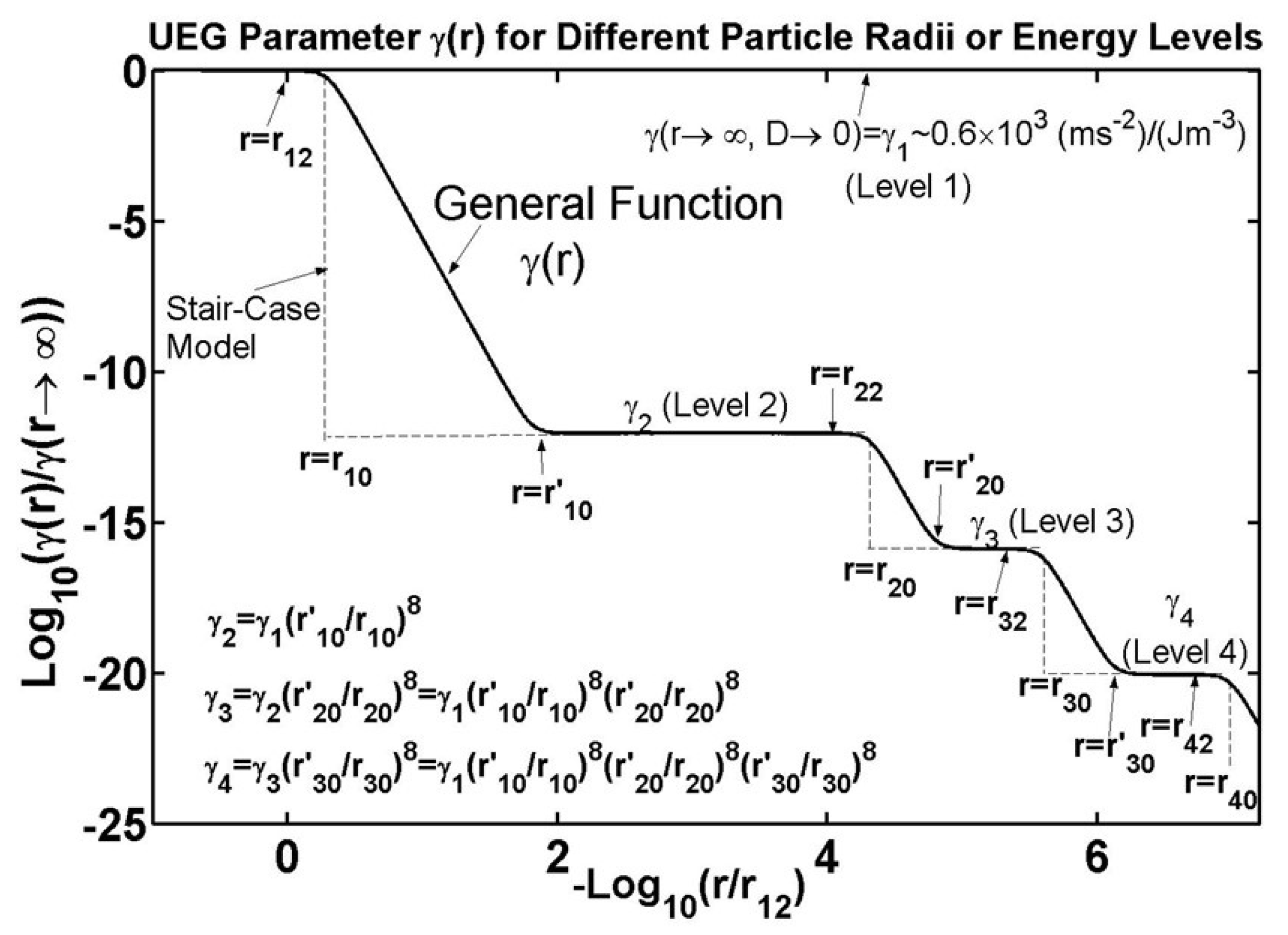
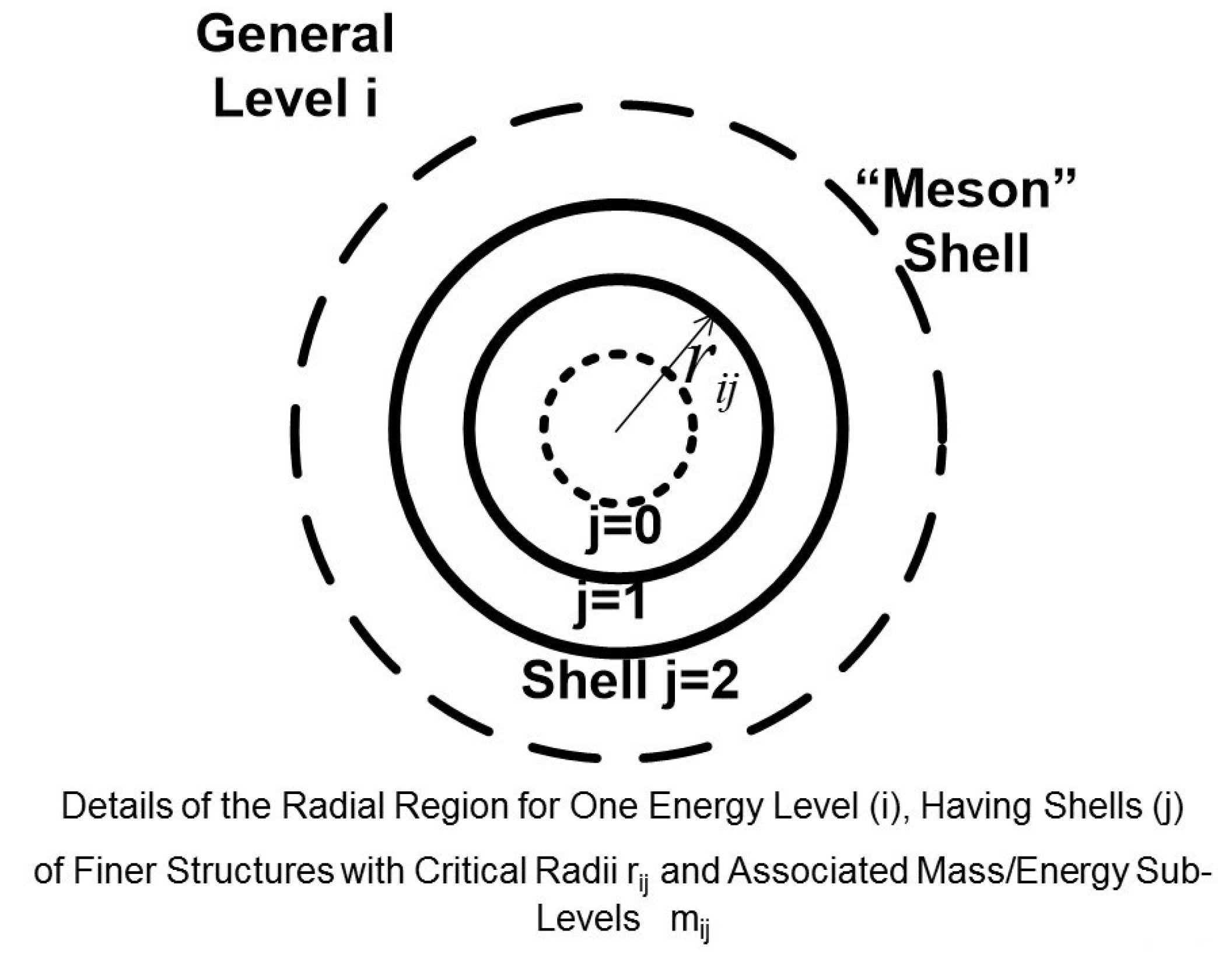
The basic mass (energy) function , which is the total mass (energy) of an elementary spherical charge layer placed at radius r, and the inverse relative-permittivity function which is the inverse of the relative permittivity seen at the charge layer at radius r, maybe derived (see the sketches in Figures 2, 3) using the basic UEG theory of [1] (see equations (A6,A7), Appendix II), based on the stair-case approximation of (3) for the . The radii where the mass function is stable would represent stable elementary charge particles. The mass and radii of such stable charged particles may be indexed as and , respectively, in reference to a particular level i of the general UEG theory, and a particular shell j (= 1, 2) in the given level (see Figures 4, 5).
Figure 2.
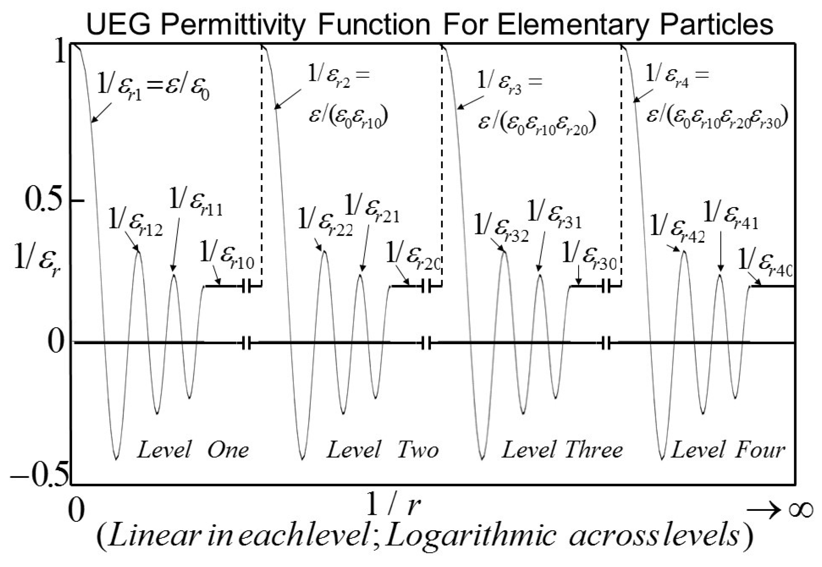
Figure 3.
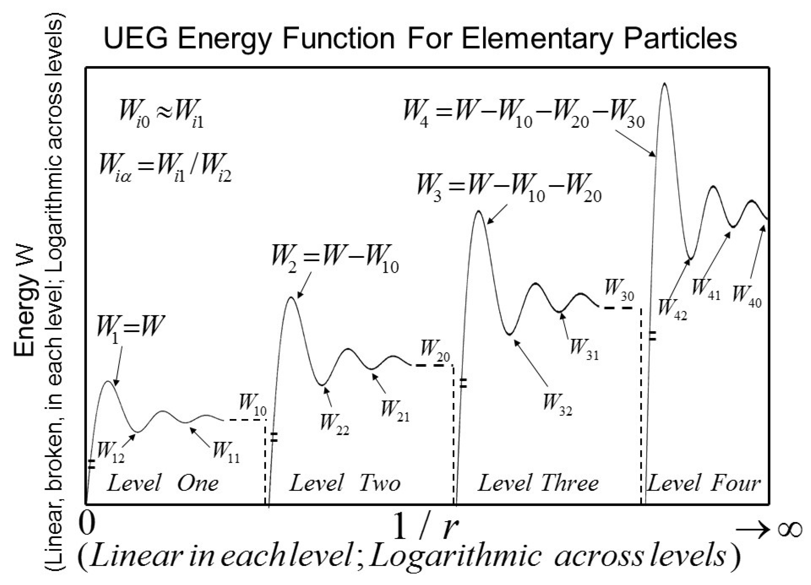
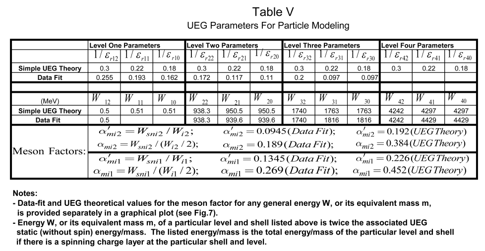
Note that the mass profile in a given level i refers to an ideal derivation in the absence of all levels lower than i, with a fixed UEG constant for the given level that is valid for all r to infinite distance. However, in the presence of a neighboring lower level , the mass associated with the level i needs to be properly truncated at the boundary of the level at , resulting in the effective truncated mass to be valid only for , with an initial condition , and equal to . Therefore, to be particular, any mass , listed in Table V, actually refers to the respective truncated value , which would be exactly and approximately equal to its ideal non-truncated value, respectively for levels 1 and 2, but be somewhat lower than the ideal value for levels 3 and 4.
In addition to the stable elementary charge particles, various kinds of neutral particles that carry zero total charge, as well as various composite charge particles combining the neutral and the stable elementary particles, can be synthesized based on certain basic principles of the UEG theory [1], Appendix II. A basic neutral particle may consist of two elementary charges of opposite signs, placed at two different radii. Alternatively, a neutral particle may consist of an internal composite charge structure surrounded by an external elementary charge layer, with zero total charge. This way a large number of charged or neutral particles could be synthesized from the UEG theory, consisting of all particles (leptons, baryons and mesons) as well as different force carriers (bosons), and possibly even other particles that have not yet been discovered or are not practically realized because suitable decay paths might not be realized in particle-collision experiments. Such particle synthesis using the UEG theory would provide a complete, alternate model to the existing standard model of the particle physics [12,13].
The stability of a neutral or a composite charge particle is determined by the stability of the individual parts of its total structure. Accordingly, such particles may be stable or “quasi-stable” depending on if all or most parts are definitively stable, while any remaining parts are only quasi-stable. The two different kinds of stability of the parts, referred to here, are analogous to having a massive particle on earth placed inside a bowl, or on top of an inverted bowl, where the first kind is definitively stable and the second kind is conditionally stable or quasi-stable. A quasi-stable state would represent a transient state that would decay into stable particles, or other quasi-stable particles that are relatively more stable, having lower total mass/energy. Even a definitively stable particle, with availability of enough energy to overcome its local “energy valley”, may decay into other stable or quasi-stable particles of lower mass/energy. This will determine possible decay paths and associated transient times for the different particles.
Figure 4.
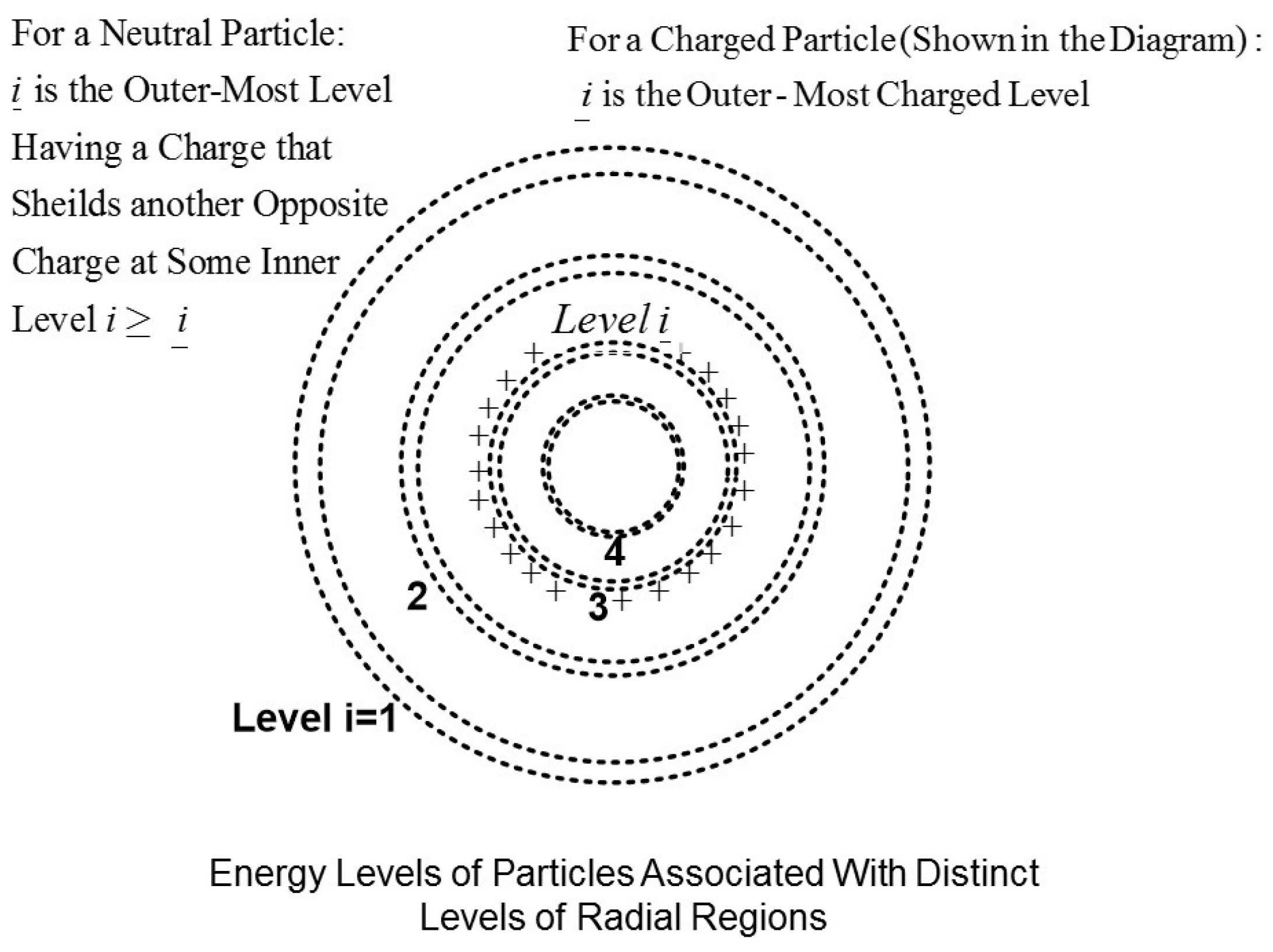
Figure 5.
In the following we will separately discuss the individual types of neutral or composite charge particles.
3. Neutrino: A Neutral Particle of the Zeroth Kind, with Oppositely Charged Layers Close to Each Other.
3.1. Neutrino for the First Level, Based on the Basic UEG Model
We will first consider the basic UEG model, which is applicable to the level one. Similar results can then be extended to the general UEG model as applicable to any higher level.
The inverse-permittivity function (equation (A6), Appendix II) of the basic UEG theory [1] (or a general UEG theory for any higher level, see Figure 2) oscillates around . Given , two layers of opposite charges at radii close to but slightly (infinitesimally) larger than , , would produce a stable synthesized neutral particle having a relatively small, non-zero mass. Such a particle is recognized as an electron neutrino [14,15,16]. The oppositely charge layers in the above configuration, when they are closely spaced around any other radii where would result in a theoretically stable body but with a zero mass/energy. It may be noted, if the two radii and , , are close to each other but both are smaller than , it can be shown to result in a negative, unstable energy. This case is not considered in the following detailed analyses because the resulting negative, unstable energy would not represent any physical particle.
Based on the UEG theory [1], given the mass and the inverse relative-permittivity profiles of an elementary charge particle (equations (A6,A7), Appendix II), the mass of a composite neutral body, synthesized with two elementary charges of opposite signs, placed at radii and , , can be expressed as:
The electric fields due to the two layers of charges of equal magnitude but opposite signs would cancel with each other, resulting in zero total field and its associated energy density, in the external region (). Accordingly, the equivalent mass associated with the energy in the external region, produced due the inner charge layer placed at (without presence of the outer charge layer at ), is first subtracted in (4) from the total mass/energy . Further, the inverse relative-permittivity in the external region of the composite neutral body is assumed to be unity, which needs to be continuous with that in the region between the two charge layers across the external boundary at . Therefore, the original function due to the the inner charge (without presence of the external charge ) needs to be scaled by multiplying it with the factor , in order to obtain the new inverse relative-permittivity function of the composite neutral particle that would be valid in the region between its two charge layers . Consequently, the original energy content () between the two charge layers, as discussed above, also needs to be multiplied by the same factor () in order to find the actual new mass of the composite neutral particle. This is because the mass/energy scales in proportion to the inverse relative permittivity [1], Appendix II.
Now, based on (4), the would be zero as , except when is zero.
An approximate model for the and near may be used, in order to simplify the model for the resulting mass of the synthesized neutral particle, and its derivative with respect to r, from which specific conclusions may be conveniently established. Note that the derivatives of and with radius r, at , are of opposite signs (see Figures 2, 3, equations (A6,A7), Appendix II, [1]), represented by the variables and ; , respectively.
As mentioned earlier, we assume as required or assumed in the above mass formula.
When , the resulting of (6) can be shown to be zero, as anticipated earlier, for all other than , or for all
Following the above case with , only when , , it is a stable point as can be shown from the derivative of the approximate mass expression (6) . Note that when , the stability condition is different from a standard stability condition (having the first derivative of the energy/mass function with respect to the radius equal to zero and the second derivative negative for both the radius variables and ) used elsewhere when . In this case with , we need a positive energy derivative with respect to for larger than the stable point, and a negative derivative with , for less than the stable point (so called, a “V” type of stability).
Consider the limiting case, when the above stable point approaches from the larger side, which is equivalent to having positively approaching zero (). More specifically, we have , and they both approach the same value , but the is closer to zero than the . The limiting stable mass in this case is not necessarily zero, having a range of possible positive values between zero and .
It may also be noted, that the original inverse relative-permittivity , which is unity at , corresponds to a standard light speed . In contrast, the scaled inverse relative-permittivity , valid for between the charges at radii (discussed earlier), is equal to at , which is greater than unity in magnitude, approaching infinity for . The corresponding light speed in this case is larger than the standard light speed , approaching infinity for . Accordingly, the speed limit in the medium between the charges is no longer governed by the standard light speed , but by the new light speed which could approach infinity for . This would allow the charges to spin at speeds greater than , even approaching infinite speed for . This is a remarkable new understanding, which would allow the neutral particle to have a significant, non-zero spin angular momentum (as expected from a fermion), even though the total mass is expected to be relatively small or negligible. Such a particle with a small mass, which could even approach zero, but with a non-zero spin angular momentum , may clearly be identified as an electron neutrino [14,15,16], which is a spin-half particle grouped under leptons in the standard model of particle physics [11,13].
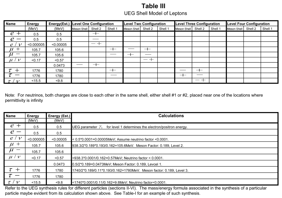
The ratio in (10) maybe estimated based on the and profiles for the level 1 ([1], Figures 2, 3, equations (A6,A7), Appendix II) to be of the order of 5000 eV or so. As per (10), this places only an upper limit, predicting the mass of an electron neutron to be actually any value between zero and about 5000 eV, likely much smaller than the eV limit, as per measured estimates [14]. The upper limit could also be significantly reduced by a more rigorous UEG model. A reference (data-fit) value of 50 eV (= 0.5Mev (electron mass) x 0.0001 (neutron factor)) for this upper limit is adopted in Table III, such that an extension of the UEG theory of the electron neutron to predict similar upper limits for the masses of the muon- and tauon- neutrinos, as presented in the following, would also be consistent with respective measured estimates (see Table III) [14].
3.2. Neutrino at Higher Levels, Based on a General UEG Model
The above neutrino analysis using the basic UEG theory for the level 1, may be similarly extended to a general model applicable to any level. The resulting neutrino in the second and third levels may be identified as the muon and tau neutrinos, respectively [14,17,18]. For such a general model, the basic mass function and inverse-permittivity function in the above analysis maybe substituted by the respective functions and for a particular level i. Accordingly, the final neutrino mass for the level i can be obtained from the mass for the level 1 by simply multiplying by a normalization factor .
() is a useful factor, referred as the neutrino factor, which describes the neutrino mass at a given level as a fraction of the mass of an elementary charge at the respective level.
It may also be noted that in the general higher-order UEG model, for notational and formulational convenience a synthesized neutral mass at any given level i is a standard theoretical mass which assumes that the surrounding external medium has a reference relative permittivity equal to that (=) seen by an elementary charge particle in the level i. This is a hypothetical situation. The actual mass in a practical case, when the external medium is the free space with , would be equal to the standard mass multiplied by the above reference relative permittivity.
4. Neutral Particle of the First Kind, with an External Charge in a “Meson Shell”, and an Internal Oppositely Charged Body Placed at the Same or a Different Level
A neutral particle may be synthesized with opposite charges placed at the same or different levels i and ; . The charge at the inner level may be placed at a shell at a radius , and the opposite charge of the outer level i is placed at a special shell n referred to as the “neutral shell” or “meson shell”, which is different from a regular shell . The name of this special shell is in reference to synthesis of mesons, which often uses this cell to produce relatively lower-mass particles (compared to baryons). Unlike the regular shells that are defined with fixed radii pre-determined as per the basic UEG model, the meson shell radius for the synthesized neutral particle at the level i is a variable determined by the mass of the internal charge particle and masses of all levels . The mass is stable at the radius , determined by having the first derivative of the mass with respect to the radius to be zero and the second derivative positive.
The expression of in (13) is similar in principle to that of in (4), sharing the same basic concepts of the UEG theory of [1], Appendix II. With reference to (13), and Figures 2, 3, equations (A6,A7), Appendix II, [1], for a given the increases, and therefore the numerator of reduces, whereas the factor first remains relatively unchanged but then rapidly increases, as the radius is reduced from closer to the central core of the level i (). As we expected, a minimum (stable) value of the can be clearly established by balancing the two opposing trends indicated above, at a suitable location with outside of the core region, referred to as the “meson shell”.
Note that the standard theoretical value of in (14) needs to be properly scaled using (12), in order to obtain its actual value realized when the external medium is the free space with relative permittivity .
General Neutral Particle of the First Kind, with a Regular or a Composite Charge at an Inner Level:
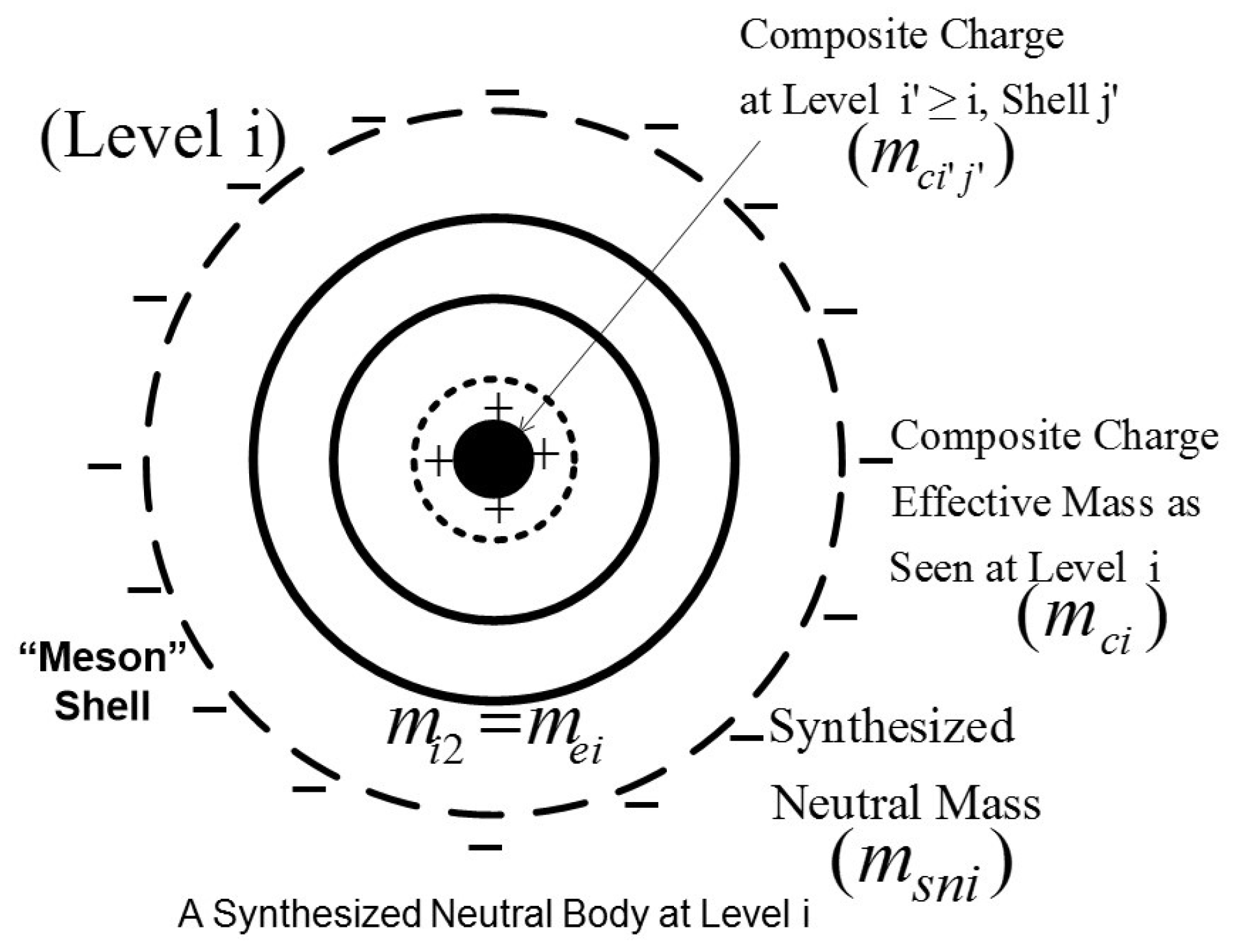
This is a general treatment for the primary kind of neutral particle discussed above. In this case, the inner level charge in the above model maybe substituted by a general charge with effective mass seen at the level i (see Figure 6), which may be a regular charge, or a general composite charge, in the same or different level. If the inner regular or composite charge is stable or quasi-stable without the external opposite charge, it would also be stable/quasi-stable with the external opposite charge. This should be evident from the formula for the synthesized neutral mass .
Figure 6.
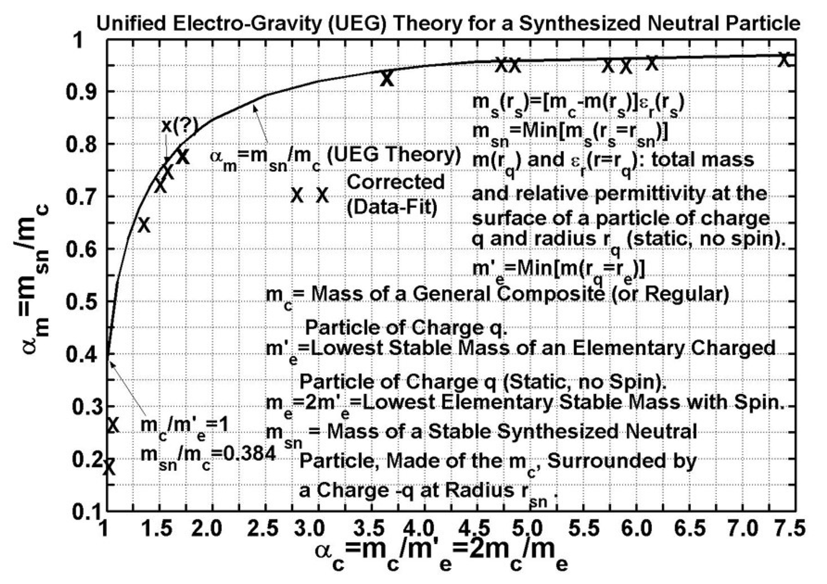
Normalized values for versus are plotted in Figure 7, that maybe applicable for general use at all levels i. These plots are derived using the normalized functions and , which were originally derived from the UEG analysis [1] (equations (A6,A7), Appendix II), for the first level , but are assumed to be approximately valid as well for all levels. This is due to primary similarity of the basic UEG model in all levels. In principle, however, the chart in Figure 7 should be separately established with different best-fit data for each different level. This would accommodate secondary differences in the UEG function , and in the associated mass and inverse-permittivity profiles, in the different levels, as well as differences in any inter-level interactions.
However, for simplicity, we will ignore the secondary deviations between the levels, and instead propose to use the same chart of Figure 7 for all levels. This would be accomplished by simply substituting the ideal non-truncated mass in Figure 7 with the effective truncated mass from Table V (see Section 2, Figure 3), without having to introduce additional truncation parameters for each level. Any resulting deficiency in using the common chart of Figure 7, due to the above non-ideal substitution for a given level, is assumed to be approximately compensated by all the different secondary effects in the level. This appears to be the case, based on the common consistency of all the best-fit data in Figure 7 from different levels.
Figure 7.
5. Neutral Particle of the Second Kind, with the External Charge Placed in a Shell
A second kind of a neutral charge may be synthesized with oppositely charged bodies placed in different levels i and ; . The charged body in the internal level is associated with a shell , as in the first kind of neutral particle (meson, Figure 6) discussed above. However, unlike the first kind of neutral particle, in this case the charge layer in the external level is placed in a conventional shell , not in the “meson shell”. For a special case, if and i maybe the same level, then , which means that the is the internal shell whereas j is the external shell of the common level .
The charged body in the internal level has two possibilities. In the first group, it is a layer of a standard elementary charge of mass , located at radius , with .
The expression of in (17) is similar in principle to that of in (13), and of in (4), sharing the same basic concepts of the UEG theory [1], Appendix II.
General Neutral Particle of the Second Kind, with the External Charge Placed in a Shell :
This is the second group of neutral particles of the second kind, following the first group discussed above. This second group is essentially a general treatment of the first group of particles, by replacing the inner charge layer by a composite charge particle of mass . If the composite charge is stable/quasi-stable without the external opposite charge, the total neutral charge including the external opposite charge would also be stable/quasi-stable.
6. Composite Charged Particles
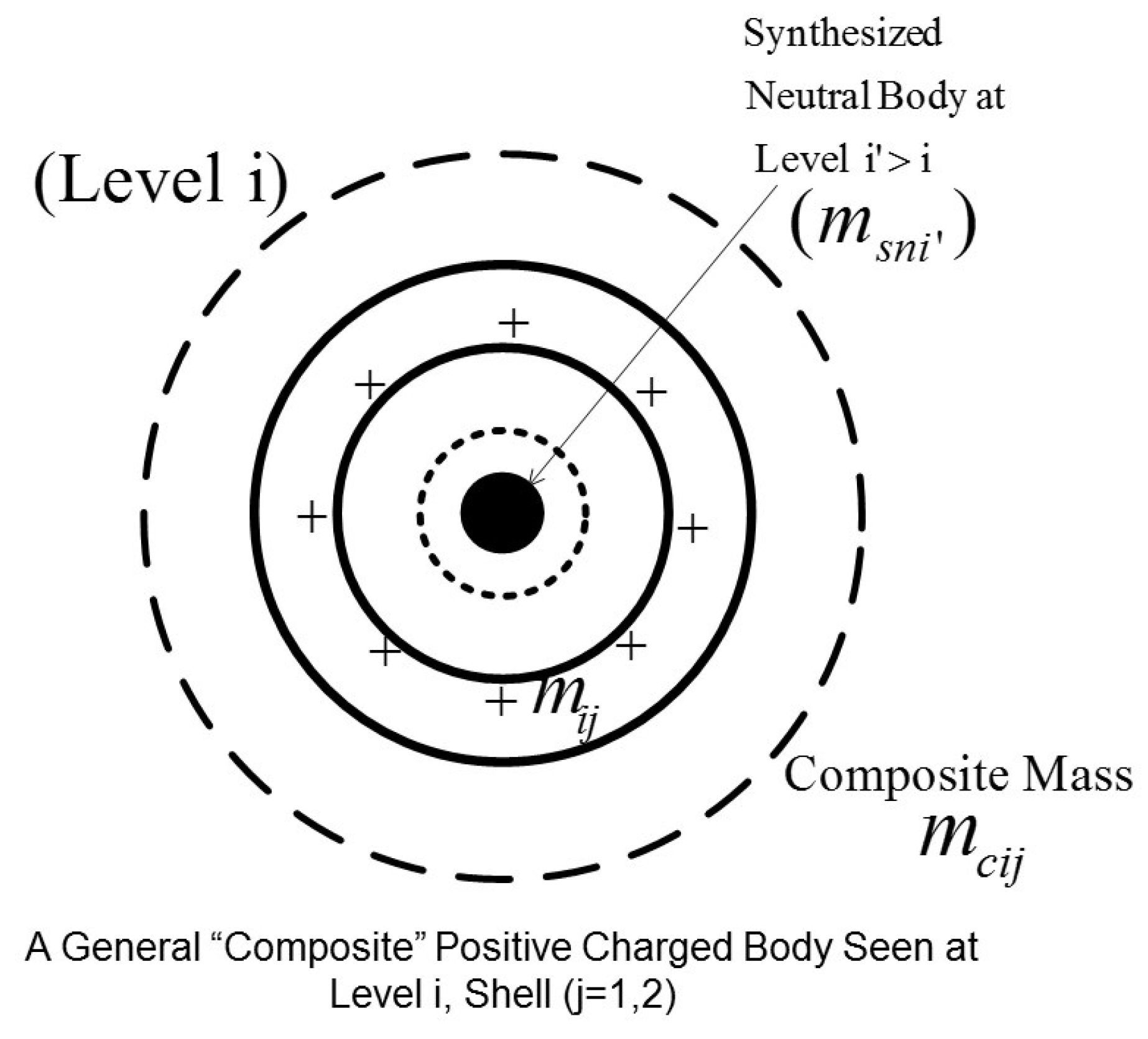
A composite charged particle consists of an elementary charge layer at a radius , at a particular level i and shell j, together with a synthesized neutral particle placed internal to this charged layer at level . The mass or energy of the total particle is quasi-stable at the radius r, defined by the derivative of the mass with the r to be zero, whereas the second derivative may be positive or negative for the part of the mass contributed by the external charge layer or the internal synthesized neutral body, respectively. Due to the quasi-stable nature of the particle, the particle is associated with a transient state that would naturally decay to other particles of lower mass. The mass of such a composite particle may be expressed in terms of the mass of an elementary charge particle at the particular level and shell , with radius , and the mass of the synthesized neutral particle at the level (see Figure 8). The level is normally greater than the level i, but it maybe at the same level as i if the synthesized neutral particle is of the second kind (see Section 5), and the shell of the outermost charge layer of the synthesized neutral particle is internal to the shell j.
It may be noted that, for notational and formulational convenience, the mass or , respectively of an elementary or a composite charged particle at a given level i, refers to only a theoretical number which is the contribution of mass at the given level i and internal to the level. The actual mass, if there is no other charge layer external to the level i, would be equal to this reference theoretical mass plus sum of masses associated with all levels .
Figure 8.
7. Calculations for Known Particles Using the Generalized UEG Theory
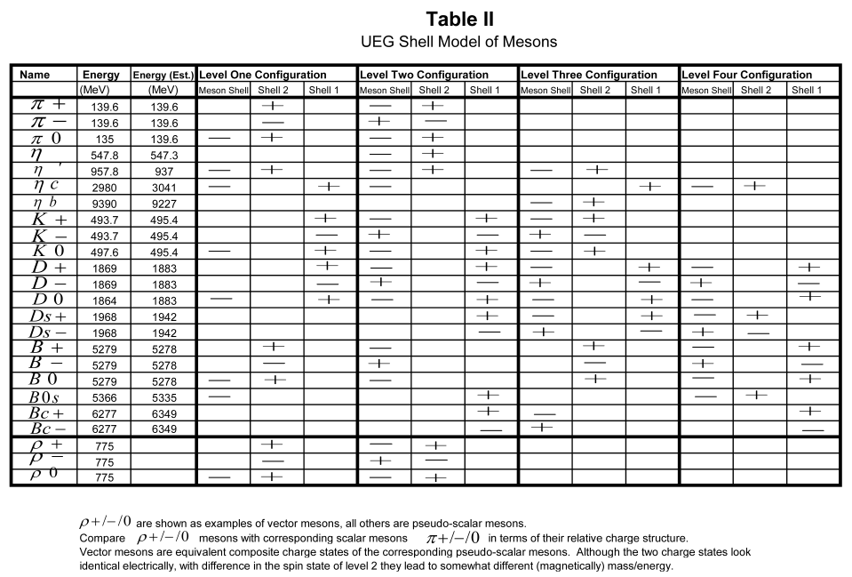
We will apply the generalized UEG theory that we have developed to known particles (leptons, baryons and mesons), and compare the resulting mass/energy estimates from the UEG theory to best available measured values [9,10,11]. The generalized UEG models in Section 3, Section 4, Section 5 and Section 6 are based on a stair-case approximation of the UEG constant in Section 2 for different regions of energy density (see Figure 1), and also assume that the total mass including spin is twice that of the static UEG mass. This ignores any higher-order effects in a rigorous UEG theory, that would require a variable having a smooth functional dependence on the energy density, as well as in a rigorous spin model based on a dynamic UEGM (Unified Electro-Gravito-Magnetic) theory that would be valid for simple as well as composite particles. The rigorous models can be significantly more complicated to compute, and may at this point be pre-mature to establish accurately.
However, the effects of the rigorous models, presumably small over a simplified (first order) general UEG model, may be accounted for by introducing reasonable corrections to various key parameters obtained from the simple UEG theory. The corrected parameters are listed in Table V, and are estimated by fitting the simple UEG theory for selected particles to match their measured mass/energy, as shown in Appendix I. The corresponding parameters obtained from a simple UEG theory are also listed alongside the corrected values in Table V for comparison. The simple and the corrected parameters are seen to maintain certain relative trends from shell to shell in a given particle level, which may imply that the same general foundation is shared by the simple and the rigorous models, except with reasonable numerical adjustments in the parameter values due to higher-order effects.
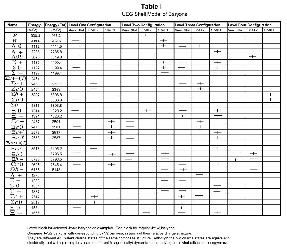
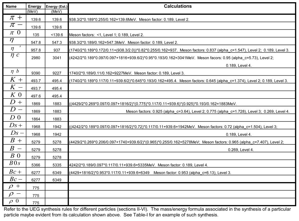
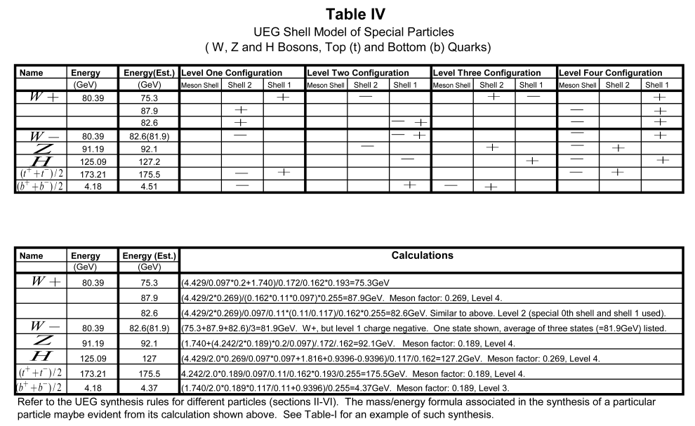
These adjusted parameters from Table V are then used in a simple UEG theory, by employing the synthesis rules of Section 2, Section 3, Section 4, Section 5 and Section 6, to estimate the mass of all leptons (Table I), and all principal baryons (Table II) and mesons (Table III), and the resulting mass estimates are compared to available measured data [9,10,11]. Possible UEG configurations that may emulate other basic particles (Higgs Boson [19,20,21], W and Z bosons [22,23], Top [24,25,26] and Bottom [27,28] quarks) that have been experimentally observed are also listed in Table IV. Note that the Top and Bottom quarks are modeled in the Table IV as equivalent neutral, boson-like particles, which might be detected in pairs that transitionally represent the respective quark-antiquark combinations. Close agreements between the masses estimated using the UEG theory and available measured data in Tables I-IV, for such a large class of basic and composite particles, clearly suggests the power of the new UEG theory as a potential substitute for the Standard Model of particle physics.
It maybe noted, that the spin states assumed for the particles in Tables I-IV, based on the UEG model, may not always match with the expected spin states of the corresponding particles identified from the Standard Model. The correspondence is made based principally on the particles’ charge and mass/energy. That maybe fine, considering that the spin states are often difficult to confirm from measurement, and in such cases they might have been identified in the Standard Model simply based on the model’s (mistaken) theoretical expectations. The measured spin state of a particle, that is based on the spin states of only identified decay products of the particle, might be easily mis-characterized as a meson (boson) instead of a fermion, or vice versa, particularly if a spin-1/2 decay element is missing or improperly detected (a neutrino, for example).
8. Conclusions
The basic UEG theory, first developed to model a static electron [1] and then validated through quantum electrodynamics of a spinning electron [2], is proposed to be generalized in this paper to model all basic and composite particles [9,10,11] covered by the standard model of particle physics. A general structural configuration for a particle, and the associated theoretical and calculation rules to synthesize any such general particle, are proposed and successfully applied to model and predict the masses of a large class of basic and composite particles, including some “force carriers”.
The purpose of the proposed particle configurations and the resulting mass estimates based on the new UEG theory, for such a large class of known particles, is not to focus on any definite study of the individual particles. In fact, it should be reasonable to expect that the actual configurations and mass estimates may deviate somewhat or significantly from those proposed here, almost certainly for a handful of the large number of particles studied. The real purpose is to provide a new theoretical paradigm for particle physics, that is convincingly shown here to have the capacity to model a large class of, possibly all, known basic and composite particles. The clear success of this exercise is a remarkable scientific development. It establishes that the new UEG theory, which obviously unifies the electromagnetic and gravitational theories in explicit terms, could also unify the entire standard model of particle physics [12,13] under its general scope, thus making the strong and weak forces, as well as all classification schemes of elementary particles (leptons, quarks and force carriers), of the standard model in principle redundant. Accordingly, a rigorous version of the new UEG theory may possibly provide a definite physical basis for a grand-unified theory (GUT) [29,30] and a theory of everything (ToE) [31], which have been the grand aspiration of modern physics in recent decades.
Appendix A. Estimation of Parameters of the Unified Electro-Gravity (UEG) Theory, Using Available Energy Data of Known Particles
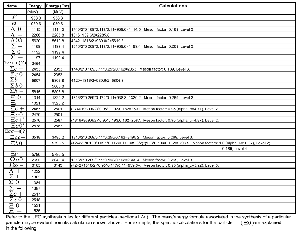
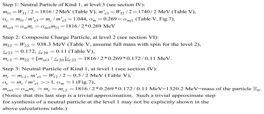
Refer to the UEG synthesis rules for different particles (see sections II-VI). Tables I-IV show the charge structures for all basic and composite particles, synthesized using the UEG theory. The mass/energy formulas associated in the synthesis of the different particles are not explicitly shown, but should be self-evident in the following calculations. For reference, see Table-I for an example calculation of such synthesis.
(1) Electron (e), Proton (p) and Neutron (n), masses determine the energies for levels 1 and 2 :
(2) Use data to calculate and :
(3) Use to calculate :
(4) and energies determine :
(5) , and energies determine . This assumes that the meson factors for both , are approximately the same, because the respective meson mass coefficients are expected to be very close:
(6) Muon mass determines the meson factor for , in level . The result would be valid for all levels i :
(7) Use energy, and from result (4), from result (8b) below, and the factor (see the end note), to get :
(8a) Use energies and the ratio from result (6) to get the ratio :
(8b) Use Tauon energy, and results from (2), (3) and (8a) to calculate and :
(9) , , , and energies determine the energies of level :
(10) Use energies and results from (2), (3), (6) and (8) to get :
The above result assumes . This can now be verified to be correct, because in this case we have .
(11) Use energies and results from (2), (3), (6), (8) and (10) to estimate , which would best-fit with the () meson-factor chart (Figure 7):
Increasing would increase meson coefficient and meson factor , and accordingly the particle mass. We assume that Try first the lowest value for = :
The above calculated mass is reasonably close to the available data for the particle mass =2980MeV, within about a few percent accuracy. Note that the calculation is already larger than the available mass data. Any increase of would increase the particle mass and increase the deviation from the mass data. Therefore, the best estimate for is equal to .
(12) Use energies and results from (2), (3) and (10) to estimate , which would best fit with the () meson-factor chart (Figure 7):
A bit of trial iterations would be needed in the above calculations to get solution for =0.206, (from the chart, Figure 7).
Note: for , for and 4. That is, . Therefore, the corresponding would be same. For this value of , is estimated to be , which best fit all particle data consistent with the UEG theory. Accordingly, we will use for , 4, for all calculations.
Appendix B. A Unified Electro-Gravity Theory, Applied to an Elementary Charged Particle
A Unified Electro-Gravity (UEG) theory is established based on the following basic principles:
(a) The mass m and its associated energy of a given body is assumed to be inversely proportional to the relative permittivity , or directly proportional to the inverse-relative permittivity , of the surrounding medium. This is in consistency with the energy of a spherical surface charge q of radius , placed in a medium with permittivity . The is the permittivity of an “ideal free-space” having an ideal unit relative permittivity , which is assumed to exist far away from any gravitating body .
Using the above concept of mass, a gravitational force at a given location , and its associated field defined as the gravitational force applied on a unit free-mass , may be modeled in terms of the gradient of the inverse-relative permittivity function .
(b) The gravitational field, conventionally defined by the Newton’s Law of gravitation, needs to be modified by adding a new part which is a function of the energy density associated with an electromagnetic field at a given location. As a simple first-order approximation, the new gravitational field , referred to as the UEG field, is assumed to be directly proportional to the energy density, with the proportionality constant referred to as the unified electro-gravity (UEG) constant. The proposed modification would maintain the Newtonian gravitational field as the total field for an electrically-neutral, non-radiating massive body (like planet earth), in the external region where the electromagnetic energy density is zero. It would, however, change the nature of gravitation for an electrically-charged body (like an electron), or a radiating body (like a star or galaxy), where the energy density associated with the electrical charge or light radiation is non-zero. Similarly, it would also change the nature of gravitation in the internal region of an electrically neutral body (like a neutron or neutrino,) which is assumed to consist of internal charged substructures. The modified theory may be alternately interpreted by not modifying the Newton’s Law of gravitation, but re-defining the energy density in an electromagnetic field, such that the total energy/mass of a neutral body remains unchanged.
The modified theory will fundamentally shape the physical structure of any charged particle, such as an electron. The new electro-gravitational field would determine the inverse-relative permittivity function around an electron, as per the relation (A1). We may further assume that the new gravitational field , directed toward the center along , is much stronger than the conventional Newtonian gravitational field, and therefore would essentially be equal to the total gravitational field .
Appendix B.1. Energy Density in a Non-Linear Medium
In the above unified electro-gravity (UEG) model, the permittivity distribution of the free-space is dependent upon the energy density distribution, which is dependent upon the source charge. This is unlike a linear dielectric medium where the permittivity function is independent of the field strength or the source charge. Having the permittivity distribution to be a function of the source charge, is equivalent to having the electric field distribution to be a non-linear function of the source charge. The energy density in such a non-linear medium needs to be properly modeled, using a general expression for the energy density.
The electric field and the electric flux density produced due to a spherical surface charge q of radius , at a distance r from the center of the charge, in the presence of a permittivity distribution , may be expressed using the Coulomb’s Law.
The total energy W and the associated mass of the charge may be calculated by integrating the energy density in its electric field over the spherical volume outside of the charge . The electric field, and the associated energy density, in the spherical region with would be zero. The may be expressed in (A4) in terms of the flux density due to the charge q, and its incremental value due to an incremental change of the charge. This expression of the energy density would be valid for a general non-linear medium, which may be simplified as for a linear medium.
In equivalency to a conventional definition of the energy density for a linear medium, it would be useful to define a new variable for a non-linear medium. The conventional expression of the energy density for a linear medium, with the inverse-permittivity for the linear medium simply substituted by the new equivalent variable , would be valid as well for a non-linear medium.
II.B. Series Solution for the Inverse-Relative Permittivity Function ϵ ̲ r (r ¯)
The inverse-relative permittivity function may be solved by expanding it as power-series of with unknown coefficients , , and then finding the coefficients in order to satisfy the above UEG relation (A5). This would be possible by establishing an iterative process, relating a coefficient with an increasingly higher index i to those with a lower index, starting with the known value for the lowest coefficient . In the limit of large distance r, the would approach unity, fixing the coefficients .
The governing relationship (A5) for would require the series solution with non-zero values of the coefficients only for . Accordingly, the series solution for the may be conveniently expressed as a power series of a normalized variable , with even powers of t. The normalization parameter is to be determined from (A5), which may be shown to be proportional to . We need not present the detailed steps, as prescribed above, to derive the individual coefficients for the series. The final solution for is expressed in (A6), which may simply be substituted in (A5) to verify its validity. The series (A6) may be recognized as the zeroth-order Bessel function .
Appendix B.2. Particle Energy and Mass, as a Function of the Charge Radius
Once the inverse-relative permittivity function is solved, the energy density can be expressed in terms of the using (A4), which can then be integrated over the total volume outside the charge radius (there is no field inside the charge radius) to obtain the total energy or the equivalent mass of the particle.
The charge radius in (A7) is maintained as a general variable (=r). The general mass function in (A7) would also represent the equivalent energy (=) contained in the field external to a sphere of radius r, produced due to the charge placed at any radius less than r.
Figure A1.
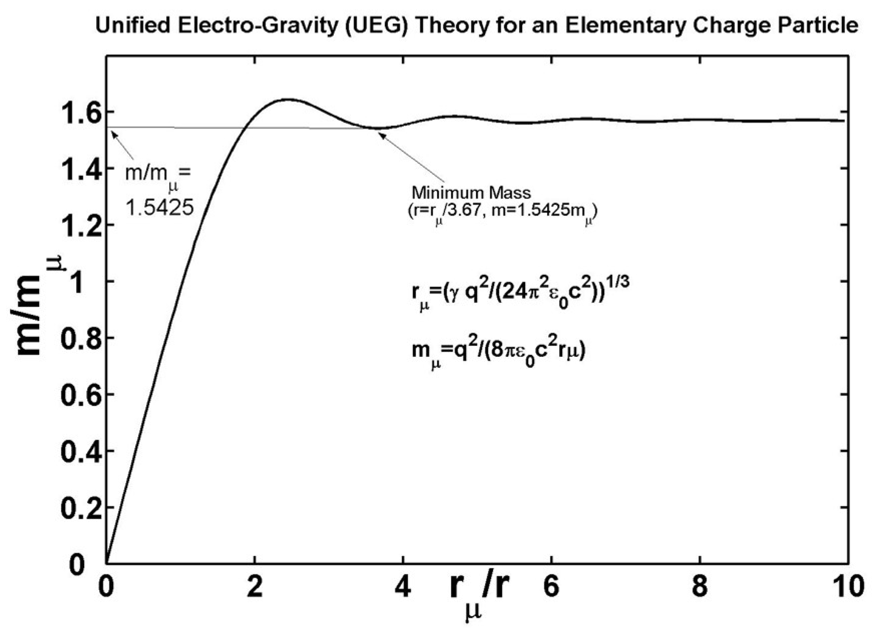
Figure A1 plots the normalized mass of (A7) as a function of the normalized radius , showing an oscillatory behavior of the mass function. Any of the minimum points of the mass function would correspond to a possible stable particle with the particular charge radius .
The smallest possible stable mass deduced from the oscillatory mass of (A7) (Figure A1) is expected to be the mass of an electron (or a positron) without any spin. This is referred to as the static UEG mass of an electron. We will assume that the static UEG mass of an electron is about half of the total electron mass , that includes additional mass/energy due to the electron’s spin. This factor of about 2 between the and is suggested by recognizing that the electron’s spin g-factor is approximately equal to 2. The same conclusion may also be suggested by observing that the orbital magnetic moment of an atomic electron with an orbital angular momentum ℏ is approximately equal to the magnetic moment of a spinning electron with spin angular momentum .
With the assumption of for the minimum stable mass in Figure A1, the value of the normalization constant can be calculated, from which the value of the UEG constant is estimated.
As per the UEG theory of the electron, the constant is declared to be a new natural constant, which is equal to a new gravitational acceleration in toward the center of gravity, produced due to one of energy density.
Appendix B.3. General Relationship Between the UEG Constant γ, the Particle Mass and Classical Radius
The above estimate of the value of the UEG constant is associated the actual value of the UEG static mass of the electron, and carries a specific dimensional unit of . More fundamentally, a dimension-less relationship between the smallest stable UEG static mass of any elementary particle, the corresponding classical radius , and the UEG constant required to produce the mass , can be derived based on the expressions for the reference mass (A7) and reference radius (A6) used in the above analysis.
The value of the ratio from the Figure A1, for the smallest possible stable mass . Using this value, the , and may be related in term of a dimensionless constant.
If we simply assume the total mass of the elementary particle with spin to be twice the UEG mass , and the classical radius associated with half of that () with , the , and may be related using a new dimensionless constant, which would be eight times the above constant.
Notice that the above constant is close to twice the inverse-fine structure constant , and the earlier constant in (A10) is one fourth of the , with less than one percent of difference. The small difference may be due to lack of generality or rigor of the basic UEG static theory for the particle, presented in this paper with assumption of a simple UEG function in (A2), and without including the particle’s spin. The small difference may perhaps be related to the small difference between the actual value of the g-factor and its ideal value of 2 as discussed before. This may point to possible physical origin of the g-factor associated with the spin, governed by a more rigorous version of the new UEG theory.
Leaving aside any small difference due to lack of generality or rigor of the basic UEG model, the close relations of the above dimensionless constant (A10 or A11) to the fine-structure constant is intriguing. The very existence of a dimensionless constant based on the UEG theory, and its intriguing close numerological relationship with the known fine-structure constant , may strongly suggest certain fundamental basis and significance of the new UEG theory. The theory is further validated in [1,2] by successfully modeling the Casimir effect and electron’s spin dynamics, and would be extended in this paper to model other elementary particles in the standard model of particle physics.
References
- Das, N. A New Unified Electro-Gravity Theory for the Electron, and the Fundamental Origin of the Fine Structure Constant and the Casimir Effect. J. High Energy Phys. Gravit. Cosmol. 2021. [Google Scholar] [CrossRef]
- Das, N. A Unified Electro-Gravity Theory of a Spinning Electron, and the Fundamental Origins of the Fine Structure Constant and Quantum Concepts. American Physical Society April 2020 Meeting, Paper ID: Y15.00004 (https://meetings.aps.org/Meeting/APR20/Session/Y15.4), 2020.
- McGregor, M.H. The Power of Alpha (p. 69); World Scientific, 2007.
- Sommerfeld, A. Atomic Structure and Spectral Lines. (Translated by H. L. Brose); Methuen, 1923.
- Casimir, H.B.G. On the Attraction Between Two Perfectly Conducting Plates. Proc. R. Neth. Acad. Arts Sci. 1948, 51, 793–795. [Google Scholar]
- Wikipedia. Casimir Effect. http://en.wikipedia.org/wiki/Casimir_effect, Retrieved, 2019.
- Das, N. A Unified Electro-Gravity Theory to Model Flat Rotation Curves of Spiral Galaxies without Dark Matter. American Astronomical Society 235 Meeting, Paper ID: 444.07 (https://ui.adsabs.harvard.edu/abs/2020AAS...23544407D/abstract), 2020.
- Das, N. A Unified Electro-Gravity Theory to Model Accelerated Expansion of the Universe without any Dark Energy or Dark Matter. American Astronomical Society 237 Meeting (to be presented), Paper ID: 410.02, 2021.
- Wikipedia. List of Baryons. http://en.wikipedia.org/wiki/List_of_baryons, Retrieved, 2013.
- Wikipedia. List of Mesons. http://en.wikipedia.org/wiki/List_of_mesons, Retrieved, 2013.
- Wikipedia. Leptons, Table of Leptons. http://en.wikipedia.org/wiki/Lepton, Retrieved, 2013.
- Schwartz, M.D. Quantun Field Theory and the Standard Model; Cambridge University Press, 2013.
- Cottingham, N.; Greenwood, D. An Introduction to the Standard Model of Particle Physics (2Ed); Cambridge University Press, 2007.
- Wikipedia. Neutrino. http://en.wikipedia.org/wiki/Neutrino, Retrieved, 2017.
- Reines, F. Nobel Lecture: The Neutrino - From Poltergeist to Particle. Nobel Foundation: (Retrieved August 2017) http://www.nobelprize.org/nobel_prizes/physics/laureates/1995/reines-lecture.html, 1995. August.
- Cowan, C. L., Jr.; Reines, F.; Harrison, F.B.; Kruse, H.W. Detection of the Free Neutrino: a Confirmation. Science 1956, 124, 103–104. [Google Scholar] [CrossRef]
- Lederman, L.M. Nobel Lecture: The Neutrino: Observations in Particle Physics from Two Neutrinos to the Standard Model. Nobel Foundation: (Retrieved August 2017) http://www.nobelprize.org/nobel_prizes/physics/laureates/1988/lederman-lecture.html, 1988. August.
- Fermilab. Physicists Find First Direct Evidence of Tau Neutrino at Femilab. (Retrieved August 2017) http://www.fnal.gov/pub/inquiring/physics/neutrino/discovery/index.html, 2000.
- Wikipedia. Higgs Boson. http://en.wikipedia.org/wiki/Higgs_boson, Retrieved, 2017.
- ATLAS Collaboration. Observation of a New Particle in the Search for the Standard Model Higgs Boson with the ATLAS Detector at the LHC. Phys. Lett. B 2012, 716, 1–29. [Google Scholar] [CrossRef]
- CMS Collaboration. Observation of a New Boson at a Mass of 125 Gev with the CMS Experiment at the LHC. Phys. Lett. B 2012, 716, 30–61. [Google Scholar] [CrossRef]
- Wikipedia. W and Z Bosons. http://en.wikipedia.org/wiki/W_and_Z_bosons, Retrieved, 2017.
- CERN Courier. CERN Discoveries: Heavylight. (Retrieved August 2017) http://cern-discoveries.web.cern.ch/cern-discoveries/Courier/Heavylight/Heavylight.html, 1983.
- Wikipedia. Wikipedia. Top Quark. http://en.wikipedia.org/wiki/Top_quark, Retrieved, 2017.
- CDF Collaboration. Observation of Top Quark Prodution in p¯p Collisions with the Collider Detector at Fermilab. Phys. Rev. Lett. 1995, 74, 2626–2631. [Google Scholar] [CrossRef]
- D0 Collaboration. Search for High Mass Top Quark Observation of Top Quark Prodution in pp¯ Collisions at s = 1.8 TeV. Phys. Rev. Lett. 1995, 74, 2422–2426. [Google Scholar] [CrossRef]
- Wikipedia. Bottom Quark. http://en.wikipedia.org/wiki/Bottom_quark, Retrieved, 2017.
- Fermilab. Discoveries at Fermilab: Discovery of the Bottom Quark. (Retrieved August 2017) http://www.fnal.gov/pub/inquiring/physics/discoveries/bottom_quark_pr.html, 1977.
- Georgi, H.; Glashow, S. Unity of All Elementary Particle Forces. Phys. Rev. Lett. 1974, 32, 438–441. [Google Scholar] [CrossRef]
- Pati, J.; Salam, A. Lepton Number as the Fourth Color. Phys. Rev. D. 1974, 10, 275–289. [Google Scholar] [CrossRef]
- Ellis, J. The Superstring: Theory of Everything, or of Nothing. Nature 1986, 323, 595–598. [Google Scholar] [CrossRef]
Disclaimer/Publisher’s Note: The statements, opinions and data contained in all publications are solely those of the individual author(s) and contributor(s) and not of MDPI and/or the editor(s). MDPI and/or the editor(s) disclaim responsibility for any injury to people or property resulting from any ideas, methods, instructions or products referred to in the content. |
© 2026 by the authors. Licensee MDPI, Basel, Switzerland. This article is an open access article distributed under the terms and conditions of the Creative Commons Attribution (CC BY) license (http://creativecommons.org/licenses/by/4.0/).
Copyright: This open access article is published under a Creative Commons CC BY 4.0 license, which permit the free download, distribution, and reuse, provided that the author and preprint are cited in any reuse.