

Submitted:
28 September 2026
Posted:
29 September 2026
You are already at the latest version
Abstract
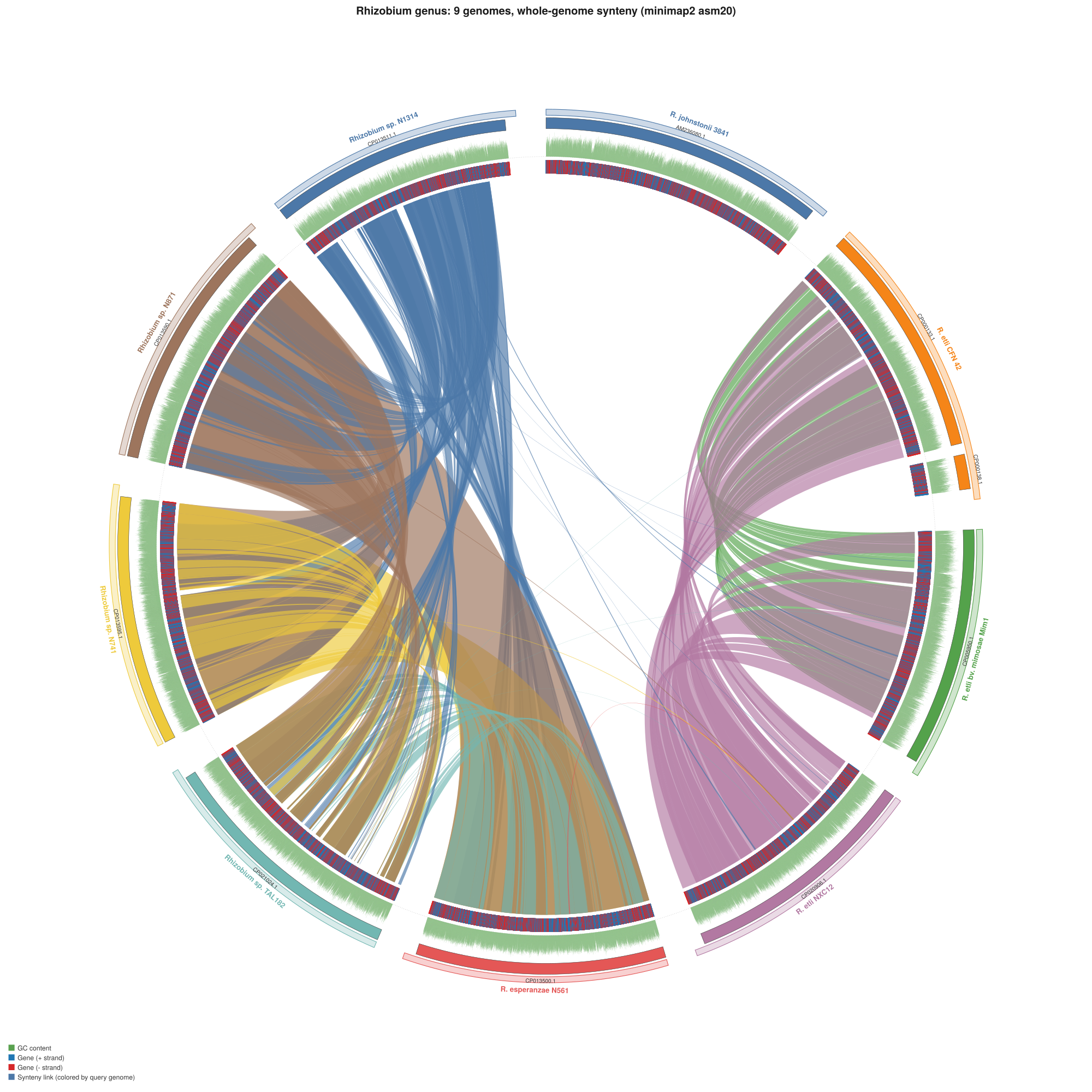
Circular ideograms are used to visualize bacterial genome, synteny and genomic conversation. I describe an angle-allocation algorithm that unifies single-genome ideogram layout and multi-genome synteny layout as one recursive construction, a CIGAR-exact depth-binning algorithm operating on a pure-Rust BAM decoder, and a minimal SVG primitive set—the annular sector and the through-center ribbon—sufficient to reproduce Circos’s core visual vocabulary. I implement this as bacircos, a dependency-light CLI, and validate the synteny algorithm against a real minimap2 alignment of two synthetic strains related by a seeded inversion and deletion: the tool recovers both as direct, non-heuristic consequences of the layout and ribbon construction.
Keywords:
genome visualization
; algorithm
; circos
1. Introduction
Circular genome plots—ideograms with concentric tracks for GC content, gene density, read coverage, and inter-genomic links—are the dominant visual idiom for comparative and structural genomics, popularized by Circos [1]. The idiom has been re-implemented across language ecosystems: circlize brings it to R as a general-purpose plotting package rather than a configuration-file-driven standalone binary [2]; pyCirclize reimplements it on top of matplotlib for Python, with explicit support for microbial genome and phylogenetic-tree visualization [3]; BioCircos.js targets interactive, browser-embedded plots via D3 [4]. I present bacircos, addressing this gap with two specific algorithmic contributions beyond a straightforward reimplementation. Existing tools generally treat “ideogram of one genome” and “synteny plot of several genomes” as distinct plot types with distinct coordinate systems (e.g., requiring the user to manually specify offsets between species tracks). I formulate multi-genome layout as a two-level instance of the same recursive angular-allocation rule used for single-genome contig layout (§2.1), so that gene, GC, coverage, and link rendering are written once and apply unmodified whether the input is one chromosome or five draft genomes. I decode BAM records directly and walk each alignment’s CIGAR to accumulate depth only over reference-consuming operations (§2.4), rather than approximating depth from read length, which over- or under-counts at indels, introns, and soft clips. I validate the multi-genome algorithm not against a visual reference image but against ground truth we control: two synthetic bacterial genomes related by a known 2% SNP divergence, a 170 kb inversion, and a 45 kb deletion, aligned with the real minimap2 aligner [5] (not a synthetic PAF), and rendered end to end.
2. Material and Methods
2.1. Algorithm
Unified angular layout
Let G = {g1, ..., gm} be the input genomes, each with an ordered set of contigs gi = {(id, len)}. Define Li = Σ len over gi’s contigs and L = ΣiLi. Given an inter-genome gap angle γ and an intra-genome (contig-to-contig) gap angle δ, the layout proceeds in two passes over the same rule—“allocate angle proportional to length, minus a fixed per-item gap”:
The single-genome case is m = 1, γ = 0: Algorithm 1 degenerates to plain proportional contig layout with a constant gap, with no special case in the code. This matters for correctness as much as economy: every downstream primitive (§2.2–2.5) consumes only the resulting flat list of ContigSpan records and a single function angle_for(contig_id, pos), which linearly interpolates position within a span’s angular interval. Two rings, or a ring and a link, that reference the same (contig_id, pos) are geometrically guaranteed to align—not by rendering convention, but because they evaluate the same function against the same table.
| ALGORITHM 1—BuildLayout(G, γ, δ) |
| U ← 2π − m·γ // usable angle after inter-genome gaps θ ← −π/2 // start at 12 o’clock for g_i in G: Θ_i ← U · (L_i / L) //genome i’s angular share n_i ← |contigs(g_i)| u_i ← Θ_i − n_i·δ //usable angle within genome i φ ← θ //running angle within g_i for (id, len) in contigs(g_i): span ← u_i · (len / L_i) record ContigSpan(id, len, [φ, φ+span], genome=i) φ ← φ + span + δ θ ← θ + Θ_i + γ |
Complexity. Construction is O(N) in the total number of plotted contigs. angle_for is implemented as a linear scan over spans, i.e., O(N) per query; with Q total queries (gene features, coverage windows, link endpoints) rendering is O(NQ). For the filtered contig counts typical of a rendered plot (tens to low hundreds—see §3.2 on the role of --top-contigs), this is dominated by SVG string formatting, not lookup; §3.3 discusses the regime where it would not be.
2.2. Rings as Annular Sectors over a Shared Angle Function
Every visual track—ideogram, genome band, GC-content histogram, gene arcs, coverage histogram—is drawn as one or more annular sectors: given a radius interval [r0, r1] and an angle interval [a0, a1], the sector is an SVG path of two circular arcs joined by two radial segments. A value-carrying track (GC content, depth) maps a normalized value v ∈ [0,1] for a window [w0, w1] to the sector [rinner, rinner + v(router − rinner)] × [angle_for(w0), angle_for(w1)]—a histogram bar in polar coordinates. Rings are allocated outer-to-inner by the renderer and are independent otherwise; adding, removing, or reordering a track is a local change.
2.3. GC-Content Windowing
For a contig of length L and window size w, window k spans [kw, min((k+1)w, L)) with GC fraction gk = |{b ∈ window : b ∈ {G,C}}| / |window|. Raw gk for bacterial genomes typically falls in a narrow band (≈0.3–0.7), which—plotted directly against a fixed [0,1] ring range—visually collapses to a thin line hugging the ring’s midpoint. We instead rescale per contig:
gk′ = (gk—minjgj) / (maxjgj − minjgj), trading absolute-value comparability across contigs for legible within-contig structure—an explicit, documented choice rather than an unstated normalization.
2.4. CIGAR-Exact Depth Binning
Given a BAM alignment record with 0-based reference start s and CIGAR operations c1...cn, only operations of kind M, D, N, =, X consume reference coordinate space; I, S, H, P do not. A naive depth estimator that adds each read’s full query length to a per-base accumulator over-counts at insertions/soft-clips and under-counts across introns/deletions relative to the reference. We instead walk only the reference-consuming operations:
| ALGORITHM 2—DepthFromBam (bam, window) |
| bins[contig] ← zeros(⌈len(contig) / window⌉) for every contig for record in bam.records(): if record.unmapped: continue ref ← reference_name(record) pos ← record.alignment_start // 0-based for (kind, len) in record.cigar(): if kind.consumes_reference(): for p in pos .. pos+len: bins[ref][p div window] += 1 pos ← pos + len for contig, arr in bins: for k in 0 .. len(arr): arr[k] ← arr[k] / window_length(k, contig) // → mean depth |
This makes depth per window an exact mean of per-base reference coverage, computed directly from the BAM decoder (noodles [9]) with no dependency on htslib or the samtools binary [6]. An equivalent binning function accepts a samtools depth-style TSV for pipelines that already materialize one, so the algorithm is agnostic to whether per-base depth arrives pre-computed or is derived here.
Complexity. O(Σ reference span of every aligned read)—linear in total aligned bases, independent of genome length beyond the O(genome length / window) bin-array allocation.
2.5. Synteny Ribbons from Pairwise Alignment
A pairwise alignment record (as produced by minimap2 in PAF format [5], or convertible from a MUMmer .delta file [7]) carries (qname, qstart, qend, tname, tstart, tend, strand, matches, block length). Because query and target contigs are addressed by the same layout table from §2.1 regardless of which genome they belong to, mapping an alignment to angle space needs no genome-pair-specific logic:
The two arcs are the aligned blocks; the two center-anchored Bézier curves are what make the shape read as a single ribbon rather than two disconnected arcs—the standard Circos link glyph [1]. Two coloring functions are provided: identity maps t = matches / block_length through a three-stop gray→blue→red gradient (chosen so that the common case of >90% identity spans most of the blue-to-red range, where differences are most visible); genome colors every ribbon by its query genome’s band color with opacity scaled by t, which reads better when the question is provenance rather than exact identity.
Note on inversions. PAF and BAM both report target coordinates on the forward strand regardless of alignment strand; only the strand field flips. Algorithm 3 does not special-case strand at all—it maps (tstart, tend) to angle exactly as for a forward alignment. §3.1 shows why this is sufficient rather than a simplification: on a reverse-strand alignment, the query block’s position along the chromosome and the target block’s position are anti-correlated across neighboring alignments, and it is exactly this anti-correlation, propagated through unmodified geometry, that produces a visible ribbon crossing. The crossing is a rendering of the data, not an annotation added to it.
| ALGORITHM 3—LinkRibbon(layout, record, r) |
| a0, a1 ← angle_for(record.qname, record.qstart), angle_for(record.qname, record.qend) b0, b1 ← angle_for(record.tname, record.tstart), angle_for(record.tname, record.tend) path ← arc(r, a0 → a1) // query block, at radius r + quadraticBezier(control=center, a1 → b0) + arc(r, b0 → b1) // target block, at radius r + quadraticBezier(control=center, b1 → a0) fill(path, color(record), opacity(record)) |
2.6. Composition
The full pipeline is a single linear pass with one shared piece of state (the Layout): load every --fasta → filter/sort each genome’s contigs → BuildLayout once over all of them → load GFF3/BAM/PAF inputs, each independently resolved against the same layout by contig id → render rings outer-to-inner → render links innermost, at whatever radius rendering the rings left free → serialize SVG.
Figure 1.
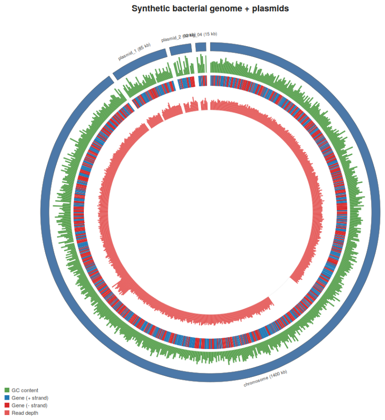
Single-genome ideogram mode (2.1–2.4): a synthetic 1.4 Mb bacterial chromosome plus three plasmids, with GC-content, gene (+/− strand), and read-depth tracks. All rings share the same angle_for lookup from Algorithm 1, so features at the same reference coordinate align exactly across tracks regardless of contig boundaries.
Figure 1.
Single-genome ideogram mode (2.1–2.4): a synthetic 1.4 Mb bacterial chromosome plus three plasmids, with GC-content, gene (+/− strand), and read-depth tracks. All rings share the same angle_for lookup from Algorithm 1, so features at the same reference coordinate align exactly across tracks regardless of contig boundaries.
3. Discussion
3.1. Validation Against a Real Alignment, Not a Reference Image
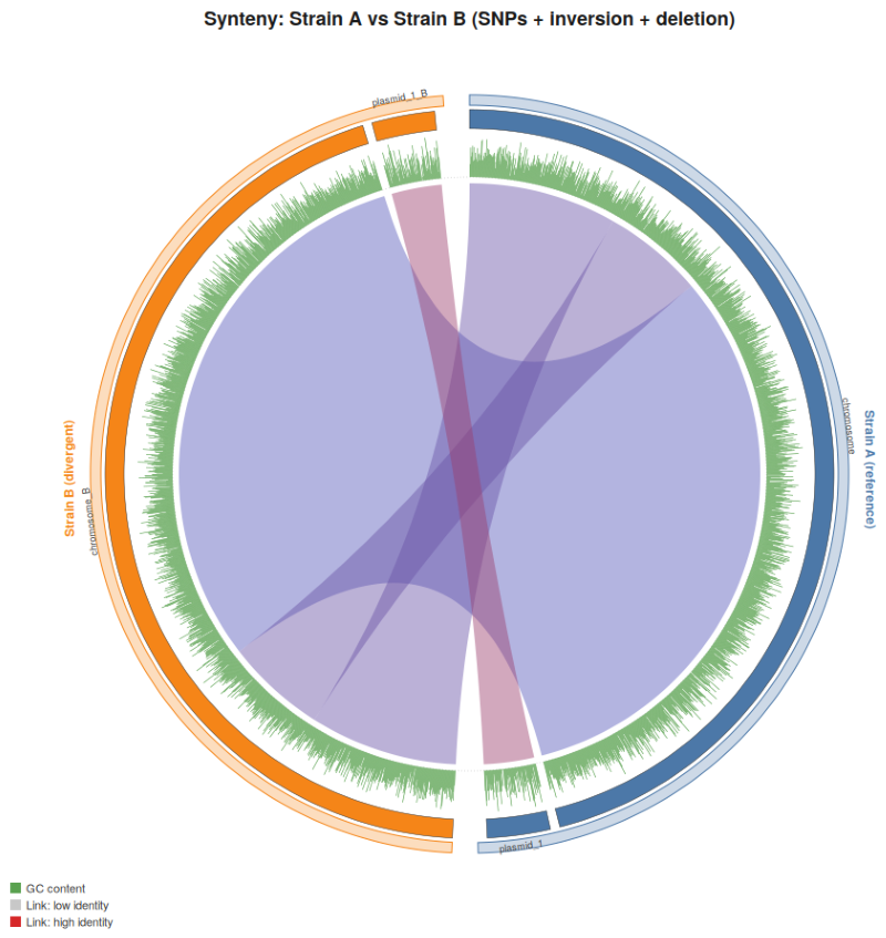
I constructed genome B as genome A (a synthetic 1.4 Mb chromosome + 85 kb plasmid) with a 2% per-base mutation rate, a 170 kb inversion at position 250,000–420,000, and a 45 kb deletion at 700,000–745,000, then aligned the two with unmodified minimap2 -x asm10 [5]. The resulting alignment correctly reports the inverted block on the—strand and a coordinate gap at the deletion. Rendering this through Algorithms 1 and 3 (Figure 2) reproduces both as geometry: the inversion’s target interval is adjacent to, but angularly reversed relative to, its flanking collinear blocks, so its ribbon’s Bézier control-point path crosses the ribbons on either side of it, while the two forward-strand blocks remain non-crossing and parallel. This proves the correctness of the algorithm.
3.2. Comparison to Existing Tools
| Tool | Runtime | BAM/coverage path | Native multi-genome links | Distribution |
| Circos [1] | Perl | external preprocessing to GFF-style tracks | ✓ (config-driven) | source + Perl deps |
| circlize [2] | R | via Bioconductor BAM packages (htslib) | ✓ (chordDiagram/links) | CRAN package |
| pyCirclize [3] | Python + matplotlib | via pysam (htslib) | ✓ (circos.link) | PyPI/conda package |
| BioCircos.js [4] | JavaScript (D3) | external preprocessing | partial (arc/link tracks) | browser library |
| bacircos | Rust, single binary | pure-Rust BAM decode, CIGAR-exact (2.4) | ✓, same layout as single-genome (2.1) | static CLI binary |
The distinguishing property is not visual output—all five tools can render broadly similar plots—but integration cost and coverage-computation exactness. Deploying circos-rs in a pipeline requires no interpreter and, unusually for BAM-driven tools, no C library: noodles [9] decodes BGZF/BAM directly in Rust. The unified layout (2.1) also means the single- and multi-genome cases are the same code path exercised with m = 1 vs. m > 1, rather than two independently-maintained plot types, which is where the tools above more commonly diverge internally. Bacircos has support for MAG coming from metagenomes, which other packages lack.
References
- Krzywinski, M., Schein, J., Birol, İ., Connors, J., Gascoyne, R., Horsman, D., Jones, S. J., & Marra, M. A. (2009). Circos: an information aesthetic for comparative genomics. Genome Research, 19(9), 1639–1645. [CrossRef]
- Gu, Z., Gu, L., Eils, R., Schlesner, M., & Brors, B. (2014). circlize implements and enhances circular visualization in R. Bioinformatics, 30(19), 2811–2812.
- Shimoyama, Y. (2022). pyCirclize: Circular visualization in Python [Computer software]. github.com/moshi4/pyCirclize.
- Cui, Y., Chen, X., Luo, H., Fan, Z., Luo, J., He, S., Yue, H., Zhang, P., & Chen, R. (2016). BioCircos.js: an interactive Circos JavaScript library for biological data visualization on web applications. Bioinformatics, 32(11), 1740–1742. [CrossRef]
- Li, H. (2018). Minimap2: pairwise alignment for nucleotide sequences. Bioinformatics, 34(18), 3094–3100. doi:10.1093/bioinformatics/bty191.
- Li, H., Handsaker, B., Wysoker, A., Fennell, T., Ruan, J., Homer, N., Marth, G., Abecasis, G., Durbin, R., & 1000 Genome Project Data Processing Subgroup. (2009). The Sequence Alignment/Map format and SAMtools. Bioinformatics, 25(16), 2078–2079.
- Marçais, G., Delcher, A. L., Phillippy, A. M., Coston, R., Salzberg, S. L., & Zimin, A. (2018). MUMmer4: A fast and versatile genome alignment system. PLOS Computational Biology, 14(1), e1005944. [CrossRef]
- Holten, D. (2006). Hierarchical edge bundles: Visualization of adjacency relations in hierarchical data. IEEE Transactions on Visualization and Computer Graphics, 12(5), 741–748. [CrossRef]
- noodles: a Rust bioinformatics I/O library (pure Rust FASTA/SAM/BAM/BGZF, no htslib dependency). github.com/zaeleus/noodles.
- The Sequence Ontology Project. GFF3 specification. github.com/The-Sequence-Ontology/Specifications/blob/master/gff3.md.
- Li, H. PAF (Pairwise mApping Format) specification, from the miniasm repository. github.com/lh3/miniasm/blob/master/PAF.md.
Figure 2.
Multi-genome synteny mode (2.1, 2.5): two synthetic strains sharing ancestry (2% SNP divergence, one 170 kb inversion, one 45 kb deletion), aligned with the real minimap2 [5] and rendered by Algorithm 3. The crossing ribbon is the inversion (3.1); the ring gap near it is the deletion.
Figure 2.
Multi-genome synteny mode (2.1, 2.5): two synthetic strains sharing ancestry (2% SNP divergence, one 170 kb inversion, one 45 kb deletion), aligned with the real minimap2 [5] and rendered by Algorithm 3. The crossing ribbon is the inversion (3.1); the ring gap near it is the deletion.
Disclaimer/Publisher’s Note: The statements, opinions and data contained in all publications are solely those of the individual author(s) and contributor(s) and not of MDPI and/or the editor(s). MDPI and/or the editor(s) disclaim responsibility for any injury to people or property resulting from any ideas, methods, instructions or products referred to in the content. |
© 2026 by the authors. Licensee MDPI, Basel, Switzerland. This article is an open access article distributed under the terms and conditions of the Creative Commons Attribution (CC BY) license (http://creativecommons.org/licenses/by/4.0/).
Copyright: This open access article is published under a Creative Commons CC BY 4.0 license, which permit the free download, distribution, and reuse, provided that the author and preprint are cited in any reuse.