
Submitted:
28 September 2026
Posted:
29 September 2026
You are already at the latest version
Abstract
Direction and distance affect both the magnitude and spatial distribution of counts in a compact scintillator array, which makes their simultaneous estimation difficult. We modeled radiation transport and detector response in Geant4 11.3.2 for a 12 × 12 yttrium orthosilicate (YSO) array irradiated by an isotropic 11.6 keV photon point source. The analysis assumes a known emitted exposure. A dual-branch convolutional neural network combined the normalized 12 × 12 response with six global descriptors—the total photon rate, two centroid coordinates, two spatial spreads, and covariance—to estimate a front-hemisphere unit direction vector and the source-to-detector distance. The dataset contained 272 training, 96 validation, and 72 in-dependent test positions. Across three initializations, the full model achieved a polar-angle MAE of 5.16 ± 0.42°, circular azimuth MAE of 13.56 ± 0.85°, three-dimensional directional MAE of 9.68 ± 0.84°, distance MAE of 26.33 ± 1.43 mm, and MAPE of 6.29 ± 0.26%. Shape-only and Global-only ablations showed that the spatial pattern and global statistics contributed different information, and the full model outperformed Random Forest, Extra Trees, and template/k-nearest-neighbor baselines on the same test set. The dominant failure mode was azimuth estimation for far-field sources close to the array normal. These results are lim-ited to the simulated test positions and do not establish real-detector performance or reliable full-angle localization at 1 m.
Keywords:
low-energy photon
; point-source localization
; dual-branch convolutional neural network
; spatial–global feature fusion
; pixelated scintillator array
1. Introduction
Rapid localization of low-energy photon point sources is important in nuclear-facility inspection, contamination surveys, emergency response, and portable radiation measurements. Direction estimates can shorten a search and reduce unnecessary exposure, while distance estimates help with source characterization and measurement planning. Gamma-ray localization systems commonly obtain direction-dependent responses from collimators, coded apertures, Compton imaging, multiple detectors, or free-moving detector platforms [1,2,3,4,5,6]. Although these designs provide rich spatial information, they may require shielding or masks, multiple interactions, or motion-dependent reconstruction.
A pixelated scintillator array is a compact alternative because a single exposure provides both the total response and a two-dimensional count distribution. Previous studies have inferred source direction or interaction position from pixel counts, response centroids, likelihood models, and higher-order spatial features [1,7,8]. Most of these systems either assume a fixed source distance, reconstruct a scene with additional geometric constraints, or address detector-event positioning. Joint estimation of direction and distance from one response of an uncollimated array, particularly at low photon energy, has received less attention.
Convolutional neural networks (CNNs) have been applied to radionuclide identification, mobile-source detection, and directional inference from pixelated radiation measurements [9,10,11]. Their spatial filters can resolve weak patterns across an array, but an image-only model does not explicitly separate response shape from absolute rate. This separation is useful here: normalized shape carries most of the angular information, whereas response per emitted primary is an important distance cue. We therefore encode the normalized array and a small set of interpretable global descriptors in separate branches and fuse the resulting features before regression.
Three effects make the joint problem difficult. Total response varies with both viewing geometry and source distance, so rate alone cannot determine either quantity. Responses at different azimuths also become similar as a source approaches the entrance-face normal, where small count fluctuations can lead to large azimuth errors. Conversely, at 11.6 keV the photon range in air is short enough for unequal paths to the near and far sides of the array to produce a stronger count difference at oblique incidence; this makes the two-dimensional pattern more distinctive, even as the overall response falls rapidly with distance. The estimator must retain the absolute rate without discarding these spatial asymmetries.
To address these challenges, we developed an auditable Geant4 workflow and a dual-branch CNN that combines normalized response shape with six global descriptors: ln(T/Nemitted), μx, μy, σx, σy, and covxy. The method predicts a unit direction vector and log-distance and is evaluated on an independent, staggered multi-distance test grid. Across three initializations, it achieved a three-dimensional directional MAE of 9.68 ± 0.84° and a distance MAE of 26.33 ± 1.43 mm. Ablations and conventional baselines supported the value of spatial–global fusion, while the error analysis identified far-field, near-axis azimuth estimation as the principal limitation. These findings apply only to the sampled positions and prescribed exposure function N(R).
2. Materials and Methods
2.1. Localization Task and Coordinate Definition
The center of the detector array was defined as (0, 0, 0), and the crystals lay in the x–y plane. The entrance face was on the z < 0 side, so its outward normal pointed along −z; the source was restricted to this front hemisphere. Source position was parameterized by distance R, polar angle θ, and azimuth φ. Here, θ = 0° places the source on the outward normal of the entrance face, while φ = atan2(y, x) is mapped to 0°–360°. The angle θ describes the source viewing direction rather than a fixed propagation direction for individual photons, because every primary photon was emitted independently and isotropically into 4π. As θ approaches 0°, directions with different φ values converge in three-dimensional space. We therefore report polar-angle error, circular azimuth error, and the three-dimensional angular separation between predicted and true directions.
2.2. Detector Geometry and Physics Modeling
The production simulation used Geant4 11.3.2 with G4EmStandardPhysics_option4 for electromagnetic interactions and G4OpticalPhysics for scintillation-light transport [12,13,14]. The target energy was selected from the low-energy photon spectrum associated with ²³⁸Pu. This nuclide decays almost entirely by α emission to ²³⁴U, and subsequent atomic relaxation produces uranium L-shell characteristic X rays, including the 11.62 keV Lℓ line [15]. The simulated source therefore emitted one monoenergetic 11.6 keV photon per event. The world volume was an air-filled cube without walls, supports, a human phantom, or environmental background. The detector contained 144 YSO pixels. Each crystal measured 6.0 mm × 6.0 mm × 1.0 mm and was surrounded laterally by a 0.20 mm BaSO₄ reflector and a 0.03 mm aluminum layer. The pixel pitch was 6.66 mm, giving an array envelope of approximately 79.72 mm. A 65 μm enhanced specular reflector (ESR) film covered the entrance face, and a 0.10 mm optical adhesive layer covered the rear face. YSO was defined as Y₂SiO₅ with a density of 4.45 g cm⁻³. Ce activation was represented by empirical scintillation parameters: a yield of 15,300 photons MeV⁻¹ and a decay time of 70 ns [16]. These values are representative modeling inputs rather than measurements from a specific production batch.
YSO(Ce) was selected because its density of 4.45 g cm⁻³ supports efficient photoelectric absorption at 11.6 keV, even with a thin crystal. The yttrium K-edge, approximately 17.0 keV, lies above the incident energy and therefore avoids additional complexity from Y K-shell absorption at the operating point. Its blue scintillation emission is compatible with common photosensors, its decay time is approximately 70 ns, and its non-hygroscopic crystal form is suitable for pixelated-array fabrication [16,17,18,19,20]. These advantages apply to the present model; a hardware study would still need to characterize the actual crystal batch.
Table 1 lists the detector geometry and optical parameters used in the Geant4 model.
The 1.0 mm thickness was selected to reduce interference from the Compton continuum of penetrating background radiation while retaining full-energy deposition at 11.6 keV. It cannot be reduced arbitrarily because mechanical strength and manufacturability must be maintained; greater thickness would lengthen optical-photon paths and could increase interpixel crosstalk. Thus, with the 6.0 mm × 6.0 mm crystal area and 6.66 mm pitch, 1.0 mm is a practical compromise for the present energy and geometry, not a general optimum.
For each pixel, the response was defined as the number of unique optical-photon tracks generated inside a YSO crystal that first crossed from CrystalPixel into the corresponding GluePixel. The 144 counts were arranged by crystal position into a 12 × 12 response matrix. This score is an interface-level optical response in the Geant4 model; it is not a measured SiPM photoelectron count or an electronic analog-to-digital converter output [21,22].
Figure 1 presents the detector geometry and front-hemisphere coordinate system. Figure 1a shows the independently wrapped 12 × 12 pixel array, and Figure 1b defines the point-source position through R, θ, and φ.
Figure 2 shows four representative response heatmaps at φ = 10°, with R = 125 or 925 mm and θ = 25° or 65°. Both distance and polar angle change the total response, hotspot pattern, and centroid, supporting the joint use of absolute response rate and two-dimensional shape to estimate direction and distance.
2.3. Physical Basis of Angular Sensitivity
The array has no coded aperture, collimator, or Compton-imaging structure. Its directional sensitivity arises from changes in the spatial response with source direction. Geometric projection and the solid angle subtended by the finite array change the relative irradiation of individual pixels as (θ, φ) varies, redistributing counts across the 12 × 12 array. Because 11.6 keV photons are attenuated appreciably in air, the different air path lengths to the near and far sides of the array amplify the near-to-far count difference for oblique incidence and make the two-dimensional response more distinctive. Independent wrapping confines most optical response to the corresponding pixel and preserves this spatial contrast. Among 643,548 nonzero-response incident-photon events in the multi-distance scan, 643,546 produced a response in only one pixel, and only two involved two pixels. This finding indicates limited event-level sharing at the present energy and geometry, although it does not demonstrate the absence of self-shielding. Off-axis sources also shift the response centroid and higher-order spatial moments. These effects motivate the low-order moments in the global branch, while the CNN captures higher-order two-dimensional structure.
The same mechanisms limit performance close to the entrance-face normal. As θ approaches 0°, directional pattern differences and centroid displacement diminish, and the response becomes more nearly centrosymmetric. Azimuthal information therefore weakens, making near-normal azimuth estimation less reliable than estimation at larger polar angles. Section 4.2 relates this limitation to the simulated error distribution.
2.4. Data Generation and Integrity Control
Each physical source position produced one accumulated 12 × 12 response matrix together with the complete number of emitted primary particles. Primary events with zero response were omitted from the sparse event rows but remained included in the denominator, Nemitted, thereby preserving the physical meaning of the total photon rate, T/Nemitted. The multi-distance scan recorded 643,548 nonzero-response incident-photon events and 181,576,126 optical photons that entered the adhesive layer. A responding incident photon generated approximately 282 relevant optical photons on average; these correlated optical photons cannot be treated as independent training samples. After conversion, each physical position was stored as one NPZ sample containing source coordinates, R, θ, φ, the 12 × 12 photon_counts matrix, simulated_particles, and the data-split label. A physical source position—not an optical photon—was always the statistical unit for model training and evaluation.
Manifests, random seeds, and configuration identifiers made data generation auditable. Checks covered source coordinates, event counts, pixel indices, duplicate positions across splits, and configuration consistency. Multi-distance positions used distinct, nonrepeating CLHEP random seeds. Because the 20-million-event conversion chunk exceeded the exposure at every position, each position produced one NPZ file and received no additional training weight from chunking.
2.5. Scan Design and Dataset Partitioning
Before the multi-distance scan, we generated a full-azimuth dataset at a fixed distance of R = 300 mm to provide denser angular coverage for the final joint model. This dataset contained 234 physical positions, each simulated with 1.0 million primary photons. The 192 training positions used θ = 10°–80° in 10° increments and φ = 0°–345° in 15° increments. The 24 validation positions used θ ∈ {15°, 35°, 55°, 75°} and six staggered azimuths. An additional 18 positions at R = 300 mm were reserved for diagnostics. In the final multi-distance workflow, all 234 positions were reconverted using one physical position per sample and merged with the multi-distance data. The R = 300 mm samples supplied angular coverage and diagnostics only; they were not treated as independent evidence of distance generalization, and the 18 diagnostic samples were excluded from the primary 72-position test metrics.
The multi-distance scan added 224 multi-distance positions. The 80 training positions used R = 100, 200, 450, 700, and 1000 mm; the 72 validation positions used R = 150, 375, and 850 mm; and the independent held-out test set contained 72 positions at R = 125, 250, 575, and 925 mm. The R, θ, and φ grids were staggered across splits to reduce overlap in sampled positions and coordinate values between splits. Training polar angles ranged from 10° to 80° in 10° increments. Validation used 15°, 35°, 55°, and 75°, whereas testing used 25°, 45°, and 65°. The test azimuths were 10°, 70°, 130°, 190°, 250°, and 310°.
The number of primary events at each position increased approximately with the square of distance according to
Exposure was rounded upward in increments of 0.1 million events. The multi-distance dataset contained 8.108 × 10⁸ primary photons, and all 224 positions passed the integrity audit. After merging with the 234 fixed-R angular positions, the complete dataset comprised 458 physical positions: 272 for training, 96 for validation, and 90 for testing. Only the 72 newly generated held-out positions were used for the principal performance statistics; the 18 diagnostic positions at R = 300 mm were excluded. Figure 3 shows the R–θ scan grid and the θ–φ–R distribution of the 72-position held-out test set.

Table 2.
Multi-distance scan design.
| Dataset | R (mm) | θ | φ | Positions |
|---|---|---|---|---|
| Training | 100, 200, 450, 700, 1000 | 10°–80° in 10° increments | Two phase-shifted reference azimuths at each R | 80 |
| Validation | 150, 375, 850 | 15°, 35°, 55°, 75° | 5°, 65°, 125°, 185°, 245°, 305° | 72 |
| Held-out test | 125, 250, 575, 925 | 25°, 45°, 65° | 10°, 70°, 130°, 190°, 250°, 310° | 72 |
2.6. Dual-Branch CNN with Spatial–Global Feature Fusion
The proposed model performs joint direction–distance regression through two branches followed by spatial–global feature fusion. Let Cij denote the count in pixel (i, j), and let T = Σi,j Cij be the total response. The normalized spatial probability was
The spatial branch received a 3 × 12 × 12 tensor. Its first channel applied the square-root variance-stabilizing transform
and the other two channels were fixed x- and y-coordinate grids. This separation removed total response amplitude from the spatial branch while retaining relative spatial distribution, absolute pixel position, and finite-count noise. Total response was combined instead with centroid, spread, and covariance in a six-dimensional global feature vector,
The global branch used ln(T/Nemitted), the centroid coordinates μx and μy, the spreads σx and σy, and the covariance covxy. Thus, the six descriptors comprised one normalized total-response term and five spatial moments. Nemitted served only as the denominator in T/Nemitted and was not passed to the network as an independent feature. The network therefore had no direct access to the simulated particle count, which was correlated with distance through the exposure schedule.
The spatial branch used Conv 3→16, Conv 16→16, 2 × 2 max pooling, Conv 16→32, Conv 32→32, and adaptive average pooling to 3 × 3. The resulting 288 features were flattened and compressed by Linear 288→64. The global branch used Linear 6→24→24 with SiLU activation. After concatenation, the 88-dimensional vector passed through Linear 88→64, SiLU, and 0.10 dropout. Separate 64→3 and 64→1 heads predicted direction and distance. The complete network contained 41,876 trainable parameters.
The direction target was the unit vector
This representation avoids the 0°/360° azimuth discontinuity [23,24]. The total loss was the equally weighted sum L = Ldir + Lθ + Lφ + LR. Here, Ldir = 1 − û · u constrained the three-dimensional direction, Lφ = 1 − cos(φ̂ − φ) respected azimuthal periodicity, and normalized Smooth-L1 losses were applied to θ and ln(R). Training used AdamW [25] with a learning rate of 0.002, weight decay of 1 × 10⁻⁴, batch size of 32, a maximum of 500 epochs, and early-stopping patience of 100 epochs. Only the training set used random C4 rotations of the square array and inverse-frequency sampling with replacement to approximately balance the training distances. No augmentation was applied to the validation or test set.
Figure 4 summarizes the architecture. The upper path is the CNN spatial branch, the lower path is the six-feature multilayer perceptron (MLP), and the fused representation feeds the direction and distance heads.
Table 3.
Main layers and output dimensions of the dual-branch CNN with spatial–global feature fusion.
Table 3.
Main layers and output dimensions of the dual-branch CNN with spatial–global feature fusion.
| Module | Layer/operation | Output | Role |
|---|---|---|---|
| Spatial input | √(144pij) plus x/y coordinate maps | 3 × 12 × 12 | Preserve normalized spatial shape and absolute pixel position |
| Spatial branch | Conv 3→16→16 + MaxPool | 16 × 6 × 6 | Extract lower-order local spatial features |
| Spatial branch | Conv 16→32→32 | 32 × 6 × 6 | Extract higher-order spatial structure |
| Spatial branch | AdaptiveAvgPool(3 × 3) + Flatten | 288 | Fix the spatial feature dimension |
| Spatial branch | Linear 288→64 + SiLU | 64 | Compress the spatial representation |
| Global branch | Linear 6→24→24 + SiLU | 24 | Encode total rate and low-order moments |
| Fusion | Concat 64 + 24; Linear 88→64 | 64 | Fuse spatial and global information |
| Output heads | Direction 64→3; distance 64→1 | 3 + 1 | Predict the unit direction vector and ln(R) |
2.7. Ablation Design
To separate the contributions of the two input classes, we compared the full model with two single-branch variants. Shape-only retained the 3 × 12 × 12 normalized spatial input and the same CNN backbone but received none of T, Nemitted, the centroid, the spreads, or the covariance. Global-only received the six global physical features and used a 6→24→24→64 MLP for joint regression, without the two-dimensional response matrix. All models used the same 272/96/72 position split, AdamW optimizer, learning rate, joint loss, distance-balanced sampling, validation-based selection, and seeds 2026, 2027, and 2028. The full and Shape-only models used C4 augmentation during training; Global-only had no image input and therefore did not.
The ablations were specified after the first inspection of the test results and should therefore be regarded as exploratory. The mean ± standard deviation (SD) over three seeds reflects sensitivity to network initialization; it is not an estimate of variation among independent physical measurements.
2.8. Conventional and Machine-Learning Baselines
Random Forest [26], Extra Trees [27], and template/kNN implemented with scikit-learn [28] were evaluated after the initial test as baselines for joint localization at unknown distance. Each method used the same 272 training, 96 validation, and 72 held-out test positions as the final network. The test set was not used to select any hyperparameter, distance weight, or neighbor count. Random Forest and Extra Trees received the same six-dimensional input as the Global-only MLP—ln(T/Nemitted), μx, μy, σx, σy, and covxy—and jointly regressed [ux, uy, uz, ln(R)]. The number of trees, maximum depth, minimum leaf size, and max_features were selected using validation data only.
Template/kNN combined the normalized 12 × 12 spatial shape with ln(T/Nemitted). The joint distance between a query and a training template was D = αDshape + βDrate, where Dshape was cosine distance and Drate was the absolute difference in ln(T/Nemitted). The validation-selected configuration was α = 0.8, β = 0.2, and k = 7, with inverse joint distance used as the neighbor weight. The selected Random Forest, Extra Trees, and template/kNN configurations had validation scores of 0.489614, 0.438236, and 0.697233, respectively. The common score was defined as polar-angle MAE/90 + azimuth MAE/180 + mean absolute log-distance error. Because these baselines were added after the initial test result was reviewed, they provide a comparison on the same test set rather than an independent confirmatory test.
2.9. Evaluation Metrics and Analysis Protocol
The evaluation metrics were the MAE of θ, circular MAE of φ, three-dimensional directional MAE, distance MAE, and mean absolute percentage error (MAPE). The circular azimuth error was [29]
Three-dimensional directional error was the spherical angle between predicted and true unit vectors. Validation results are descriptive because they informed early stopping and model selection; none of the 72 test positions was used for either. Seed 2026 was specified in advance for the primary held-out evaluation, whereas seeds 2027 and 2028 were later added to assess initialization sensitivity. Ablations, baselines, test-time augmentation (TTA), fusion, and exposure analyses were also conducted after the initial test results were reviewed. Thus, the reported SD across neural-network seeds measures initialization sensitivity, not confidence intervals or independent Monte Carlo or physical variation.
3. Results
3.1. Primary Held-Out Test Results
The prespecified seed-2026 run achieved a polar-angle MAE of 4.70°, circular azimuth MAE of 12.59°, three-dimensional directional MAE of 8.75°, distance MAE of 24.70 mm, and distance MAPE of 6.00% across the 72 held-out test positions. The three-dimensional directional MAEs at 125, 250, 575, and 925 mm were 4.06°, 4.71°, 12.24°, and 14.01°, respectively, while the corresponding azimuth MAEs increased from 4.46° and 5.37° to 13.69° and 26.83°. Under the current distance-adaptive exposure protocol and test grid, increasing distance affected azimuth and three-dimensional direction more strongly than distance MAPE. Grouping by polar angle yielded azimuth MAEs of 23.17°, 7.79°, and 6.81° at θ = 25°, 45°, and 65°, respectively, showing that azimuthal information was harder to extract near the detector normal.
Figure 5 compares the seed-2026 predictions with the reference values for θ and R and shows the overall circular-azimuth-error distribution. Figure 6 combines the distance-wise metrics with azimuth MAE grouped by true polar angle. Direction errors were low at 125 and 250 mm and increased at 575 and 925 mm, whereas distance MAPE showed no equally strong monotonic deterioration. The much larger azimuth error at θ = 25° is consistent with the expected loss of azimuthal information near the entrance-face normal.
Table 4.
Seed-2026 results by distance for the 72-position held-out test set.
| R (mm) | Positions | θ MAE (°) | φ MAE (°) | 3D MAE (°) | R MAE (mm) | R MAPE (%) |
|---|---|---|---|---|---|---|
| 125 | 18 | 2.40 | 4.46 | 4.06 | 9.69 | 7.75 |
| 250 | 18 | 2.81 | 5.37 | 4.71 | 14.85 | 5.94 |
| 575 | 18 | 8.08 | 13.69 | 12.24 | 34.56 | 6.01 |
| 925 | 18 | 5.50 | 26.83 | 14.01 | 39.68 | 4.29 |
| Overall | 72 | 4.70 | 12.59 | 8.75 | 24.70 | 6.00 |
3.2. Dual-Branch Ablation
The full, Shape-only, and Global-only models were each trained from three random initializations with the same data split, optimizer, joint loss, distance-balanced sampler, and validation-based selection protocol. As shown in Table 5, the full dual-branch model had the lowest value for every overall metric: polar-angle MAE, 5.161 ± 0.422°; circular azimuth MAE, 13.558 ± 0.853°; three-dimensional directional MAE, 9.679 ± 0.838°; distance MAE, 26.333 ± 1.432 mm; and MAPE, 6.288 ± 0.262%.
When the global physical features were removed, Shape-only distance MAE increased to 104.501 ± 17.122 mm and MAPE to 20.392 ± 2.801%; at 925 mm, its distance MAE was 247.012 ± 71.315 mm. The global branch added 2304 parameters (approximately 5.82% relative to Shape-only) but lowered the overall distance MAE by 74.8% and the three-dimensional directional MAE by 22.9%. The size of this change, relative to the modest increase in parameter count, indicates that response rate and low-order moments supplied useful distance information.
Using only six physical features, Global-only achieved a distance MAE of 34.110 ± 3.285 mm and outperformed Shape-only in distance estimation. Its three-dimensional directional MAE was 12.506 ± 0.861°, compared with 9.679 ± 0.838° for the full model, and its P95 was 38.119 ± 4.324°, compared with 25.200 ± 0.827°. The global features therefore captured strong distance information and part of the directional signal but could not replace higher-order structure in the two-dimensional response. Fusion reduced both mean and tail errors at difficult positions. Because a single-branch model was comparable or slightly better in some polar-angle subgroups, the full model was not uniformly superior under every local condition.
3.3. Comparison with Conventional Baselines
Validation data alone determined the hyperparameters of Random Forest, Extra Trees, and template/kNN under the same 272/96/72 position split. Table 6 reports performance on the 72 test positions. Among the conventional baselines, Extra Trees had the lowest polar-angle and three-dimensional directional MAEs, at 11.390° and 29.524°. Random Forest had the lowest circular azimuth MAE (45.720°), while template/kNN had the lowest distance MAE (47.785 mm). No conventional baseline was best across all metrics.
The full dual-branch CNN achieved a three-dimensional directional MAE of 9.679 ± 0.838° and a distance MAE of 26.333 ± 1.432 mm, with corresponding P95 values of 25.200 ± 0.827° and 75.247 ± 7.986 mm. Relative to the best conventional baseline for each metric, the numerical reductions in polar-angle MAE, azimuth MAE, three-dimensional directional MAE, distance MAE, and distance MAPE were 54.7%, 70.3%, 67.2%, 44.9%, and 52.8%, respectively; the three-dimensional directional and distance P95 values were 66.4% and 39.8% lower. Each conventional model used a fixed random_state of 2026, whereas the neural-network values summarize three initialization seeds. Because the comparison was post hoc, these numerical differences should not be interpreted as formal evidence of statistical significance.
Global-only provides a direct comparison with Random Forest and Extra Trees because all three methods used the same six features. Its three-dimensional directional MAE of 12.506 ± 0.861° and distance MAE of 34.110 ± 3.285 mm were lower than those of either tree ensemble. For this dataset and the validation-selected settings, the multi-output MLP described the coupled direction–distance mapping more accurately, and the spatial branch reduced both mean and tail errors further. Template/kNN used response shape together with absolute rate and achieved the lowest conventional distance MAE, but its three-dimensional directional MAE was 41.378°. Its fixed metric and local averaging were poorly matched to directional variation on the sparse multi-distance grid. Figure 7 compares the methods using the two main joint-localization metrics.
3.4. Sensitivity to Initialization and Performance Across the Test Domain
Across three seeds, the mean ± sample SD was 5.16 ± 0.42° for polar-angle MAE, 13.56 ± 0.85° for circular azimuth MAE, 9.68 ± 0.84° for three-dimensional directional MAE, 26.33 ± 1.43 mm for distance MAE, and 6.29 ± 0.26% for MAPE. Large far-field, near-axis errors occurred in every run, so the pattern was not attributable to one unfavorable initialization. Because all runs used the same Monte Carlo test positions, the SDs in Table 7 describe initialization sensitivity, not confidence intervals from independent measurements.
Across the sampled distance–angle grid under the prescribed N(R) exposure schedule, aggregate errors were low at the held-out distances of 125 and 250 mm. Errors were higher at the validation distance of 375 mm and the held-out distance of 575 mm, and large azimuth errors occurred at both the validation distance of 850 mm and the test distance of 925 mm. Validation-distance results are descriptive because they informed model selection. At 925 mm, performance varied with angle: for the θ = 25° subgroup, the three models had azimuth MAEs of 57.31°, 70.34°, and 59.89°, whereas errors at 45° and 65° were much smaller. Thus, the results describe the sampled distances and viewing angles, not a viewing-angle-independent maximum range or continuous cutoff.
Figure 8 shows the three-dimensional directional error at every physical test position for the four held-out distances. Large errors occurred more often at 575 and 925 mm, but they also depended strongly on azimuth. Performance should therefore be interpreted over the sampled angle–distance grid rather than as a function of distance alone.
3.5. Exposure Sensitivity and Post-Processing Analysis
Figure 9 reports an exploratory exposure-sensitivity test on the six positions at R = 925 mm and θ = 25°, selected after the initial errors had been inspected. The original 9.6 million primaries per position defined the 1× condition; independent simulations were then added to obtain 2× and 4× exposure without retraining the models. Mean azimuth MAE across the three models decreased from 62.51° at 1× to 29.28° at 2× and 21.71° at 4×. At 4×, each position contained 38.4 million primaries, and the azimuth MAEs for seeds 2026, 2027, and 2028 were 21.14°, 23.81°, and 20.18°, respectively. Thus, limited response statistics contributed to this failure region. Because the subset was chosen after the failure was observed, the result cannot be generalized to every far-field angle.
Figure 10 compares the post-processing methods. Four-rotation TTA increased azimuth MAE from 12.59° to 13.17°. CNN–centroid complex-vector fusion, weighted using the validation set, reduced the 72-position azimuth MAE only from 12.5866° to 12.4775° and increased the maximum error from 134.71° to 178.28°. The centroid-only method had a similar overall azimuth MAE of 12.45°, but its maximum error reached 162.28°. Similar mean errors therefore masked substantial differences at the weakest-signal positions, and neither simple ensembling nor linear fusion resolved near-axis azimuth instability.
4. Discussion
4.1. Effect of Spatial–Global Feature Fusion and Comparison with Baselines
The ablations indicate that the improvement did not come from a single input class. Shape-only preserved useful directional information, but its distance MAE increased to 104.50 mm. Global-only reduced the distance MAE to 34.11 mm, although its three-dimensional directional MAE and P95 remained at 12.51° and 38.12°. With both branches, these directional errors fell to 9.68° and 25.20°, and the distance MAE was 26.33 mm. The normalized response supplied higher-order spatial structure, whereas total rate, centroid, spread, and covariance supplied complementary global constraints.
The conventional baselines place these errors in context. Using the same 272/96/72 split and validation-selected hyperparameters, their best three-dimensional directional MAE was 29.52° and their best distance MAE was 47.79 mm; the corresponding full-model values were 9.68° and 26.33 mm. The full model also had smaller tail errors. Global-only, despite using the same six inputs as the tree ensembles, gave lower direction and distance errors, while template/kNN represented the directional structure poorly despite using both shape and rate. The comparison is nevertheless exploratory: the baselines were added after the initial test, and each conventional method used one fixed random state. It should not be read as a formal claim of superiority over all conventional methods.
The fixed-distance angular samples at R = 300 mm outnumbered those at any other training distance. We therefore used inverse-frequency sampling with replacement to give the available distances approximately equal weight during optimization and applied 0°, 90°, 180°, and 270° C4 rotations consistent with square-array symmetry. The ablation shows complementarity between the spatial and global input classes, but it did not separately remove distance-balanced sampling or C4 augmentation or isolate each component of the six-feature vector. The gain cannot yet be assigned to one training strategy or individual feature.
4.2. Near-Axis Errors, Exposure Dependence, and Test-Domain Interpretation
The far-field near-axis azimuth error has both geometric and statistical sources. At small θ, the normalized response approaches centrosymmetry and the centroid magnitude approaches zero, making azimuth ill-conditioned. Pixel-level fluctuations can then produce a large change in φ. The improvement at 925 mm and 25° after 4× exposure is consistent with finite response statistics obscuring the spatial asymmetry, although model bias and unfavorable azimuths may also matter. Because optical photons generated by the same incident photon are correlated, the number of responding incident-photon events is a more meaningful measure of effective statistics than the raw optical-photon count.
Performance across the test domain depends directly on the exposure protocol. The multi-distance scan increased N(R) approximately in proportion to R2, so distances were not compared under the same activity–acquisition-time condition. This design examines identifiability after approximate compensation for geometric attenuation, but it does not define a practical acquisition strategy because R is not known before deployment. Future experiments should independently scan distance, θ, and φ under fixed exposure, fixed acquisition time, and several activity levels. Such experiments could map performance across the full three-dimensional domain and define reliability thresholds or calibrated uncertainty estimates from response statistics.
Distance estimation fundamentally depends on known exposure. The global branch uses ln(T/Nemitted) as a distance-related feature. In simulation, Nemitted is known exactly. In a real measurement, expected emitted photons must be inferred from source activity, acquisition time, and the target-line emission probability. If activity or emission probability is unknown, absolute rate and distance have a scale ambiguity and distance is not identifiable. A network can still return a numerical value, but it would lack a reliable physical basis. A practical system should propagate exposure uncertainty into the distance estimate or predict direction alone, a relative distance class, or activity and distance jointly. The distance errors reported here therefore apply only when effective emitted exposure is available.
4.3. Limitations and the Simulation-to-Experiment Gap
Important differences remain between the simulation and a physical detector. The model omitted pixel-to-pixel gain variation, dark counts, electronic thresholds, dead time, pile-up, environmental background, and defective channels; it also idealized YSO, the ESR film, the lateral reflector, the optical adhesive, and the photosensor response. A real system must infer effective emitted exposure from source activity, acquisition time, and target-line emission probability, with uncertainty in each quantity. Because the distance estimator uses absolute response rate, any global efficiency bias will produce a systematic distance error. Hardware implementation therefore requires relative-gain calibration of all 144 channels, conversion of the modeled optical response to photoelectrons and electronic signals, models of background and environmental scatter, and physical-position tests independent of the simulation [21,22]. Domain randomization provides one possible route for broadening simulation variability before hardware transfer [30], but it cannot replace experimental calibration and validation.
The present study used a single isotropic 11.6 keV point source and did not examine other energies, radionuclides, multiple sources, or continuous spectra. Angles and distances were sampled on discrete grids, and the 850 mm results are descriptive because those data were used for validation. Multi-seed retraining, ablation, baseline comparisons, TTA, fusion, and the 2×/4× exposure analysis were all performed after the first review of the held-out results. The tree models used one fixed random state, while the neural-network seeds shared the same 72 physical positions; neither design replaces independent Monte Carlo replications or formal statistical testing. The model also did not provide calibrated epistemic or aleatoric uncertainty. The study therefore evaluates a simulation method and its failure modes, not hardware performance or a 1 m operating limit.
5. Conclusions
We developed a Geant4-based method for joint direction and distance estimation of an 11.6 keV photon point source with a 12 × 12 YSO array. For a known emitted exposure, the 41,876-parameter network combined normalized spatial shape with total photon rate, centroid, spread, and covariance. On 72 held-out positions, the prespecified seed-2026 model achieved a polar-angle MAE of 4.70°, circular azimuth MAE of 12.59°, three-dimensional directional MAE of 8.75°, distance MAE of 24.70 mm, and MAPE of 6.00%. Across three initializations, the corresponding values were 5.16 ± 0.42°, 13.56 ± 0.85°, 9.68 ± 0.84°, 26.33 ± 1.43 mm, and 6.29 ± 0.26%.
The exploratory ablations confirmed that the two input classes were complementary. Removing the global features increased distance MAE from 26.33 to 104.50 mm. Global features alone retained useful distance information, but their three-dimensional directional MAE and P95 were 12.51° and 38.12°, compared with 9.68° and 25.20° for the full model. On the same test set, Extra Trees gave the best conventional three-dimensional directional MAE (29.52°), and template/kNN gave the best conventional distance MAE (47.79 mm); the full-model values were 9.68° and 26.33 mm. These findings apply to the simulated task. Far-field near-axis azimuth remained the main weakness, and every distance result depended on known exposure normalization and the prescribed N(R) schedule. Independent Monte Carlo replications, calibration of a physical SiPM array, and hardware measurements are needed before the method can be assigned a practical operating range.
Author Contributions
Software, Y.L.; writing—original draft preparation, Y.L.; supervision, J.Z. and Y.Y.; methodology and supervision, Q.D. All authors have read and agreed to the published version of the manuscript.
Funding
This research received no external funding.
Institutional Review Board Statement
Not applicable. This study was based entirely on simulation and did not involve humans, animals, or clinical data.
Informed Consent Statement
Not applicable.
Data Availability Statement
The simulation data and code supporting the findings of this study are available from the corresponding author upon reasonable request.
Conflicts of Interest
The authors declare no conflicts of interest.
Abbreviations
| Abbreviation | Definition |
| CNN | Convolutional neural network |
| ESR | Enhanced specular reflector |
| MAE | Mean absolute error |
| MAPE | Mean absolute percentage error |
| MLP | Multilayer perceptron |
| P95 | 95th percentile |
| SiPM | Silicon photomultiplier |
| TTA | Test-time augmentation |
| YSO(Ce) | Cerium-doped yttrium orthosilicate |
References
- Zhao, Q.; Wang, Z.; Li, L.; Li, X.; Zhao, C.; Zhao, M.; Li, F.; Cheng, M.; Zhu, B.; Zhou, R.; et al. A two-dimensional array detector for determining the direction to gamma-ray source. Nucl. Instrum. Methods Phys. Res. A 2022, 1040, 166985. [CrossRef]
- Vetter, K.; Barnowski, R.; Haefner, A.; Joshi, T.H.Y.; Pavlovsky, R.; Quiter, B.J. Gamma-ray imaging for nuclear security and safety: Towards 3-D gamma-ray vision. Nucl. Instrum. Methods Phys. Res. A 2018, 878, 159–168. [CrossRef]
- Al Hamrashdi, H.; Monk, S.D.; Cheneler, D. Passive gamma-ray and neutron imaging systems for national security and nuclear non-proliferation in controlled and uncontrolled detection areas: Review of past and current status. Sensors 2019, 19, 2638. [CrossRef]
- Hellfeld, D.; Bandstra, M.S.; Vavrek, J.R.; Gunter, D.L.; Curtis, J.C.; Salathe, M.; et al. Free-moving quantitative gamma-ray imaging. Sci. Rep. 2021, 11, 20515. [CrossRef]
- Haefner, A.; Barnowski, R.; Luke, P.; Amman, M.; Vetter, K. Handheld real-time volumetric 3-D gamma-ray imaging. Nucl. Instrum. Methods Phys. Res. A 2017, 857, 42–49. [CrossRef]
- Hellfeld, D.; Barton, P.; Gunter, D.; Haefner, A.; Mihailescu, L.; Vetter, K. Real-time free-moving active coded mask 3D gamma-ray imaging. IEEE Trans. Nucl. Sci. 2019, 66, 2252–2260. [CrossRef]
- Shi, R.; Chen, Y.; Dang, X.; Wei, M. Experimental evaluation of reconstruction algorithms for scintillation crystal array based on charge projection readout. Nucl. Instrum. Methods Phys. Res. A 2019, 937, 117–124. [CrossRef]
- Lerche, C.W.; Salomon, A.; Goldschmidt, B.; Lodomez, S.; Weissler, B.; Solf, T. Maximum likelihood positioning and energy correction for scintillation detectors. Phys. Med. Biol. 2016, 61, 1650–1676. [CrossRef]
- Lavelle, C.M.; Miller, E.C.; Ribaudo, C.; Drenkow, N.; Mattson, J. Directional pixelated gamma-ray spectrometer utilizing convolutional neural network and simulated training data. IEEE Trans. Nucl. Sci. 2025, 72, 1602–1611. [CrossRef]
- Daniel, G.; Ceraudo, F.; Limousin, O.; Maier, D.; Meuris, A. Automatic and real-time identification of radionuclides in gamma-ray spectra: A new method based on a convolutional neural network trained with a synthetic data set. IEEE Trans. Nucl. Sci. 2020, 67, 644–653. [CrossRef]
- Bilton, K.J.; Joshi, T.H.Y.; Bandstra, M.S.; Curtis, J.C.; Hellfeld, D.; Vetter, K. Neural network approaches for mobile spectroscopic gamma-ray source detection. J. Nucl. Eng. 2021, 2, 190–206. [CrossRef]
- Basaglia, T.; Bell, Z.W.; D’Agostino, D.; Dressendorfer, P.V.; Giani, S.; Pia, M.G.; Saracco, P. Geant4: A game changer in high energy physics and related applicative fields. Future Gener. Comput. Syst. 2024, 159, 411–422. [CrossRef]
- Allison, J.; Amako, K.; Apostolakis, J.; Arce, P.; Asai, M.; Aso, T.; Bagli, E.; Bagulya, A.; Banerjee, S.; Barrand, G.; et al. Recent developments in Geant4. Nucl. Instrum. Methods Phys. Res. A 2016, 835, 186–225. [CrossRef]
- Dietz-Laursonn, E. Peculiarities in the simulation of optical physics with Geant4. arXiv 2016, arXiv:1612.05162. [CrossRef]
- Chechev, V.P. The evaluation of 238Pu, 240Pu, and 242Pu decay data. AIP Conf. Proc. 2005, 769, 91–94. [CrossRef]
- Chewpraditkul, W.; Wanarak, C.; Szczesniak, T.; et al. Comparison of absorption, luminescence and scintillation characteristics in Lu1.95Y0.05SiO5:Ce,Ca and Y2SiO5:Ce scintillators. Opt. Mater. 2013, 35, 1679–1684. [CrossRef]
- Knoll, G.F. Radiation Detection and Measurement, 4th ed.; John Wiley & Sons: Hoboken, NJ, USA, 2010; ISBN 978-0-470-13148-0.
- Nikl, M. Scintillation detectors for X-rays. Meas. Sci. Technol. 2006, 17, R37–R54. [CrossRef]
- Dujardin, C.; Auffray, E.; Bourret-Courchesne, E.; Dorenbos, P.; Lecoq, P.; Nikl, M.; Vasil’ev, A.N.; Yoshikawa, A.; Zhu, R.-Y. Needs, trends, and advances in inorganic scintillators. IEEE Trans. Nucl. Sci. 2018, 65, 1977–1997. [CrossRef]
- van Eijk, C.W.E. Inorganic scintillators in medical imaging. Phys. Med. Biol. 2002, 47, R85–R106. [CrossRef]
- Piemonte, C.; Gola, A. Overview on the main parameters and technology of modern silicon photomultipliers. Nucl. Instrum. Methods Phys. Res. A 2019, 926, 2–15. [CrossRef]
- Acerbi, F.; Gundacker, S. Understanding and simulating SiPMs. Nucl. Instrum. Methods Phys. Res. A 2019, 926, 16–35. [CrossRef]
- Hara, K.; Vemulapalli, R.; Chellappa, R. Designing deep convolutional neural networks for continuous object orientation estimation. arXiv 2017, arXiv:1702.01499. [CrossRef]
- Prokudin, S.; Gehler, P.; Nowozin, S. Deep directional statistics: Pose estimation with uncertainty quantification. In Computer Vision—ECCV 2018; Springer: Cham, Switzerland, 2018; Volume 11213, pp. 542–559. [CrossRef]
- Loshchilov, I.; Hutter, F. Decoupled weight decay regularization. In Proceedings of the 7th International Conference on Learning Representations (ICLR), New Orleans, LA, USA, 6–9 May 2019; arXiv:1711.05101. [CrossRef]
- Breiman, L. Random forests. Mach. Learn. 2001, 45, 5–32. [CrossRef]
- Geurts, P.; Ernst, D.; Wehenkel, L. Extremely randomized trees. Mach. Learn. 2006, 63, 3–42. [CrossRef]
- Pedregosa, F.; Varoquaux, G.; Gramfort, A.; Michel, V.; Thirion, B.; Grisel, O.; Blondel, M.; Prettenhofer, P.; Weiss, R.; Dubourg, V.; et al. Scikit-learn: Machine learning in Python. J. Mach. Learn. Res. 2011, 12, 2825–2830.
- Pewsey, A.; Neuhäuser, M.; Ruxton, G.D. Circular Statistics in R; Oxford University Press: Oxford, UK, 2013; ISBN 978-0-19-967113-7.
- Tobin, J.; Fong, R.; Ray, A.; Schneider, J.; Zaremba, W.; Abbeel, P. Domain randomization for transferring deep neural networks from simulation to the real world. In Proceedings of the 2017 IEEE/RSJ International Conference on Intelligent Robots and Systems (IROS), Vancouver, BC, Canada, 24–28 September 2017; pp. 23–30. [CrossRef]
Figure 1.
Geometry and coordinate definition of the 12 × 12 YSO pixelated scintillator array: (a) front view of the array; (b) front-hemisphere coordinate system, where θ is measured from the entrance-face normal (−z) and φ from +x to the in-plane projection ρ of the source vector R.
Figure 1.
Geometry and coordinate definition of the 12 × 12 YSO pixelated scintillator array: (a) front view of the array; (b) front-hemisphere coordinate system, where θ is measured from the entrance-face normal (−z) and φ from +x to the in-plane projection ρ of the source vector R.
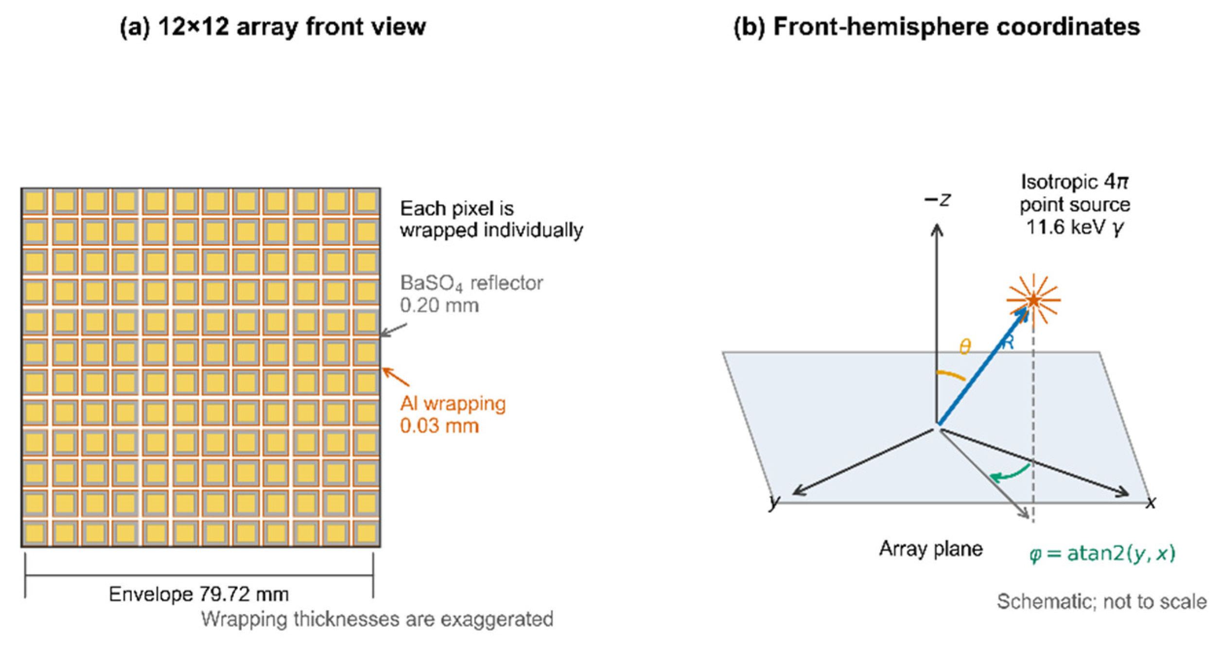
Figure 2.
Representative array-response heatmaps for four source positions. The score is the number of unique optical photons entering the optical adhesive layer.
Figure 2.
Representative array-response heatmaps for four source positions. The score is the number of unique optical photons entering the optical adhesive layer.
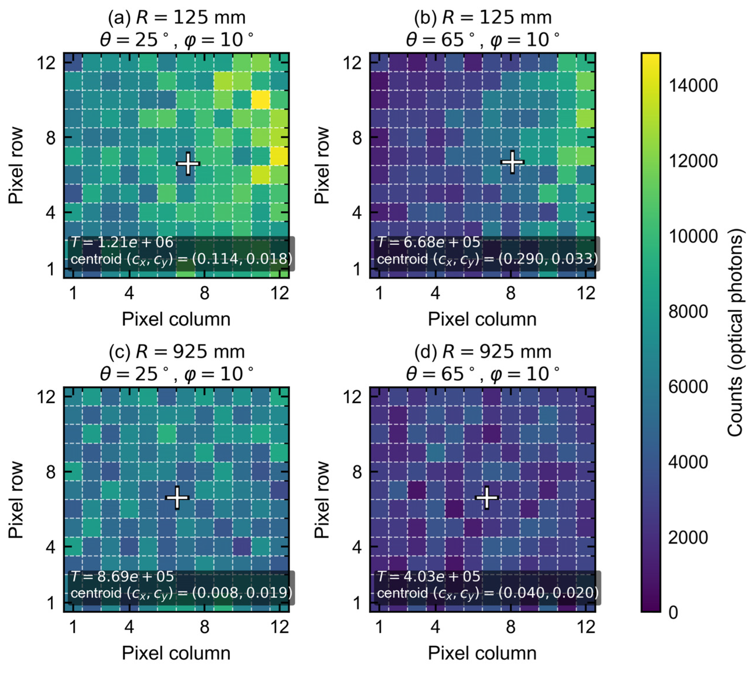
Figure 3.
Multi-distance scan grids and the training/validation/test partition: (a) staggered sampling in the R–θ plane; (b) grouped test positions in θ–φ–R space.
Figure 3.
Multi-distance scan grids and the training/validation/test partition: (a) staggered sampling in the R–θ plane; (b) grouped test positions in θ–φ–R space.
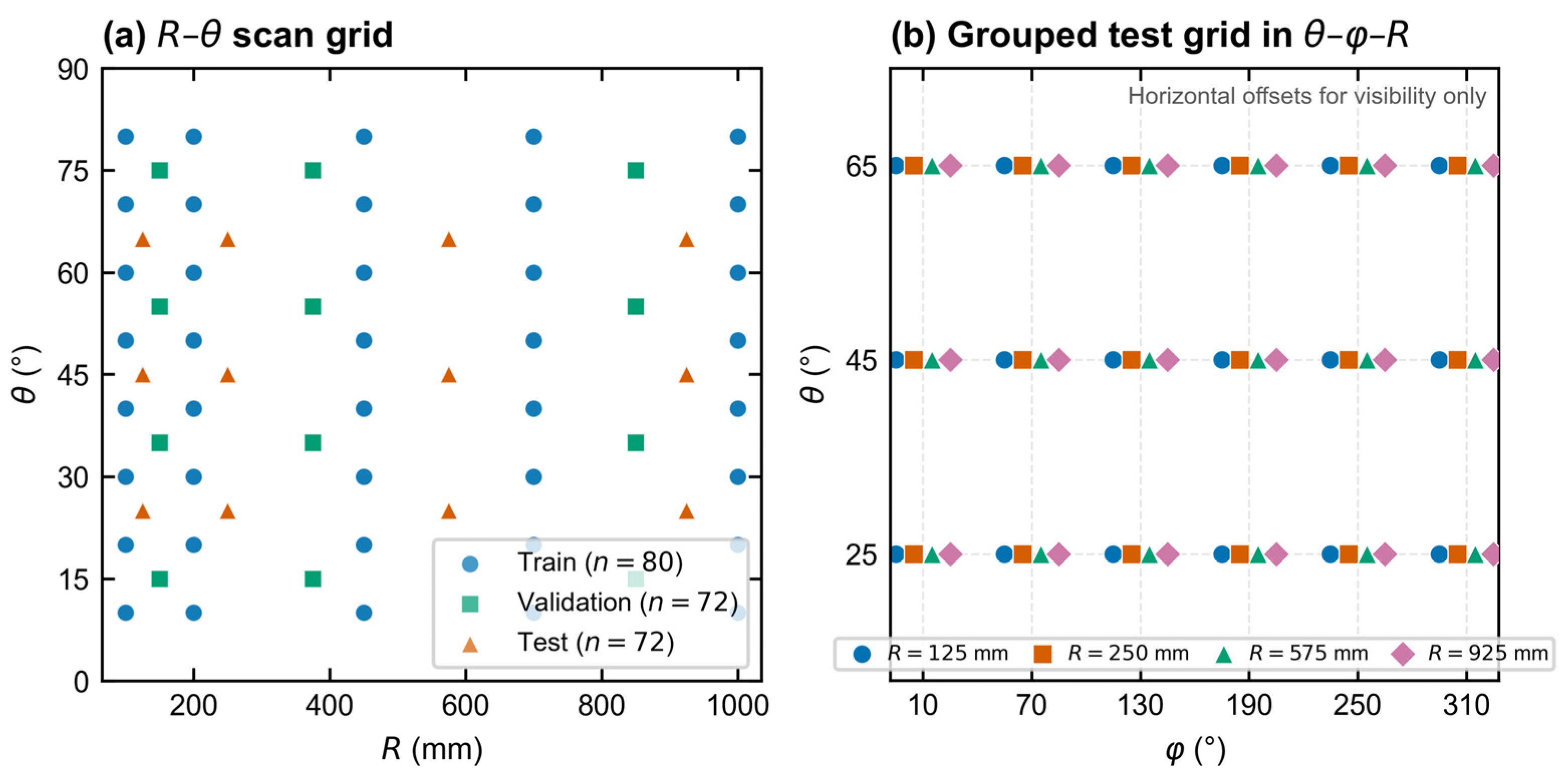
Figure 4.
Dual-branch CNN with spatial–global feature fusion. A convolutional encoder processes the normalized array response and coordinate channels, while an MLP encodes six global descriptors. The fused representation feeds separate direction and distance heads. The full model contains 41,876 trainable parameters.
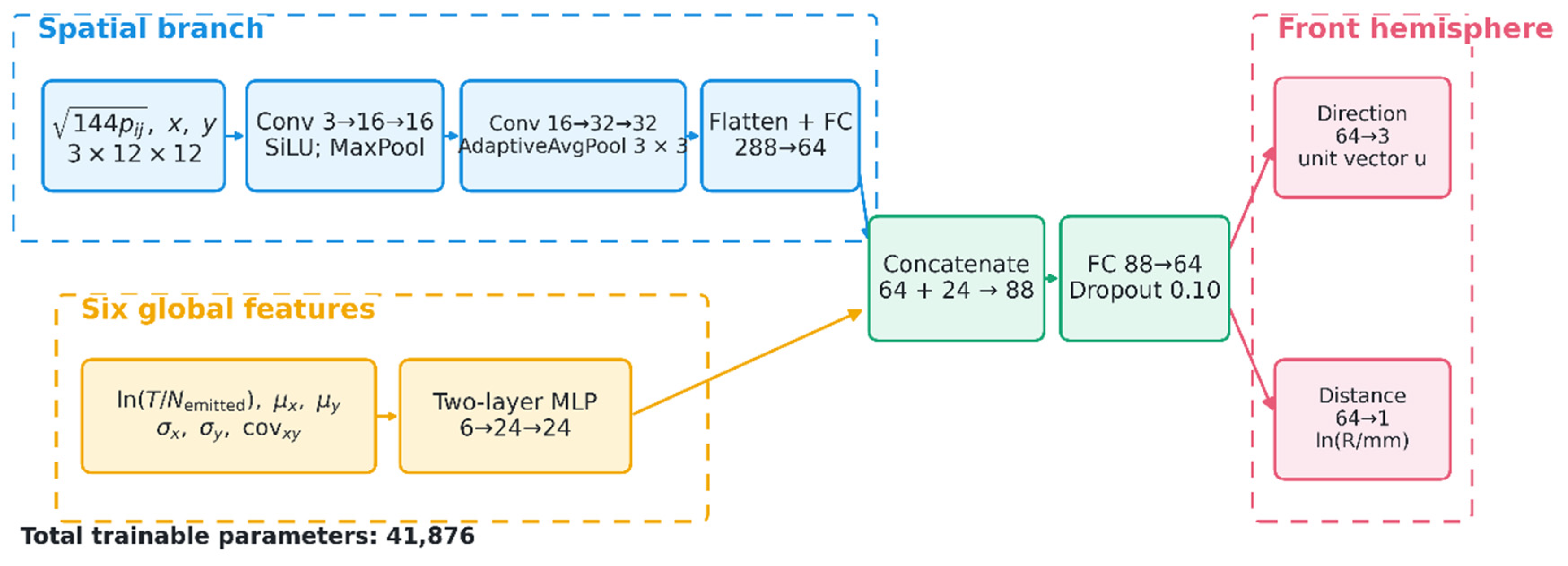
Figure 5.
Predictions and reference values on the 72-position held-out test set: (a) polar angle; (b) distance; and (c) distribution of circular azimuth error.
Figure 5.
Predictions and reference values on the 72-position held-out test set: (a) polar angle; (b) distance; and (c) distribution of circular azimuth error.
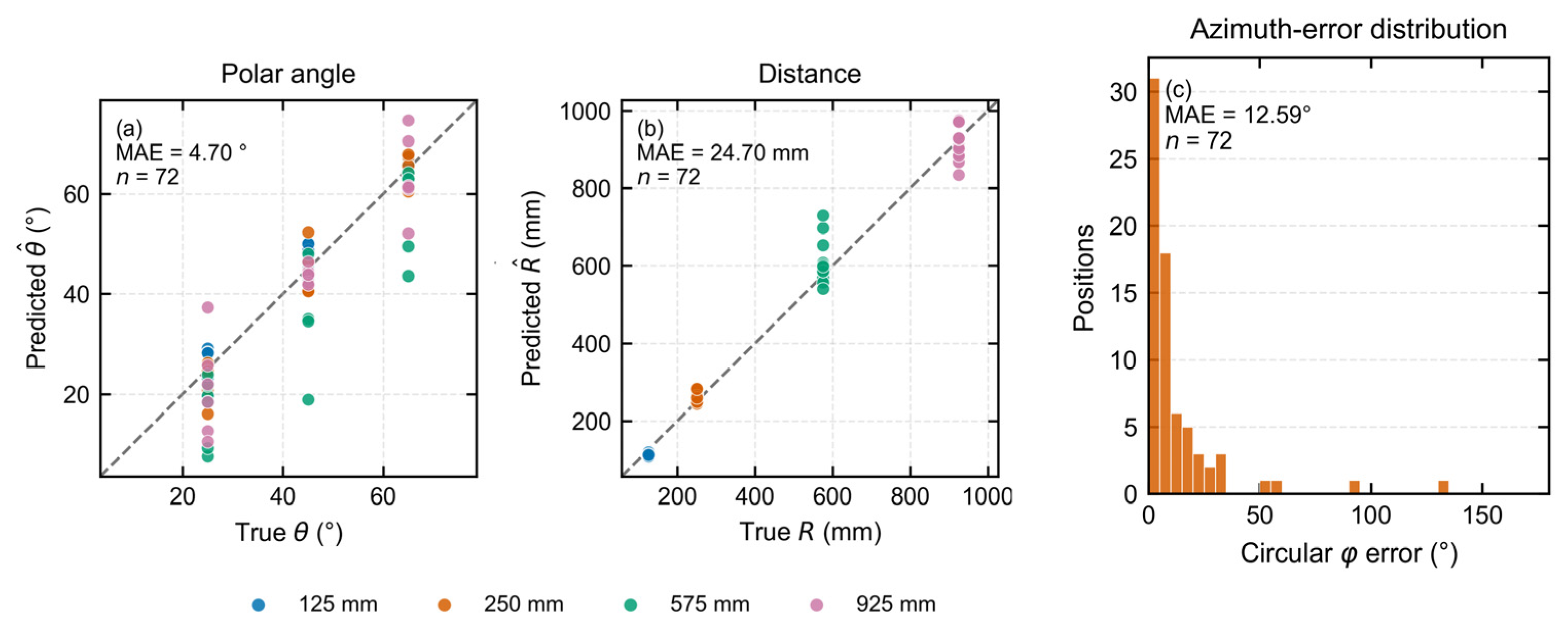
Figure 6.
Error variation across the held-out test set: (a) polar-angle MAE versus source distance; (b) circular azimuth MAE versus source distance; (c) three-dimensional directional MAE versus source distance; (d) distance MAPE versus source distance; and (e) circular azimuth MAE grouped by true polar angle.
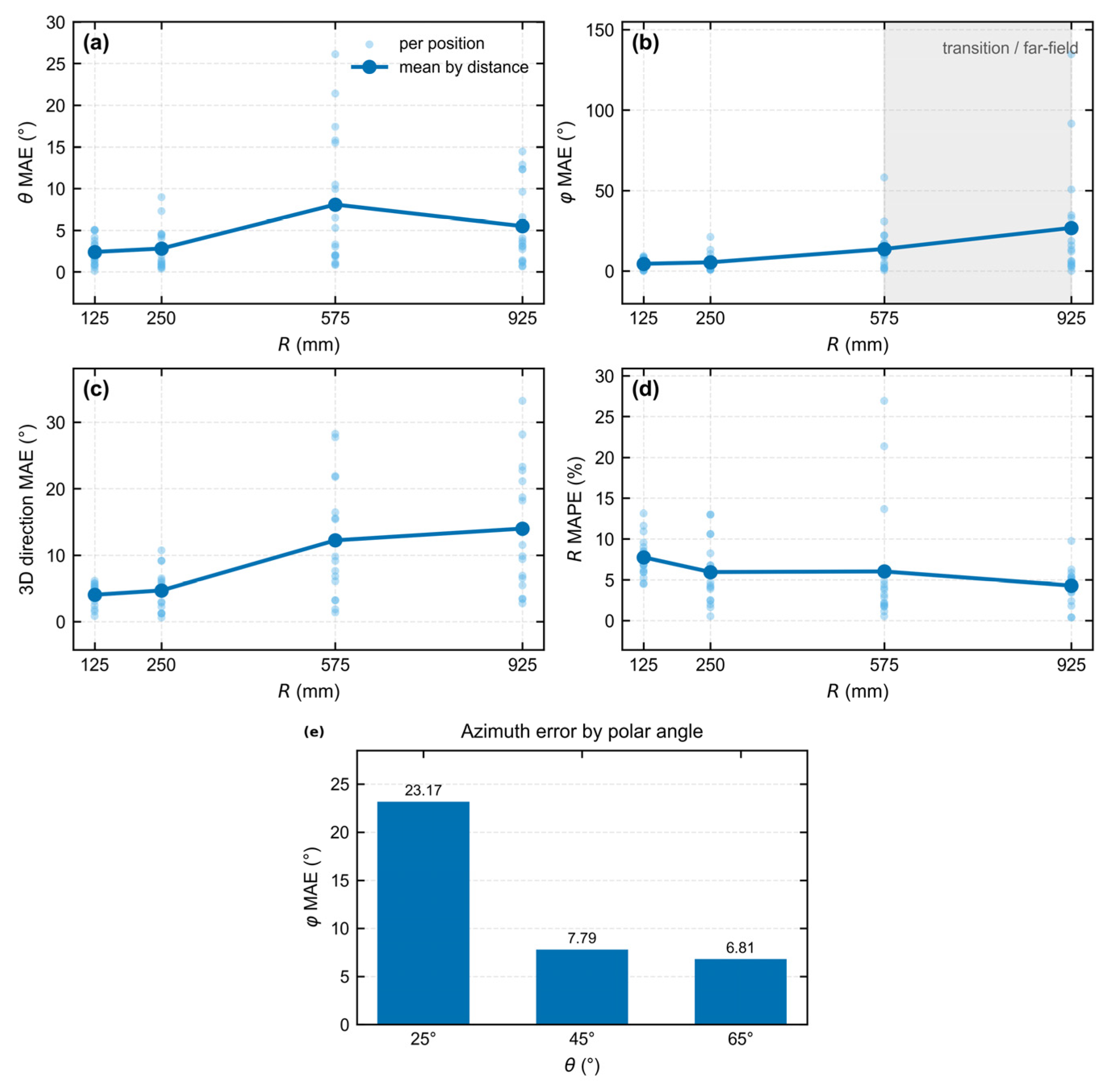
Figure 7.
Comparison of three-dimensional directional MAE and distance MAE on the 72-position test set. Neural-network bars show the mean across three seeds with between-seed SD; conventional baselines show one fixed run.
Figure 7.
Comparison of three-dimensional directional MAE and distance MAE on the 72-position test set. Neural-network bars show the mean across three seeds with between-seed SD; conventional baselines show one fixed run.
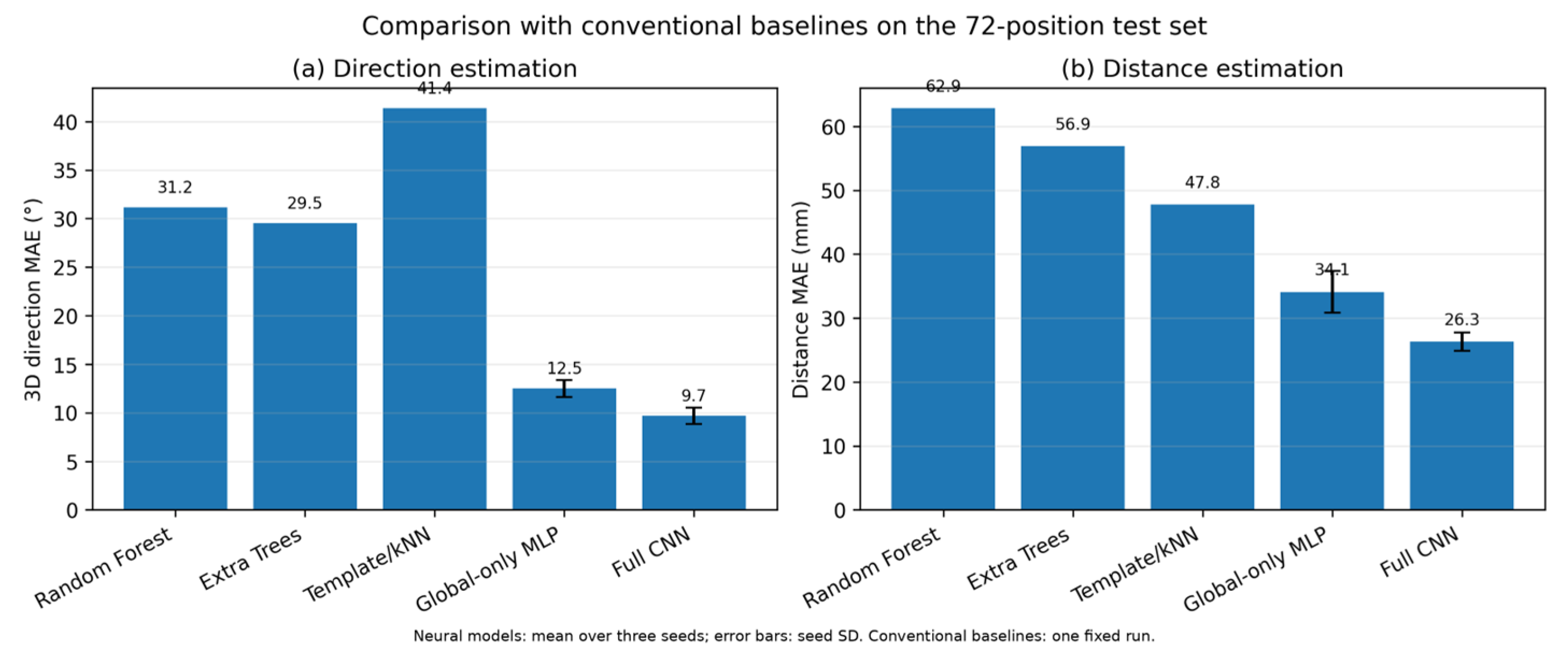
Figure 8.
Polar representation of three-dimensional directional error on the held-out test set across the sampled angle–distance grid.
Figure 8.
Polar representation of three-dimensional directional error on the held-out test set across the sampled angle–distance grid.
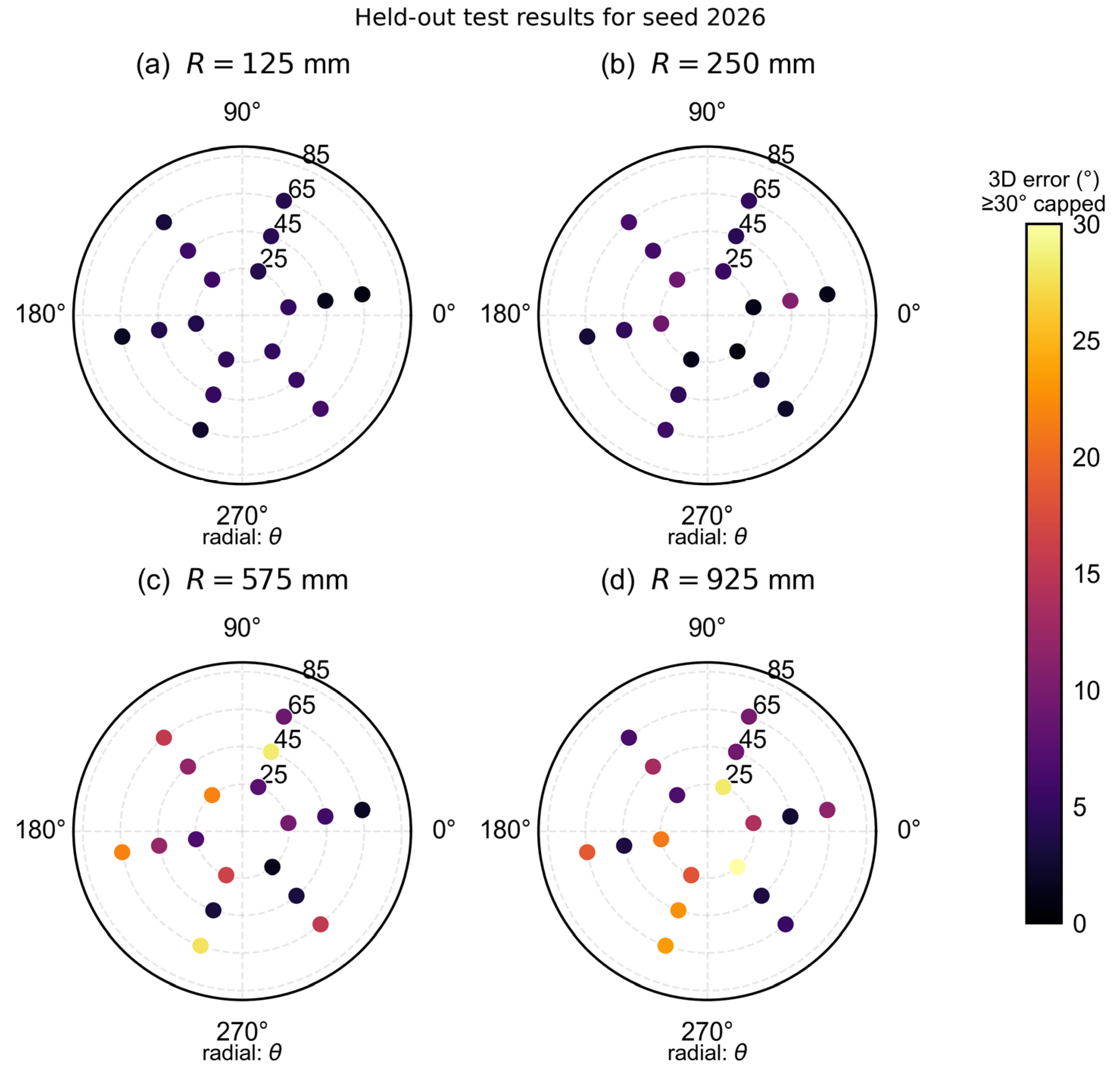
Figure 9.
Exposure-sensitivity analysis for six positions at R = 925 mm and θ = 25°: mean circular azimuth MAE versus exposure factor (1×, 2×, and 4×).
Figure 9.
Exposure-sensitivity analysis for six positions at R = 925 mm and θ = 25°: mean circular azimuth MAE versus exposure factor (1×, 2×, and 4×).
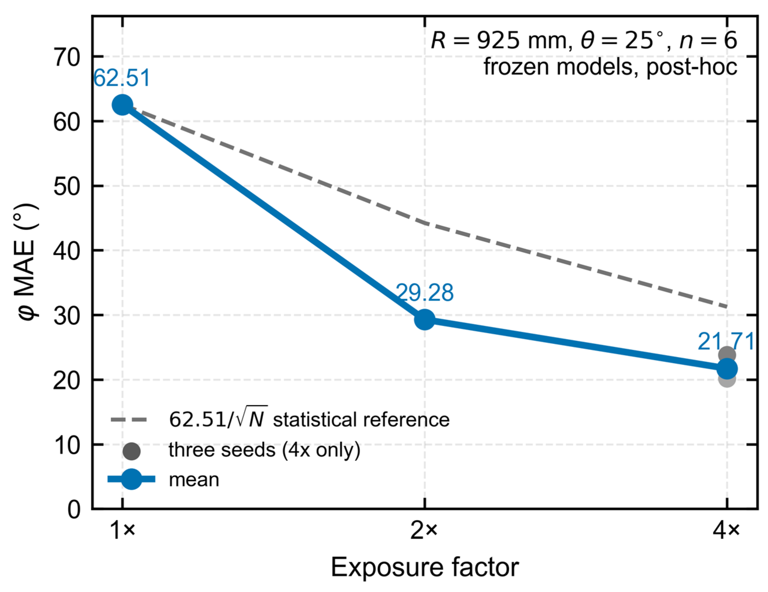
Figure 10.
Comparison of post-processing methods. Mean and worst circular azimuth errors are shown for the original CNN, four-rotation TTA, CNN–centroid fusion, and the centroid-only method.
Figure 10.
Comparison of post-processing methods. Mean and worst circular azimuth errors are shown for the original CNN, four-rotation TTA, CNN–centroid fusion, and the centroid-only method.
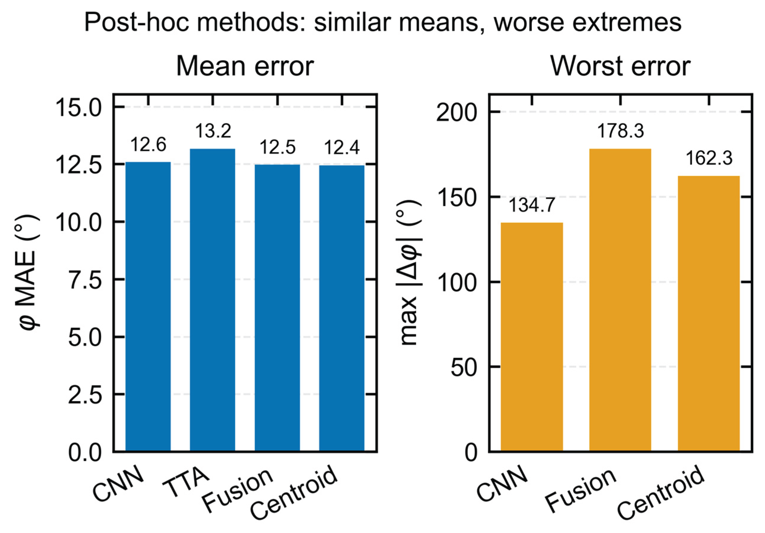
Table 1.
Main geometry and optical-modeling parameters of the 12 × 12 YSO array.
| Item | Parameter |
|---|---|
| Array | 12 × 12 (144 pixels) |
| Single crystal | 6.0 mm × 6.0 mm × 1.0 mm |
| YSO density | 4.45 g cm−3 |
| Lateral reflector | BaSO4, 0.20 mm |
| Lateral aluminum layer | 0.03 mm |
| Pixel pitch | 6.66 mm |
| Array envelope | Approximately 79.72 mm |
| Entrance-face reflector | ESR, 65 μm |
| Rear optical adhesive | 0.10 mm |
| Scintillation yield/decay time | 15,300 photons MeV⁻¹; 70 ns [16] |
Table 5.
Post-hoc ablation results on the 72-position test set (mean ± SD across three seeds).
| Model | Parameters | θ MAE (°) | φ MAE (°) | 3D MAE (°) | R MAE (mm) | R MAPE (%) |
|---|---|---|---|---|---|---|
| Full | 41,876 | 5.161 ± 0.422 | 13.558 ± 0.853 | 9.679 ± 0.838 | 26.333 ± 1.432 | 6.288 ± 0.262 |
| Shape-only | 39,572 | 8.413 ± 1.593 | 14.301 ± 1.849 | 12.560 ± 1.054 | 104.501 ± 17.122 | 20.392 ± 2.801 |
| Global-only | 2,628 | 6.917 ± 0.636 | 14.957 ± 0.447 | 12.506 ± 0.861 | 34.110 ± 3.285 | 7.758 ± 1.149 |
Table 6.
Comparison with conventional baselines on the 72-position test set.
| Model | θ MAE (°) | φ MAE (°) | 3D MAE (°) | R MAE (mm) | R MAPE (%) | 3D P95 (°) | R P95 (mm) |
|---|---|---|---|---|---|---|---|
| Random Forest | 12.459 | 45.720 | 31.152 | 62.865 | 19.411 | 80.610 | 167.177 |
| Extra Trees | 11.390 | 51.022 | 29.524 | 56.885 | 13.314 | 75.096 | 173.946 |
| Template/kNN | 18.731 | 65.048 | 41.378 | 47.785 | 15.609 | 90.134 | 125.000 |
| Global-only MLP | 6.917 ± 0.636 | 14.957 ± 0.447 | 12.506 ± 0.861 | 34.110 ± 3.285 | 7.758 ± 1.149 | 38.119 ± 4.324 | 91.331 ± 25.169 |
| Full CNN | 5.161 ± 0.422 | 13.558 ± 0.853 | 9.679 ± 0.838 | 26.333 ± 1.432 | 6.288 ± 0.262 | 25.200 ± 0.827 | 75.247 ± 7.986 |
Table 7.
Overall full-model results for three random initializations on the 72-position test set.
| Seed | θ MAE (°) | φ MAE (°) | 3D MAE (°) | R MAE (mm) | R MAPE (%) |
|---|---|---|---|---|---|
| 2026 | 4.70 | 12.59 | 8.75 | 24.70 | 6.00 |
| 2027 | 5.26 | 14.18 | 9.90 | 27.37 | 6.35 |
| 2028 | 5.52 | 13.90 | 10.38 | 26.94 | 6.51 |
| Mean ± seed SD | 5.16 ± 0.42 | 13.56 ± 0.85 | 9.68 ± 0.84 | 26.33 ± 1.43 | 6.29 ± 0.26 |
Disclaimer/Publisher’s Note: The statements, opinions and data contained in all publications are solely those of the individual author(s) and contributor(s) and not of MDPI and/or the editor(s). MDPI and/or the editor(s) disclaim responsibility for any injury to people or property resulting from any ideas, methods, instructions or products referred to in the content. |
© 2026 by the authors. Licensee MDPI, Basel, Switzerland. This article is an open access article distributed under the terms and conditions of the Creative Commons Attribution (CC BY) license.
Copyright: This open access article is published under a Creative Commons CC BY 4.0 license, which permit the free download, distribution, and reuse, provided that the author and preprint are cited in any reuse.