
Submitted:
28 September 2026
Posted:
29 September 2026
You are already at the latest version
Abstract
One way to give robots a sense of touch is a magnetic tactile sensor: a magnet sits inside a soft skin above a Hall-effect sensor, and pressing the skin moves the magnet and changes the field the sensor reads. Most studies change the magnet, sensor, and skin together, so the effect of the skin is hard to isolate. We asked how the internal structure and material of the skin change the sensor's sensitivity, repeatability, and hysteresis with everything else fixed. We hypothesized that skins that deform more under load would produce larger magnetic signals, so that cast silicone and open lattices would be the most sensitive and lattices enclosed by a solid wall would be the least. We simulated solid, honeycomb, and gyroid blocks in ANSYS, then built five skins (cast silicone and four 3D-printed TPU lattices) and loaded each from 0 to 80 g and back three times above an MLX90393 sensor. Silicone was the most sensitive skin (0.135 µT/g), followed by a 10% honeycomb (0.084 µT/g) and a 10% gyroid (0.063 µT/g), even though simulation predicted the gyroid would deform 22 times more than the honeycomb. An outer wall almost erased the response of a 5% gyroid, while a walled 5% hexagonal lattice gave the most repeatable readings. Skin design changed sensitivity more than tenfold, and the most sensitive skin was also the least repeatable, so the best skin depends on what the sensor is for.
Keywords:
magnetic tactile sensing
; Hall-effect sensor
; TPU lattice structure
; silicone skin
; load-unload hysteresis
; sensor
; Hall sensor
1. Introduction
A camera can show a robot where an object is, but once the gripper closes, the camera mostly sees the back of the robot’s own fingers. What happens at the contact itself, such as how hard the grip is, whether the object is starting to slip, and where exactly it is touching, has to be felt. Tactile sensing has helped robots predict whether a grasp will succeed [1], control a remote gripper with force feedback [2], track an object as it moves in the hand [3], and catch mistakes while cutting vegetables [4].
Engineers have built touch sensors around several physical effects. Piezoresistive sensors use materials whose electrical resistance changes when they are squeezed, which makes them easy to build into flexible skins, but their output can drift depending on how they were loaded before [5]. Optical sensors such as GelSight place a camera behind a soft gel and read the shape of whatever presses into it, which gives very detailed contact images but needs space for the camera and carefully controlled lighting [6,7,8]. Magnetic sensors work differently. A magnet is embedded in a soft skin, a Hall-effect sensor underneath measures the magnetic field, and pressing on the skin moves the magnet and changes that field [9,10,11]. The electronics never touch the object, and the parts are cheap and easy to replace.
A Hall-effect sensor does not measure force directly. It measures magnetic flux density along three axes, usually written Bx, By, and Bz. When the skin is pressed, the magnet moves down, slides sideways, or tilts, and each kind of motion changes the three readings in a different way. A calibration model then converts the change in field back into force or contact location [12,13,14]. This conversion is not simple, because the field from a small magnet falls off steeply with distance, so the same push can produce very different signals depending on where the magnet starts [12]. Researchers have handled this with neural networks [9], models that correct for differences between individual magnets [14], and automated setups that press the sensor at known forces and positions to collect calibration data [15,16,17].
Most of this work focuses on the magnet, the electronics, or the calibration model. The soft skin between the magnet and the outside world gets less attention, even though it decides how far the magnet moves for each gram of applied mass. A softer skin lets the magnet travel farther and gives a bigger signal, but it reaches its limit at lower forces and tends to creep over time. A stiffer skin handles larger forces but produces a weaker signal [12,15]. In most published sensors, though, the skin changes together with the magnet layout and the sensor arrangement [12,13,15], so it is hard to tell how much of a sensor’s performance comes from the skin alone.
3D printing offers a cheap way to tune the skin without changing its material. Thermoplastic polyurethane (TPU) is a flexible printing filament, and slicing software can fill a printed part with different internal patterns at different densities, called infill. A honeycomb lattice is built from hexagonal cells. A gyroid lattice is a single wavy surface that repeats in all three directions, with no flat walls or sharp corners. Changing the pattern or the infill percentage changes how stiff the part is, even though every part is made of the same plastic. The usual alternative, casting silicone rubber in a mold, gives a softer and more uniform skin but is harder to vary in a controlled way.
In this study, we held the magnet, the MLX90393 three-axis Hall-effect sensor, and the 10 mm gap between them fixed and changed only the skin. We first used finite-element simulation to compare how solid, honeycomb, and gyroid TPU blocks deform under light loads. We then tested five real skins: cast silicone, a 10% gyroid and a 10% honeycomb with open sides, and a 5% gyroid and a 5% hexagonal lattice, each enclosed by a thin solid wall. We hypothesized that skins that deform more under load would move the magnet farther and give higher sensitivity, so that silicone and the open lattices would be the most sensitive and the walled lattices the least, and that the simulated deformation of each lattice would predict its measured ranking. Silicone was the most sensitive skin and the walled 5% gyroid barely responded, but the honeycomb beat the gyroid even though the simulation predicted the opposite. The most sensitive skin was also the least repeatable. These results indicate that the internal structure of a printed skin can change a magnetic tactile sensor’s sensitivity by more than ten times with no change in hardware, and that simulated peak deformation is a poor guide for choosing between lattices.
2. Materials and Methods
2.1. Specimen Design and Finite-Element Simulation
Three TPU blocks measuring 25 × 25 × 22 mm were modeled in CAD, each with a central cylindrical pocket (8 mm diameter, 3 mm deep) at mid-height to hold the magnet: a solid reference block, a honeycomb lattice block, and a gyroid lattice block (Figure 1). All bodies were assigned isotropic, linear elastic TPU properties matched to the printing filament. Static structural analyses were run in ANSYS Mechanical 2026 R1 Student (Ansys Inc.) using a tetrahedral mesh with a default element size of about 2.2 mm (15,000 to 17,000 elements per body). The bottom face of each block was fixed, and a uniform normal force of 0.2, 0.4, 0.6, or 0.8 N was applied to the top face, matching the 20 to 80 g masses used in the experiments. Total deformation, equivalent elastic strain, equivalent (von Mises) stress, and safety factor relative to the 8.6 MPa tensile yield strength were recorded for each case.
2.2. Skin Fabrication
Five skin configurations were fabricated (Figure 1): a cast silicone skin, a 10% infill honeycomb lattice, a 10% infill triply-periodic gyroid lattice, a 5% triply-periodic infill gyroid lattice enclosed by a thin solid wall, and a 5% infill hexagonal lattice enclosed by the same type of wall. The silicone skin was cast from liquid silicone rubber Siloczest in a 3D-printed mold. The four lattice skins were 3D printed from TPU filament Wol3d on a Flashforge Adventure 5M printer. A neodymium (NdFeB) disc magnet, 8 mm in diameter and 3 mm thick wukong, was embedded at mid-height in each skin so that the magnet sat in the same position in every sample.
2.3. Sensing Setup and Loading Protocol
Magnetic field was measured with an MLX90393 three-axis Hall-effect magnetometer (SmartElex) connected to an ESP32 DevKit microcontroller board (Espressif Systems) over an I2C interface (Figure 2). The sensor was held in a rigid 3D-printed mount that fixed the magnet-to-sensor distance at 10 mm for every skin. This distance was chosen in preliminary trials because it gave the most reproducible readings. Masses were placed on the top surface of each skin in 20 g steps from 0 to 80 g and then removed in the same steps back to 0 g, giving nine load stages. Each stage was held for about 10 s before the next change. The ΔX, ΔY, and ΔZ field components were recorded continuously, and the full cycle was repeated three times for each configuration.
2.4. Data Processing and Statistical Analysis
Only the vertical field component was analyzed. For each load stage, the mean response was calculated from readings taken during the roughly 10 s plateau and expressed relative to the initial unloaded baseline (Equation 1):
where Zi is the mean field at load stage i and Z0 is the mean field at the initial 0 g stage. Sensitivity S (µT/g) was calculated as the slope of a least-squares line fitted to ΔZ against applied mass m on the loading leg (Equation 2):
ΔZi = Zi − Z0
Hysteresis H was calculated as the mean absolute difference between the loading (L) and unloading (U) responses at 20, 40, and 60 g (Equation 3):
Residual zero-load offset P was calculated as the difference between the final and initial 0 g readings (Equation 4):
Intra-run noise was taken as the scatter of ΔZ within the load plateaus of a single run, and inter-run repeatability as the spread between the three runs at matching load stages. Results are reported as the mean ± standard deviation (SD) of the three runs. Peak responses at 80 g were compared across configurations with a one-way ANOVA followed by Tukey’s honestly significant difference test, with significance set at p < 0.05.
3. Results
To isolate the effect of the skin, we kept the magnet, sensor, and electronics identical in every test and varied only the internal structure and material of the skin. We began with simulations of three TPU block designs, then fabricated five skins (Figure 1) and tested each one above the same MLX90393 sensor at a fixed 10 mm gap (Figure 2).
3.1. Simulation Predicted Large Differences in Deformation Between Lattice Types
Before printing anything, we wanted to know how much each internal geometry would let the magnet pocket move under light loads. We modeled solid, honeycomb, and gyroid blocks (25 × 25 × 22 mm) in ANSYS Mechanical, fixed the bottom face, and pressed on the top face with forces of 0.2 to 0.8 N, which match the 20 to 80 g masses used later in the experiments. Deformation increased in proportion to force for all three geometries, and the differences between them were huge (Table 1). At 0.8 N, the solid block deformed by 5.17 × 10⁻⁴ mm, the honeycomb by 0.0222 mm (about 43 times more), and the gyroid by 0.485 mm (about 940 times the solid and 22 times the honeycomb). The contour plots show where this movement happened (Figure 3). The honeycomb compressed fairly evenly from top to bottom, while the largest deformation in the gyroid sat on a thin, unsupported edge of the lattice at the top of the block rather than around the center, where the magnet sits. Maximum stress followed the same order, reaching 0.0028 MPa in the solid, 0.056 MPa in the honeycomb, and 0.397 MPa in the gyroid at 0.8 N (Figure 3). All of these values were far below the 8.6 MPa yield strength of TPU, and the safety factor stayed above 10 in every case (Table 1), so none of the designs was expected to deform permanently under the test loads.
3.2. Each Load Step Produced a Clear, Stable Plateau in the Magnetic Signal
We then placed each skin over the sensor and loaded it with masses from 0 to 80 g in 20 g steps and back down to 0 g, holding each stage for about 10 s and repeating the full cycle three times. Raw traces from the 10% gyroid, cast silicone, and 10% honeycomb skins showed a flat plateau at every stage, with a sharp jump each time a mass was added or removed (Figure 4). At 80 g, the silicone trace rose the most, the gyroid the least, and the honeycomb fell in between. The gyroid trace also finished roughly 2 µT above where it started, a first sign that some skins did not fully spring back. Signal noise within a plateau was similar for all five skins, between 0.24 and 0.29 µT (Table 2), which was expected because every skin used the same sensor and electronics.
3.3. Silicone Gave the Largest Response, and the Honeycomb Outperformed the Gyroid
Averaging the three runs gave a hysteresis loop for each skin, in which the signal climbed as mass was added and fell as it was removed (Figure 5). Peak response at 80 g was 10.88 ± 1.36 µT for silicone, 6.90 ± 0.38 µT for the 10% honeycomb, 5.04 ± 0.17 µT for the 10% gyroid, and 4.05 ± 0.16 µT for the walled 5% hexagonal lattice (mean ± SD, n = 3; Table 2). Peak response differed across skins (one-way ANOVA, F(4, 10) = 117.4, p < 0.001). Tukey’s post hoc test showed that silicone exceeded the honeycomb (p < 0.001) and that the honeycomb exceeded the 10% gyroid (p = 0.048), while the 10% gyroid and the 5% hexagonal lattice were not significantly different (p = 0.44). The response rose roughly linearly with mass on both the loading and unloading legs (Figure 6), so we summarized each skin by the slope of its loading leg. Sensitivity was 0.135 µT/g for silicone, 0.084 µT/g for the honeycomb, 0.063 µT/g for the 10% gyroid, 0.050 µT/g for the 5% hexagonal lattice, and 0.010 µT/g in magnitude for the walled 5% gyroid (Figure 6). The simulation had ranked the gyroid far ahead of the honeycomb, but in the real sensor the honeycomb was about 1.3 times as sensitive.
3.4. A Solid Outer Wall Drastically Reduced the Response of the 5% Gyroid
The walled 5% gyroid behaved differently from every other skin. Its signal stayed small in all three runs and moved slightly in the wrong direction, reaching −0.89 ± 0.55 µT at 80 g with a loading slope of −0.010 µT/g (Figure 5). That peak was comparable to the 0.54 µT spread between its own repeat runs (Table 2). The 5% hexagonal lattice had the same kind of wall and the same infill, yet it still produced 4.05 µT at 80 g. This suggests that confinement interacts strongly with the internal lattice architecture, although the present experiment does not isolate wall thickness as an independent variable.
3.5. Higher Sensitivity Came with Poorer Repeatability
A large signal is only useful if the sensor gives the same reading for the same load, so we also compared how consistent each skin was (Figure 6). Silicone had the largest spread between repeat runs, 0.92 µT, followed by the walled 5% gyroid at 0.54 µT and the honeycomb at 0.31 µT. The 10% gyroid (0.10 µT) and the 5% hexagonal lattice (0.06 µT) were the most repeatable (Figure 6). Hysteresis, the average gap between the loading and unloading curves, was highest for the 10% gyroid at 1.15 µT and lowest for the honeycomb (0.59 µT) and silicone (0.61 µT), with the 5% hexagonal lattice in between at 0.84 µT (Figure 6). After the last mass was removed, silicone and the honeycomb returned almost exactly to their starting readings, with residual zero-load offset of 0.02 ± 0.35 µT and 0.05 ± 0.38 µT. The 10% gyroid and the 5% hexagonal lattice did not, ending 1.02 ± 1.06 µT and 1.10 ± 0.04 µT above their starting values (Figure 6).
4. Discussion
We set out to find how much the behavior of a magnetic tactile sensor depends on its skin when the magnet, sensor, and electronics stay the same. The skin turned out to matter a great deal. Sensitivity ranged from 0.135 µT/g for cast silicone down to essentially zero for the walled 5% gyroid, and that difference came entirely from the material and internal structure of a 25 mm block. Our hypothesis was partly supported. Silicone, the softest skin, gave the largest signal, and the walled gyroid gave the smallest, as we expected. The prediction that simulated deformation would rank the lattices correctly did not hold, because the honeycomb beat the gyroid in the real sensor even though the simulation predicted the gyroid would deform 22 times more.
We hypothesized this mismatch comes from the fact that simulations could not fully account for the internal structure infills. ANSYS gives the largest displacement anywhere in the part, and in the gyroid that maximum sat on a thin edge of the lattice at the top of the block (Figure 3). An edge bending near the surface says little about how far the magnet at the center moves. The honeycomb deformed more evenly through its height, so more of its compression probably reached the magnet pocket. Maximum global deformation is not necessarily the relevant mechanical variable for a magnetic tactile sensor. The simulation also treated TPU as a uniform, perfectly elastic solid, while real printed parts have layer lines, small gaps between printed strands, and infill generated by the slicer that does not exactly match the CAD lattice. Silicone was not simulated at all. A more useful simulation would track the displacement of the magnet pocket itself, since that is what the Hall-effect sensor actually responds to.
The lead of silicone in sensitivity makes sense because cast silicone rubber is much softer than printed TPU and fills the whole block, so the load spreads evenly and pushes the magnet straight down. That same softness probably explains why silicone was the least repeatable skin. Soft rubber creeps under load, so the magnet may settle at a slightly different depth each time, and because the magnetic field changes steeply with distance, small differences in magnet position show up as large differences in the reading. Placing the masses by hand may also have loaded the soft silicone slightly off center from run to run. The spread between silicone runs was about 8% of its peak signal, while the spread for the 5% hexagonal lattice was under 2% of its peak.
The walled 5% gyroid was the most surprising result. With only 5% infill, the gyroid inside is very sparse, so the solid outer wall probably carried nearly all of the load straight down to the base while the lattice around the magnet barely moved. The 5% hexagonal lattice sat inside the same kind of wall and still produced a clear signal. One possibility is that its cell walls tie the top surface to the region around the magnet more directly than the sparse gyroid does, so the magnet moves along with the top surface. We did not vary wall thickness or image the lattices while they were loaded, so this explanation still needs to be tested. The result does show that adding a wall can make a lattice skin almost useless as a sensor, depending on the lattice architecture.
Residual zero-load offset matters for any sensor that has to read zero when nothing is touching it. The simulations predicted stresses far below the yield strength of TPU, so the offsets we saw in the 10% gyroid and the 5% hexagonal lattice are unlikely to come from the plastic bending permanently. A more likely cause is that TPU recovers slowly after being unloaded, and a 10 s hold at 0 g was not long enough for these lattices to spring fully back. The magnet may also shift slightly inside its pocket. For the 10% gyroid, the offset averaged 1.02 µT, about 20% of its peak signal, and varied widely between runs, so it could not simply be subtracted out. The 5% hexagonal lattice ended 1.10 µT high, but almost identically each time (± 0.04 µT), which suggests its offset could be removed with a fixed correction or a few break-in cycles before use.
These trade-offs point to different uses for different skins. Silicone would suit a sensor that needs to detect light touches, where a large signal matters more than exact repeatability. The 5% hexagonal lattice would suit a sensor that must give the same reading for the same force every time, such as a gripper that holds objects at a set force. The honeycomb offered the best balance in our tests, with the second-highest sensitivity, low hysteresis, and almost no residual zero-load offset. Because all four lattices were printed from one material, a designer could move between these behaviors by changing slicer settings, without touching the electronics. We tested only one sensor layout at loads up to 80 g, however, so these rankings may change for other magnets, gaps, or force ranges.
Several limits of this study affect how far the results can be pushed. Each configuration was tested in only three runs, which is enough to separate the large differences but not to pin down the smaller ones, and the large spread for silicone makes its exact sensitivity uncertain. Testing several independently printed copies of each design would show how much of the variation comes from the design and how much from differences between prints. We analyzed only the vertical field component and applied only normal loads, while real contacts also push sideways. The masses were placed by hand, and the 10 s hold at each stage was too short to measure slow creep. The simulations and experiments also did not use identical geometries or materials, which limits how directly they can be compared.
Future tests could link simulation and measurement more closely by simulating the displacement of the magnet pocket and printing lattices that match the simulated geometry exactly. Sweeping infill percentage and wall thickness in smaller steps, adding shear loads, using all three field components, and running hundreds of load cycles would show whether the residual zero-load offset keeps growing or levels off. An automated loading system, such as a 3D printer fitted with a probe [17], would remove the variation from hand-placed masses and make these larger test sets practical.
By changing only the skin of a magnetic tactile sensor, we changed its sensitivity by more than ten times and found a clear trade-off between sensitivity and repeatability. Cast silicone gave the strongest signal, the honeycomb gave the best balance, and a walled 5% hexagonal lattice gave the most consistent readings, while a walled 5% gyroid produced almost no signal. Simulated peak deformation did not predict which lattice would perform best. For anyone building low-cost tactile sensors, the skin deserves as much design attention as the magnet and the electronics, and 3D-printed lattices offer an easy way to tune it.
Author Contributions
Conceptualization, A.J.; Methodology, A.J. and N.P.; Validation, N.P.; Formal analysis, A.J. and N.P.; Investigation, A.J. and N.P.; Resources, R.J.; Writing - original draft, A.J. and N.P.; Writing - review and editing, A.J., N.P. and R.J.; Visualization, A.J.; Supervision, N.P.; Project administration, R.J.; All authors have read and agreed to the published version of the manuscript.
Funding
This research received no external funding.
Institutional Review Board Statement
Not applicable.
Informed Consent Statement
Not applicable.
Data Availability Statement
To be uploaded.
Acknowledgments
During the preparation of this manuscript, the author(s) used Claude AI to review the manuscript; and to change from the original formatting to preprint template. The authors have reviewed and edited the output and take full responsibility for the content of this publication.
Conflicts of Interest
The authors declare no conflicts of interest.
References
- Calandra, R.; et al. The Feeling of Success: Does Touch Sensing Help Predict Grasp Outcomes? In Proceedings of the 1st Annual Conference on Robot Learning, 2017; Volume 78, pp. 314-323. https://proceedings.mlr.press/v78/calandra17a.html.
- Lippi, M.; et al. Low-Cost Teleoperation with Haptic Feedback through Vision-Based Tactile Sensors for Rigid and Soft Object Manipulation. In Proceedings of the 2024 33rd IEEE International Conference on Robot and Human Interactive Communication (RO-MAN), 2024; pp. 1963-1969. [CrossRef]
- Sodhi, P.; et al. PatchGraph: In-Hand Tactile Tracking with Learned Surface Normals. In Proceedings of the 2022 International Conference on Robotics and Automation (ICRA), 2022; pp. 2164-2170. [CrossRef]
- Yamaguchi, A.; Atkeson, C.G. Combining Finger Vision and Optical Tactile Sensing: Reducing and Handling Errors While Cutting Vegetables. In Proceedings of the 2016 IEEE-RAS 16th International Conference on Humanoid Robots (Humanoids), 2016; pp. 1045-1051. [CrossRef]
- Stassi, S.; et al. Flexible Tactile Sensing Based on Piezoresistive Composites: A Review. Sensors 2014, 14, 5296-5332. [CrossRef]
- Yuan, W.; et al. GelSight: High-Resolution Robot Tactile Sensors for Estimating Geometry and Force. Sensors 2017, 17, 2762. [CrossRef]
- Johnson, M.K.; Adelson, E.H. Retrographic Sensing for the Measurement of Surface Texture and Shape. In Proceedings of the 2009 IEEE Conference on Computer Vision and Pattern Recognition, 2009; pp. 1070-1077. [CrossRef]
- Johnson, M.K.; et al. Microgeometry Capture Using an Elastomeric Sensor. ACM Trans. Graph. 2011, 30. [CrossRef]
- Hellebrekers, T.; et al. Soft Magnetic Tactile Skin for Continuous Force and Location Estimation Using Neural Networks. IEEE Robot. Autom. Lett. 2020, 5, 3892-3898. [CrossRef]
- Tomo, T.P.; et al. Design and Characterization of a Three-Axis Hall Effect-Based Soft Skin Sensor. Sensors 2016, 16, 491. [CrossRef]
- Bhirangi, R.; et al. ReSkin: Versatile, Replaceable, Lasting Tactile Skins. In Proceedings of the 5th Conference on Robot Learning, 2021. https://openreview.net/forum?id=87_OJU4sw3V.
- Wang, H.; et al. Design Methodology for Magnetic Field-Based Soft Tri-Axis Tactile Sensors. Sensors 2016, 16, 1356. [CrossRef]
- Mohammadi, A.; et al. Magnetic-Based Soft Tactile Sensors with Deformable Continuous Force Transfer Medium for Resolving Contact Locations in Robotic Grasping and Manipulation. Sensors 2019, 19, 4925. [CrossRef]
- Yang, X.; et al. Robust Estimation of Contact Force and Location for Magnetic-Field-Based Soft Tactile Sensor Considering Magnetic Source Inconsistency. Sensors 2021, 21, 5388. [CrossRef]
- Rehan, M.; et al. A Soft Multi-Axis High Force Range Magnetic Tactile Sensor for Force Feedback in Robotic Surgical Systems. Sensors 2022, 22, 3500. [CrossRef]
- Van den Stockt, L.; et al. Automatic Calibration for an Open-Source Magnetic Tactile Sensor. arXiv 2024. https://arxiv.org/abs/2405.18582.
- Kota, R.; et al. 3D Cal: An Open-Source Software Library for Calibrating Tactile Sensors. arXiv 2025. https://arxiv.org/abs/2511.03078.
Figure 1.
CAD models and fabricated skin samples. CAD models were renderings of 25 × 25 × 22 mm TPU blocks, each with a central cylindrical magnet pocket (8 mm diameter, 3 mm deep) at mid-height. Lattice skins were 3D printed in TPU. The silicone skin was cast in a 3D-printed mold. Each skin holds an 8 × 3 mm NdFeB magnet at mid-height. a) CAD model of solid skin (b) CAD model of the honeycomb lattice c) CAD model of the gyroid d) cast of the silicone skin e) 3D printed 10% infill honeycomb lattice f) 3D printed 10% infill triply-periodic gyroid lattice without a wall g) 3D printed 5% infill hex lattice with thin outer wall h) 3D printed 5% infill triply-periodic gyroid lattice with thin outer wall.
Figure 1.
CAD models and fabricated skin samples. CAD models were renderings of 25 × 25 × 22 mm TPU blocks, each with a central cylindrical magnet pocket (8 mm diameter, 3 mm deep) at mid-height. Lattice skins were 3D printed in TPU. The silicone skin was cast in a 3D-printed mold. Each skin holds an 8 × 3 mm NdFeB magnet at mid-height. a) CAD model of solid skin (b) CAD model of the honeycomb lattice c) CAD model of the gyroid d) cast of the silicone skin e) 3D printed 10% infill honeycomb lattice f) 3D printed 10% infill triply-periodic gyroid lattice without a wall g) 3D printed 5% infill hex lattice with thin outer wall h) 3D printed 5% infill triply-periodic gyroid lattice with thin outer wall.
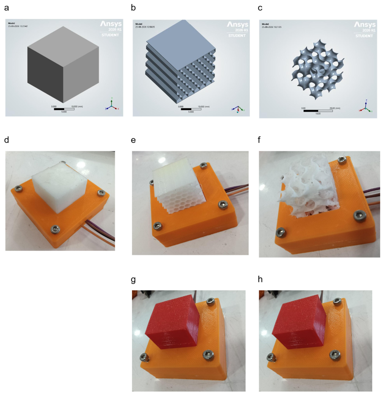
Figure 2.
Magnetic sensing setup. (a) 3D-printed mount holding the MLX90393 three-axis Hall-effect sensor at a fixed 10 mm gap below the magnet in each skin. (b) Circuit schematic connecting the MLX90393 to an ESP32 DevKit over I2C.
Figure 2.
Magnetic sensing setup. (a) 3D-printed mount holding the MLX90393 three-axis Hall-effect sensor at a fixed 10 mm gap below the magnet in each skin. (b) Circuit schematic connecting the MLX90393 to an ESP32 DevKit over I2C.
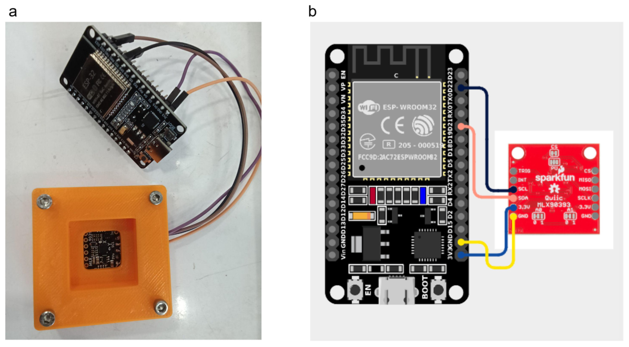
Figure 3.
Deformation in the gyroid was concentrated at thin lattice edges. Simulated stress was highest in the gyroid lattice. ANSYS total deformation contour plots at 0.8 N for the (a) solid, (b) honeycomb, and (c) gyroid blocks. Red marks maximum and blue marks minimum deformation. Color scales differ between panels (maximum 0.00052, 0.022, and 0.485 mm). ANSYS equivalent (von Mises) stress contour plots at 0.8 N for the (d) solid, (e) honeycomb, and (f) gyroid blocks. Color scales differ between panels (maximum 0.0028, 0.056, and 0.397 MPa).
Figure 3.
Deformation in the gyroid was concentrated at thin lattice edges. Simulated stress was highest in the gyroid lattice. ANSYS total deformation contour plots at 0.8 N for the (a) solid, (b) honeycomb, and (c) gyroid blocks. Red marks maximum and blue marks minimum deformation. Color scales differ between panels (maximum 0.00052, 0.022, and 0.485 mm). ANSYS equivalent (von Mises) stress contour plots at 0.8 N for the (d) solid, (e) honeycomb, and (f) gyroid blocks. Color scales differ between panels (maximum 0.0028, 0.056, and 0.397 MPa).
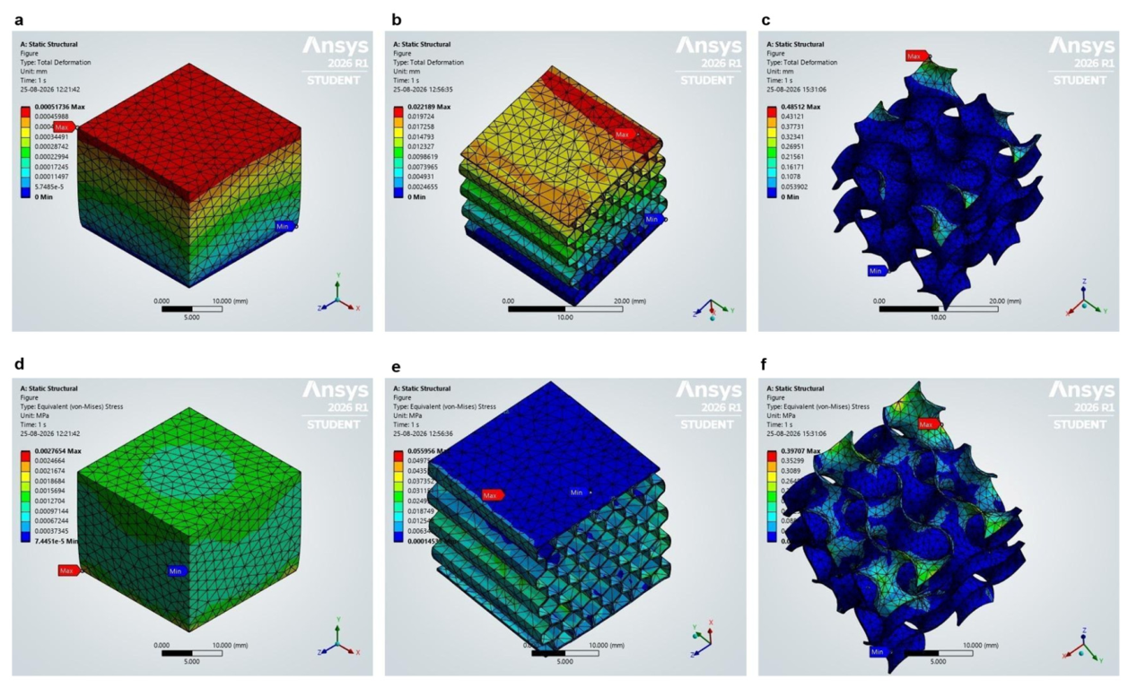
Figure 4.
Each added mass produced a distinct step in the magnetic signal. Representative raw ΔZ traces recorded by the MLX90393 for a) cast silicone b) 10% infill honeycomb c) 10% infill gyroid without a confining wall over one full load cycle from 0 to 80 g and back to 0 g in 20 g steps. Shaded bands mark the plateau at each load stage, held for about 10 s. One of three runs is shown for each skin.
Figure 4.
Each added mass produced a distinct step in the magnetic signal. Representative raw ΔZ traces recorded by the MLX90393 for a) cast silicone b) 10% infill honeycomb c) 10% infill gyroid without a confining wall over one full load cycle from 0 to 80 g and back to 0 g in 20 g steps. Shaded bands mark the plateau at each load stage, held for about 10 s. One of three runs is shown for each skin.
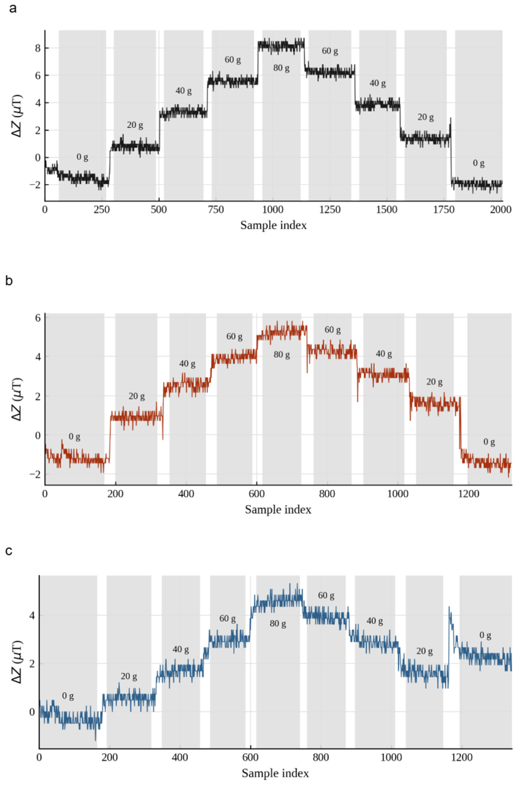
Figure 5.
Cast silicone gave the largest response at every load. Line graph of mean ΔZ ± SD across the full load sequence (0 to 80 to 0 g in 20 g steps) for all five skin configurations, n = 3 runs each. One-way ANOVA on peak response at 80 g, F(4, 10) = 117.4, p < 0.001. a) Load/unload hysteresis loops b) |Response| vs. applied mass for the loading leg c) |Response| vs. applied mass for the unloading leg.
Figure 5.
Cast silicone gave the largest response at every load. Line graph of mean ΔZ ± SD across the full load sequence (0 to 80 to 0 g in 20 g steps) for all five skin configurations, n = 3 runs each. One-way ANOVA on peak response at 80 g, F(4, 10) = 117.4, p < 0.001. a) Load/unload hysteresis loops b) |Response| vs. applied mass for the loading leg c) |Response| vs. applied mass for the unloading leg.
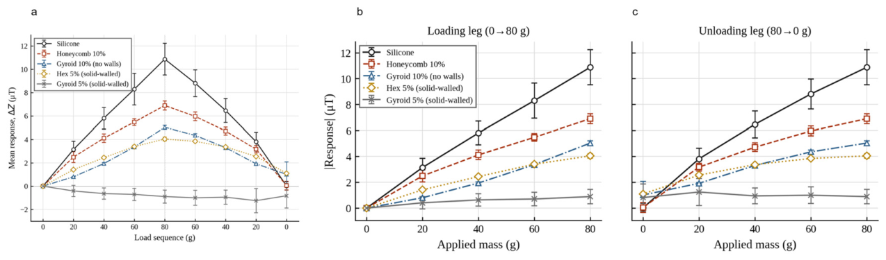
Figure 6.
Sensitivity traded off against repeatability across the five designs. Cast silicone and the 10% honeycomb had the best balance of sensitivity, hysteresis, and baseline recovery. a) Bar graph of loading-leg sensitivity (µT/g), taken as the least-squares slope of mean ΔZ versus applied mass from 0 to 80 g. The bar for the walled 5% gyroid shows the magnitude of a slightly negative slope. b) Bar graphs of intra-run noise c) inter-run repeatability d) bar graph of mean hysteresis ± SD, the absolute difference between unloading and loading responses averaged over 20, 40, and 60 g. e) bar graph of mean residual zero-load offset ± SD, the final 0 g reading minus the initial 0 g reading after one complete load and unload cycle. All panels show the five skin configurations, n = 3 runs each.
Figure 6.
Sensitivity traded off against repeatability across the five designs. Cast silicone and the 10% honeycomb had the best balance of sensitivity, hysteresis, and baseline recovery. a) Bar graph of loading-leg sensitivity (µT/g), taken as the least-squares slope of mean ΔZ versus applied mass from 0 to 80 g. The bar for the walled 5% gyroid shows the magnitude of a slightly negative slope. b) Bar graphs of intra-run noise c) inter-run repeatability d) bar graph of mean hysteresis ± SD, the absolute difference between unloading and loading responses averaged over 20, 40, and 60 g. e) bar graph of mean residual zero-load offset ± SD, the final 0 g reading minus the initial 0 g reading after one complete load and unload cycle. All panels show the five skin configurations, n = 3 runs each.
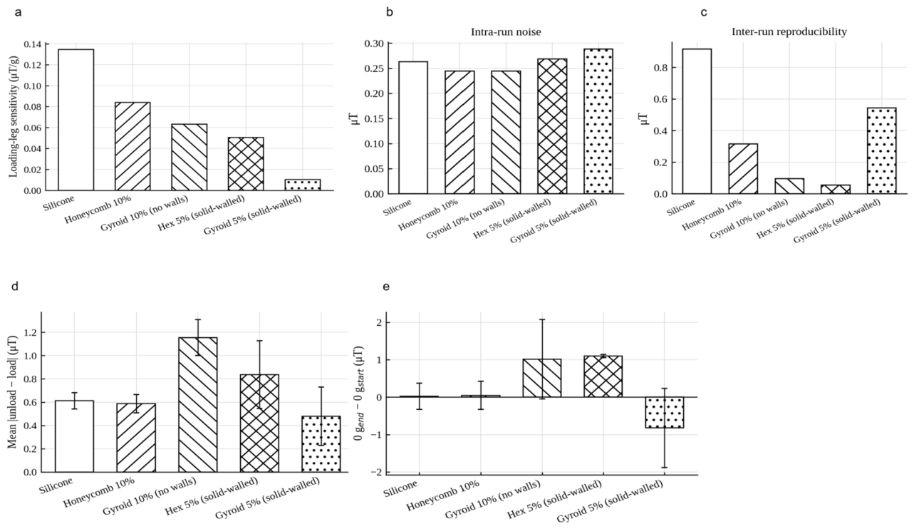

Table 1.
Simulated deformation, strain, and stress for each skin geometry. ANSYS Mechanical static structural results for 25 × 25 × 22 mm solid, honeycomb, and gyroid TPU blocks under compressive loads of 0.2 to 0.8 N applied to the top face, with the bottom face fixed. Safety factor is TPU yield strength (8.6 MPa) divided by maximum equivalent stress; ANSYS reports any safety factor above 15 as 15. Max., maximum.
Table 1.
Simulated deformation, strain, and stress for each skin geometry. ANSYS Mechanical static structural results for 25 × 25 × 22 mm solid, honeycomb, and gyroid TPU blocks under compressive loads of 0.2 to 0.8 N applied to the top face, with the bottom face fixed. Safety factor is TPU yield strength (8.6 MPa) divided by maximum equivalent stress; ANSYS reports any safety factor above 15 as 15. Max., maximum.
| Geometry | Force (N) | Max. deformation (mm) | Max. strain (mm/mm) | Max. stress (MPa) | Safety factor |
| Solid | 0.2 | 1.29×10⁻⁴ | 1.34×10⁻⁵ | 6.91×10⁻⁴ | >10 |
| Solid | 0.4 | 2.59×10⁻⁴ | 2.67×10⁻⁵ | 1.38×10⁻³ | >10 |
| Solid | 0.6 | 3.88×10⁻⁴ | 4.01×10⁻⁵ | 2.07×10⁻³ | >10 |
| Solid | 0.8 | 5.17×10⁻⁴ | 5.34×10⁻⁵ | 2.77×10⁻³ | >10 |
| Honeycomb | 0.2 | 5.55×10⁻³ | 2.57×10⁻⁴ | 1.40×10⁻² | >10 |
| Honeycomb | 0.4 | 1.11×10⁻² | 5.15×10⁻⁴ | 2.80×10⁻² | >10 |
| Honeycomb | 0.6 | 1.66×10⁻² | 7.72×10⁻⁴ | 4.20×10⁻² | >10 |
| Honeycomb | 0.8 | 2.22×10⁻² | 1.03×10⁻³ | 5.60×10⁻² | >10 |
| Gyroid | 0.2 | 0.1213 | 1.87×10⁻³ | 9.93×10⁻² | 15 |
| Gyroid | 0.4 | 0.2426 | 3.74×10⁻³ | 0.1985 | 15 |
| Gyroid | 0.6 | 0.3638 | 5.61×10⁻³ | 0.2978 | 15 |
| Gyroid | 0.8 | 0.4851 | 7.48×10⁻³ | 0.3971 | 15 |
Table 2.
Performance of each skin configuration over the full load cycle. Values from three runs of the 0 to 80 to 0 g load cycle for each skin. Peak response is mean ± SD ΔZ at 80 g. Sensitivity is the least-squares slope of the loading leg. Hysteresis is the mean absolute gap between loading and unloading responses at 20, 40, and 60 g. Residual zero-load offset is the final minus initial 0 g reading (mean ± SD). Values for the walled 5% gyroid are magnitudes of a slightly negative response. One-way ANOVA on peak response, F(4, 10) = 117.4, p < 0.001. N, number; SD, standard deviation.
Table 2.
Performance of each skin configuration over the full load cycle. Values from three runs of the 0 to 80 to 0 g load cycle for each skin. Peak response is mean ± SD ΔZ at 80 g. Sensitivity is the least-squares slope of the loading leg. Hysteresis is the mean absolute gap between loading and unloading responses at 20, 40, and 60 g. Residual zero-load offset is the final minus initial 0 g reading (mean ± SD). Values for the walled 5% gyroid are magnitudes of a slightly negative response. One-way ANOVA on peak response, F(4, 10) = 117.4, p < 0.001. N, number; SD, standard deviation.
| Configuration | N runs | Peak response @80g (µT) | Sensitivity (µT/g) | Hysteresis (µT) | Residual zero-load offset (µT) | Intra-run noise (µT) | Inter-run repeatability (µT) |
| Silicone | 3 | 10.88 ± 1.36 | 0.135 | 0.61 | 0.02 ± 0.35 | 0.26 | 0.92 |
| Honeycomb 10% (no wall) |
3 | 6.90 ± 0.38 | 0.084 | 0.59 | 0.05 ± 0.38 | 0.24 | 0.31 |
| Gyroid 10% (no wall) | 3 | 5.04 ± 0.17 | 0.063 | 1.15 | 1.02 ± 1.06 | 0.24 | 0.10 |
| Gyroid 5% (walled) | 3 | 0.89 ± 0.55 | 0.010 | 0.48 | 0.82 ± 1.06 | 0.29 | 0.54 |
| Hexagonal 5% (walled) | 3 | 4.05 ± 0.16 | 0.050 | 0.84 | 1.10 ± 0.04 | 0.27 | 0.06 |
Disclaimer/Publisher’s Note: The statements, opinions and data contained in all publications are solely those of the individual author(s) and contributor(s) and not of MDPI and/or the editor(s). MDPI and/or the editor(s) disclaim responsibility for any injury to people or property resulting from any ideas, methods, instructions or products referred to in the content. |
© 2026 by the authors. Licensee MDPI, Basel, Switzerland. This article is an open access article distributed under the terms and conditions of the Creative Commons Attribution (CC BY) license (http://creativecommons.org/licenses/by/4.0/).
Copyright: This open access article is published under a Creative Commons CC BY 4.0 license, which permit the free download, distribution, and reuse, provided that the author and preprint are cited in any reuse.