

Submitted:
28 September 2026
Posted:
29 September 2026
You are already at the latest version
Abstract
Arecanut cultivation is affected by several diseases and disorders that can reduce crop health and productivity. Automated disease identification from field images is challenging because of visually similar symptoms, illumination variations, complex backgrounds, and disease-specific texture patterns. This paper proposes a Multi-Scale Texture-Attention Network (MSTANet) for automated nine-class arecanut health and disease classification. MSTANet integrates multi-scale convolutional feature extraction, a texture-aware branch based on depthwise-separable convolutions, coordinate attention, and feature fusion to capture complementary spatial and textural characteristics. The proposed model contains 1.397 million trainable parameters and processes images resized to 150 × 150 pixels. Experiments were conducted using 5,628 images for model development and an independent test set containing 1,757 images. The model achieved 100.00% validation accuracy with a validation loss of 0.0012. On the independent test set, MSTANet achieved 88.84% accuracy, 90.55% weighted precision, 88.84% weighted recall, and 88.97% weighted F1-score. It further achieved 86.97% balanced accuracy, an MCC of 0.8669, Cohen’s kappa of 0.8643, weighted ROC-AUC of 0.9909, and weighted PR-AUC of 0.9558. The highest class-wise F1-scores were obtained for Healthy Nut (98.72%) and Mahali Koleroga (95.48%). Grad-CAM analysis was employed to provide qualitative visual explanations of model predictions and to examine the disease-relevant regions used by the network. A literature-based comparison with previously reported models addressing the same nine-class arecanut classification problem further demonstrates the competitive performance of MSTANet. The results indicate that MSTANet provides a compact, multi-scale, texture-cale feature learning, texture-aware learning, coordinate attention, explainable artificial intelligence (XAI), Grad-CAM, convolutional neural networks, precision agriculture.
Keywords:
arecanut disease classification
; multi-scale texture attention
; coordinate attention
; Grad-CAM
; precision agriculture
1. Introduction
Arecanut is a plantation crop which holds economic significance in some tropical and subtropical countries. The occurrence of fungal infections, pest attacks, stem disorders, discoloration, and other pathological conditions adversely affect plant health and productivity Zhu et al. (2026). Disease detection in conventional practices is mainly reliant on visual inspection by farmers or agronomists, which makes the entire process quite slow and prone to human error. As a result of that, image processing artificial intelligence methods have gained significant recognition in disease detection of plants Bharathi et al. (2026).
However, recent breakthroughs in the field of deep learning have shown the efficacy of convolutional neural networks (CNNs) to learn discriminative visual features from plant images directly. Recently, attention, light weight models, hybrid CNN-Transformer and graph-based learning techniques have been proposed to improve disease detection. In particular, a recent arecanut study has used graph neural network along with Bat Algorithm based hyperparameter optimization for nine-class disease classification which showed good performance on a curated dataset et al. (2026). These advancements have showcased the capability of deep learning to automate arecanut disease diagnosis process, but at the same time the need for heterogenous representation of diseases using such models have been highlighted Zeng et al. (2026).
However, there are still some challenges involved in automated arecanut health and disease classification. Firstly, arecanut diseases can happen in multiple plant organs such as leaves, nuts, trunk and foot areas. These disease manifestations have significantly different shapes, textures, colors, lesions and structures. Hence, a model built around the single plant organ is not sufficient to handle the heterogeneity of the image data. The dataset used in the present study contains nine classes comprising three healthy plant-organ categories and six disease or condition categories, thereby providing a more diverse classification problem Zhu et al. (2026).
Second, the disease symptoms may exhibit themselves at very different spatial scales. For instance, fine-scale features such as texture, fungi, small lesions, cracks, and coloration may exist alongside coarse context-dependent patterns pertaining to the diseased portion of the plant Vinutha and Prashanth (2026). However, these two different representations may not be captured by a standard convolutional network architecture. Although attention mechanisms can guide networks toward informative regions, their integration with dedicated texture learning and multi-scale feature extraction for arecanut classification remains insufficiently explored Ranganatha et al. (2026).
Thirdly, excellent predictive accuracy is not enough to prove that the model offers adequate decision-making support to agriculture. The models that are used for disease identification need to give understandable results on the areas of the image that contribute to the prediction made by the models. Methods such as Gradient-weighted Class Activation Mapping (Grad-CAM) can provide visual proof of the contributions to the prediction made by the model Sathyanarayanan et al. (2026).
In order to resolve these problems, the study puts forward a Multi-Scale Texture-Attention Network (MSTANet) for the classification of arecanut nine-class health and disease. The MSTANet uses multi-scale convolutional feature extraction and also utilizes a texture branch and coordinate attention. Multi-scale structure is intended for the capturing of disease attributes in different spatial scale, whereas the texture branch focuses on subtle surface and structural attributes. Coordinate attention follows to emphasize informative spatial representation but with maintaining spatial positioning information. These complimentary attributes are combined in the compact network with 1,397,313 trainable parameters.
This network is tested with an independent test set of 1,757 images. Besides the commonly used classification metrics, the study also considers the performance of each class, confusion pattern, prediction confidences, and Grad-CAM-based interpretability.
The main contributions of the study are as follows:
- A novel Multi-Scale Texture-Attention Network (MSTANet) is proposed for automatic nine-class arecanut disease and health status classification.
- Development of a multi-scale feature extraction module for the extraction of disease features from different spatial resolutions.
- The proposed texture-guided learning branch models the fine details of lesions and surface patterns which complement the convolutional features.
- Coordinate attention is incorporated to improve spatial feature discrimination by preserving positional information while emphasizing disease-relevant regions.
- A feature-fusion mechanism is designed to integrate multi-scale, texture, and attention features within a unified end-to-end architecture.
- Extensive experimental evaluation demonstrates the effectiveness and robustness of the proposed framework using multiple performance metrics and comparisons with state-of-the-art deep learning models.
- Grad-CAM-based visual explanations are provided to validate model decision-making and improve interpretability for practical agricultural applications.
The rest of this paper is structured as follows. In Section II, the literature review of related work in the areas of arecanut disease classification, deep learning-based plant disease detection, and explainable artificial intelligence is given. Section III covers information regarding the data used, preprocessing, and augmentation techniques. The proposed MSTANet architecture and its building blocks are presented in Section IV. Section V gives an account of the experiment results, including a detailed analysis. Section VI discusses the comparison of the proposed arecanut disease classification approach with other available approaches. Finally, Section VII concludes the study and outlines directions for future research.
2. Related Work
Recent advances in computer vision and deep learning have enabled the development of automated systems for plant disease detection and agricultural quality assessment. Research on arecanut has gradually progressed from handcrafted visual features and conventional machine learning to deep-learning-based classification, attention mechanisms, multimodal analysis, and explainable artificial intelligence (XAI). This section reviews these developments with particular emphasis on arecanut disease and quality analysis.
2.1. Traditional and Conventional Machine-Learning Methods
Early research on arecanut image analysis primarily relied on computer vision systems based on manually constructed geometric, color, texture, and defect-related features followed by conventional classifiers. These studies established the feasibility of automated arecanut classification; however, their performance depended strongly on feature selection and image acquisition conditions Shedthi Billadi et al. (2023). Such handcrafted representations may become less effective when disease symptoms exhibit high intra-class variation, multiple visual symptoms, illumination changes, or complex backgrounds.
Following handcrafted feature extraction, conventional machine-learning approaches were investigated for arecanut quality assessment and disease analysis. Bharamagoudra et al. developed an automated arecanut recognition and quality-assessment framework using feature extraction combined with CNN, SVM, and Random Forest classifiers. The approach aimed to reduce manual inspection and improve the efficiency of quality evaluation Bharamagoudra et al. (2026).
Machine learning has also been applied to weather-based arecanut disease forecasting. Lingananda et al. proposed a hybrid RF–ANN framework for forecasting Bacterial Leaf Stripe severity using weekly disease and meteorological data from Karnataka during 2019–2021. The model achieved and NRMSE of 9.2% at a two-week lead time, with maximum temperature, evening relative humidity, and rainfall identified as important predictors Lingananda et al. (2026). Similarly, Bharathi et al. investigated arecanut fruit-rot incidence using meteorological variables and evaluated Linear Regression, Random Forest, Gradient Boosting, and a Voting Regressor. The ensemble model provided the best predictive performance based on MSE and Bharathi et al. (2026). These approaches demonstrate the value of machine learning for disease forecasting; however, they depend on climatic variables rather than directly learning disease characteristics from images.
UAV and remote-sensing techniques have further expanded automated arecanut disease monitoring. Hou et al. developed an improved YOLOv10 framework for detecting areca yellowing disease from five-band multispectral UAV imagery. Using 18,520 samples, the model achieved 90.6% mAP@0.5, 91.2% precision, and 92.7% recall HOU et al. (2026). Although effective for field-level monitoring, the approach requires multispectral UAV acquisition and focuses on a specific disease rather than multi-class RGB image classification.
2.2. Deep Learning for Arecanut Disease Classification
The emergence of deep learning enabled automatic feature learning directly from arecanut images, reducing dependence on manually designed representations. Mallikarjuna et al. developed a CNN-based framework that combined multi-gradient image enhancement with AlexNet to classify normal, rot, split, and rot-split arecanut categories Gowda et al. (2026). This demonstrated the applicability of CNNs for learning disease- and defect-related visual characteristics, although the classification setting was limited to four categories.
Subsequent research investigated deeper architectures and optimization strategies. DenseNet-based approaches combined with Cuckoo Search optimization have been applied to economically important arecanut diseases, including Stem Cracking, Yellow Leaf Disease, Mahali Koleroga, and Stem Bleeding Dinesh et al. (2025). These studies demonstrate the potential of deep feature learning and optimization, but their disease settings and feature-learning strategies differ from the comprehensive nine-class classification considered in this work.
Sindhura et al. investigated ResNet50, VGG16, and EfficientNetB3 for binary classification of healthy and unhealthy arecanut leaves. The dataset was collected from the west coast of South India, with EfficientNetB3 achieving the highest reported test accuracy of 95.0% Sindhura et al. (2026). Although the study demonstrates the effectiveness of transfer-learning architectures, it is restricted to binary leaf classification and does not cover multiple diseases or different plant organs.
Pm et al. proposed Selective Kernel-DenseNet (SK-DenseNet) for arecanut disease classification. Selective-kernel operations were introduced to adapt receptive fields and capture disease characteristics at different spatial scales. The model achieved 98.92% accuracy on the Arecanut dataset and 99.99% on PlantVillage PM and Raviprakash (2026). While the adaptive receptive-field mechanism is useful for multi-scale disease patterns, the study does not specifically combine multi-scale extraction with an explicit texture branch and coordinate attention.
Shadrach et al. proposed a Graph Neural Network combined with Bat Algorithm optimization for nine-class arecanut disease detection under real-field conditions. The model used a balanced subset of 1,000 images and achieved 98.45% accuracy, 96.90% precision, 94.21% recall, and 95.05% F1-score Shadrach et al. (2026). The approach provides long-range spatial modeling; however, its evaluation was based on a balanced subset rather than the complete available dataset.
2.3. Related Arecanut Quality and Agricultural Applications
Deep learning has also been applied to arecanut ripeness and quality assessment. Aparanji et al. developed an aerial arecanut dataset and investigated AlexNet and VGG-16 for three-class ripeness classification, namely unripe, intermediate, and ripe. VGG-16 achieved 96.87% accuracy, compared with 94.58% for AlexNet Aparanji et al. (2026). Although the approach supports automated and safer harvesting, its objective is ripeness assessment rather than disease classification.
Nonglamin et al. investigated five-grade arecanut quality classification using visual characteristics such as size, shape, color, and texture. Stacking and voting ensemble-learning models were evaluated, with the proposed stacking ensemble achieving 99.00% test accuracy Nonglamin and Amitab (2026). The study demonstrates the effectiveness of visual machine learning for quality grading but does not address multi-class disease recognition across different plant organs.
Kanishka et al. presented a systematic review of arecanut post-harvest physiology, processing, value addition, by-product utilization, and emerging technologies based on 49 peer-reviewed studies. The review identified machine vision and deep-learning-based grading as promising technologies, with reported classification accuracies above 85% Kanishka et al. (2026). However, its primary focus is post-harvest processing and quality rather than automated multi-class disease identification.
Arecanut quality analysis has also been extended to multimodal imaging. Sai et al. proposed a non-destructive grading framework combining RGB surface images and X-ray radiographic images. Independent encoder fusion achieved 99.80% accuracy and 99.81% macro F1-score Sai Prashanth et al. (). Although multimodal imaging can capture both external and internal quality characteristics, it requires multiple imaging modalities and is primarily designed for quality grading rather than disease classification.
Sushitha et al. proposed a hybrid RF–attentive BiLSTM framework for agroclimatic mapping of arecanut cultivation in Central Karnataka. The model integrated nonlinear climatic relationships with temporal dependencies and achieved , RMSE of 0.39, MAE of 0.30, MAPE of 8.1%, and a correlation coefficient of 0.956 Sushitha and Aparna (2026). This work highlights the importance of climate-aware agricultural modelling but differs from image-based disease recognition.
Dai et al. developed a rapid non-destructive method for quantifying six active compounds in areca nuts using Near-Infrared Spectroscopy (NIRS) combined with PLSR and SVR. Different preprocessing and variable-selection strategies were optimized for the target compounds Dai et al. (). While useful for chemical quality assessment, the approach does not address image-based disease classification.
2.4. Deep Learning and Attention for Plant Disease Classification
Beyond arecanut-specific studies, deep learning has become an important approach for plant disease recognition because CNNs can automatically learn hierarchical visual representations. Architectures including AlexNet, VGGNet, ResNet, DenseNet, EfficientNet, and MobileNet have been widely investigated for plant disease classification under different imaging conditions Naik and Rudra (2024).
Recent studies have increasingly incorporated attention and multi-scale feature learning to improve disease representation. Attention mechanisms can emphasize informative feature regions while suppressing less relevant information, which is particularly useful when disease symptoms occupy limited image regions or when background variation affects classification Wang et al. (2025).
Lightweight architectures based on depthwise-separable convolutions have also received attention because they reduce computational requirements and model parameters, which is relevant for agricultural applications involving resource-constrained devices Naik and Rudra (2025). However, most plant disease studies focus on crops such as rice, maize, tomato, potato, and wheat. Differences in datasets, disease categories, imaging environments, and evaluation protocols also make direct cross-study comparison difficult. These observations emphasize the need for crop-specific approaches that address the visual characteristics of less extensively studied crops such as arecanut.
2.5. Explainable Artificial Intelligence in Plant Disease Diagnosis
Although deep-learning models can achieve strong classification performance, their predictions are often difficult to interpret because decision-making is distributed across learned feature representations. Explainable artificial intelligence can therefore provide additional information regarding the visual evidence underlying model predictions.
Gradient-weighted Class Activation Mapping (Grad-CAM) is a widely used visualization technique for CNN interpretation. It produces class-discriminative activation maps that highlight image regions contributing to a particular prediction. Such explanations can help determine whether the model focuses on disease-related regions rather than irrelevant background information. Therefore, incorporating visual explanation with automated classification can provide additional interpretability for agricultural decision-support applications.
2.6. Research Gap and Motivation
The reviewed studies demonstrate the potential of machine learning and deep learning for arecanut disease, health, quality, and agricultural analysis. However, several gaps remain.
First, many existing arecanut disease studies rely on conventional CNN or transfer-learning architectures with predominantly single-scale feature representations. Arecanut symptoms can appear at different spatial scales, ranging from small lesions and texture irregularities to discoloration and larger structural changes.
Second, visually similar disease categories may differ primarily in surface texture and fine-grained patterns. Explicit texture-aware representation is therefore useful for improving discrimination between closely related disease categories.
Third, although attention mechanisms and multi-scale learning have been investigated in plant disease analysis, their combined integration with an explicit texture representation and coordinate attention remains limited in arecanut-specific classification.
Fourth, several existing studies focus on individual diseases, binary classification, quality grading, or specialized imaging modalities. Comprehensive nine-class classification covering multiple healthy and diseased conditions across different arecanut plant organs remains a challenging setting.
Finally, quantitative classification performance alone does not explain which visual regions contribute to model decisions. Incorporating explainability can therefore provide complementary qualitative evidence regarding the learned representations.
Motivated by these gaps, the study proposes the Multi-Scale Texture-Attention Network (MSTANet), which integrates multi-scale feature extraction, a dedicated texture branch, coordinate attention, and feature fusion within a unified compact architecture. The framework is designed to learn complementary local, texture-based, and contextual representations for nine-class arecanut health and disease classification. Grad-CAM is additionally employed to visualize the image regions contributing to model predictions.
3. Dataset Description and Preprocessing
This section describes the arecanut image dataset used in this study, the dataset partitioning strategy, image preprocessing, and the training-time data augmentation procedure adopted before feeding the images to the proposed MSTANet model.
3.1. Dataset Description
This study utilizes a multi-class arecanut image dataset containing healthy and diseased samples representing different plant organs and anatomical regions. The considered conditions include leaf, nut, trunk, stem, and foot regions of the arecanut plant. Consequently, the dataset contains considerable visual variation in terms of texture, color, structural appearance, lesion characteristics, and disease manifestation.
The dataset consists of nine health and disease classes:
- 1.
- Healthy Leaf
- 2.
- Healthy Nut
- 3.
- Healthy Trunk
- 4.
- Mahali Koleroga
- 5.
- Stem Bleeding
- 6.
- Bud Borer
- 7.
- Healthy Foot
- 8.
- Stem Cracking
- 9.
- Yellow Leaf Disease
The nine-class formulation enables the proposed framework to distinguish both healthy plant conditions and different disease- or pest-related conditions. The class mapping implemented in the experimental framework contains nine output categories corresponding to these conditions.
It is important to note that the reason for choosing a nine-class setting is to reflect the various health conditions of arecanut plants, which occur in different plant organs such as leaves, nuts, trunks, and foot area. The reason for including several healthy and diseased conditions rather than limiting the analysis to one disease condition is due to differences in the appearance of each condition in color and structure.
Representative samples from the nine classes are presented in Figure 1.
3.2. Dataset Partitioning
The dataset used for model development contains 5,628 images. These images were divided into training and validation subsets using an 80:20 partition, resulting in 4,502 training images and 1,126 validation images. An additional independent test dataset containing 1,757 images was used exclusively for final model evaluation.
The dataset organization used in the experiments is summarized in Table 1.
The training and validation subsets were used during model development, whereas the independent test set was reserved for final performance assessment. The test samples were not used during model training or model selection.
3.3. Image Preprocessing
Before being supplied to MSTANet, all input images were resized to a fixed spatial resolution of pixels. The images were converted into tensors and normalized using the channel-wise statistics adopted in the implementation. The resulting input consists of three-channel RGB images with a spatial resolution of pixels.
The normalization operation is defined as
where I represents the input image, denotes the channel-wise mean, and represents the corresponding channel-wise standard deviation.
The normalization parameters used in the experiments are
and
These transformations provide a consistent input representation for the network.
3.4. Training Data Augmentation
Data augmentation technique was used for the training images to add more variability during the model training process. Augmentation was used only for the training set while validation and testing samples were not augmented.
The used training pipeline consists of image resizing, random horizontal flipping, random vertical flipping, random rotation, and brightness, contrast, and saturation variation using ColorJitter. The augmentation operations and their corresponding settings are summarized in Table 2.
The horizontal and vertical flipping operations introduce variations in image orientation, while random rotation provides moderate geometric variation. Brightness, contrast, and saturation perturbations modify image appearance and provide additional variation during training.
3.5. Evaluation Preprocessing
Random augmentations were not performed during the validation and testing phases. The validation and testing pictures were scaled to the desired input resolution and normalized the same way the input was.
This makes sure that the validation and test results presented are computed based on the specified evaluation set without any random augmentations from the training phase.
3.6. Preprocessing Pipeline
The complete preprocessing procedure can be summarized as
where is applied only to the training images. For validation and test images, the augmentation stage is omitted. The prepared images are subsequently supplied to the proposed model.
4. Proposed Multi-Scale Texture-Attention Network
This section introduces the MSTANet architecture for nine-class classification of arecanut health and disease conditions. The model is designed to learn complementary visual representations from arecanut images with various disease indications present in different plant organs. These disease indications could be in the form of discolourations, lesions, fungal patterns, stem bleedings, cracks, pest damage, and other forms of structural damage.
In this regard, the proposed network learns multi-scale features, texture features, coordinate attention, and feature fusion in a compact CNN architecture. The overall architecture of MSTANet is illustrated in Figure 2.
4.1. Overall Architecture
The input to MSTANet is an RGB image resized to pixels. The input tensor is therefore represented as
The network gradually converts the image to increasingly discriminative features. The main stages involved include feature extraction using convolutions, multiscale features learning, texture-based features extraction, coordinate attention, feature fusion, global features aggregation, and finally classification.
The overall transformation is represented as
where denotes multi-scale feature extraction, represents texture-aware feature extraction, denotes coordinate attention, represents feature fusion, denotes global feature aggregation, and represents the classification head.
4.2. Initial Feature Extraction
The first stage of MSTANet extracts low-level visual representations from the input image using convolutional operations. For an input feature map , a convolutional transformation can be expressed as
where W represents the convolutional kernel, denotes the bias associated with the k-th output channel, and represents the nonlinear activation function.
The resulting feature maps provide the fundamental representations used by the subsequent multi-scale and texture-aware branches.
4.3. Multi-Scale Feature Extraction
Arecanut disease symptoms can exhibit considerable variation in spatial size. Small lesions, cracks, and fungal structures may coexist with larger regions of discoloration or structural abnormalities. A single receptive-field scale may therefore be insufficient to represent all relevant disease characteristics.
MSTANet addresses this issue using multi-scale feature extraction. Given an intermediate feature representation , multiple feature transformations are applied to obtain complementary representations:
where denotes the feature transformation associated with the corresponding scale, denotes feature concatenation, and denotes the subsequent feature-processing operation.
The multi-scale representation enables the network to jointly preserve local disease characteristics and broader contextual information.
4.4. Texture-Aware Feature Learning
Texture is very significant in diagnosing several arecanut diseases. Various parameters such as roughness of surface, lesion edges, fungal infection, bleeding and cracking are some of these factors.
To explicitly represent these characteristics, MSTANet incorporates a dedicated texture-aware feature-learning branch. The texture representation is expressed as
where denotes the texture feature-learning operation.
The texture representation complements the broader contextual information learned by the multi-scale branch. The two representations are subsequently combined as
where ∥ denotes feature concatenation.
This complementary representation allows the network to jointly exploit spatial context and fine-grained texture characteristics.
4.5. Coordinate Attention Mechanism
Following multi-scale and texture-aware feature extraction, MSTANet employs coordinate attention to enhance informative spatial representations.
Let denote the combined feature representation. The coordinate-attention operation can be represented as
where denotes the coordinate-attention operation.
The attention-refined representation is obtained as
where ⊙ denotes element-wise multiplication.
The attention mechanism enables the network to assign greater importance to informative regions while reducing the influence of less relevant visual information. This is particularly useful when disease symptoms occupy only a portion of the image.
4.6. Feature Fusion
The multi-scale and texture-aware representations are integrated before the final classification stage. Feature fusion produces a combined representation containing complementary contextual, spatial, and texture information.
The fusion operation is represented as
where denotes the feature-fusion and refinement operation.
The fused representation provides the classification head with a richer feature space than would be obtained from an individual feature branch.
4.7. Global Feature Aggregation
The spatial feature maps produced after feature fusion are converted into a compact feature vector using global average pooling. For a feature map with spatial dimensions , the pooled representation for channel c is calculated as
Global feature aggregation reduces the spatial dimensionality of the representation while retaining the overall response of each feature channel. The resulting feature vector is subsequently provided to the classification layer.
4.8. Nine-Class Classification
The final classification layer produces nine output logits corresponding to the nine arecanut categories considered in this study. The softmax function converts these logits into class probabilities:
The predicted class is determined according to
The nine classes are Healthy Leaf, Healthy Nut, Healthy Trunk, Mahali Koleroga, Stem Bleeding, Bud Borer, Healthy Foot, Stem Cracking, and Yellow Leaf Disease.
4.9. Model Complexity
The proposed MSTANet can be regarded as a lightweight convolutional network with multiple feature-learning methods. There are 1,397,313 learnable parameters in the implemented network.
The smaller number of parameters is beneficial for deploying the model to limited-resource agricultural environment. The complexity of MSTANet model will be then discussed in the next section along with classification performance.
4.10. Training Configuration
MSTANet was trained based on the experimental setting for the main experiment. It was trained with AdamW optimization and the same loss function as in the case of the MSTANet experiment. Early stopping was implemented in order to stop the unnecessary optimization, as soon as the validation performance stopped improving.
The training process evaluated the validation performance and kept the best performing model. This was the model that was used to evaluate the performance on the test set.
The principal training configuration is summarized in Table 3.
The specific values of the learning rate, weight decay, batch size, the maximum number of epochs, and early stopping patience should be stated based on the actual MSTANet training setup used for obtaining the results.
4.11. Explainability Through Grad-CAM
In order to offer a qualitative perspective on how the MSTANet makes decisions, Grad-CAM is utilized after the training process of the model. Grad-CAM generates class-specific activation maps of the input image regions responsible for the chosen prediction.
For a target class c, the importance weight of feature channel k can be represented as
where denotes the score for class c and represents the k-th feature map of the selected convolutional layer.
The Grad-CAM activation map is then calculated as
These activation maps are displayed as heat maps and superimposed on the respective input images. These visualizations provide qualitative evidence of the spatial regions contributing to MSTANet predictions and are presented in Section V.
5. Experimental Results and Discussion
The section describes the experimental evaluation of the proposed MSTANet for arecanut health and disease classification using nine classes. The investigation involves the study of the training behavior, general performance on the independent test data, class-level classification performance, confusion matrix analysis, generalization behavior, prediction confidence, and interpretability via Grad-CAM method.
All test performance values are derived using the independently kept test set that consists of 1,757 images. The trained model, which is selected during training process, is loaded before conducting the final test performance evaluation.
5.1. Experimental Configuration
The proposed MSTANet was implemented using PyTorch and trained using a CUDA-enabled computational environment. The model accepts RGB images of size pixels and produces predictions for nine classes. The implemented network contains 1,397,313 trainable parameters.
A batch size of 32 was used for model training and evaluation. The AdamW optimizer was employed with an initial learning rate of 0.001 and a weight decay of 0.0001. Cross-entropy loss was used for the multi-class classification task. A cosine annealing learning-rate scheduler was adopted to progressively reduce the learning rate during training.
The maximum number of training epochs was set to 40. Early stopping was configured with a patience of seven epochs and a minimum validation-loss improvement of 0.001. The training configuration is summarized in Table 4.
The model successfully produced an output tensor of dimensions for an input batch of dimensions , confirming the expected nine-class output configuration.
5.2. Evaluation Metrics
The performance of MSTANet was evaluated using multiple complementary metrics rather than relying only on overall accuracy. Accuracy measures the proportion of correctly classified samples and is defined as
Precision and recall are defined as
and
The F1-score provides the harmonic mean of precision and recall:
For the reported multi-class results, precision, recall, and F1-score were calculated using weighted averaging according to class support. Balanced accuracy was additionally used to account for differences in class representation.
The Matthews correlation coefficient (MCC) and Cohen’s kappa were included to provide additional measures of agreement between predicted and ground-truth labels. ROC-AUC was calculated using a weighted one-vs-rest strategy, while PR-AUC was calculated using weighted averaging of the class-wise precision-recall information.
These metrics were implemented directly in the final evaluation pipeline.
5.3. Training Performance
MSTANet was trained for a maximum of 40 epochs with early stopping. The training process monitored training loss, validation loss, training accuracy, and validation accuracy at every epoch.
Although training was allowed to continue until the stopping criterion was reached, the best model selected according to the implemented validation criterion corresponded to epoch 33. At this epoch, MSTANet achieved a validation accuracy of 100.00% and a validation loss of approximately 0.0012. The corresponding training accuracy and training loss were 99.58% and 0.0166, respectively.
Training eventually reached epoch 40, where the early-stopping criterion was triggered. However, the previously stored best model corresponding to epoch 33 was restored for subsequent evaluation. The total training time was 164.67 minutes.
The training summary is presented in Table 5.
Figure 3 presents the training and validation curves generated during model optimization.
The training curves provide an indication of the optimization behavior of the proposed network. The progressive reduction in training and validation loss demonstrates convergence of the optimization process, while the corresponding accuracy curves illustrate the improvement in classification performance during training.
5.4. Performance Across Dataset Splits
To assess the relationship between model-development performance and independent evaluation performance, the accuracy and loss obtained from the training, validation, and test sets were compared.
Table 6 summarizes the performance across the three dataset splits.
Figure 4 illustrates the classification accuracy across the training, validation, and independent test sets.
The training-to-test accuracy difference is approximately 10.73 percentage points, while the validation-to-test difference is approximately 11.16 percentage points. This indicates a measurable generalization gap between the development data and the independent test set.
The training-to-test accuracy difference is approximately 10.73 percentage points, while the validation-to-test difference is approximately 11.16 percentage points. This indicates a measurable generalization gap between the development data and the independently held-out test data.
Although MSTANet achieved nearly perfect validation performance, the independent test accuracy of 88.84% provides a more realistic indication of performance on unseen samples. The observed gap may be associated with differences in image characteristics, class representation, and the complexity of visually similar arecanut conditions.
Therefore, the 100.00% validation accuracy should not be interpreted as perfect generalization. The independent test results are used as the primary basis for assessing the effectiveness of MSTANet.
5.5. Overall Test Performance
The final MSTANet model was evaluated on an independent test set containing 1,757 images. The model generated a probability matrix of dimensions , corresponding to the nine output classes. Table 7 presents the overall test performance.
MSTANet achieved an overall accuracy of 88.84% and a weighted F1-score of 88.97%. The weighted precision was slightly higher at 90.55%, indicating that the predicted classes were generally reliable with respect to the weighted class distribution.
The balanced accuracy of 86.97% provides an additional indication of performance when considering the contribution of individual classes. Furthermore, the MCC and Cohen’s kappa values of 0.8669 and 0.8643, respectively, indicate strong agreement between predicted and ground-truth labels.
The weighted ROC-AUC of 0.9909 demonstrates strong class separability based on the predicted probabilities. The weighted PR-AUC of 0.9558 further indicates strong precision-recall behavior across the nine classes.
5.6. Class-Wise Classification Performance
Overall metrics can conceal differences in the recognition of individual disease and healthy categories. Therefore, class-wise precision, recall, F1-score, and support were calculated on the independent test set.
The complete class-wise results are presented in Table 8.
Healthy Nut achieved the strongest overall class-wise performance, with precision, recall, and F1-score values of 0.9936, 0.9809, and 0.9872, respectively. Mahali Koleroga also showed strong recognition, achieving an F1-score of 0.9548 and a recall of 1.0000.
Healthy Trunk achieved a precision of 1.0000, although its recall was 0.7465, indicating that some samples belonging to this class were assigned to other categories. Yellow Leaf Disease obtained a recall of 0.9216, indicating that most of its test samples were correctly identified.
The lower F1-score obtained for Bud Borer indicates greater difficulty in distinguishing this category from visually similar classes. Healthy Foot also obtained an F1-score of 0.6000; however, only three test images belonged to this category. Therefore, the corresponding class-wise metric should be interpreted cautiously because of the extremely small test support.
The class-wise results demonstrate that the model does not perform uniformly across all categories, emphasizing the importance of reporting both aggregate and class-specific metrics.
5.7. Confusion Matrix Analysis
The confusion matrix provides a detailed view of the classification patterns across the nine categories. Figure 5 presents the confusion matrix obtained from the independent test set.
The confusion matrix shows strong recognition for several classes. All 317 Mahali Koleroga samples and all 28 Stem Bleeding samples were correctly classified. Similarly, 463 out of 472 Healthy Nut samples were correctly identified.
Healthy Trunk exhibited several misclassifications, with the largest number of errors involving Yellow Leaf Disease. Yellow Leaf Disease also showed confusion with Healthy Leaf and Stem Bleeding. Such errors suggest that some categories exhibit overlapping visual characteristics.
Bud Borer also showed confusion with Healthy Leaf, Healthy Nut, and Yellow Leaf Disease. Stem Cracking exhibited misclassifications involving Mahali Koleroga, Bud Borer, Healthy Foot, and other categories.
These observations indicate that fine-grained arecanut disease recognition remains challenging when different conditions exhibit similar color, texture, or structural characteristics. The confusion matrix therefore complements the aggregate metrics by identifying the specific categories where additional feature discrimination may be beneficial.
5.8. Prediction Confidence Analysis
In addition to classification performance, the prediction confidence of MSTANet was examined using the maximum predicted class probability for each test sample. The analysis was performed on all 1,757 test images.
The mean prediction confidence over the test set was 97.01%. Correctly classified samples had a mean confidence of 99.15%, whereas incorrectly classified samples had a mean confidence of 79.94%.
Figure 6 presents the distribution of confidence values for correct and incorrect predictions.
The prediction confidence distribution provides additional insight into the decision behavior of MSTANet. As shown in Figure 6, correct predictions exhibit a highly concentrated confidence distribution near unity, whereas incorrect predictions demonstrate substantially greater variability. The mean confidence for correct predictions was 99.15%, compared with 79.94% for incorrect predictions.
The lower confidence and wider distribution observed for incorrect predictions indicate that prediction uncertainty tends to increase when the model encounters visually ambiguous samples. Nevertheless, the presence of high-confidence incorrect predictions also indicates that confidence alone cannot be considered a definitive measure of prediction correctness.
5.9. Class-Wise Prediction Confidence
To further investigate the confidence behavior of the model, the mean prediction confidence was calculated separately for each class.
The class-wise confidence values are reported in Table 9.
Figure 7 presents the class-wise prediction confidence.
The highest mean confidence values were obtained for Stem Bleeding, Mahali Koleroga, and Healthy Nut. In contrast, Healthy Foot exhibited the lowest mean confidence. The lower confidence for Healthy Foot should be interpreted together with its extremely small test support of only three samples.
The confidence analysis therefore provides an additional perspective on the behavior of the classifier, complementing the conventional classification metrics.
5.10. Generalization Analysis
The comparison between training, validation, and independent test performance reveals a noticeable difference between development-set and test-set accuracy. The training-to-test accuracy gap is 10.73 percentage points, while the validation-to-test gap is 11.16 percentage points.
Although the validation accuracy reached 100.00%, the independent test accuracy was 88.84%. This difference indicates that the validation result should not be interpreted as evidence of perfect generalization.
The observed generalization gap may be influenced by differences between the development and test samples, variations in disease appearance, and the uneven representation of some categories. In particular, several classes have substantially different support values in the independent test set.
Consequently, the independent test accuracy and the corresponding multi-metric evaluation provide the primary evidence for assessing the practical performance of MSTANet.
Future experiments should investigate larger and more diverse field-acquired datasets, cross-dataset validation, and domain generalization strategies to further assess the robustness of the proposed architecture.
5.11. Grad-CAM-Based Explainability Analysis
To examine the spatial information contributing to MSTANet predictions, Gradient-weighted Class Activation Mapping (Grad-CAM) was applied to the feature-fusion layer.
The selected target layer was the first layer of the feature-fusion module, corresponding to a convolution that transforms the 192-channel feature representation into 256 channels.
For a target class c, the importance weight of feature map k is computed as
where represents the k-th activation map and denotes the model score for class c.
The Grad-CAM localization map is obtained using
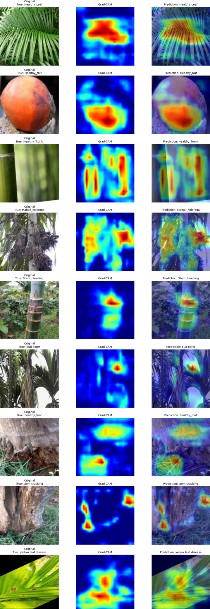
The generated activation maps were upsampled to the original input-image resolution and normalized before visualization to facilitate intuitive interpretation of the model’s decision-making process. Figure 8 presents representative Grad-CAM visualizations obtained from correctly classified samples across all nine arecanut health and disease categories. For each class, the first column shows the original input image, the second column presents the corresponding Grad-CAM activation map, and the third column shows the heatmap overlaid on the original image. The highlighted regions indicate the image areas that contribute most strongly to the final classification decision
The Grad-CAM visualizations provide qualitative evidence regarding the regions utilized by MSTANet during classification. For healthy samples, the network primarily focuses on characteristic structural components such as leaf blades, nut surfaces, trunk textures, and foot regions. Similarly, for diseased samples, the model attends to symptom-bearing areas associated with infection, discoloration, pest damage, stem bleeding, trunk cracking, and other disease-specific visual patterns. The overlay visualizations demonstrate that the activated regions are generally concentrated around biologically meaningful structures rather than irrelevant background areas. This behavior suggests that MSTANet learns disease-relevant representations and effectively localizes discriminative visual cues required for accurate classification. Furthermore, the consistency of the activation patterns across multiple classes provides additional confidence in the reliability and interpretability of the proposed framework. The observed attention maps indicate that the network predominantly relies on symptom-related image regions when generating predictions, thereby reducing the likelihood of spurious background-driven decisions. It should be noted that the present dataset does not contain pixel-level disease annotations. Therefore, the Grad-CAM analysis serves as a qualitative interpretability assessment rather than a quantitative localization evaluation. Nevertheless, the visual explanations provide valuable insight into the internal decision-making process of MSTANet and support the practical applicability of the proposed model for explainable arecanut disease diagnosis.
5.12. Model Complexity
The proposed MSTANet contains 1,397,313 trainable parameters. The model receives an input tensor of dimensions for a batch size of 32 and produces a nine-dimensional output for each image.
The relatively compact parameter count results from the use of depthwise-separable convolutional operations together with progressive feature extraction and attention-based refinement.
Table 10 summarizes the basic computational configuration of the implemented network.
Figure 8.
Grad-CAM explanations of MSTANet across the nine arecanut classes.
The parameter count demonstrates that MSTANet maintains a relatively compact architecture while incorporating multi-scale processing, texture representation, and coordinate attention.
5.13. Discussion of Experimental Findings
The experimental results demonstrate that MSTANet can effectively distinguish multiple healthy and diseased arecanut conditions using a single unified classification framework.
The overall test accuracy of 88.84% and weighted F1-score of 88.97% indicate strong classification capability across the evaluated dataset. The high weighted ROC-AUC of 0.9909 further demonstrates strong probability-based class separability.
The class-wise results, however, reveal that performance is not uniform across all categories. Healthy Nut and Mahali Koleroga are recognized particularly well, whereas Bud Borer presents a more challenging classification problem. The extremely small support of the Healthy Foot class also limits the reliability of its class-specific performance estimate.
The confusion matrix indicates that several errors occur between categories with visually overlapping characteristics. This observation supports the motivation for combining multi-scale and texture-aware feature learning with spatial attention.
The confidence analysis further shows that correct predictions generally receive substantially higher confidence than incorrect predictions. Finally, Grad-CAM provides a visual mechanism for examining the regions contributing to model decisions.
Taken together, the results indicate that MSTANet provides a useful combination of classification performance, compact model design, and qualitative interpretability. Nevertheless, the observed validation-to-test performance gap indicates that further evaluation on larger and more diverse datasets is necessary before making claims about broad field-level generalization.
5.14. Summary of Experimental Findings
The final MSTANet evaluation on the independent test set demonstrated an accuracy of 88.84%, weighted precision of 90.55%, weighted recall of 88.84%, and weighted F1-score of 88.97%. The model additionally achieved a balanced accuracy of 86.97%, MCC of 0.8669, Cohen’s kappa of 0.8643, weighted ROC-AUC of 0.9909, and weighted PR-AUC of 0.9558.
Class-wise analysis showed particularly strong performance for Healthy Nut and Mahali Koleroga, while Bud Borer remained comparatively challenging. Healthy Foot should be interpreted cautiously because only three test samples were available for this category.
The confusion matrix demonstrated that classification errors were mainly associated with categories exhibiting overlapping visual characteristics. The generalization analysis revealed an 11.16 percentage-point gap between validation and independent test accuracy, emphasizing the importance of independent evaluation.
The confidence analysis showed a mean confidence of 97.01% across the test set, with higher confidence for correct predictions than for incorrect predictions. Finally, Grad-CAM visualization provided qualitative evidence for examining the spatial information contributing to the model predictions.
Overall, the experimental results support the effectiveness of MSTANet as a compact multi-scale, texture-aware, and attention-guided framework for nine-class arecanut health and disease classification. Further experiments involving ablation studies, comparisons with established deep learning models, and evaluation on additional datasets are required to isolate the contribution of each architectural component and establish the relative advantage of the proposed framework.
6. Comparative Analysis
To further assess the effectiveness of the proposed MSTANet architecture, a literature-based comparative analysis was conducted with previously reported deep-learning approaches for arecanut disease classification. Particular emphasis was given to studies addressing the same nine-class arecanut classification problem. The comparison considers the reported dataset size, data augmentation strategy, test-set configuration, and test accuracy.
Published studies may differ in dataset partitioning, preprocessing, augmentation strategy, model architecture, and evaluation protocol. Therefore, the reported results are used for contextual comparison rather than as a direct controlled benchmark. The independent test performance obtained by MSTANet in the present study remains the primary basis for evaluating the proposed framework.
6.1. Comparison with Previously Reported Nine-Class Methods
Several recent studies have investigated deep-learning approaches for multi-class arecanut disease classification. Among the reported methods, EfficientNet-B0, MobileNetV3Small, and DenseNet-inspired CNN architectures have been evaluated for the nine-class arecanut classification problem.
The comparison is summarized in Table 11.
Here, “NR” denotes that the corresponding information was not explicitly reported in the respective study. For MSTANet, augmentation was performed online during training; therefore, no additional augmented image files were generated. Augmentation was applied exclusively to the training subset, while validation and independent test images were not augmented.
The comparison indicates that MSTANet achieved a test accuracy of 88.84%, which is higher than the reported test accuracies of EfficientNet- B0 (58.38%), MobileNetV3Small (83.87%), and the DenseNet-inspired CNN with a growth rate of 16 (87.87%). The result demonstrates the competitiveness of the proposed architecture among the selected previously reported methods with lower test accuracy.
However, some recently reported approaches achieved higher accuracy, including the GNN–Bat Algorithm model (98.45%) and MobileNetV3Small-CM FusionNet (99.54%). These results should be interpreted cautiously because the studies employ different dataset compositions, preprocessing procedures, augmentation configurations, and evaluation protocols. Consequently, the reported accuracy values do not constitute a controlled same-dataset benchmark.
From the above analysis, it is evident that the proposed MSTANet is a very balanced network in terms of classification ability, architecture compactness, and feature representation. While most other approaches focus solely on one of these three aspects, for instance on a feature representation approach or hand-crafted descriptors or multi-modal images, the proposed MSTANet integrates the aspects of multi-scale feature extraction, texture-aware learning, and coordinate attention in a compact architecture. This model is able to represent both detailed and spatial features through 1.397 million learnable parameters.
6.2. Dataset and Augmentation Comparison
This dataset setting plays a crucial role in analyzing the classification outcomes presented here. As the previous techniques relied on a larger dataset of 11,063 images, in the current study, 5,628 images have been employed for training, while 1,757 have been used for testing purposes.
As regards the present architecture, the augmentation process occurs only during training in an online way; hence, the total number of images does not change. Validation and test data sets remain intact and are not subject to stochastic augmentation in order to evaluate the generalization performance of the models.
In contrast, the exact count of augmented images used in previous studies is unknown. Hence, “NR” stands instead of the estimation of this value based on the size of the reported datasets.
6.3. Analysis of Comparative Performance
Table 11 presents a comparison between the proposed MSTANet and previously reported deep-learning models evaluated for the same nine-class arecanut disease classification problem. MSTANet achieved an independent test accuracy of 88.84%, which is higher than the reported test accuracies of EfficientNet-B0 (58.38%), MobileNetV3Small (83.87%), and the DenseNet-inspired CNN with a growth rate of 16 (87.87%) Dinesh (2025).
The comparison becomes especially important because the compared methods deal with the same nine classes of arecanut. Nevertheless, the experimental setups used are not identical. In the former study, there were 11,063 images, out of which 1,550 images comprised the testing dataset. In the present study, there were 5,628 images used for training, along with a test dataset of 1,757 images.
These results suggest that the performance of MSTANet is comparable to the other previously studied networks. The proposed network is tailored to perform multi-scale feature extraction, texture-aware representation, coordinate attention, and feature fusion to extract complementary features of the disease in arecanut organs.
6.4. Comparison with Higher-Performing Reported Methods
Although MSTANet outperformed the selected lower-performing models included in Table 11, some models reported in the same literature achieved higher test accuracies. In particular, the baseline CNN and the MobileNetV3Small-CM FusionNet reported test accuracies of 93.74% and 99.54%, respectively Dinesh (2025).
These results are acknowledged to provide a balanced assessment of the relative performance of MSTANet. However, the reported values were obtained under the experimental configuration of the corresponding study and were not reproduced using the independent 1,757-image test set adopted in the present work. Therefore, these values should not be interpreted as results from a controlled head-to-head experiment.
Rather, the comparison highlights the fact that the performance of the MSTANet is within the acceptable range for the same nine-class arecanut classification task in terms of the results that have been reported before. Test performance metrics and Grad-CAM visualization provide another perspective to evaluate the proposed architecture.
6.5. Dataset and Augmentation Comparison
The dataset and augmentation configurations provide important context for interpreting the comparative results. The previously reported study used a dataset containing 11,063 images and evaluated the models on a 1,550-image test set. In contrast, the present study used 5,628 images for model development and an independent test set of 1,757 images.
For MSTANet, data augmentation was performed online and exclusively on the training subset. Consequently, augmentation does not increase the number of stored training images. Validation and independent test images were not subjected to stochastic augmentation, thereby preserving an unmodified evaluation set.
The exact number of augmented images generated by the previously reported methods was not explicitly specified. Therefore, the augmentation-count field is reported as “NR” in Table 11 rather than estimating the number of generated samples.
6.6. Summary of Comparative Findings
Overall, the literature-based comparison demonstrates that MSTANet achieves competitive performance for the same nine-class arecanut disease classification problem. Its independent test accuracy of 88.84% exceeds the reported results of the selected EfficientNet-B0, MobileNetV3Small, and DenseNet-inspired CNN configurations.
At the same time, the higher reported performance of the baseline CNN and MobileNetV3Small-CM FusionNet is acknowledged, avoiding an overstatement of the comparative advantage of MSTANet. Differences in dataset partitioning and experimental protocols should be considered when interpreting these cross-study results.
The proposed MSTANet further provides a compact architecture integrating multi-scale learning, texture-aware representation extraction, and coordinate attention, together with comprehensive evaluation and Grad-CAM-based interpretability analysis. These characteristics position MSTANet as a competitive and explainable framework for automated nine-class arecanut health and disease classification.
7. Conclusion and Future Work
The research article described MSTANet, a small Multi-Scale Texture-Attention Network designed for automated recognition and classification of nine classes of arecanut health and disease status.
According to the experimental results, MSTANet can successfully differentiate between healthy and diseased conditions of different arecanut plant organs. The evaluation through an independent testing set, the analysis of the accuracy rates per class, and confusion matrix results show high recognition rates for nine classes considered. Moreover, the analysis performed with the help of Grad-CAM helped to prove that MSTANet can focus on the relevant parts of arecanut images indicating diseases.
A literature-based comparative study with existing approaches to nine-class classification of arecanuts showed that MSTANet has a good performance. The developed network yielded 88.84% accuracy on the independent test set, which includes 1,757 images. Though some of the existing approaches outperformed the proposed approach in terms of test accuracy, their performance was measured using other configurations of the dataset. It was found that there is a certain generalization gap between the development and the independent test sets. Thus, the necessity of using a large number of samples for development and testing was confirmed.
Future work will focus on collecting large and varied datasets through field experimentation, balancing classes and generalizing across domains, as well as extending the framework to severity assessment and symptom localization. Light-weight CNN-Transformer models, cross-dataset testing, and edge computing will also be explored.
In summary, the MSTANet model offers a concise, multi-scale, texture-based, and interpretable system for classifying arecanut plant health and diseases into nine different categories. More extensive field and cross-disciplinary evaluations will need to be conducted to confirm this.
Funding
The authors received no financial support or funding for the research, authorship, or publication of this article.
Institutional Review Board Statement
The study did not involve human participants, human data, or animals. Therefore, ethical approval was not required.
Data Availability Statement
The arecanut image dataset used in this study is publicly available through the Kaggle repository, “Arecanut Dataset,” maintained by TejPAVIraj. The dataset can be accessed at: https://www.kaggle.com/datasets/tejpaviraj/arecanut. The data are publicly available subject to the terms and conditions of the Kaggle repository.
Conflicts of Interest
The authors declare that they have no conflict of interest.
References
- Zhu, H.; Mehmood, S.; Liu, L. First Report of Leaf Sheath Rot of Arecanut (Areca catechu) Caused by Marasmiellus palmivorus in China. Plant Disease 2026, pp. PDIS–07.
- Bharathi, K.; Ashwini, B.; Shrikanth Rao, S.; Prathibha, V. Hybrid Spatio-temporal Deep Learning Framework for Early Prediction of Arecanut Fruit Rot Disease 2026.
- et al., F.D.S. Arecanut disease detection using graph neural networks and Bat Algorithm optimization. Scientific Reports 2026, 16, 15785. [CrossRef]
- Zeng, W.; He, X.; Peng, X.; Yu, Z.; Li, J.; Wang, L. Fungal Diversity, Pathogenic Characteristics and Fungicide Sensitivity of Pathogens Isolated from Areca catechu L. Diseases in Hainan Island. Agronomy 2026, 16, 671.
- Vinutha, H.; Prashanth, G. Areca Nut Disease Classification Using Sailfish Optimization Algorithm with Dynamic Elastic Boundary Strategy and Convolution Neural Networks. Engineering, Technology & Applied Science Research 2026, 16, 37394–37401.
- Ranganatha, Y.; Killedar, F.D.; Devraj, G. Koleroga (Mahali): The Silent Destroyer of Arecanut 2026.
- Sathyanarayanan, P.M.; Bharathy, P.; Mohan, M.; Munawar, M.A.; Priya, S.; et al. EXPLORING THE COMBINED USE OF ARECA NUT AND TOBACCO: FROM TRADITIONAL PRACTICES TO MODERN PUBLIC HEALTH CONCERNS. Genetics and Molecular Research 2026.
- Shedthi Billadi, S.; Siddappa, M.; Shetty, S.; Shetty, V. Classification of arecanut using machine learning techniques. International Journal of Electrical and Computer Engineering 2023, 13, 1914–1921. [CrossRef]
- Bharamagoudra, P.; Bharamagoudar, G.R.; et al. Areca Nut Recognition Using Machine Learning. In Proceedings of the 2026 4th International Conference on Knowledge Engineering and Communication Systems (ICKECS). IEEE, 2026, pp. 1–6.
- Lingananda, N.K.; Naik, G.B.; Chittaragi, A.; Patil, B.; Shankarappa, S.; Vasanad, N.C.; Patil, S.; Naik, M.K. Hybrid machine learning framework for predicting bacterial leaf stripe disease in arecanut under complex agroclimatic conditions. Microbial Risk Analysis 2026, p. 100371.
- Bharathi, K.; Ashwini, B.; Rao, S.S.; Prathibha, V. Machine Learning Approaches for Correlation Analysis of Arecanut Fruit Rot Disease Intensity with Weather Parameters. In Proceedings of the International Conference on Smart Trends for Information Technology and Computer Communications. Springer, 2026, pp. 148–157.
- HOU, R.; ZHANG, B.; XU, S.; DONG, Y. Precision identification of arecanut yellowing disease infected plants using UAV remote sensing and deep learning. Transactions of the Chinese Society of Agricultural Engineering 2026, 42, 250–258.
- Gowda, P.B.H.; Mahadevappa, B.; Palaiahnakote, S.; Saleem, M.H.; Hanumanthu, N.M. A New Domain-Independent Approach for Classification of Bacteria, Fungus, and Virus-Infected Fruit and Leaf Images. In Proceedings of the Artificial Intelligence and Applications, 2026.
- Dinesh, S.; Acharya, P.S.; Ravikiran, H.K. Efficient Deep Learning: Hyperparameter Tuning of DenseNet-CNN Using Cuckoo Search for Enhanced Arecanut Disease Image Classification. International Journal of Applied Mathematics 2025, 38, 1158–1184. [CrossRef]
- Sindhura, D.; et al. Deep Learning Based Arecanut Leaf Classification: A Scalable Framework for Early Disease Detection. In Proceedings of the International Conference on Data Science and Exploration in Artificial Intelligence. Springer, 2026, pp. 206–222.
- PM, P.K.; Raviprakash, M. Selective Kernel-DenseNet for Effective Areca Plant Disease Classification. Journal of Artificial Intelligence and Technology 2026, 6, 198–206.
- Shadrach, F.D.; Devasenapathy, D.; Anitha, R.; Kumar, M.L.; Siripuri, K. Efficient deep learning framework for arecanut disease detection using graph neural network and Bat algorithm. Scientific reports 2026.
- Aparanji, V.; Chaitanya, M.; Gurukiran, M.; Guruprasad, A.; Manjunath, T.; Aradhya, S.; Ravi, H. Creation of aerial arecanut dataset and aerial arecanut ripeness level detection using deep neural networks. Agricultural Science Digest 2026, 46, 256–263.
- Nonglamin, N.; Amitab, K. Grading of Arecanuts using Ensemble Learning Techniques. In Proceedings of the 2026 IEEE Guwahati Subsection Conference (GCON). IEEE, 2026, pp. 1–6.
- Kanishka, S.; Samsai, T.; Velavan, C.; Parimalarangan, R.; Selvi, R.G. POST-HARVEST PROCESSING AND VALUE ADDITION OF ARECANUT (ARECA CATECHU L.): CURRENT STATUS, CHALLENGES AND FUTURE OPPORTUNITIES. Genetics and Molecular Research 2026.
- Sai Prashanth, D.; Bhandary, R.; Rai, P.; KC, S.; Ullal, M.K.; Bangera, G.N.; Kolur, V.; Kamath, P. Multimodal Deep Learning for Feature Level Fusion in Automated Arecanut Quality Classification Using RGB and X-ray Imaging. Nisha and Kolur, Vidya and Kamath, Priya, Multimodal Deep Learning for Feature Level Fusion in Automated Arecanut Quality Classification Using RGB and X-ray Imaging.
- Sushitha, S.; Aparna, K. A Hybrid RF-Attentive BiLSTM Framework for the Agroclimatic Mapping of Arecanut Yield in Central Karnataka. Engineering, Technology & Applied Science Research 2026, 16, 34957–34964.
- Dai, J.; Zhang, J.; Wang, Y.; Tang, W.; Kang, X.; Dai, W.; Wang, S. Rapid and Non-Destructive Assessment of Areca Nut Quality: Combining Near-Infrared Spectroscopy with Machine Learning. Available at SSRN 6115401.
- Naik, P.; Rudra, B. Framework for lightweight deep learning model using YOLOv5 for Arecanut grade assessment. SN Computer Science 2024, 5, 1015.
- Wang, S.; Wang, Y.; Yue, J.; Liang, H.; Zhang, Z.; Li, B. UniU-Net: A Unified U-Net deep learning approach for high-precision areca palm segmentation in remote sensing imagery. Applied Sciences 2025, 15, 4813.
- Naik, P.M.; Rudra, B. X-ArecaNet: Dataset of arecanut X-ray images for deep learning applications. Data in Brief 2025, 61, 111721.
- Dinesh, S. Efficient Deep Learning: Hyperparameter Tuning of DenseNet-CNN Using Cuckoo Search for Enhanced Arecanut Disease Image Classification. International Journal of Applied Mathematics 2025, 38, 1158–1184.
Figure 1.
Representative samples from the nine arecanut health and disease classes: (a) Healthy Leaf, (b) Healthy Nut, (c) Healthy Trunk, (d) Mahali Koleroga, (e) Stem Bleeding, (f) Bud Borer, (g) Healthy Foot, (h) Stem Cracking, and (i) Yellow Leaf Disease.
Figure 1.
Representative samples from the nine arecanut health and disease classes: (a) Healthy Leaf, (b) Healthy Nut, (c) Healthy Trunk, (d) Mahali Koleroga, (e) Stem Bleeding, (f) Bud Borer, (g) Healthy Foot, (h) Stem Cracking, and (i) Yellow Leaf Disease.
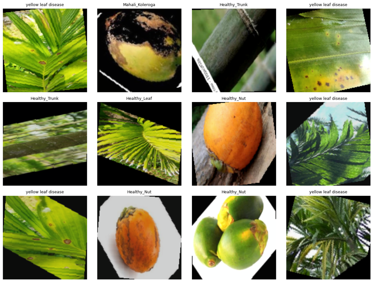
Figure 2.
Overall architecture of the proposed MSTANet. The arecanut input image is subjected to feature learning modules that include multi-scale and texture information processing. Coordinate attention is applied to the extracted features, followed by feature fusion and nine-class classification.
Figure 2.
Overall architecture of the proposed MSTANet. The arecanut input image is subjected to feature learning modules that include multi-scale and texture information processing. Coordinate attention is applied to the extracted features, followed by feature fusion and nine-class classification.
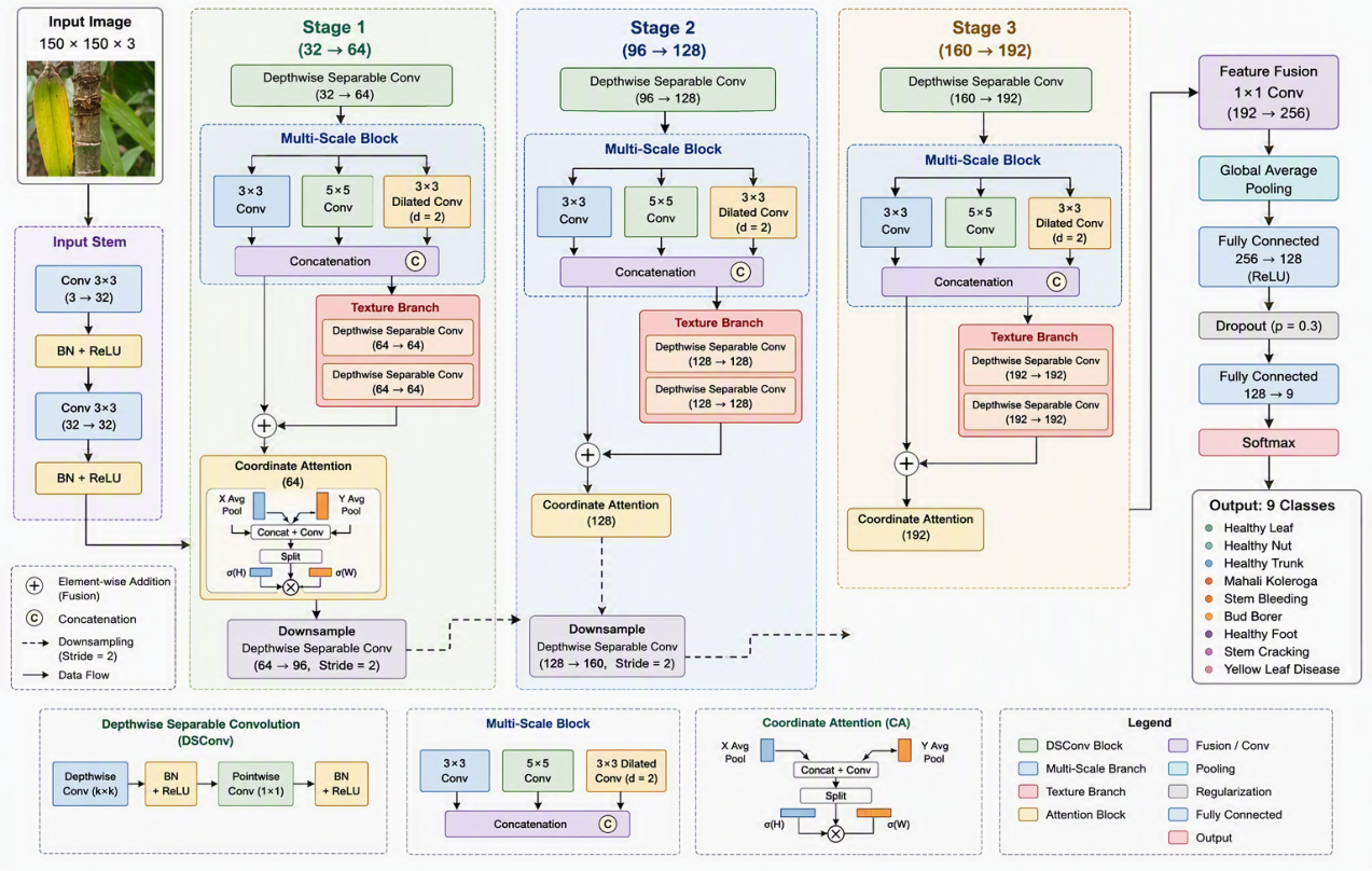
Figure 3.
Training behavior of MSTANet: (a) training and validation loss and (b) training and validation accuracy.
Figure 3.
Training behavior of MSTANet: (a) training and validation loss and (b) training and validation accuracy.
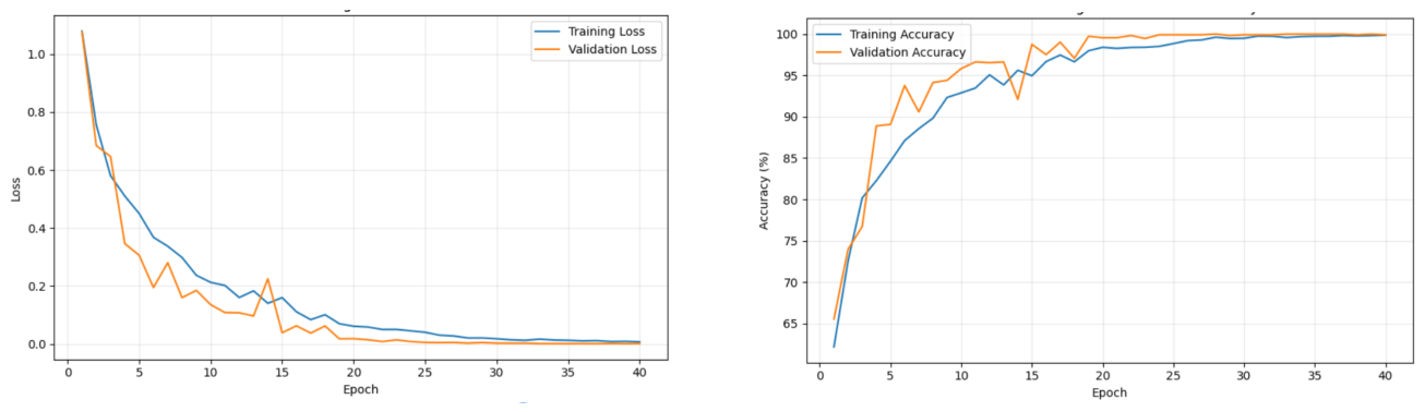
Figure 4.
MSTANet classification accuracy across the training, validation, and independent test sets.
Figure 4.
MSTANet classification accuracy across the training, validation, and independent test sets.
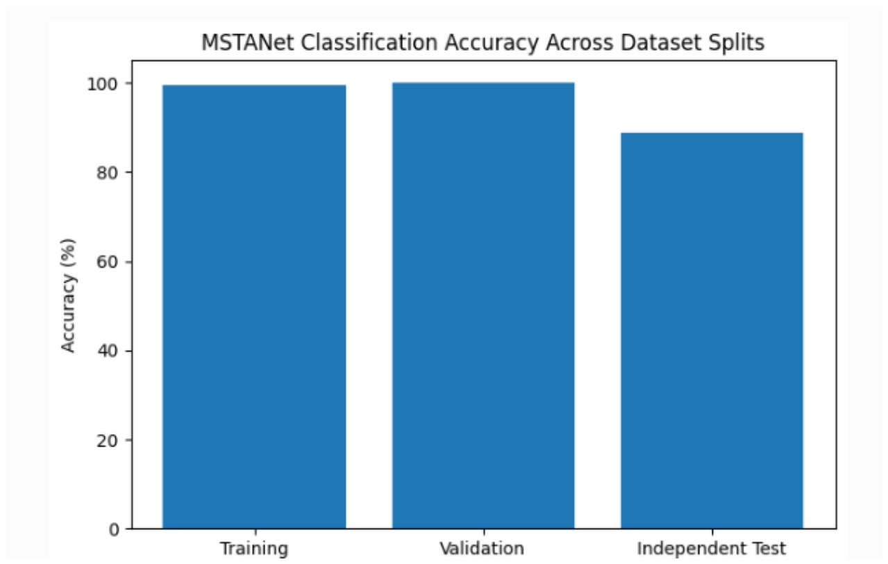
Figure 5.
Confusion matrix of MSTANet on the independent test set.
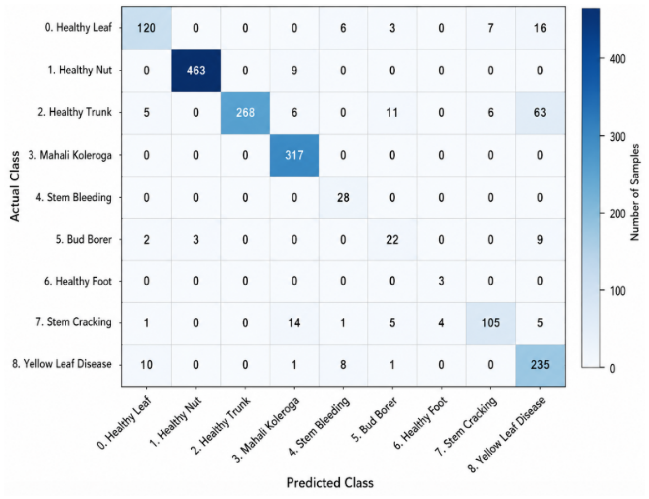
Figure 6.
Prediction confidence distribution of MSTANet for correctly and incorrectly classified samples on the independent test set. Correct predictions exhibit a substantially higher and more concentrated confidence distribution, whereas incorrect predictions show greater variability and lower confidence.
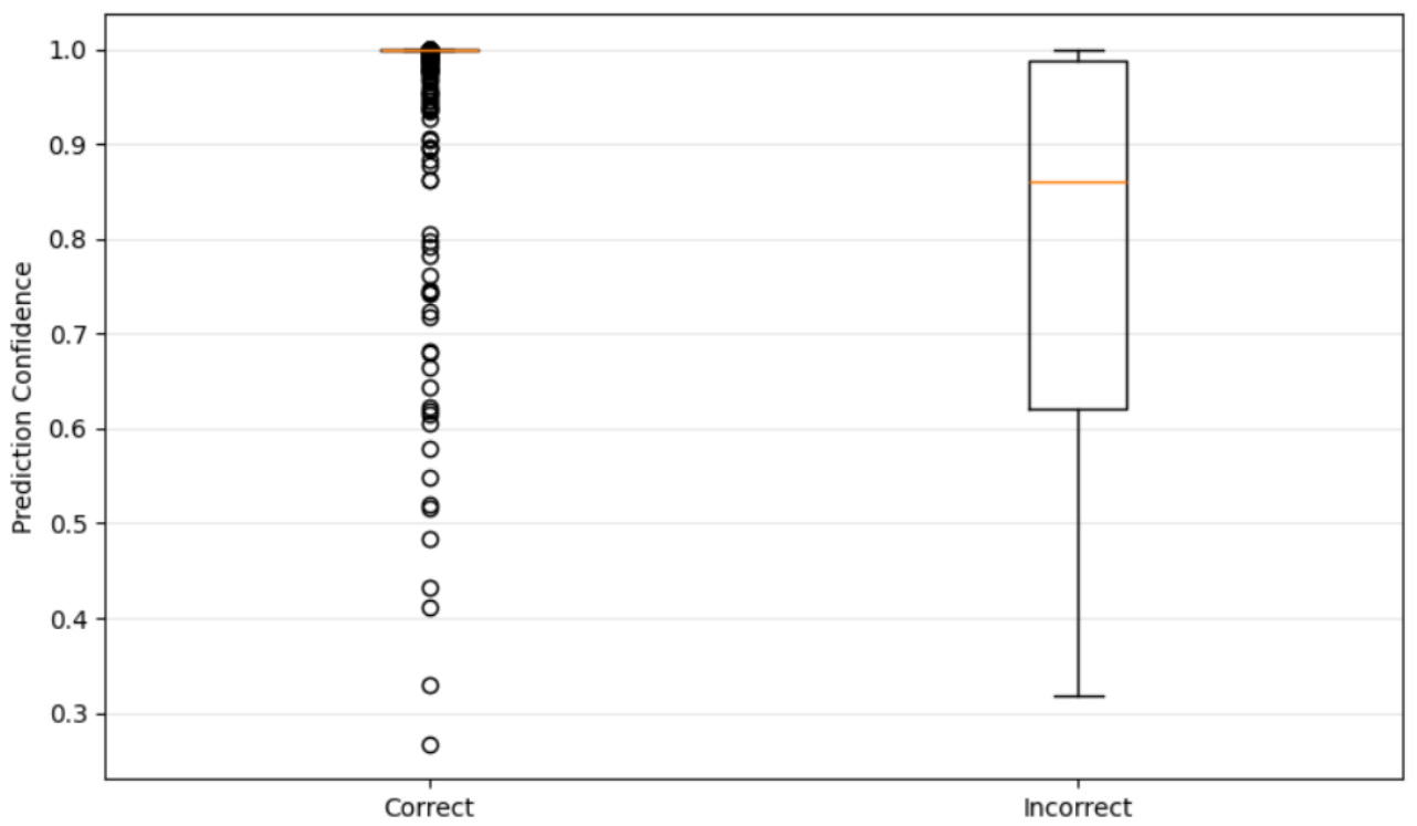
Figure 7.
Class-wise mean prediction confidence of MSTANet on the independent test set.
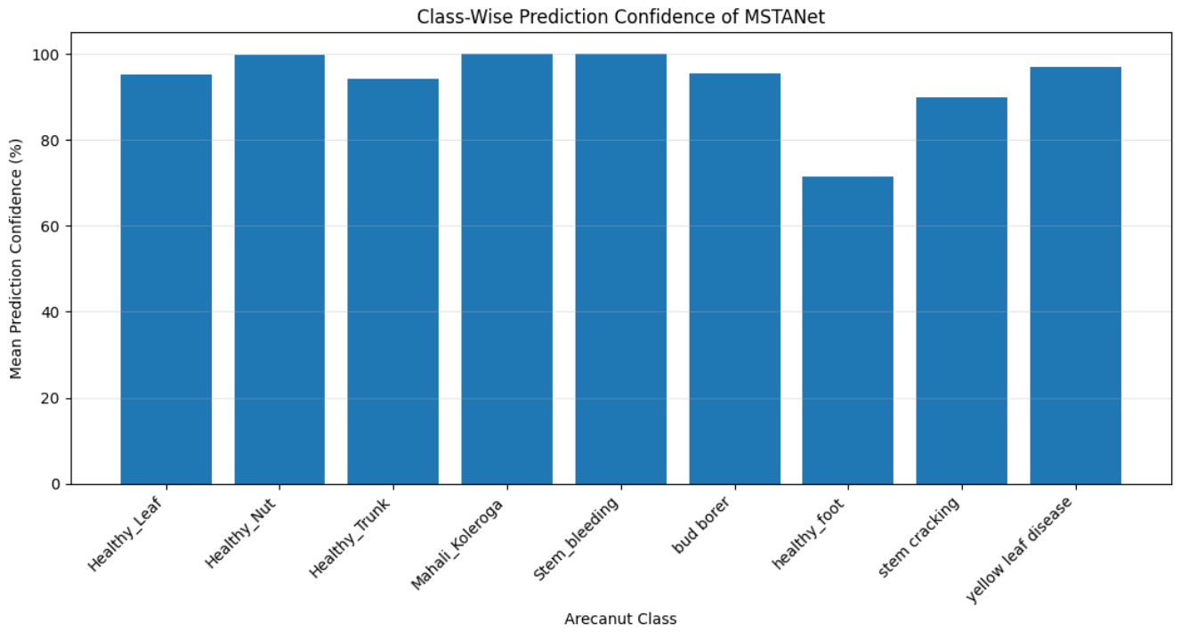

Table 1.
Dataset distribution used in the study
| Dataset Split | Number of Images |
|---|---|
| Training | 4502 |
| Validation | 1126 |
| Test | 1757 |
| Training + Validation | 5628 |
Table 2.
Training Data Augmentation Parameters
| Operation | Configuration |
|---|---|
| Image Resize | |
| Horizontal Flip | |
| Vertical Flip | |
| Random Rotation | |
| Brightness Jitter | 0.15 |
| Contrast Jitter | 0.15 |
| Saturation Jitter | 0.15 |
| Normalization | ImageNet Statistics |
Table 3.
Training Configuration of MSTANet
| Parameter | Configuration |
|---|---|
| Input Resolution | |
| Number of Classes | 9 |
| Optimizer | AdamW |
| Loss Function | Cross-Entropy Loss |
| Early Stopping | Enabled |
| Trainable Parameters | 1,397,313 |
Table 4.
Training Configuration of MSTANet
| Parameter | Configuration |
|---|---|
| Framework | PyTorch |
| Input Size | |
| Number of Classes | 9 |
| Batch Size | 32 |
| Optimizer | AdamW |
| Learning Rate | 0.001 |
| Weight Decay | 0.0001 |
| Loss Function | Cross-Entropy Loss |
| Scheduler | Cosine Annealing |
| Maximum Epochs | 40 |
| Early Stopping Patience | 7 |
| Minimum Delta | 0.001 |
| Trainable Parameters | 1,397,313 |
Table 5.
Training Summary of MSTANet
| Metric | Value |
|---|---|
| Best Epoch | 33 |
| Best Validation Accuracy (%) | 100.00 |
| Best Validation Loss | 0.0012 |
| Training Accuracy (%) | 99.58 |
| Training Loss | 0.0166 |
| Training Time (min) | 164.67 |
Table 6.
Performance Across Dataset Splits
| Dataset | Accuracy (%) | Loss |
|---|---|---|
| Training | 99.58 | 0.0166 |
| Validation | 100.00 | 0.0012 |
| Independent Test | 88.84 | – |
Table 7.
Overall Test Performance of MSTANet
| Metric | MSTANet |
|---|---|
| Accuracy (%) | 88.84 |
| Weighted Precision (%) | 90.55 |
| Weighted Recall (%) | 88.84 |
| Macro F1-score (%) | 80.15 |
| Weighted F1-score (%) | 88.97 |
| Balanced Accuracy (%) | 86.97 |
| MCC | 0.8669 |
| Cohen’s Kappa | 0.8643 |
| Weighted ROC-AUC | 0.9909 |
| Weighted PR-AUC | 0.9558 |
Table 8.
Class-Wise Classification Performance of MSTANet
| Class | Precision | Recall | F1-score | Support |
|---|---|---|---|---|
| Healthy Leaf | 0.8696 | 0.7895 | 0.8276 | 152 |
| Healthy Nut | 0.9936 | 0.9809 | 0.9872 | 472 |
| Healthy Trunk | 1.0000 | 0.7465 | 0.8549 | 359 |
| Mahali Koleroga | 0.9135 | 1.0000 | 0.9548 | 317 |
| Stem Bleeding | 0.6512 | 1.0000 | 0.7887 | 28 |
| Bud Borer | 0.5238 | 0.6111 | 0.5641 | 36 |
| Healthy Foot | 0.4286 | 1.0000 | 0.6000 | 3 |
| Stem Cracking | 0.8898 | 0.7778 | 0.8300 | 135 |
| Yellow Leaf Disease | 0.7165 | 0.9216 | 0.8062 | 255 |
| Weighted Average | 0.9055 | 0.8884 | 0.8897 | 1757 |
Table 9.
Class-Wise Prediction Confidence of MSTANet
| Class | Mean Confidence (%) |
|---|---|
| Healthy Leaf | 95.15 |
| Healthy Nut | 99.83 |
| Healthy Trunk | 94.25 |
| Mahali Koleroga | 99.97 |
| Stem Bleeding | 99.99 |
| Bud Borer | 95.51 |
| Healthy Foot | 71.39 |
| Stem Cracking | 89.86 |
| Yellow Leaf Disease | 97.04 |
Table 10.
MSTANet Model Complexity
| Property | Value |
|---|---|
| Input Resolution | |
| Output Classes | 9 |
| Trainable Parameters | 1,397,313 |
| Batch Size | 32 |
| Output Dimension | 9 |
| Training Time | 164.67 min |
Table 11.
Comparison of MSTANet with Previously Reported Nine-Class Arecanut Classification Methods
| Method | Classes | Total Images | Train Images | Test Images | Augmented Images | Test Aug. | Test Accuracy (%) |
|---|---|---|---|---|---|---|---|
| EfficientNet-B0 Dinesh (2025) | 9 | 11063 | 8847 | 1550 | NR | NR | 58.38 |
| MobileNetV3Small Dinesh (2025) | 9 | 11063 | 8847 | 1550 | NR | No | 83.87 |
| DenseNet-inspired CNN (Growth Rate = 16) Dinesh (2025) | 9 | 11063 | 8847 | 1550 | NR | NR | 87.87 |
| The proposed MSTANet | 9 | 7385 | 5628 | 1757 | Online | No | 88.84 |
Disclaimer/Publisher’s Note: The statements, opinions and data contained in all publications are solely those of the individual author(s) and contributor(s) and not of MDPI and/or the editor(s). MDPI and/or the editor(s) disclaim responsibility for any injury to people or property resulting from any ideas, methods, instructions or products referred to in the content. |
© 2026 by the authors. Licensee MDPI, Basel, Switzerland. This article is an open access article distributed under the terms and conditions of the Creative Commons Attribution (CC BY) license (http://creativecommons.org/licenses/by/4.0/).
Copyright: This open access article is published under a Creative Commons CC BY 4.0 license, which permit the free download, distribution, and reuse, provided that the author and preprint are cited in any reuse.