

Submitted:
29 September 2026
Posted:
29 September 2026
You are already at the latest version
Abstract
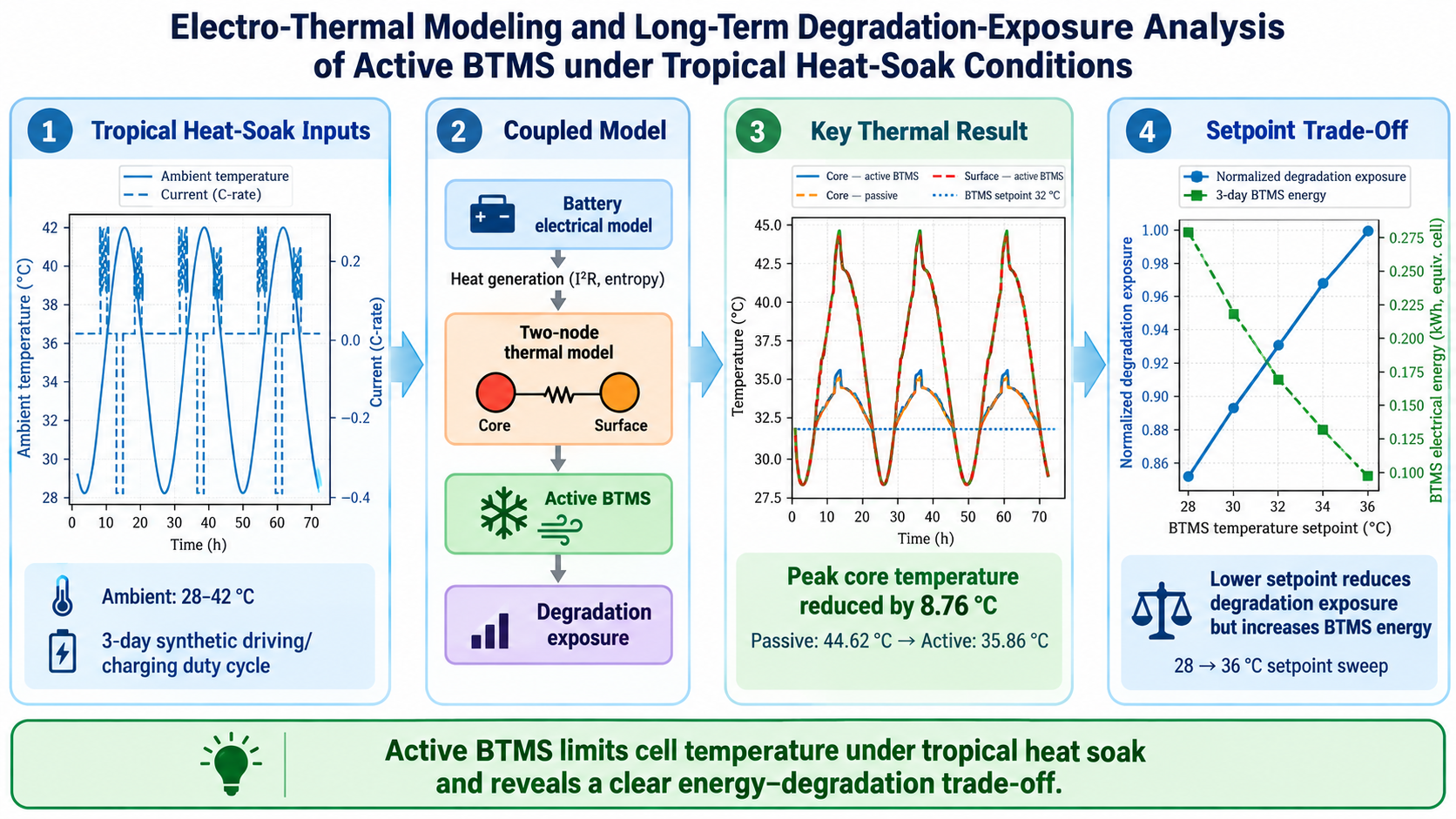
High ambient temperature and repeated heat-soak exposure can increase the thermal-management burden of electric-vehicle batteries and accelerate temperature-sensitive degradation mechanisms. This study develops a coupled simulation framework combining a second-order resistor–capacitor equivalent-circuit model, state-of-charge dynamics, Bernardi-type heat generation, a two-node core–surface thermal network, proportional active battery thermal management, and Arrhenius-weighted degradation exposure. A repeatable tropical boundary condition of 28–42 \( ^{\circ}C \) is imposed together with a synthetic driving/charging duty cycle. Under the reference parameter set, active thermal management limits the peak simulated core temperature to 35.86 \( ^{\circ}C \) compared with 44.62 \( ^{\circ}C \) for passive operation, a reduction of 8.76 \( ^{\circ}C \). The three-day equivalent-cell BTMS electrical demand is 0.166 kWh and the integrated heat removal is 0.243 kWh. Active cooling reduces the normalized cumulative degradation exposure by approximately 14.0% relative to passive operation. Setpoint sweeps from 28 to 36 \( ^{\circ}C \) quantify the trade-off between cooling energy and degradation exposure. Because cell-specific aging data are not yet available, long-term results are reported as normalized degradation exposure rather than experimentally validated percentage SoH. The framework therefore provides a reproducible basis for subsequent parameter identification, experimental validation, and pack-level lifetime optimization under tropical operating conditions.
Keywords:
battery thermal management system
; electro-thermal model
; lithium-ion battery
; 2RC equivalent circuit
; tropical heat soak
; state of health
; degradation
; electric vehicle
1. Introduction
From an industrial and systems-engineering perspective, battery thermal management can also be viewed as an operational decision problem rather than only a component-level thermal design problem. In electric-vehicle applications, the selected thermal-management strategy influences not only battery temperature but also auxiliary energy consumption, degradation-related exposure, operating reliability, and long-term system cost. Therefore, a model that links electrical loading, heat generation, cooling-energy demand, and degradation-related stress can support engineering decisions on operating policy, resource utilization, and lifecycle performance of battery systems under severe environmental conditions. Lithium-ion batteries (LIBs) have become the dominant electrochemical energy-storage technology for battery electric vehicles and plug-in hybrid electric vehicles because they combine high specific energy, high power capability, low self-discharge, and comparatively long service life. Their practical performance, however, is strongly temperature dependent. Cell temperature affects ionic transport, charge-transfer kinetics, internal resistance, usable capacity, power capability, charging acceptance, heat generation, and degradation rate. Consequently, thermal management is not an auxiliary consideration but an integral part of the electrical, energy-management, and lifetime design of an electric-vehicle battery system [1,2,3,24]. At pack level, these effects become more complex because individual cells experience different thermal boundary conditions and electrical loads, while the energy required by pumps, fans, compressors, or chillers is drawn from the vehicle energy budget. An effective battery thermal management system (BTMS) must therefore control battery temperature without introducing an excessive parasitic-energy penalty.
Temperature is also closely coupled to battery durability. Elevated temperature generally accelerates parasitic electrochemical reactions, solid-electrolyte-interphase growth, electrolyte decomposition, active-material degradation, and resistance evolution. Conversely, low-temperature operation can restrict charge transfer and diffusion and can increase the risk of lithium plating during charging. Both calendar and cycling degradation therefore depend on combinations of temperature, state of charge (SoC), depth of discharge, current rate, accumulated throughput, and elapsed time [4,5,6,7,14]. Reviews of BTMS design consequently emphasize operation within a moderate thermal range and minimization of large temperature gradients, although the exact preferred range depends on cell chemistry, operating duty, and manufacturer constraints [1,3]. These considerations are particularly important for high-power operation and fast charging, where electrical losses and electrochemical polarization can increase heat-generation rates over relatively short periods.
The thermal problem becomes more demanding when electric vehicles are operated in persistently hot environments. Unlike a short high-current event, tropical or hot-climate operation can expose the battery to elevated ambient temperature for many hours, including periods when the vehicle is parked and electrical load is small. During such heat-soak periods, the surrounding environment can continue to raise or maintain battery temperature, thereby reducing the opportunity for the battery to return to a lower thermal baseline before the next driving or charging event. Shojaei et al. demonstrated the importance of this issue for plug-in hybrid vehicles in hot climates and showed that battery cooling during parked conditions introduces a non-trivial compromise between battery lifetime and auxiliary-energy demand [21]. More generally, vehicle-level studies have demonstrated that driving cycle, ambient temperature, charging mode, and trip duration alter the thermal and aging histories experienced by an EV battery [22]. These findings indicate that battery temperature should be evaluated as a time-dependent state driven jointly by electrical loading and environmental exposure rather than as a fixed boundary condition.
Recent BTMS research has addressed this problem through air cooling, indirect and direct liquid cooling, immersion cooling, phase-change materials, heat pipes, and hybrid configurations [1,3,24]. The selection of a cooling architecture involves competing requirements. Increasing coolant flow rate, reducing coolant inlet temperature, or activating refrigeration more aggressively can lower battery temperature, but the resulting pressure drop, pumping requirement, compressor load, mass, cost, and control complexity can reduce system-level efficiency. Recent WEVJ studies illustrate the continuing development of this field. Onreabroy and Kaewpradap investigated an optimized air-cooling strategy under different discharge rates, inlet-air temperatures, and flow conditions, demonstrating the strong coupling between operating conditions and achievable battery temperature [26]. More recently, Larra naga-Ezeiza et al. experimentally compared partial direct liquid cooling with conventional indirect liquid cooling and showed that thermal-management architecture can materially affect measured degradation and internal-resistance evolution under equivalent electro-thermal stress [27]. These results reinforce an important point: BTMS performance should ultimately be evaluated not only by instantaneous temperature reduction but also by its implications for battery degradation and the energy required to achieve that reduction.
A second challenge concerns the model used to connect electrical operation, heat generation, battery temperature, and thermal-management demand. Detailed electrochemical and computational-fluid-dynamics models can provide high physical fidelity, but their parameter requirements and computational cost may limit their use in repeated control, sensitivity, lifetime, and optimization studies. Reduced-order electro-thermal models therefore remain attractive for battery-management and vehicle-level applications. Equivalent-circuit models (ECMs), in particular, provide an effective compromise between dynamic fidelity and computational efficiency. A second-order resistor–capacitor ECM (2RC-ECM) represents the instantaneous ohmic voltage drop together with two polarization dynamics occurring at different characteristic time scales [8,9]. Karimi et al. showed that operating temperature, SoC, and current rate significantly influence ECM parameter accuracy, highlighting the need for operating-condition-dependent parameterization [8]. Similarly, experimentally characterized second-order ECMs have been used as the electrical foundation of battery thermal-management studies [16].
The electrical model alone is insufficient because its parameters and losses depend on temperature, while those losses simultaneously generate heat. A physically consistent electro-thermal model must therefore establish a closed coupling between the electrical and thermal domains. Huang et al. combined a second-order RC electrical model with a two-state lumped thermal network and demonstrated the usefulness of representing both electrical dynamics and internal thermal behavior within a unified reduced-order structure [10]. Naguib et al. likewise developed a coupled 2RC electro-thermal model with experimentally identified parameters and validated its response under multiple dynamic operating conditions [9]. Reduced-order approaches are also relevant to real-time battery-management applications. Li et al. demonstrated that an electro-thermal battery representation can be reduced sufficiently for software-in-the-loop and hardware-in-the-loop BMS assessment while retaining the principal electrical and thermal dynamics [23]. More recent layered electro-thermal equivalent-circuit approaches have further emphasized the value of distinguishing internal and surface temperatures instead of treating the entire cell as a single isothermal body [11].
Within such a coupled model, heat generation must be evaluated consistently with the electrical states. The general battery energy balance introduced by Bernardi, Pawlikowski, and Newman provides a widely used basis for separating irreversible and reversible heat-generation components [12]. The irreversible contribution reflects ohmic and polarization losses, whereas reversible heat is associated with the entropy coefficient, commonly represented through . This distinction is relevant because using an independently prescribed heat source can break the physical link between terminal-voltage loss and thermal response. Conversely, including a reversible-heat function without chemistry-specific entropy data introduces another unsupported assumption. For this reason, a transparent reduced-order model should either use experimentally available entropy-coefficient data or explicitly identify the omission of the reversible contribution as a modeling limitation.
A third issue is the connection between short-term thermal behavior and long-term battery health. Calendar-aging models commonly incorporate temperature and SoC dependence, while cycling-aging formulations additionally consider factors such as charge throughput, C-rate, and depth of discharge [4,5,13]. Arrhenius-type temperature acceleration is widely employed because many degradation mechanisms are strongly thermally activated. However, the fitted coefficients remain chemistry- and experiment-dependent. Consequently, an aging equation calibrated for one cell chemistry, format, or operating window cannot automatically provide quantitative SoH predictions for another battery. Reviews of battery degradation models consistently identify model calibration, operating-condition coverage, and transferability as major limitations in lifetime prediction [4,14]. This distinction is essential when electro-thermal simulations are extended over months or years: a model can compare relative degradation stress among operating strategies without necessarily supporting an absolute claim such as a specific percentage of remaining SoH.
This issue is increasingly relevant as BTMS research shifts from temperature minimization toward health- and energy-aware control. Battery cooling consumes electrical energy and therefore competes directly with traction range and overall vehicle efficiency. Shojaei et al. demonstrated this trade-off for hot-climate cooling by considering battery lifetime together with vehicle-level energy consequences [21]. Nam and Ahn subsequently developed an ANN-assisted model-predictive BTMS controller and demonstrated that thermal constraints and auxiliary-energy consumption can be treated simultaneously rather than independently [25]. Similar system-level studies have incorporated battery degradation into vehicle energy and thermal-management objectives [17]. Collectively, these studies indicate that neither minimum temperature nor minimum BTMS energy is sufficient as an isolated design objective. The more relevant engineering question concerns how much thermal and degradation benefit is obtained for the additional cooling energy supplied by the vehicle.
Despite these advances, several gaps remain when the objective is to evaluate active BTMS operation under sustained tropical heat-soak conditions. First, many thermal-management studies concentrate on cooling architecture, channel geometry, airflow configuration, or instantaneous maximum temperature, whereas fewer studies follow a computationally inexpensive but physically coupled chain from dynamic electrical loading to heat generation, internal temperature, cooling energy, and degradation stress. Second, electro-thermal modeling studies commonly emphasize parameter estimation and short-duration voltage/temperature validation but do not necessarily examine the repeated hot-soak exposure encountered in tropical environments. Third, lifetime-oriented models can predict capacity fade when a chemistry-specific aging dataset is available, but applying such models without calibration risks introducing apparently precise but unsupported SoH values. Finally, sensitivity and optimization studies sometimes evaluate BTMS operating points separately from the model used to generate the principal thermal results. A more transparent approach is to generate every ambient-temperature and cooling-setpoint condition by rerunning the same coupled electro-thermal framework.
The importance of temporally resolved battery loading is also consistent with previous work on electric-vehicle charging and grid interaction. Studies by Yosrueangsak et al. and Chitgreeyan et al., involving members of the present research group, examined vehicle-to-grid operation and multi-period EV charging control, respectively [19,20]. Although those studies addressed grid-level rather than cell-level electro-thermal phenomena, they reinforce the broader requirement that EV power demand and charging should be represented as time-dependent operating conditions. In the present work, this principle is transferred to the battery level through a repeatable driving/charging duty cycle, allowing thermal-management alternatives to be compared under identical temporal excitation.
Accordingly, this study develops a unified reduced-order framework for investigating active BTMS behavior under tropical heat-soak conditions. A temperature- and SoC-dependent 2RC-ECM is coupled to Bernardi-type heat generation and a two-node core–surface thermal network. The active BTMS is represented through controlled heat removal, while thermal cooling capacity and BTMS electrical power are treated as distinct physical quantities. The numerical boundary condition spans a repeated tropical ambient-temperature cycle of 28–42 °C together with a time-varying driving/charging profile. Active and passive thermal-management cases are compared using the same electro-thermal chain, after which the complete model is rerun over different ambient-temperature shifts and BTMS setpoints. Long-term thermal influence is evaluated through Arrhenius-weighted calendar- and cycling-degradation exposure rather than through an uncalibrated absolute SoH prediction.
In addition, the framework provides an industrial-engineering-oriented basis for evaluating the trade-off between thermal protection, auxiliary-energy consumption, and degradation-related exposure. This enables the BTMS setpoint and cooling strategy to be interpreted as operational decision variables that affect system efficiency, reliability, and lifecycle performance. The principal contribution is therefore not a new cooling-hardware geometry, nor is it a claim of experimentally validated lifetime prediction. Instead, the work provides a numerically consistent bridge among four quantities that are frequently treated separately: electrical operating state, internal battery temperature, BTMS energy demand, and degradation-related thermal exposure. Specifically, the study (i) couples a true second-order ECM with dynamic polarization states to a two-node core–surface thermal network; (ii) derives the thermal source from the same electrical states used in the transient solution; (iii) separates heat removed by the BTMS from the electrical energy required to provide that cooling; (iv) evaluates degradation through a relative, explicitly uncalibrated stress formulation so that unsupported quantitative SoH claims are avoided; and (v) constructs ambient-temperature and setpoint trade-off curves exclusively from complete model reruns rather than manually assigned performance points. This formulation is intended to provide a reproducible baseline for the active-versus-passive, tropical-temperature, and BTMS-setpoint comparisons reported in the following sections and, subsequently, for cell-specific HPPC, thermal-transient, and aging-model calibration.
2. Materials and Methods
2.1. Overall Coupled Framework
Figure 1 presents the overall structure of the proposed coupled electro–thermal–BTMS framework developed for evaluating battery behavior under repeated tropical heat-soak conditions. The model is organized as a sequence of interacting electrical, thermal, cooling, and degradation-related subsystems rather than as independent calculation blocks. This arrangement reflects the physical coupling that exists in lithium-ion batteries: electrical loading produces internal losses and heat generation, the resulting temperature affects the electrical characteristics of the cell, and the accumulated temperature and operating history subsequently influence both the cooling requirement and degradation-related stress [2,9,16].
The framework begins with two time-dependent boundary conditions, namely the ambient temperature and battery current . The ambient-temperature profile represents repeated exposure to a tropical environment, whereas the current profile represents the electrical demand associated with driving, charging, and low-load periods. These two inputs are applied consistently throughout the simulation so that active and passive thermal-management strategies can be compared under identical operating conditions. In this study, the use of a repeatable duty cycle is intended to isolate the influence of thermal management and ambient temperature from variations in the electrical loading history.
The electrical response of the battery is represented by a second-order resistor–capacitor equivalent-circuit model (2RC-ECM). The model calculates the state of charge (SoC), terminal voltage , and the two polarization-voltage states and . The corresponding resistive and polarization elements, , , , , and , provide a reduced-order representation of the principal dynamic electrical processes occurring during charge and discharge. A 2RC structure is adopted because it provides a suitable compromise between model fidelity and computational efficiency for repeated simulation, sensitivity analysis, and control-oriented battery studies [8,9]. In the present framework, the electrical parameters can vary with SoC and temperature, thereby establishing feedback between the electrical and thermal domains.
The heat-generation block provides the physical connection between the electrical and thermal models. Electrical losses calculated from the ECM are converted into the heat-generation rate , which acts as the thermal source for the battery cell. This treatment avoids prescribing an independent heat-input profile and instead ensures that the thermal excitation is linked directly to the electrical operating state. The formulation follows the general energy-balance concept commonly used for lithium-ion batteries, in which irreversible electrical losses and, when appropriate data are available, reversible entropic heat can be considered [12].
The generated heat is subsequently introduced into a two-node thermal network representing the cell core temperature and surface temperature . The thermal resistances and describe heat transfer from the cell core to the surface and from the surface to the ambient environment, respectively, while and represent the corresponding thermal capacitances. Separating the core and surface nodes provides a more physically meaningful description of transient battery temperature than a single lumped-temperature state while retaining considerably lower computational cost than a detailed three-dimensional thermal model [10,11]. The resulting core–surface temperature difference is therefore obtained from the thermal dynamics rather than imposed through an empirical temperature offset.
The active BTMS interacts directly with the surface thermal node. When the surface temperature exceeds the prescribed control threshold, the controller determines the required cooling rate . This heat-removal term modifies the surface energy balance and consequently affects both surface and core temperatures. In addition to the thermal cooling rate, the framework separately evaluates the electrical power required by the BTMS, denoted by . This distinction is necessary because the amount of heat removed from the battery and the electrical energy consumed by the cooling system represent different physical quantities. Consequently, the framework can evaluate not only the thermal benefit of active cooling but also the corresponding auxiliary-energy penalty.
The electrical and thermal states are also used to evaluate degradation-related exposure. The calendar-aging component is associated primarily with temperature and SoC history, whereas the cycling component additionally reflects the applied current or C-rate. Arrhenius-type temperature dependence is used to represent the acceleration of degradation processes with increasing temperature, consistent with widely used semi-empirical battery-aging approaches [4,5,13]. However, because cell-specific aging coefficients have not yet been identified from long-duration experimental data, the present study reports a normalized degradation-exposure index rather than absolute capacity loss or percentage SoH. This treatment allows relative comparisons among operating strategies without introducing unsupported quantitative lifetime predictions.
The outputs of the individual model components are finally combined to evaluate battery temperature, BTMS energy demand, and degradation-related exposure. These quantities provide the basis for comparing active and passive thermal-management cases and for examining the sensitivity of the system to ambient temperature and BTMS setpoint. Importantly, all subsequent numerical results are generated from the same coupled simulation chain. Thus, changes in thermal response, cooling-energy requirement, and degradation exposure remain internally consistent with the imposed electrical and environmental conditions.
Figure 1 therefore represents the central computational concept of the study. The upper pathway describes the progression from environmental and electrical excitation to heat generation and battery temperature, whereas the lower pathway extends the thermal response to active cooling, degradation exposure, and system-level performance assessment. This unified structure provides a reproducible basis for the subsequent analyses while also allowing future experimental parameter identification and aging calibration to be incorporated without changing the fundamental organization of the model.
2.2. Reference Cell and Boundary Conditions
The present numerical study uses a 50 Ah equivalent cell representation and a repeatable three-day duty cycle with a 10 s integration step. The ambient-temperature profile is sinusoidal between 28 and 42 °C. Positive current denotes discharge and negative current denotes charge. The synthetic schedule contains morning and evening driving intervals and a midday charging interval. The profile is intentionally deterministic to enable direct comparisons across cooling setpoints and ambient-temperature shifts. It should not be interpreted as a measured WLTP, UDDS, or field driving cycle.
Table 1 lists the reference parameters used in the present numerical model. These values are an internally consistent reference set for framework testing; they are not claimed to be identified parameters of a specific commercial cell. Before experimental publication, and the 2RC parameters should be identified from cell-level pulse/HPPC tests over the intended SoC–temperature operating region, as commonly performed in electro-thermal ECM studies [8,16].
2.3. Second-Order Equivalent-Circuit Model
The dynamic electrical behavior of the equivalent battery cell is represented by a second-order resistor–capacitor equivalent-circuit model (2RC-ECM). This model is selected because it provides a practical compromise between computational efficiency and the ability to reproduce the transient voltage response of lithium-ion cells over different operating conditions. Compared with a simple internal-resistance or first-order RC model, the additional polarization branch allows the model to represent two characteristic relaxation time scales while remaining sufficiently compact for repeated electro–thermal simulations and sensitivity analyses [8,9,18].
The model consists of an open-circuit-voltage source, an instantaneous ohmic resistance , and two parallel RC polarization branches characterized by and . The ohmic resistance primarily accounts for the instantaneous voltage drop associated with current flow, whereas the two RC branches reproduce the slower dynamic voltage response that develops during charge and discharge. The two branches should be interpreted as reduced-order representations of battery polarization dynamics rather than as unique representations of individual electrochemical mechanisms. Their different time constants, and , allow the ECM to describe both relatively fast and relatively slow relaxation behavior.
With discharge current defined as positive, the polarization-voltage states are
where and are the dynamic voltage drops associated with the first and second polarization branches, respectively. Under a change in current, these states do not respond instantaneously but evolve according to their corresponding RC time constants. This dynamic behavior is particularly relevant to the present study because the applied duty cycle contains repeated transitions among discharge, charging, and zero-current periods.
The terminal voltage is calculated from
Here, represents the equilibrium open-circuit voltage, which may depend on both state of charge and temperature. The term represents the instantaneous ohmic voltage loss, while and account for the dynamic polarization contributions. Equation (3) therefore provides the connection between the imposed current profile and the electrical losses that subsequently contribute to battery heat generation.
The state of charge is propagated using Coulomb counting,
where is the nominal cell capacity in ampere-hours. Under the adopted sign convention, positive current reduces SoC during discharge, whereas negative current increases SoC during charging. The calculated SoC is subsequently used not only in the electrical model but also as an operating variable in the degradation-exposure analysis.
The electrical and thermal models are coupled through the temperature dependence of the ECM parameters. In the present reference implementation, the resistance parameters are modified by smooth SoC- and temperature-dependent scaling relationships. As the cell temperature changes, the corresponding resistance values and electrical losses are therefore updated, which in turn changes the heat-generation rate supplied to the thermal model. This feedback creates the electro–thermal interaction illustrated in Figure 1. The temperature- and SoC-dependent behavior of the reference ohmic resistance is subsequently examined in Figure 3.
For the present numerical investigation, the reference ECM parameters listed in Table 1 are used consistently across the baseline and sensitivity simulations. They provide an internally consistent parameter set for assessing the behavior of the proposed coupled framework but are not presented as experimentally identified parameters of a specific commercial cell. For cell-specific implementation, and the parameter surfaces , , , , and should be obtained from pulse or hybrid pulse power characterization tests performed over the relevant temperature and SoC ranges [8,9,16]. Such characterization would also permit independent validation of the simulated terminal-voltage response before the model is used for quantitative thermal and lifetime prediction.
2.4. Heat-Generation Model
The thermal source used in the coupled model is derived directly from the electrical response of the battery rather than prescribed independently. This treatment maintains consistency between the electrical losses predicted by the 2RC-ECM and the heat subsequently transferred to the thermal model. The total heat-generation rate is formulated using the general energy-balance concept proposed by Bernardi et al. [12]. In the present ECM implementation,
where is the total heat-generation rate, I is the battery current, is the open-circuit voltage, is the terminal voltage obtained from the 2RC-ECM, and T is the absolute cell temperature.
The first term, , represents irreversible heat generation associated with the difference between the equilibrium cell voltage and the operating terminal voltage. In the present framework, this voltage difference includes the instantaneous ohmic loss through together with the dynamic polarization contributions represented by and . Consequently, the irreversible heat-generation term is directly linked to the electrical states described by Equations (1)–(3). An increase in current or internal electrical loss therefore produces a corresponding increase in the thermal source supplied to the cell model.
The second term, , represents reversible entropic heat associated with the temperature dependence of the electrochemical equilibrium potential. Unlike irreversible heating, the reversible contribution can act either as a heat source or a heat sink depending on the sign of the entropy coefficient, operating current direction, and state of charge. Reliable evaluation of this term therefore requires a chemistry-specific relationship between and SoC.
In the present numerical study, such entropy-coefficient data are not available for the reference cell. The reversible contribution is therefore set to zero in the baseline simulations rather than introducing an assumed or empirically constructed relationship. This treatment limits the thermal source to the irreversible heat predicted from the electrical model and avoids attributing unsupported reversible heating or cooling to the simulated cell.
The resulting is applied directly to the core node of the two-node thermal network described in the following subsection. This provides the principal electrical-to-thermal coupling within the proposed framework: the applied current and electrical states determine the heat-generation rate, whereas the resulting cell temperature subsequently influences the temperature-dependent ECM parameters. The transient heat-generation behavior obtained from this formulation is evaluated later in Figure 4.
For a cell-specific implementation, the entropy coefficient should be experimentally characterized over the relevant SoC and temperature ranges or obtained from independently validated data for the same chemistry. Incorporating such information would allow both irreversible and reversible heat-generation mechanisms to be represented without altering the overall structure of the coupled electro–thermal model.
2.5. Two-Node Core–Surface Thermal Model
The thermal response of the equivalent cell is represented using a two-state lumped thermal network that distinguishes the internal core temperature, , from the external surface temperature, . This reduced-order structure provides greater physical meaning than a single-temperature model because heat is generated primarily within the cell and must subsequently propagate toward the surface before being rejected to the surrounding environment or removed by the BTMS. At the same time, the model remains sufficiently compact for repeated electro–thermal simulations, controller evaluation, and sensitivity studies [10,11].
The core and surface nodes are characterized by the thermal capacitances and , respectively. These parameters represent the ability of each region to store thermal energy. Heat transfer between the two nodes is governed by the effective core–surface thermal resistance , whereas heat rejection from the surface to the surrounding environment is represented by the surface–ambient thermal resistance . The resulting network therefore captures the principal thermal pathway from internal heat generation to the external cooling boundary without requiring a detailed spatial thermal model.
The core energy balance is
where is the heat-generation rate obtained from the electrical model. The first term on the right-hand side represents thermal energy generated within the cell, whereas the second term represents heat conducted from the core toward the surface. When , heat is transferred outward through , causing the core temperature to decrease relative to the case in which no internal heat-transfer path is considered.
The surface energy balance is
The first term on the right-hand side represents heat arriving from the core. The second term describes passive heat exchange between the cell surface and the ambient environment, while the final term represents active heat removal by the BTMS. Consequently, the surface node acts as the interface between the internal battery thermal dynamics and the external thermal-management system.
The two-node formulation is especially relevant under transient loading because the core and surface do not necessarily respond at the same rate. During periods of increased electrical loading, heat generated internally can cause the core temperature to rise before the full thermal response appears at the surface. Conversely, when the external cooling system is activated, the surface can respond more rapidly than the core. This behavior produces a finite core–surface temperature difference that reflects the thermal inertia of the cell.
In the present framework, the quantity is therefore interpreted as an internal thermal-gradient indicator generated directly by the energy-balance equations. It is not imposed through an empirical correction or C-rate-dependent offset. This distinction is important because the resulting temperature difference remains physically connected to the modeled heat generation, thermal capacitances, thermal resistances, ambient temperature, and BTMS cooling action.
The model should nevertheless be interpreted within its reduced-order resolution. The quantity does not represent complete module-scale temperature uniformity because the present framework contains only one equivalent cell with two thermal states. Cell-to-cell variation, coolant-channel maldistribution, contact resistance, and localized hotspots are not explicitly resolved. Such effects would require a multi-cell thermal network, distributed temperature measurements, or a higher-dimensional numerical model.
The calculated surface temperature is subsequently used as the feedback variable for the active BTMS controller described in the following subsection. In this way, Equations (6) and (7) provide the central thermal link between the electrically generated heat and the controlled cooling rate within the overall coupled framework.
2.6. Active BTMS Controller and Electrical Overhead
The active battery thermal management system is represented as a feedback-controlled heat-removal mechanism acting on the surface node of the two-node thermal model. The surface temperature is selected as the controller input because it is the thermal state directly coupled to the external cooling system in the reduced-order framework. This choice also provides a clear connection between the thermal model described in Equations (6) and (7) and the cooling action imposed by the BTMS.
The commanded heat-removal rate is expressed as
where is the prescribed BTMS temperature setpoint, is the proportional control gain, and is the maximum available cooling capacity. When , the term becomes zero and no active cooling is requested. Once the surface temperature exceeds the setpoint, the commanded cooling rate increases in proportion to the temperature difference .
The min operator limits the cooling command to and therefore represents the finite thermal capacity of the cooling system. This saturation is important because a practical BTMS cannot increase heat removal indefinitely as battery temperature rises. Under mild thermal conditions, the proportional controller can regulate the cooling demand according to the surface-temperature deviation. Under more severe heat-soak or electrical-loading conditions, the controller may reach its maximum cooling capacity, after which any additional thermal load must be absorbed by the battery thermal mass or rejected through the passive surface–ambient pathway.
The present proportional controller is intentionally simple. Its purpose is not to reproduce the detailed supervisory control logic of a commercial electric vehicle but to provide a transparent and repeatable control law for evaluating the influence of the BTMS setpoint on battery temperature and cooling demand. This formulation is particularly suitable for the present sensitivity analysis because the same controller structure is retained while is varied systematically. Consequently, differences among the setpoint cases arise from the thermal response of the coupled model rather than from changes in controller architecture.
An important feature of the proposed framework is that the thermal heat-removal rate and the electrical power required to operate the BTMS are treated as separate quantities. The quantity represents heat removed from the battery and enters directly into the surface energy balance in Equation (7). It is therefore a thermal quantity and should not be interpreted as electrical power consumption.
When cooling is active, the corresponding BTMS electrical demand is estimated from
and when cooling is inactive. Here, denotes the reference coefficient of performance of the cooling system and represents the auxiliary electrical demand of the coolant circulation system.
Equation (9) provides a simplified system-level estimate of the electrical energy required to deliver a given thermal cooling rate. The term represents the electrical demand associated with the active cooling process, while accounts for the additional circulation power required whenever the BTMS is operating. This separation allows the model to distinguish between the thermal benefit obtained by removing heat from the battery and th
2.7. Degradation-Exposure Model
The degradation component of the proposed framework is used to evaluate how the electrical and thermal operating histories influence the relative aging stress experienced by the battery. Lithium-ion battery degradation is commonly separated into calendar and cycling contributions because the two mechanisms are associated with different operating conditions and stress factors. Calendar aging occurs continuously with elapsed time and is strongly influenced by temperature and state of charge, whereas cycling aging is additionally affected by charge/discharge current, C-rate, depth of discharge, and accumulated charge throughput [4,5,6].
Temperature is particularly important because many degradation mechanisms are thermally activated. Elevated temperature can accelerate side reactions, interfacial-film growth, electrolyte decomposition, and other processes that contribute to capacity loss and resistance increase. Arrhenius-type relationships are therefore widely employed in semi-empirical battery-aging models to represent the temperature dependence of degradation rates [4,5,13]. In the present framework, these relationships are used to construct relative degradation-stress rates rather than to predict absolute capacity loss.
The calendar-aging stress factor is expressed as
where denotes the relative calendar-aging stress rate, is the corresponding activation energy, R is the universal gas constant, T is the instantaneous cell temperature in Kelvin, and is the reference temperature. The function represents the influence of state of charge on calendar-aging stress.
The temperature term in Equation (10) increases the relative stress as the cell temperature rises above the reference condition. The SoC-dependent term accounts for the additional influence of storage or operation at different charge levels. Consequently, the calendar-stress contribution can accumulate even when the applied current is zero. This feature is particularly relevant to tropical heat-soak operation, where the battery may remain exposed to elevated temperature during parked or low-load periods.
The cycling-related stress factor is represented as
where is the relative cycling-stress rate, C denotes the instantaneous C-rate, is the activation energy associated with the cycling-related temperature dependence, and represents the sensitivity of the cycling stress to current rate. The absolute value of C is used because both charging and discharging contribute to battery usage, although their detailed degradation effects can differ in a fully calibrated aging model.
Equation (11) therefore combines two principal effects. The C-rate term increases the relative stress during periods of higher electrical loading, whereas the Arrhenius term amplifies this stress when cycling occurs at elevated temperature. In the present operating profile, cycling-related stress is consequently concentrated primarily during the driving and charging intervals, whereas the calendar contribution continues to accumulate throughout the complete thermal history.
The instantaneous calendar and cycling stress rates are evaluated using the temperature, SoC, and current histories obtained from the coupled electro–thermal simulation. These quantities are subsequently integrated over time to obtain cumulative degradation-exposure measures. The same procedure is applied to the active and passive BTMS cases and to each ambient-temperature and BTMS-setpoint condition. As a result, differences in degradation exposure arise directly from the different electrical and thermal histories generated by the coupled model rather than from separately prescribed aging trajectories.
For comparative analysis, the accumulated calendar and cycling contributions are combined into a normalized degradation-exposure index. The purpose of this index is to quantify the relative severity of different operating conditions on a common basis. A lower value indicates a lower accumulated thermal and cycling stress relative to the evaluated reference cases, whereas a higher value indicates greater exposure to conditions associated with accelerated degradation.
The normalized index should not be interpreted as percentage capacity fade, absolute SoH, or remaining useful life. Quantitative battery-aging prediction requires cell-specific calibration of the degradation coefficients using long-duration experiments conducted for the same or a demonstrably equivalent cell chemistry. Such calibration generally requires controlled aging data covering relevant combinations of temperature, SoC, C-rate, depth of discharge, and charge throughput [4,14]. Applying coefficients obtained from an unrelated chemistry or operating range could otherwise produce apparently precise but physically unsupported lifetime predictions.
This distinction is especially important in the present study because the primary objective is to compare the effect of thermal-management conditions rather than to establish an absolute battery lifetime. The degradation model therefore serves as a common stress metric linking the transient electro–thermal response to longer-term operating consequences. In particular, active cooling changes the degradation exposure indirectly by modifying the core-temperature history generated by the thermal model; no independent aging reduction is imposed by the BTMS itself.
The resulting stress rates and cumulative exposure quantities are subsequently used to compare active and passive thermal-management conditions and to investigate the effects of ambient temperature and BTMS setpoint. This formulation enables the thermal benefit of active cooling to be evaluated together with its electrical-energy requirement while maintaining a clear distinction between model-based relative degradation exposure and experimentally calibrated SoH prediction.
2.8. Sensitivity Analysis and Reproducibility
Sensitivity analysis is performed to evaluate how the coupled electro–thermal–BTMS framework responds to variations in the external thermal environment and the BTMS control setting. Two numerical sweeps are considered. In each case, only the parameter under investigation is varied, while the electrical duty cycle, reference cell parameters, numerical integration settings, and initial conditions are maintained unchanged. This approach allows the influence of each investigated factor to be isolated from other sources of variation.
The first sensitivity study examines the effect of ambient temperature. The complete tropical temperature profile is shifted by , , 0, , and °C relative to the baseline condition while preserving the same daily temperature waveform and electrical duty cycle. For each ambient-temperature case, the complete coupled model is rerun from the electrical calculation through heat generation, thermal response, BTMS control, and degradation-exposure accumulation. The resulting maximum cell temperature, BTMS electrical-energy demand, and degradation-related quantities are then compared across the different thermal environments.
This ambient-temperature sweep is intended to quantify the sensitivity of the proposed framework to increasingly severe or less severe heat-soak conditions without changing the electrical excitation. Such an approach is particularly relevant to the present study because elevated ambient temperature influences both passive heat rejection and the amount of active cooling required to regulate the battery temperature.
The second sensitivity study investigates the influence of the BTMS temperature setpoint. The setpoint is varied over 28, 30, 32, 34, and 36 °C, while the ambient-temperature profile, electrical duty cycle, cooling-capacity limit, and remaining model parameters are kept fixed. The complete electro–thermal simulation is repeated independently for every setpoint.
Changing the setpoint modifies the point at which active cooling is initiated and therefore affects both the thermal response and auxiliary electrical-energy consumption. Lower setpoints generally result in earlier and more frequent BTMS operation, whereas higher setpoints allow greater temperature excursion before cooling is activated. The setpoint sweep consequently provides a consistent basis for examining the trade-off among battery temperature, cooling-energy demand, and degradation exposure.
Importantly, every point used in the ambient-temperature, setpoint-sensitivity, and energy–degradation trade-off analyses is generated by rerunning the complete coupled model. The corresponding temperature, BTMS energy, and degradation-exposure values are therefore calculated from the same governing equations used for the baseline simulation. No SoH, cooling-energy, or trade-off values are manually assigned to construct the sensitivity curves. This procedure maintains consistency among the electrical, thermal, cooling, and degradation-related results.
The numerical model is implemented in Python using NumPy for state propagation and numerical calculations and Matplotlib for visualization of the simulation results. A fixed integration step of 10 s is applied throughout the three-day transient simulations. This time resolution is sufficiently smaller than the fastest thermal dynamics represented by the present reduced-order model and is maintained consistently across all baseline and sensitivity cases.
The simulations are deterministic; identical model parameters, initial conditions, and boundary conditions therefore reproduce the same numerical trajectories. All comparative cases use the same initial SoC, core temperature, surface temperature, and polarization states defined in the reference condition. This consistency is important for ensuring that observed differences among cases result from the investigated ambient-temperature shift or BTMS setpoint rather than from different initial states.
The Python source code used to generate the numerical results and publication figures is retained together with the manuscript files to facilitate computational reproducibility. In the present study, reproducibility refers specifically to reproduction of the reported model-generated results. Experimental reproducibility and predictive validation will require subsequent cell-specific electrical, thermal, BTMS, and aging measurements.
3. Results
3.1. Tropical Boundary Condition and Electrical Excitation
Figure 2 shows the environmental and electrical boundary conditions applied throughout the three-day transient analysis. The ambient temperature varies periodically between 28 and 42 °C, representing repeated exposure to a severe tropical heat-soak environment. The imposed current history contains positive discharge periods, a negative charging interval, and zero-current periods. Because the same profile is used for all subsequent cases, differences in cell temperature, cooling demand, and degradation exposure can be attributed to changes in the thermal-management condition rather than to differences in electrical excitation.
From a thermal perspective, the repeated high-ambient-temperature cycle is particularly important because heat rejection from the cell surface depends on the temperature difference between the surface and the surrounding environment. As approaches , the passive heat-rejection driving force decreases. During periods when , the surrounding environment can effectively impose an additional thermal load on the cell rather than acting as a heat sink. The imposed tropical profile therefore represents both an environmental disturbance and an additional load on the active BTMS.
3.2. Temperature- and SoC-Dependent Electrical Resistance
Figure 3 presents the reference variation of with SoC at 25, 35, and 45 °C. The same parameter relationship is used during the transient simulation; therefore, the resistance curves are directly coupled to the electrical losses and subsequent heat generation. In the reference parameterization, increasing temperature reduces the modeled ohmic resistance, whereas operation away from the intermediate SoC region results in a moderate increase in .
This behavior provides an electrical feedback mechanism within the electro–thermal framework. Changes in cell temperature modify the resistive voltage loss and consequently affect the irreversible heat-generation rate during subsequent time steps. The curves should nevertheless be interpreted as reference model relationships rather than experimentally identified resistance maps. Cell-specific application requires electrical parameters obtained over an appropriate SoC–temperature grid.
3.3. Heat Generation from the Coupled ECM
Figure 4 presents the transient heat-generation rate calculated from the coupled electrical model. The maximum simulated heat generation is approximately 3.26 W per equivalent cell node. The largest heat-generation events occur during periods of increased current magnitude because the irreversible component is governed by electrical overpotential and resistive losses. The reversible contribution remains zero in the present model because no cell-specific entropy-coefficient relationship is available.
From an energy-balance perspective, the principal significance of Figure 4 is that the thermal source is not prescribed independently from the electrical model. The same terminal voltage and polarization states used to represent electrical performance determine the heat subsequently supplied to the thermal network. This maintains consistency between the electrical-loss calculation and thermal response and allows changes in current, SoC, and temperature-dependent resistance to propagate through the complete electro–thermal calculation.
3.4. Active Versus Passive Core–Surface Thermal Response
Figure 5 compares the predicted core and surface temperatures under active and passive thermal-management conditions. With the baseline BTMS setpoint of 32 °C, the maximum core and surface temperatures are 35.86 and 35.47 °C, respectively. In the passive case, these values increase to 44.62 and 44.30 °C. Active cooling therefore reduces the maximum simulated core temperature by 8.76 °C under the specified boundary condition.
The difference between the active and passive cases can be interpreted through the cell energy balance. Without active cooling, internally generated heat must either be stored temporarily within the thermal capacitances or rejected through the surface–ambient thermal resistance. During tropical heat soak, the relatively small temperature difference between the battery and its surroundings limits passive heat rejection, resulting in progressive thermal accumulation over the repeated daily cycle. Active cooling introduces an additional heat-removal pathway at the surface node and suppresses this accumulation.
The core and surface trajectories also demonstrate the thermal inertia represented by the two-node model. Heat is generated at the core and must pass through before reaching the surface, whereas cooling is applied at the surface and propagates inward toward the core. Consequently, and do not respond instantaneously to changes in electrical load or cooling action.
The active case should be interpreted as an effectively refrigerated or externally cooled boundary. Because the ambient temperature reaches 42 °C while the simulated cell temperature remains below this level, the cooling system must be capable of rejecting heat to a lower-temperature thermal sink. The present reduced-order model represents this effect through rather than explicitly modeling the complete refrigerant or coolant circuit.
3.5. Cooling Heat Removal and BTMS Electrical Consumption
Figure 6 distinguishes between the thermal energy removed from the battery and the electrical energy consumed by the BTMS. During the three-day reference simulation, the integrated cooling heat removal is 0.243 kWh per equivalent cell node, whereas the estimated BTMS electrical consumption is 0.166 kWh.
The corresponding ratio between integrated heat removal and electrical consumption is approximately 1.46 for the complete operating cycle. This value should not be interpreted as the prescribed cooling-system COP of 2.5 because the electrical-energy calculation also contains the pump-power contribution. Instead, it represents the effective relationship between total thermal energy removed from the battery and the total auxiliary electrical energy required by the simplified BTMS model.
This result highlights an important system-level consideration. A cooling strategy that achieves a lower battery temperature does not necessarily minimize vehicle energy consumption. Greater cooling activity improves thermal regulation but introduces an additional auxiliary-energy penalty.
The current model represents an equivalent active cooling system rather than a detailed mechanical design of the coolant loop. Coolant mass flow rate, inlet and outlet temperatures, pressure drop, local convection coefficients, and heat-exchanger conductance are not individually resolved. These quantities would be necessary for sizing a specific cooling plate, pump, radiator, or refrigeration system.
3.6. Internal Core–Surface Thermal Gradient
Figure 7 presents the predicted magnitude of the core–surface temperature difference, . The maximum value in the baseline active case is approximately 0.50 °C. The relatively small temperature difference reflects the moderate electrical excitation and the thermal resistance and capacitance values assigned to the equivalent cell.
From a heat-transfer perspective, this quantity represents the temperature difference required to transfer heat from the internal thermal mass toward the cell surface. A higher heat-generation rate or larger core–surface thermal resistance would generally increase the temperature difference, whereas stronger internal thermal conduction would reduce it.
The value should therefore be interpreted as a reduced-order internal thermal-gradient indicator only. It does not quantify complete module-scale temperature uniformity, for which cell spacing, coolant-channel geometry, contact resistances, local convection coefficients, and spatially nonuniform heat generation would also need to be considered.
3.7. Time-Resolved Degradation Stress
Figure 8 shows the relative calendar- and cycling-related degradation-stress rates generated from the simulated thermal and electrical histories. Calendar stress persists throughout the operating cycle because it depends on temperature and SoC even when the applied current is zero. Cycling stress becomes pronounced primarily during charging and discharging because it includes the effect of C-rate.
The result illustrates the importance of tropical heat soak. A parked or electrically inactive battery does not necessarily experience negligible degradation stress if its temperature remains elevated. Active thermal management can therefore influence degradation exposure not only during high-current operation but also by modifying the thermal state retained between successive driving and charging periods.
3.8. Repeated-Duty Long-Term Exposure
The three-day operating pattern is repeated mathematically to examine the cumulative consequence of sustained exposure. Figure 9 compares the two-year equivalent degradation-exposure trajectories obtained for active and passive thermal management.
The active BTMS produces a lower cumulative exposure because the temperature-dependent aging stress is reduced throughout the repeated operating cycle. Figure 10 expresses this difference relative to passive operation. Under the current reference assumptions, active thermal management reduces the cumulative normalized degradation exposure by approximately 14.0
This result should not be interpreted as a prediction that capacity fade or SoH improves by exactly 14
Nevertheless, the comparison is useful for evaluating thermal-management concepts because the active and passive cases employ identical electrical loading, degradation equations, and reference parameters. The resulting difference therefore isolates the influence of the modified thermal history.
3.9. Sensitivity to Tropical Ambient Temperature
Figure 11 presents the response of the complete coupled model to systematic changes in ambient temperature. Increasing the ambient-temperature level increases both the maximum core temperature and the electrical-energy demand of the BTMS.
The underlying heat-transfer mechanism follows directly from the surface energy balance. As increases, the temperature difference decreases, reducing the passive heat flow from the surface to the environment. If the surrounding temperature becomes higher than the battery surface temperature, this heat-transfer term reverses direction and the environment contributes additional heat to the surface node. The active cooling system must therefore accommodate both internally generated heat and the environmental thermal load.
This result has direct implications for thermal-system sizing. A BTMS designed only for moderate ambient conditions can underestimate cooling capacity, compressor operating time, and auxiliary-energy consumption when the same vehicle operates under tropical heat-soak conditions.
3.10. BTMS Setpoint Sensitivity
The BTMS temperature setpoint controls the compromise between thermal protection and auxiliary-energy demand. Figure 12 and Table 2 summarize the simulations performed from 28 to 36 °C.
Reducing the setpoint from 36 to 28 °C decreases the maximum core temperature from 38.72 to 33.01 °C and reduces the normalized degradation exposure from 1.000 to 0.855. The thermal benefit is accompanied by an increase in three-day BTMS electrical consumption from 0.095 to 0.277 kWh.
Thus, an 8 °C reduction in BTMS setpoint decreases the simulated maximum core temperature by 5.71 °C but requires approximately 0.182 kWh of additional BTMS electrical energy over the three-day equivalent-cell simulation. Conversely, increasing the setpoint from 28 to 36 °C reduces cooling-energy consumption by approximately 65.7
The 32 °C reference case lies between these two extremes, with a maximum core temperature of 35.86 °C, three-day BTMS electrical consumption of 0.166 kWh, and normalized degradation exposure of 0.932. This operating condition is therefore used as the baseline for comparison rather than being identified as an optimum.
3.11. Energy–Degradation Trade-Off
Figure 13 combines the BTMS-setpoint simulations in the energy–degradation plane. Low-temperature setpoints occupy the high-energy/low-exposure region, whereas higher setpoints reduce parasitic electrical demand at the cost of increased degradation exposure.
From an engineering-design perspective, this trend represents a compromise between two competing objectives: maintaining a favorable battery thermal condition and minimizing the auxiliary electrical energy consumed by the thermal-management system. Neither objective can be minimized independently without affecting the other.
No operating point is identified as optimal in the present study because an optimum cannot be established without an explicit objective function or system-level constraints. A formal multi-objective optimization would require, at minimum, calibrated capacity fade, pack-level cooling-energy consumption, allowable temperature constraints, component operating limits, and uncertainty in the electro–thermal parameters.
Accordingly, Figure 13 is interpreted as a computed engineering trade-off rather than a formal Pareto-optimal frontier. It nevertheless provides a useful basis for identifying the direction in which thermal protection and auxiliary-energy demand compete as the BTMS setpoint is varied.
4. Discussion
4.1. Thermal-Management Implications Under Tropical Conditions
The framework also provides a basis for industrial-engineering applications in EV battery-system operation, where thermal protection, auxiliary-energy consumption, degradation exposure, and lifecycle performance must be balanced. Future work may extend the proposed model toward multi-objective optimization and decision-support tools for selecting BTMS operating policies under tropical or high-temperature industrial service conditions.
The numerical results demonstrate the importance of active thermal management when the battery is exposed to repeated high-ambient-temperature conditions. Under the reference case, active cooling reduces the maximum core temperature from 44.62 to 35.86 °C, corresponding to a reduction of 8.76 °C. This behavior is consistent with the fundamental thermal limitation of battery operation in hot environments: as the ambient temperature approaches the cell-surface temperature, the driving temperature difference available for passive heat rejection decreases, increasing the dependence on active cooling.
Temperature control is also directly relevant to degradation. Elevated temperature accelerates several calendar- and cycling-aging processes, although their quantitative effects depend strongly on chemistry, SoC, and operating history [4,6,7]. The lower degradation exposure predicted for the active-BTMS case is therefore physically consistent with established aging trends. However, the present 14.0% reduction represents a relative stress reduction rather than a corresponding percentage improvement in capacity retention or lifetime.
The setpoint study further demonstrates that minimum battery temperature is not an independent design objective. Reducing the BTMS setpoint decreases maximum core temperature and degradation exposure, but increases auxiliary electrical-energy consumption. For example, decreasing the setpoint from 36 to 28 °C reduces the predicted peak core temperature from 38.72 to 33.01 °C, while the three-day BTMS energy increases from 0.095 to 0.277 kWh. This thermal–energy compromise is consistent with the broader BTMS-design literature, in which thermal performance must be balanced against pumping, cooling, and other parasitic-energy requirements [1,17].
4.2. Comparison with Related Electro–Thermal and Aging Studies
Table 3 positions the present framework relative to representative studies in electro–thermal modeling, internal-temperature estimation, and battery aging. Previous work has established experimentally identified ECM–thermal models and demonstrated accurate voltage and temperature prediction under dynamic loading [9,15,18]. Other studies have extended reduced-order thermal models toward internal-temperature estimation [11], while experimentally calibrated aging models have demonstrated the importance of temperature, SoC, and cycling history for lifetime prediction [5].
The present study does not attempt to replace these experimentally calibrated models. Its contribution is instead the integration of a temperature- and SoC-dependent 2RC model, core–surface thermal dynamics, active-BTMS energy consumption, tropical heat-soak forcing, and normalized degradation exposure within a single repeatable numerical framework. This combination permits the thermal benefit of cooling to be examined together with its auxiliary-energy penalty and relative aging consequence.
The comparison also clarifies the interpretation boundary of the present results. In contrast to experimentally calibrated studies, the reference electrical and thermal parameters used here are not identified from a specific commercial cell. Consequently, the numerical framework is presently more appropriate for comparative analysis, controller screening, and sensitivity studies than for absolute prediction of cell temperature or lifetime.
4.3. Experimental Validation Requirements and Limitations
The principal requirement for further development is cell-specific parameter identification and independent experimental validation. The electrical characterization should determine and the parameter surfaces , , , , and using HPPC or equivalent pulse measurements over the relevant SoC and temperature ranges [8,9,15]. Thermal experiments should similarly identify or validate , , , and using measured transient temperature responses.
For the active cooling subsystem, experimental characterization should include coolant inlet and outlet temperatures, coolant flow rate, pump electrical demand, and compressor or chiller power. These measurements would allow the constant reference COP and pump-power assumptions to be replaced with operating maps and would permit direct validation of both thermal heat removal and BTMS electrical-energy consumption.
Several limitations should therefore be retained when interpreting the results. The present study uses a reference rather than cell-specific parameter set, a synthetic repeatable duty cycle, and a simplified two-node thermal network. The reversible heat term is disabled because the entropy coefficient is unavailable, while the degradation equations are not calibrated against long-duration aging data. Consequently, long-term results are reported as normalized degradation exposure rather than absolute SoH or remaining useful life.
Finally, the two-node representation resolves the thermal difference between the equivalent core and surface but does not capture cell-to-cell nonuniformity, coolant-channel maldistribution, local contact resistance, or localized hotspots within a battery module. A multi-cell thermal network, CFD analysis, or distributed experimental temperature measurements would be required for pack-level thermal-design conclusions. The present reduced-order formulation is instead intended for computationally efficient assessment of control and operating strategies prior to higher-fidelity experimental and spatial modeling.
5. Conclusions
This study developed a coupled numerical framework for evaluating the electro–thermal response, active battery thermal management, and degradation-related exposure of an electric-vehicle battery under repeated tropical heat-soak conditions. The framework combines a temperature- and SoC-dependent 2RC equivalent-circuit model, Bernardi-type heat generation, a two-node core–surface thermal network, proportional active cooling, BTMS electrical-energy estimation, and Arrhenius-weighted degradation stress within a single simulation structure.
Under the reference ambient-temperature range of 28–42 °C, the active BTMS reduced the maximum simulated core temperature from 44.62 to 35.86 °C, corresponding to a reduction of 8.76 °C. The maximum core–surface temperature difference remained approximately 0.50 °C in the baseline active case. Over the three-day reference cycle, the model predicted 0.243 kWh of integrated heat removal and 0.166 kWh of BTMS electrical-energy consumption per equivalent cell node. Repetition of the same operating condition produced approximately 14.0% lower normalized cumulative degradation exposure with active cooling than with passive operation.
The sensitivity analysis further showed that BTMS temperature setpoint strongly governs the compromise between thermal protection and auxiliary-energy demand. Reducing the setpoint from 36 to 28 °C decreased the maximum core temperature from 38.72 to 33.01 °C and reduced the normalized degradation exposure from 1.000 to 0.855, while increasing the three-day BTMS electrical consumption from 0.095 to 0.277 kWh. These results confirm that minimum battery temperature alone is not an appropriate control objective; thermal protection should be considered together with the electrical energy required by the cooling system.
The present results should be interpreted as comparative numerical predictions rather than experimentally validated cell-performance or lifetime estimates. The electrical and thermal parameters represent a reference parameter set, the driving/charging profile is synthetic, the reversible heat term is disabled because a cell-specific entropy coefficient is unavailable, and the aging model has not been calibrated against long-duration capacity-fade data. Accordingly, the reported long-term metric represents normalized degradation exposure rather than absolute SoH, capacity loss, or remaining useful life.
Future work should therefore focus on cell-specific HPPC parameter identification, thermal-transient characterization, entropy-coefficient measurement where appropriate, and experimental measurement of coolant-side thermal and electrical quantities. Independent validation of terminal voltage, core/surface temperature, and BTMS energy consumption under multiple ambient-temperature conditions will be necessary before extending the framework to quantitative lifetime prediction. Once validated, the same structure can be expanded toward pack-level thermal modeling and multi-objective BTMS control that jointly considers temperature, auxiliary energy, and battery degradation under tropical electric-vehicle operation.
Acknowledgments
During the preparation of this manuscript, the authors used ChatGPT (OpenAI) solely for English-language editing, including grammar checking, sentence refinement, and improvement of readability. The tool was not used to generate, modify, or interpret the numerical data, simulation results, figures, or scientific conclusions. All AI-assisted revisions were critically reviewed and verified by the authors, who take full responsibility for the final content of the manuscript.
Author Contributions
Conceptualization, P.Ph., P.Pr. and S.S.; methodology, P.Ph., P.Pr., S.S. and N.A.; software, P.Ph. and T.K.; validation, P.Ph., T.K., P.K. and N.A.; formal analysis, P.Ph., P.Pr., S.S. and N.A.; investigation, P.Ph. and T.K.; resources, P.Ph., P.K. and R.M.; data curation, P.Ph. and T.K.; writing—original draft preparation, P.Ph.; writing—review and editing, P.Pr., S.S., P.K., R.M. and N.A.; visualization, P.Ph. and T.K.; supervision, S.S., R.M. and N.A.; project administration, P.Ph. and R.M. All authors have read and agreed to the published version of the manuscript.
Funding
This research received no external funding.
Institutional Review Board Statement
Not applicable. This study is based entirely on computational modeling and numerical simulation and does not involve human participants, animals, or biological specimens.
Informed Consent Statement
Not applicable.
Data Availability Statement
The Python source code and numerical data used to generate the simulation results and figures are provided with the accompanying manuscript files. No experimental dataset was generated or analyzed in this study.
Conflicts of Interest
The authors declare no conflicts of interest.
References
- Hwang, F.S.; Confrey, T.; Reidy, C.; Picovici, D.; Callaghan, D.; Culliton, D.; Nolan, C. Review of battery thermal management systems in electric vehicles. Renew. Sustain. Energy Rev. 2024, 192, 114171. [Google Scholar] [CrossRef]
- Alipour, M.; Ziebert, C.; Conte, F.V.; Kizilel, R. A Review on Temperature-Dependent Electrochemical Properties, Aging, and Performance of Lithium-Ion Cells. Batteries 2020, 6, 35. [Google Scholar] [CrossRef]
- Ortiz, Y.; Arévalo, P.; Peña, D.; Jurado, F. Recent Advances in Thermal Management Strategies for Lithium-Ion Batteries: A Comprehensive Review. Batteries 2024, 10, 83. [Google Scholar] [CrossRef]
- Yarimca, G.; Cetkin, E. Review of Cell Level Battery (Calendar and Cycling) Aging Models: Electric Vehicles. Batteries 2024, 10, 374. [Google Scholar] [CrossRef]
- Schmalstieg, J.; Käbitz, S.; Ecker, M.; Sauer, D.U. A holistic aging model for Li(NiMnCo)O2 based 18650 lithium-ion batteries. J. Power Sources 2014, 257, 325–334. [Google Scholar] [CrossRef]
- Dubarry, M.; Qin, N.; Brooker, P. Calendar aging of commercial Li-ion cells of different chemistries—A review. Curr. Opin. Electrochem. 2018, 9, 106–113. [Google Scholar] [CrossRef]
- Spitthoff, L.; Shearing, P.R.; Burheim, O.S. Temperature, Ageing and Thermal Management of Lithium-Ion Batteries. Energies 2021, 14, 1248. [Google Scholar] [CrossRef]
- Karimi, D.; Behi, H.; Van Mierlo, J.; Berecibar, M. Equivalent Circuit Model for High-Power Lithium-Ion Batteries under High Current Rates, Wide Temperature Range, and Various State of Charges. Batteries 2023, 9, 101. [Google Scholar] [CrossRef]
- Naguib, M.; Rathore, A.; Emery, N.; Ghasemi, S.; Ahmed, R. Robust Electro-Thermal Modeling of Lithium-Ion Batteries for Electrified Vehicles Applications. Energies 2023, 16, 5887. [Google Scholar] [CrossRef]
- Huang, B.; Hu, M.; Chen, L.; Jin, G.; Liao, S.; Fu, C.; Wang, D.; Cao, K. A Novel Electro-Thermal Model of Lithium-Ion Batteries Using Power as the Input. Electronics 2021, 10, 2753. [Google Scholar] [CrossRef]
- Shi, W.; Li, W.; Xiong, S. Internal Temperature Estimation for Lithium-Ion Cells Based on a Layered Electro-Thermal Equivalent Circuit Model. Batteries 2024, 10, 406. [Google Scholar] [CrossRef]
- Bernardi, D.; Pawlikowski, E.; Newman, J. A General Energy Balance for Battery Systems. J. Electrochem. Soc. 1985, 132, 5–12. [Google Scholar] [CrossRef]
- Werner, D.; Paarmann, S.; Wetzel, T. Calendar Aging of Li-Ion Cells—Experimental Investigation and Empirical Correlation. Batteries 2021, 7, 28. [Google Scholar] [CrossRef]
- Rahman, T.; Alharbi, T. Exploring Lithium-Ion Battery Degradation: A Concise Review of Critical Factors, Impacts, Data-Driven Degradation Estimation Techniques, and Sustainable Directions for Energy Storage Systems. Batteries 2024, 10, 220. [Google Scholar] [CrossRef]
- Saw, L.H.; Ye, Y.; Tay, A.A.O. Electro-thermal characterization of Lithium Iron Phosphate cell with equivalent circuit modeling. Energy Convers. Manag. 2014, 87, 367–377. [Google Scholar] [CrossRef]
- Kaliaperumal, M.; Chidambaram, R.K. Thermal Management of Lithium-Ion Battery Pack Using Equivalent Circuit Model. Vehicles 2024, 6, 1200–1215. [Google Scholar] [CrossRef]
- Lou, Y.-L.; Zhang, K.; Li, Z.-Z. Optimization of Operating Conditions for Battery Thermal Management System. Processes 2024, 12, 2003. [Google Scholar] [CrossRef]
- Orcioni, S.; Buccolini, L.; Ricci, A.; Conti, M. Lithium-ion Battery Electrothermal Model, Parameter Estimation, and Simulation Environment. Energies 2017, 10, 375. [Google Scholar] [CrossRef]
- Yosrueangsak, B.; Summatta, C.; Prabpal, P.; Thaitae, N.; Sonasang, S. Impact of V2G in Microgrid Systems with PFC. In Proceedings of the 2023 20th International Conference on Electrical Engineering/Electronics, Computer, Telecommunications and Information Technology (ECTI-CON), Nakhon Phanom, Thailand, 9–12 May 2023; pp. 233–236. [Google Scholar] [CrossRef]
- Chitgreeyan, N.; Pilalum, P.; Marsong, S.; Sonasang, S.; Prabpal, P.; Vo, D.N.; Buayai, K.; Kerdchuen, K.; Kongjeen, Y. Multi-Period Optimization of Energy Demand Control for Electric Vehicles in Unbalanced Electrical Power Systems Considering the Center Load Distance of Charging Station Areas. Eng. Access 2024, 10, 90–102. [Google Scholar] [CrossRef]
- Shojaei, S.; McGordon, A.; Robinson, S.; Marco, J. Improving the Performance Attributes of Plug-in Hybrid Electric Vehicles in Hot Climates through Key-Off Battery Cooling. Energies 2017, 10, 2058. [Google Scholar] [CrossRef]
- Liu, H.; Chen, F.; Tong, Y.; Wang, Z.; Yu, X.; Huang, R. Impacts of Driving Conditions on EV Battery Pack Life Cycle. World Electr. Veh. J. 2020, 11, 17. [Google Scholar] [CrossRef]
- Li, A.; Ponchant, M.; Sturm, J.; Jossen, A. Reduced-Order Electro-Thermal Battery Model Ready for Software-in-the-Loop and Hardware-in-the-Loop BMS Evaluation for an Electric Vehicle. World Electr. Veh. J. 2020, 11, 75. [Google Scholar] [CrossRef]
- El Afia, S.; Cano, A.; Ar’evalo, P.; Jurado, F. Energy Sources and Battery Thermal Energy Management Technologies for Electrical Vehicles: A Technical Comprehensive Review. Energies 2024, 17, 5634. [Google Scholar] [CrossRef]
- Nam, K.; Ahn, C. Energy-Efficient Battery Thermal Management in Electric Vehicles Using Artificial-Neural-Network-Based Model Predictive Control. World Electr. Veh. J. 2025, 16, 279. [Google Scholar] [CrossRef]
- Onreabroy, W.; Kaewpradap, A. Optimized Air-Conditioning Strategy Employing a Circular-Vent-Hole-Assisted Battery Thermal Management System for Electric Vehicles. World Electr. Veh. J. 2026, 17, 311. [Google Scholar] [CrossRef]
- Larra naga-Ezeiza, M.; Balerdi, A.; Ben-Marzouk, M.; Grande, H.J.; Vertiz, G. Extending EV Battery Lifespan Through Partial Direct Liquid Cooling: A Novel Thermal Management Strategy. World Electr. Veh. J. 2026, 17, 463. [Google Scholar] [CrossRef]
Figure 1.
Proposed coupled electro–thermal–BTMS framework for evaluating thermal response, cooling-energy demand, and degradation exposure under tropical operating conditions.
Figure 1.
Proposed coupled electro–thermal–BTMS framework for evaluating thermal response, cooling-energy demand, and degradation exposure under tropical operating conditions.
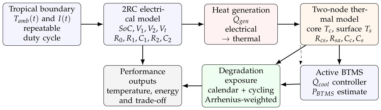
Figure 2.
Tropical heat-soak boundary condition and synthetic driving/charging duty cycle used for the three-day transient simulation. Positive current denotes discharge and negative current denotes charge.
Figure 2.
Tropical heat-soak boundary condition and synthetic driving/charging duty cycle used for the three-day transient simulation. Positive current denotes discharge and negative current denotes charge.
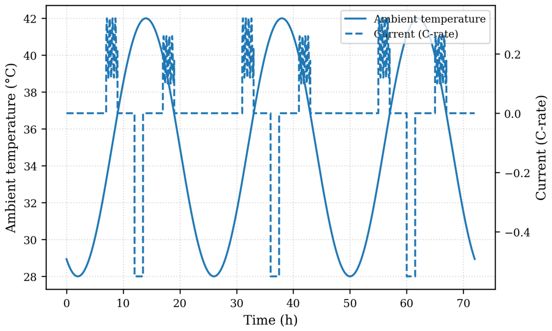
Figure 3.
Reference ohmic-resistance characteristics as functions of SoC and temperature used in the coupled 2RC-ECM.
Figure 3.
Reference ohmic-resistance characteristics as functions of SoC and temperature used in the coupled 2RC-ECM.
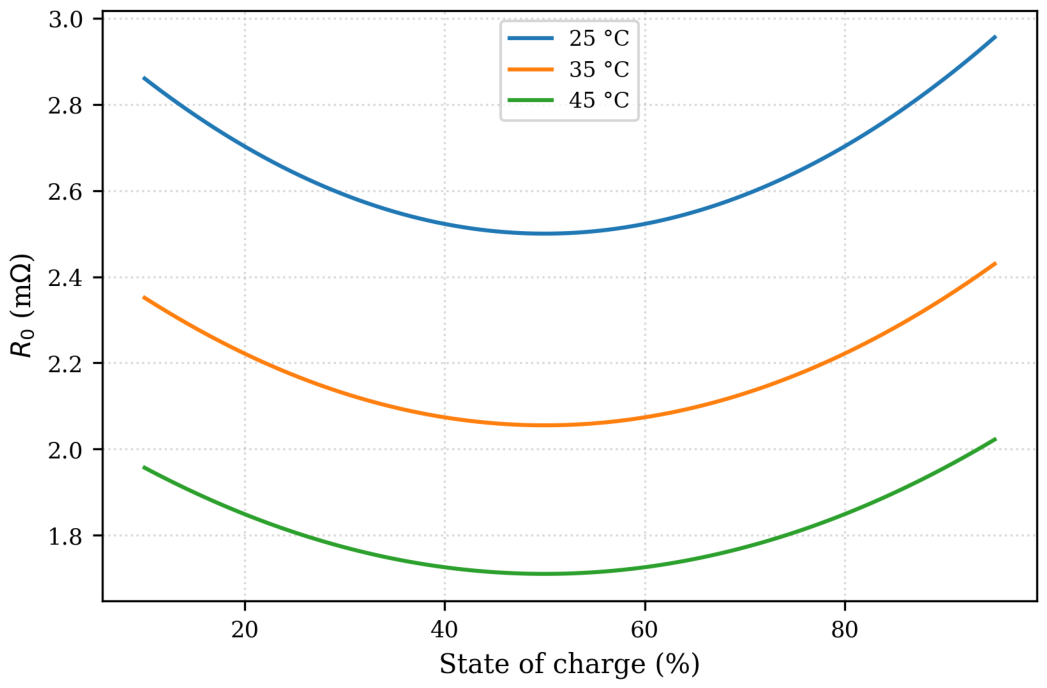
Figure 4.
Transient heat-generation components calculated from the coupled electrical model. The reversible contribution is disabled because no measured entropy-coefficient relationship is presently available.
Figure 4.
Transient heat-generation components calculated from the coupled electrical model. The reversible contribution is disabled because no measured entropy-coefficient relationship is presently available.
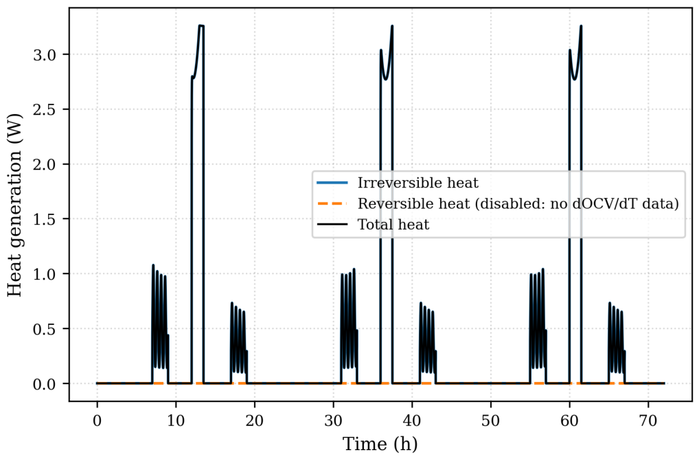
Figure 5.
Simulated core and surface temperatures under active and passive thermal management. Active cooling reduces the peak core temperature from 44.62 to 35.86 °C under the reference tropical condition.
Figure 5.
Simulated core and surface temperatures under active and passive thermal management. Active cooling reduces the peak core temperature from 44.62 to 35.86 °C under the reference tropical condition.
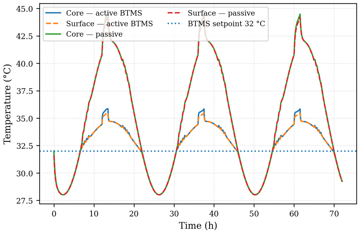
Figure 6.
Active-BTMS heat-removal rate and corresponding electrical-power demand during the three-day reference simulation.
Figure 6.
Active-BTMS heat-removal rate and corresponding electrical-power demand during the three-day reference simulation.
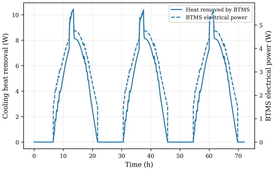
Figure 7.
Predicted core–surface temperature difference from the two-node thermal model under active and passive thermal-management conditions.
Figure 7.
Predicted core–surface temperature difference from the two-node thermal model under active and passive thermal-management conditions.
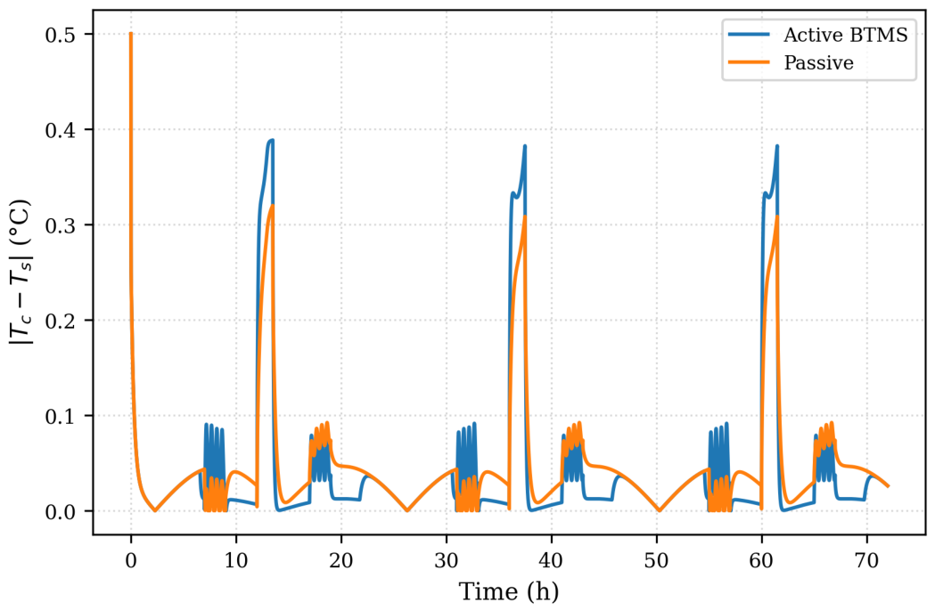
Figure 8.
Relative calendar- and cycling-degradation stress rates during the three-day tropical operating profile. The quantities represent normalized stress rates rather than percentage capacity loss.
Figure 8.
Relative calendar- and cycling-degradation stress rates during the three-day tropical operating profile. The quantities represent normalized stress rates rather than percentage capacity loss.
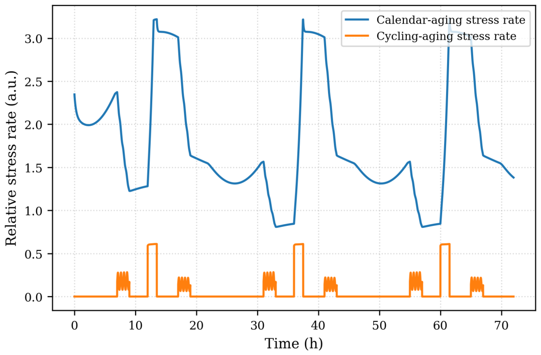
Figure 9.
Two-year equivalent cumulative degradation exposure obtained by repeating the defined three-day duty cycle under active and passive thermal-management conditions.
Figure 9.
Two-year equivalent cumulative degradation exposure obtained by repeating the defined three-day duty cycle under active and passive thermal-management conditions.
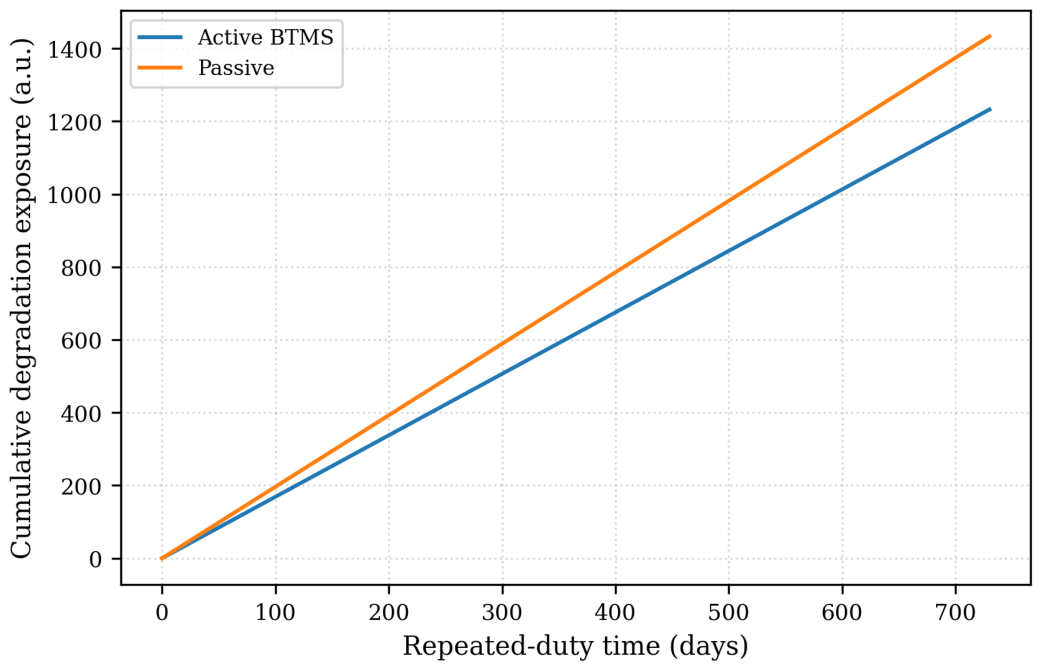
Figure 10.
Relative reduction in cumulative degradation exposure achieved by active BTMS compared with passive operation.
Figure 10.
Relative reduction in cumulative degradation exposure achieved by active BTMS compared with passive operation.
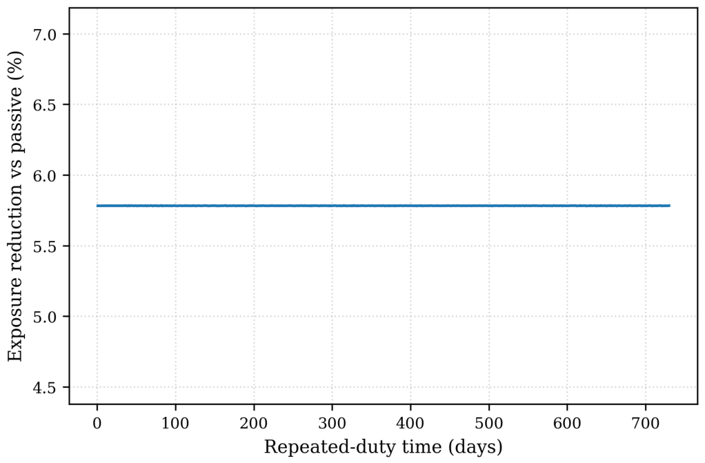
Figure 11.
Sensitivity of BTMS electrical-energy demand and maximum core temperature to changes in mean ambient temperature.
Figure 11.
Sensitivity of BTMS electrical-energy demand and maximum core temperature to changes in mean ambient temperature.
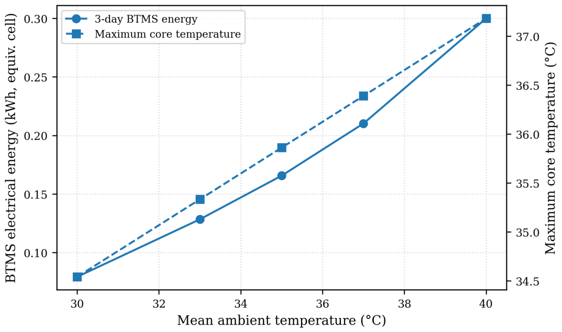
Figure 12.
Sensitivity of normalized degradation exposure and BTMS electrical-energy consumption to the selected temperature setpoint.
Figure 12.
Sensitivity of normalized degradation exposure and BTMS electrical-energy consumption to the selected temperature setpoint.
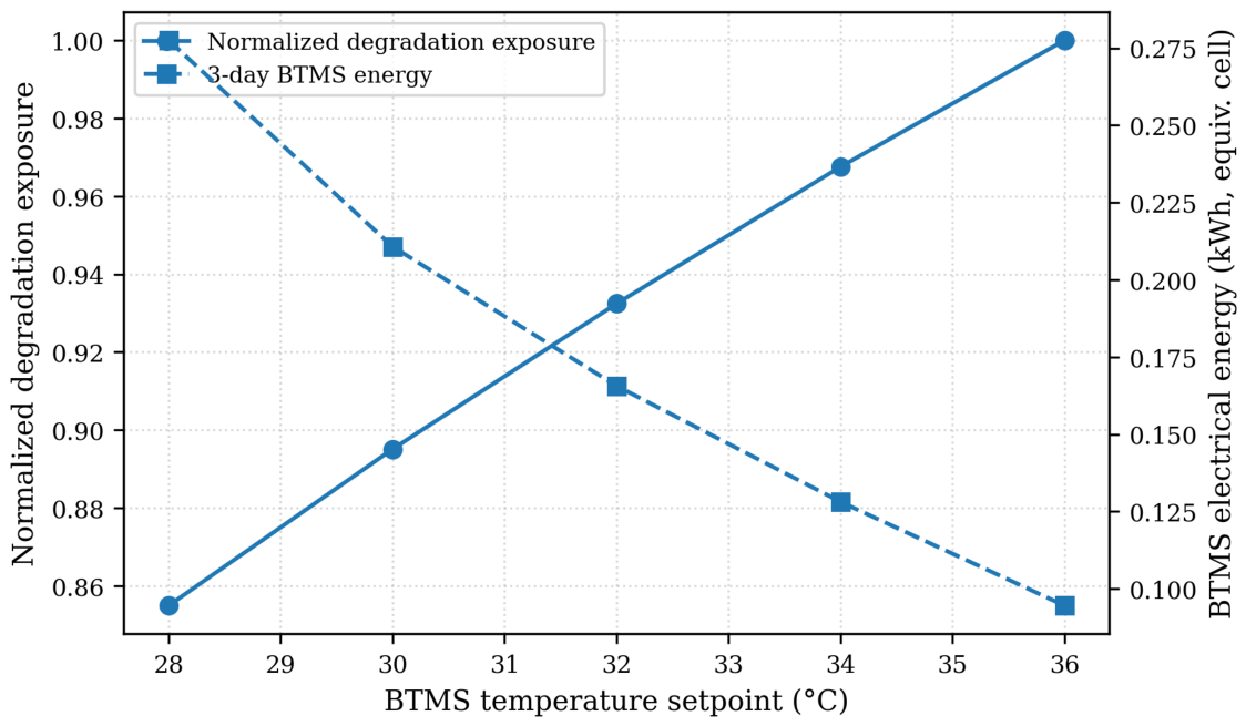
Figure 13.
Computed trade-off between BTMS electrical-energy consumption and normalized degradation exposure across the investigated temperature setpoints.
Figure 13.
Computed trade-off between BTMS electrical-energy consumption and normalized degradation exposure across the investigated temperature setpoints.
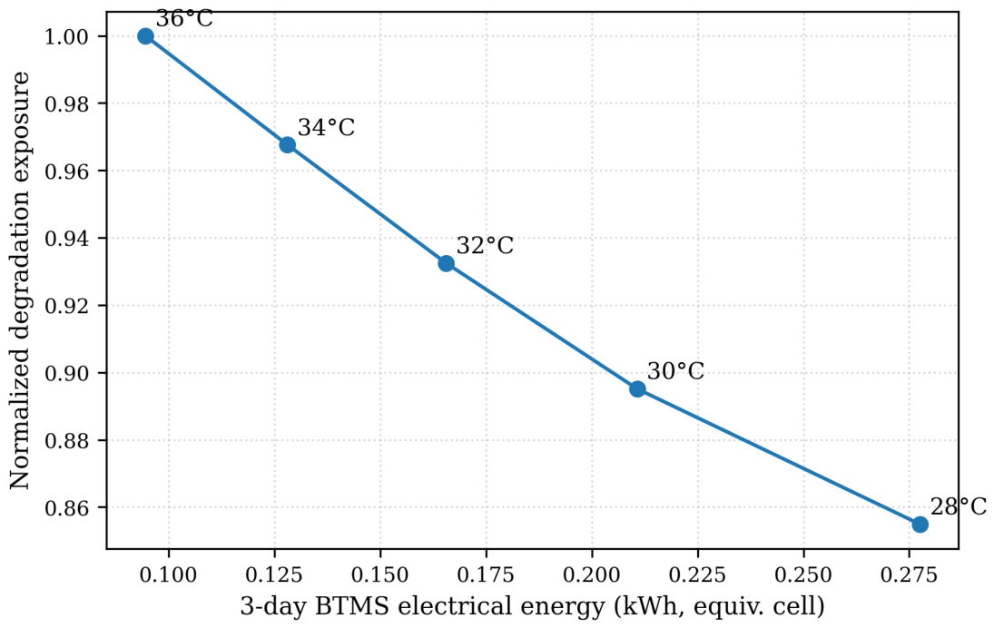

Table 1.
Reference simulation parameters. Values marked “reference” are model inputs that require cell-specific identification before quantitative experimental validation.
Table 1.
Reference simulation parameters. Values marked “reference” are model inputs that require cell-specific identification before quantitative experimental validation.
| Parameter | Symbol | Value | Role |
|---|---|---|---|
| Nominal capacity | 50 Ah | SoC integration | |
| Reference ohmic resistance | 2.5 m | ECM, reference | |
| Polarization resistance 1 | 1.2 m | ECM, reference | |
| Polarization capacitance 1 | 24,000 F | ECM, reference | |
| Polarization resistance 2 | 0.8 m | ECM, reference | |
| Polarization capacitance 2 | 90,000 F | ECM, reference | |
| Core thermal capacitance | 760 J K−1 | Thermal network, reference | |
| Surface thermal capacitance | 320 J K−1 | Thermal network, reference | |
| Core–surface resistance | 0.12 K W−1 | Thermal network, reference | |
| Surface–ambient resistance | 0.90 K W−1 | Thermal network, reference | |
| BTMS setpoint | 32 °C | Baseline control | |
| Maximum heat removal | 30 W | BTMS reference | |
| Proportional gain | 3 W K−1 | BTMS controller | |
| Reference COP | COP | 2.5 | Electrical-power estimate |
| Pump power when active | 1.5 W | Parasitic load | |
| Integration step | 10 s | Numerical integration |
Table 2.
BTMS setpoint sensitivity obtained by rerunning the complete coupled model.
| Setpoint (°C) | BTMS energy (kWh/3 d) | Maximum core T (°C) | Relative exposure |
|---|---|---|---|
| 28 | 0.277 | 33.01 | 0.855 |
| 30 | 0.211 | 34.43 | 0.895 |
| 32 | 0.166 | 35.86 | 0.932 |
| 34 | 0.128 | 37.29 | 0.968 |
| 36 | 0.095 | 38.72 | 1.000 |
Table 3.
Comparison of representative electro–thermal, aging, and BTMS studies with the present framework.
Table 3.
Comparison of representative electro–thermal, aging, and BTMS studies with the present framework.
| Study | Model / Focus | Identification / Validation | Key Relevance |
|---|---|---|---|
| Saw et al. [15] | ECM + thermal model | LFP pouch cell; experimental validation; UDDS/US06 | Electro–thermal validation under dynamic loading |
| Orcioni et al. [18] | Lumped electro–thermal model | Parameter extraction; climatic-chamber validation | Reduced-order cell/pack simulation |
| Schmalstieg et al. [5] | Calendar + cycling aging | Accelerated aging tests; temperature and SoC effects | Calibrated lifetime prediction |
| Naguib et al. [9] | 2RC electro–thermal model | HPPC identification; multi-temperature dynamic validation | SoC/temperature-dependent 2RC modeling |
| Shi et al. [11] | Layered electro–thermal ECM | Internal-temperature estimation | Core/internal temperature representation |
| Present study | 2RC + thermal + BTMS + aging exposure | Tropical heat-soak and setpoint sensitivity; numerical study | Thermal–energy–degradation trade-off |
Disclaimer/Publisher’s Note: The statements, opinions and data contained in all publications are solely those of the individual author(s) and contributor(s) and not of MDPI and/or the editor(s). MDPI and/or the editor(s) disclaim responsibility for any injury to people or property resulting from any ideas, methods, instructions or products referred to in the content. |
© 2026 by the authors. Licensee MDPI, Basel, Switzerland. This article is an open access article distributed under the terms and conditions of the Creative Commons Attribution (CC BY) license (http://creativecommons.org/licenses/by/4.0/).
Copyright: This open access article is published under a Creative Commons CC BY 4.0 license, which permit the free download, distribution, and reuse, provided that the author and preprint are cited in any reuse.