

Submitted:
24 September 2026
Posted:
28 September 2026
You are already at the latest version
Abstract
Purpose: To classify optical filters with different filtering levels according to their algorithmic complexity and to evaluate their effects on visual acuity (VA). The Block Decomposition Method (BDM) was applied to classify optical filters based on their estimated algorithmic complexity. Methods: VA was measured in all participants. Optical filters were analyzed using conventional statistical methods together with the BDM to characterize their algorithmic complexity. Results: Selective absorption filters exhibited a progressive reduction in transmittance within the blue spectral region (380–500 nm), accompanied by a shift of the cutoff wavelength toward longer wavelengths and a reduction in effective bandwidth, while maintaining relatively stable overall visible transmittance. Shannon entropy analysis revealed a progressive increase in statistical diversity as filter treatment time increased. In contrast, the algorithmic complexity estimated using the BDM exhibited a non-linear behavior, reaching its highest values in filters treated for 1 and 2 minutes. VA analysis performed on 235 eyes showed that the algorithmic complexity of visual responses depended on the visual function evaluated. Resolution acuity exhibited a decreasing trend in the estimated algorithmic complexity of its computational representation, whereas alignment acuity showed an overall increase across filter conditions. Detection acuity displayed non-linear changes, while recognition acuity included the highest individual nBDM value among the visual functions evaluated. Conclusions: Algorithmic complexity provides a complementary approach to conventional statistical methods for the analysis of ophthalmic filters and visual responses. The results indicate that statistical diversity and estimated algorithmic complexity characterize distinct and complementary properties of the computational representations analyzed. Selective absorption filters were associated with changes in the computational organization of the transmittance spectra and with differences in the computational representations of visual responses. BDM provided information about algorithmic organization that was complementary to conventional descriptive statistics and Shannon entropy, supporting its potential use as an additional computational tool for the characterization of photoselective filters and their relationship with visual performance.
Keywords:
algorithmic complexity
; Block Decomposition Method
; BDM
; selective absorption filters
; photoselective filters
; UV–Vis spectrophotometry
; visual acuity
; Shannon entropy
; human vision
Introduction
Absorption filters are widely used for spectral band selection within the visible region. Their primary function is to selectively absorb specific portions of the visible spectrum.
Increasing spectral absorption reduces the absolute amount of light reaching the retinal photoreceptors, thereby decreasing contrast sensitivity (CS) and VA. (Guirao Piñera, 1999) The minimum visible stimulus is determined not only by its angular size but also by the surface luminance of the test stimulus, the amount of luminous energy absorbed by the photoreceptors, and the observer’s visual sensitivity. VA increases approximately with the logarithm of illumination intensity (Martín Herranz & Vecilla Antolínez, 2011) and decreases with the square root of contrast (Rubin & Legge, 1989). Likewise, visual performance improves as the surface luminance of the optotype increases. (Mico, 2011)
Previous studies have shown that VA is slightly lower under blue illumination, whereas visual acuity measured under red and green illumination is comparable to that obtained under white light. (Capilla et al., 1993)
Attenuation or removal of specific portions of the visible spectrum directly modifies chromatic variables, thereby affecting both the intensity and chromaticity of the transmitted spectrum.
The hue of a visual stimulus can be defined by three independent variables corresponding to the luminous energy of three spectral lights (Mico, 2011; Montés-Micó, 2011). Consequently, variations in the intensity of different wavelengths produce changes in color perception. (Bonnin Arias et al., 2015)
These considerations highlight the importance of comparing different optical filters, since differences in manufacturing technologies may result in significant variations in the optical and visual variables evaluated. Spectral filtering is therefore expected to produce perceptual changes.
The present study aimed to determine the relationship between the absorption spectra of optical filters and VA. In addition, optical filters with different filtering levels were classified according to their algorithmic complexity by applying the BDM.
Methods
Study Design and Sampling
This was a prospective, descriptive, quasi-experimental, correlational study with a cross-sectional, non-probability sampling design. Non-probability sampling was used for both filter selection and participant recruitment. Quota sampling was used to select the optical filters, whereas convenience or purposive sampling was used to recruit the test participants. The inclusion criterion for the optical filters was a minimum mean absorption of 20% over the 380–500 nm spectral range. For the purposes of the spectral analysis, absorption was operationally estimated from transmittance as . This operational definition does not separately account for reflectance losses. Participant inclusion criteria were a corrected refractive status, absence of oculomotor disorders, age between 18 and 35 years, absence of diseases affecting VA, CD, CS, or stereoscopic visual acuity (SVA), and provision of informed consent. The exclusion criteria for optical filters were ophthalmic lenses incorporating photochromic treatments or having dioptric power. Participant exclusion criteria were ocular pathology affecting VA; abnormalities in color discrimination (CD); reduced CS at high, intermediate, or low spatial frequencies; binocular vision abnormalities; or SVA worse than 200 arcsec.
The elimination criteria were optical filters whose mean transmittance values differed by less than 5% from those of another filter, and participants who did not complete the full test battery.
Algorithmic Information Theory (AIT)
AIT provides a formal framework for studying the information content of finite objects based on the length of the shortest computational description capable of generating them. Unlike classical statistical measures, which describe the distribution of symbols or values, AIT focuses on the existence of generative mechanisms that can account for the observed structure through programs of minimum length.
Within this framework, the Kolmogorov complexity of an object is defined as the length of the shortest program that, when executed on a universal Turing machine, produces that object and halts. Because this quantity is uncomputable in the general case, computable estimators of algorithmic complexity are used in experimental applications.
One of the most widely used methods is the BDM, developed by Zenil and colleagues. BDM approximates algorithmic complexity by combining local estimates obtained using the Coding Theorem Method (CTM) with a logarithmic penalty associated with the repetition of blocks.
It is important to distinguish between statistical entropy, algorithmic randomness, computational structure, and algorithmic complexity, as these represent different properties of the same object. High entropy indicates statistical diversity, whereas high algorithmic complexity reflects low compressibility of the representation being analyzed. These properties are not equivalent and may evolve independently. (Chaitin, 1969; Kolmogorov, 1968; Solomonoff, 1964)
Fundamental Concepts
Algorithmic Complexity (): Also known as Kolmogorov complexity, it is defined as the length of the shortest computer program () that, when executed on a universal Turing machine (), generates a specific string () and halts. If a string cannot be described by a program shorter than the string itself, it is considered algorithmically random. A critical aspect is that is uncomputable because of the halting problem; therefore, approximations are used in practice.
Because is not computable for an arbitrary object, approximations are used in experimental applications. In this study, BDM is used, combining local estimates obtained through CTM with a logarithmic penalty associated with the repetition of blocks.
Algorithmic Probability (): This is a measure that estimates the probability that a random program will produce a specific string when executed. Unlike classical probability, it replaces the random generation of outcomes with the random generation of programs. The CTM establishes a direct connection between this probability and algorithmic complexity: strings with higher algorithmic probability are those with lower algorithmic complexity.
Origin and Motivation
Key contributors: The foundations of this theory were established by scientists such as Solomonoff, Kolmogorov, Chaitin, and Levin.
Scientific motivation: The theory emerged from the human drive to explain observed phenomena and to understand that apparent chaos may often arise from underlying causes or order. From the perspective of AIT, an important task is to determine whether an observed pattern can be explained by simple generative mechanisms, predominantly random processes, or a combination of both. This distinction makes it possible to differentiate statistical diversity from the underlying computational structure.
Limitations of previous metrics: Although tools such as Shannon entropy are widely used, they have limitations; for example, entropy depends on choices regarding the granularity of the representation and detects statistical regularities rather than algorithmic ones. (Shannon, 1948; Zenil, Badillo, et al., 2018) AIT emerged as a framework for determining whether a phenomenon is intrinsically random or possesses a more concise description.
Shannon entropy characterizes the statistical diversity of a distribution of values, whereas BDM approximates the algorithmic complexity of the complete representation of an object. Therefore, the two measures describe complementary properties and do not necessarily exhibit a monotonic relationship.
What Is It Used for?
Assessing algorithmic randomness: AIT provides a framework that goes beyond statistical entropy and traditional compression algorithms for evaluating the information content of an object.
Revealing hidden patterns: It can identify cases in which objects that appear statistically random may nevertheless possess a well-defined algorithmic structure, as illustrated by sequences such as the Thue–Morse sequence.
Analysis of complex systems: Through methods such as BDM, the algorithmic complexity of large systems can be estimated by decomposing them into smaller components. This approach can be applied to objects ranging from binary sequences to graph adjacency matrices. (Zenil, Badillo, et al., 2018; Zenil et al., 2015)
Investigation of generative mechanisms: AIT provides tools for exploring the possible generative mechanisms underlying observed systems, thereby contributing to a deeper understanding of complex phenomena in natural and technological systems.
In summary, AIT provides a framework for characterizing the algorithmic complexity underlying apparently simple, structured, or random phenomena.
BDM is calculated by decomposing a large object, such as a binary string, matrix, or graph, into smaller and more manageable blocks and estimating its overall complexity from the algorithmic complexity and multiplicity of its constituent blocks.
General Formula
For a sequence s, the BDM value is calculated using the following sum:
(Zenil, Badillo, et al., 2018)
where:
: the i-th subsequence or block obtained after partitioning the original object.
: the multiplicity of the corresponding subsequence; that is, the number of times that specific block occurs within the complete object.
: the approximate algorithmic complexity value assigned to each block, previously estimated using the CTM with Turing machines consisting of states and symbols.
: the logarithm of the block multiplicity, usually with for binary objects, which accounts for repeated occurrences of the same pattern. (Delahaye & Zenil, 2011)
Steps for Calculation
In practice, the BDM procedure involves the following general steps:
Object partitioning: The system, such as a string or matrix, is divided into smaller blocks of a predefined size.
Selection of the partitioning strategy: The resulting BDM estimate may vary depending on how the blocks and remaining elements are handled:
Ignore-remainders partitioning: Incomplete blocks or remaining elements that do not fill the specified block size are discarded.
Overlapping partitioning: A sliding window with overlap is used to generate successive blocks, allowing neighboring regions of the object to be included in the decomposition.
Recursive partitioning: The object is recursively decomposed to reduce the number of incomplete blocks while retaining blocks of the largest possible size.
CTM value lookup: Algorithmic complexity estimates for the resulting blocks are obtained from precomputed CTM values, such as those available through the OACC calculator or implemented in the PyBDM library.
Aggregation of values: The CTM value of each unique block is combined with the logarithm of its multiplicity, and these contributions are summed to obtain the BDM estimate.
Application to Multidimensional Objects
For graphs represented by adjacency matrices or for two-dimensional arrays, BDM can be extended by partitioning the object into smaller submatrices and applying the corresponding CTM-based complexity estimates to the resulting two-dimensional blocks.
In summary, BDM combines local CTM-based estimates of algorithmic complexity with a logarithmic term accounting for block multiplicity. Thus, repeated patterns contribute differently from unique or algorithmically complex blocks, allowing BDM to characterize aspects of the computational organization of an object that are not captured solely by conventional statistical measures such as Shannon entropy.
Operational Definitions
Computational representation of the spectrum. In this study, each transmittance spectrum is represented as an ordered sequence of transmittance values associated with their corresponding wavelengths. For BDM analysis, this sequence is normalized, discretized, and treated as a finite computational object that can be analyzed using tools from AIT.
Structure. In the context of the present study, the term structure refers to the computational organization of the discretized representation of the transmittance spectrum; that is, the sequential arrangement of the symbols obtained after the discretization process. This definition does not refer to the physical, chemical, or microscopic structure of the filter material, but exclusively to the representation used to estimate its algorithmic complexity.
Estimated algorithmic complexity. In this study, algorithmic complexity refers to the approximation obtained using BDM, which estimates Kolmogorov complexity from local decompositions based on CTM. Consequently, the reported values represent computable estimates of algorithmic complexity rather than exact Kolmogorov complexity, which is uncomputable in the general case.
Algorithmic randomness. In the present study, algorithmic randomness is understood as the extent to which a computational representation cannot be described by a program significantly shorter than the representation itself. This concept differs from statistical randomness as quantified by Shannon entropy, since the two characterize distinct properties of the same representation.
The definitions above establish the operational meaning of the main concepts used in this study and delimit the scope of their interpretation. Consequently, subsequent references to complexity, structure, or randomness should always be understood within the context of the computational representation of the analyzed spectra and not as intrinsic physical properties of the filter materials.
Rationale for the Use of BDM in the Analysis of Transmittance Spectra
Transmittance spectra obtained by UV–Vis spectrophotometry are signals ordered as a function of wavelength. Although these spectra are traditionally analyzed using statistical parameters such as mean transmittance, standard deviation, or Shannon entropy, these metrics primarily describe the distribution of values rather than the organization of the signal across the spectral domain.
In this study, each transmittance spectrum is considered a finite computational object. The spectral signal was represented as a discrete sequence of transmittance values ordered by wavelength, thereby enabling the application of tools from AIT.
Under this representation, BDM provides a computable approximation of the algorithmic complexity of the spectrum by decomposing the sequence into blocks, estimating the local complexity of each block using CTM, and accounting for the repetition of patterns within the representation. Consequently, BDM evaluates the algorithmic compressibility of the spectral organization rather than solely the statistical diversity of its values.
This characteristic makes BDM complementary to Shannon entropy. Two spectra may exhibit similar transmittance distributions and, consequently, comparable entropy values, while differing in algorithmic complexity if the sequential organization of their values is consistent with different generative mechanisms. Therefore, the combined use of both metrics provides a more comprehensive characterization of the computational organization of the transmittance spectra of the photoselective filters analyzed. (Crutchfield & Young, 1991; Zenil et al., 2020)
Shannon Entropy
Question: How statistically diverse or uncertain are the values?
Example:
Spectrum A Low entropy.
Spectrum B High entropy.
However, Shannon entropy does not necessarily reveal whether the observed sequence follows an underlying algorithmic rule.
Standard Deviation
Question: How much do the data values vary around their mean?
Standard deviation quantifies the dispersion of the values but does not characterize their sequential organization.
It does not distinguish: from
Fast Fourier Transform (FFT)
Question: What frequency components are present in the signal?
The FFT is effective for detecting periodic components but does not directly characterize:
- Symmetries
- Complex repetitions
- Hierarchical structures
(Cooley & Tukey, 1965; Shannon, 1948; Zenil, Hernández-Orozco, et al., 2018)
Block Decomposition Method (BDM)
Question: How complex is the algorithmic description of this spectrum?
Examples:
Spectrum 1 Very low algorithmic complexity.
Spectrum 2 High entropy and low BDM complexity because the representation contains a simple repetitive pattern .
Spectrum 3 High BDM complexity; no simple generative rule is apparent in the representation.
Statistical Analysis
General Descriptive Statistics of Transmittance. The descriptive parameters of the transmittance spectra were calculated over the 380–780 nm wavelength range for the optical filters included in the study.

Table 1.
Descriptive Statistics of Transmittance (%) According to Filter Treatment Time.
| Statistical Parameter | ||||
|---|---|---|---|---|
| Filter treatment time (immersion pigmentation) |
30 s | 1 min | 2 min | 3 min |
| Mean | 73 | 72 | 66 | 66 |
| Median | 79 | 79 | 77 | 81 |
| Mode | 81 | 78 | 80 | 83 |
| Standard Deviation | 18 | 22 | 25 | 30 |
| Variance | 306 | 500 | 633 | 887 |
| Minimum | 34 | 26 | 12 | 7 |
| Maximum | 99 | 98 | 98 | 98 |
| Range | 65 | 72 | 86 | 91 |
| Coefficient of Variation (CV) | 20% | 24% | 31% | 38% |
Interpretation and Observations of the Analysis
Central Tendency (Mean and Median): Filters and showed the highest mean transmittance values (>71%), indicating greater overall light transmission across the measured spectral range. In contrast, and were the most restrictive filters, with mean transmittance values of approximately 66%.
Stability and Dispersion: Filter exhibited the lowest variability across the evaluated spectral range, with the smallest standard deviation (18) and coefficient of variation (CV = 20%). In contrast, exhibited the greatest variability (CV = 38%) and the widest range (91), reaching a maximum transmittance of 98% while decreasing to a minimum of 7%.
Mode Analysis: The most frequently occurring transmittance values (modes) were concentrated in the upper portion of the transmittance scale for all filters (≥78%). This pattern is consistent with the high-transmittance plateaus observed in selective optical filters beyond their main absorption region.
Normality Tests
Table 2.
Normality tests for the transmittance distributions of the four optical filters.
| Kolmogorov–Smirnov | Shapiro–Wilk | |||
| Filter | D | p-value | W | p-value |
| 0.2359 | 6.90 × 10⁻¹⁰² | 0.8424 | 2.83 × 10⁻⁴¹ | |
| 0.2682 | 4.49 × 10⁻¹³² | 0.8097 | 3.89 × 10⁻⁴⁴ | |
| 0.2823 | 1.54 × 10⁻¹⁴⁶ | 0.7997 | 6.24 × 10⁻⁴⁵ | |
| 0.3020 | 4.20 × 10⁻¹⁶⁸ | 0.7598 | 8.37 × 10⁻⁴⁸ | |
Kolmogorov–Smirnov Test
: The distribution is normal. : The distribution is not normal.
All p-values were <0.001. Therefore, the null hypothesis of normality () was rejected for all four filters.
Shapiro–Wilk Test
All p-values were <0.001, indicating significant departures from normality. Therefore, the null hypothesis of normality () was rejected for all four filters.
Because both tests indicated significant departures from normality, non-parametric statistical methods were used for subsequent comparisons. However, because spectral transmittance values are ordered by wavelength, adjacent observations may exhibit spectral dependence. Therefore, the inferential results should be interpreted within the context of paired spectral measurements rather than as independent observations.
Friedman Test
The hypotheses were defined as follows:
:There are no differences among the filters.
:At least one filter differs from the others.
The Friedman test yielded:
,
Therefore, was rejected, indicating statistically significant differences among the filters.
Pairwise Wilcoxon Signed-Rank Tests
All six possible pairwise comparisons were performed. A Bonferroni correction was applied to account for multiple comparisons.
Table 3.
Pairwise Comparisons of Spectral Transmittance Among Filters Using the Wilcoxon Signed-Rank Test with Bonferroni Correction. Note. The Bonferroni-adjusted significance threshold was p < 0.00833 (α = 0.05/6). All pairwise comparisons remained statistically significant after correction.
Table 3.
Pairwise Comparisons of Spectral Transmittance Among Filters Using the Wilcoxon Signed-Rank Test with Bonferroni Correction. Note. The Bonferroni-adjusted significance threshold was p < 0.00833 (α = 0.05/6). All pairwise comparisons remained statistically significant after correction.
| Comparison | W | p-value |
| vs | 803773.5 | 2.54 × 10⁻¹⁸ |
| vs | 73258.0 | 9.70 × 10⁻²⁸³ |
| vs | 637760.0 | 1.64 × 10⁻³⁷ |
| vs | 105870.0 | 7.90 × 10⁻²⁶⁰ |
| vs | 378572.0 | 9.09 × 10⁻¹⁰⁷ |
| vs | 883423.0 | 7.81 × 10⁻⁶ |
All pairwise comparisons remained statistically significant after Bonferroni correction, indicating significant differences between each pair of filters.
Spearman Rank Correlations
Spearman’s rank correlation coefficients were calculated to assess the monotonic relationships among the spectral transmittance profiles of the four filters.
Table 4.
Spearman Rank Correlation Matrix for the Spectral Transmittance Profiles of the Four Filters.
Table 4.
Spearman Rank Correlation Matrix for the Spectral Transmittance Profiles of the Four Filters.
| 1.000 | 0.873 | 0.964 | 0.950 | |
| 0.873 | 1.000 | 0.903 | 0.901 | |
| 0.964 | 0.903 | 1.000 | 0.971 | |
| 0.950 | 0.901 | 0.971 | 1.000 |
All correlations were positive and very strong, with Spearman’s ρ ranging from 0.873 to 0.971. The strongest relationship was observed between F3 and F4 (ρ = 0.971), whereas the lowest, although still very strong, was observed between F1 and F2 (ρ = 0.873).
Summary of Statistical Results
The statistical results indicate that the four filters exhibited significantly different spectral transmittance profiles while maintaining very strong positive monotonic relationships across the analyzed wavelengths.
Table 5.
Summary of Statistical Analyses of the Spectral Transmittance Profiles.
| Test | Result | Conclusion |
| Kolmogorov–Smirnov | p < 0.001 for all filters | Non-normal distributions |
| Shapiro–Wilk | p < 0.001 for all filters | Non-normal distributions |
| Friedman | χ2 = 1614.043; p < 0.001 | Significant differences among filters |
| Wilcoxon signed-rank tests with Bonferroni correction | All pairwise comparisons significant | All filters differed significantly from one another |
| Spearman | ρ = 0.873–0.971 | Very strong positive correlations |
Instrumental Analysis Results
Spectral Characteristics of the Selective Absorption Filters
Figure 1.
Transmittance Spectra of the Selective Absorption Filters over the 380–780 nm Wavelength Range.
Figure 1.
Transmittance Spectra of the Selective Absorption Filters over the 380–780 nm Wavelength Range.
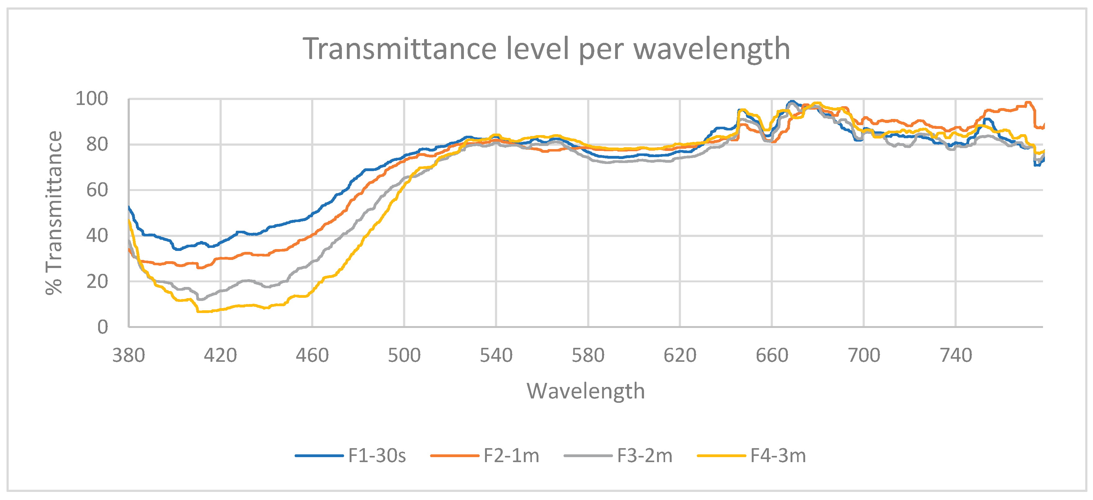
Table 6.
Summary of Spectral Transmittance and Absorption Parameters of the Selective Absorption Filters. Note. Transmittance was measured using UV–Vis spectrophotometry. Mean absorption over the 380–500 nm range was operationally estimated as \( A(\%) = 100 - T(\%)\) ; reflectance losses were not separately accounted for.
Table 6.
Summary of Spectral Transmittance and Absorption Parameters of the Selective Absorption Filters. Note. Transmittance was measured using UV–Vis spectrophotometry. Mean absorption over the 380–500 nm range was operationally estimated as \( A(\%) = 100 - T(\%)\) ; reflectance losses were not separately accounted for.
| Parameter | ||||
|---|---|---|---|---|
| Mean visible transmittance (%) | 72.93 | 71.74 | 65.58 | 65.76 |
| Mean transmittance, 380–500 nm (%) | 48.63 | 39.80 | 28.97 | 21.21 |
| Mean transmittance, 500–780 nm (%) | 82.66 | 84.56 | 80.25 | 83.60 |
| Mean absorption, 380–500 nm (%) | 51.37 | 60.20 | 71.03 | 78.79 |
| 50% transmittance wavelength, (nm) | 381.17 | 472.54 | 482.37 | 491.57 |
| Effective bandwidth (nm) | 399.77 | 308.38 | 297.74 | 288.94 |
Mean Visible Transmittance (380–780 nm)
Although filters – progressively attenuated a larger portion of the blue spectral region, overall visible transmittance decreased relatively modestly. Mean visible transmittance decreased from 72.93% for to 65.76% for , corresponding to a difference of 7.17 percentage points.
This indicates that the filters progressively attenuated the blue spectral region while maintaining relatively high overall visible transmittance.
From a clinical perspective, this behavior may be relevant because it reduces the transmission of short-wavelength radiation while preserving a substantial proportion of overall visible light.
Mean Transmittance over 380–500 nm
A pronounced progressive reduction in mean transmittance was observed over the 380–500 nm spectral range. Mean transmittance decreased from 48.63% for to 21.21% for .
Thus, transmitted approximately 44% of the amount transmitted by within this spectral range:
This finding confirms that the main differences among the filters were concentrated in the blue–violet region of the spectrum.
Mean Transmittance over 500–780 nm
The four filters exhibited similar mean transmittance values over the 500–780 nm spectral range, ranging from 80.25% to 84.56%. The maximum difference among the filters was therefore 4.31 percentage points.
This indicates that the major differences among the filters occurred primarily at shorter wavelengths, whereas transmittance across the green-to-red region remained comparatively similar.
Cutoff Wavelength (λ50)
The value progressively shifted toward longer wavelengths, increasing from 381.17 nm for to 491.57 nm for . This indicates that progressively longer wavelengths were required for the filters to reach 50% transmittance.
The overall shift between and was: 491.57−381.17=110.40 nm representing a substantial shift toward longer wavelengths within the blue–cyan spectral region.
Effective Bandwidth
A progressive reduction in effective bandwidth was observed as treatment time increased. Effective bandwidth decreased from 399.77 nm for to 288.94 nm for , corresponding to a reduction of:
Thus, exhibited an effective bandwidth approximately 28% narrower than that of , consistent with an increase in spectral selectivity.
Application of BDM to Optical Filters
Within the computational representation adopted in this study, BDM can be used to characterize several properties of the transmittance spectra:
Algorithmic complexity: How complex is the computational representation of the spectrum?
Computational organization: To what extent does the discretized spectral representation contain identifiable algorithmic regularities?
Algorithmic randomness: To what extent does the spectral representation lack a substantially shorter algorithmic description?
Changes associated with filter treatment: Does the computational organization of the transmittance spectrum change as a function of filter treatment?
Filter Classification
For example, optical filters may include neutral-density filters, selective filters, notch filters, and multilayer filters. Many of these filters may exhibit similar mean transmittance values. However, even when filters have comparable mean transmittance, differences in the computational organization of their spectral representations may be revealed using measures of algorithmic complexity. (Zenil, Badillo, et al., 2018; Zenil et al., 2020)
In this context, BDM is proposed as a method for the classification of optical filters.
Computational Processing of the Spectra
The transmittance spectra obtained by UV–Vis spectrophotometry were represented as discrete sequences of transmittance values ordered by wavelength, thereby constituting finite computational objects suitable for BDM analysis. Computational processing was performed using Python.
Data Discretization for BDM Calculation
Prior to estimating algorithmic complexity using BDM, the continuous data were subjected to normalization and discretization.
First, each variable was normalized using a min–max transformation to scale all values to the interval [0,1]:
where:
is the original value, and and are the minimum and maximum values of each variable, respectively.
The normalized values were subsequently discretized using a binary alphabet (NSYMBOLS = 2). This configuration was selected because it is fully supported by the CTM tables implemented in PyBDM and avoids the coverage limitations observed with larger alphabets.
Algorithmic complexity of the spectra was estimated using the BDM implementation available in the PyBDM Python library. Both absolute BDM complexity (BDM) and normalized BDM complexity (nBDM) were calculated.
For binary discretization, the normalized interval [0,1] was divided into two regions:
Normalized interval Assigned symbol
| 0 | |
| 1 |
Symbol assignment was performed using the numpy.digitize() function, generating a binary integer sequence that was subsequently used as input to the BDM algorithm.
Python Implementation
In Python, the procedure was implemented as follows:
NSYMBOLS = 2
bins = np.linspace(0,1,NSYMBOLS+1)
y = np.digitize(x_norm,bins)-1
y[y==NSYMBOLS]=NSYMBOLS-1
The resulting discretization produces a sequence such as:
| Normalized values | Discretized sequence |
| 0.12, 0.36, 0.48, 0.55, 0.71, 0.92 | 0, 0, 0, 1, 1, 1 |
This discrete representation constitutes the input required by PyBDM to estimate algorithmic complexity by decomposing the sequence into blocks and comparing these blocks with precomputed CTM values.
Why Were Only Two Symbols Used?
The choice of NSYMBOLS = 2 was based on both methodological and computational considerations:
- It ensures compatibility with the CTM tables available in PyBDM.
- It avoids warnings related to patterns not represented in the CTM database, which were observed when using alphabets of four or more symbols.
- It provides a consistent and reproducible procedure for estimating algorithmic complexity.
- It reduces excessive fragmentation of the data when the number of observations is limited.
Consequently, binary discretization provided a standardized representation of the overall organization of the signals while ensuring compatibility and computational stability in the BDM analysis.
Methodological Sensitivity Analysis
The estimates obtained using BDM depend on the computational representation of the object being analyzed and on several methodological parameters, including the alphabet size used for discretization (NSYMBOLS), the partitioning strategy, and the CTM tables used to approximate algorithmic complexity. In the present study, NSYMBOLS = 2 was selected because this configuration is fully supported by the CTM tables implemented in PyBDM, thereby avoiding the coverage issues observed with larger alphabets and facilitating reproducibility of the calculations.
Although a systematic sensitivity analysis across different discretization configurations or partitioning strategies was not performed, the conclusions of the present study should be interpreted within the methodological framework described herein. Accordingly, future studies should evaluate the stability of BDM estimates under variations in these parameters to determine the robustness of the results and the extent to which they depend on the selected computational representation.
It should also be noted that the estimates obtained using BDM constitute computable approximations of algorithmic complexity and do not represent exact Kolmogorov complexity, which is uncomputable in the general case.
The one-dimensional analysis () was applied directly to the spectral sequence.
The two-dimensional analysis () was performed on a matrix representation derived from the spectral sequence.
To facilitate comparison among computational objects, normalized BDM values (nBDM) were also calculated.
For the two-dimensional analysis (), each spectral sequence was reshaped into a 37 × 56 matrix (2072 samples), thereby preserving the total number of observations. This representation enabled application of the two-dimensional BDM algorithm to a matrix structure derived from the original spectral sequence.
Reshaping the spectral sequence into a 37 × 56 matrix was based on a strictly computational criterion. This configuration allowed all 2072 experimental observations to be represented without removing data or introducing artificial values through padding, thereby preserving the complete set of measurements acquired during spectrophotometric analysis. The matrix representation did not alter the original transmittance values; rather, it constituted a reorganization of the same dataset required for application of the two-dimensional BDM algorithm.
It should be emphasized that the resulting matrix does not represent the physical spatial organization of the optical filter. Instead, it constitutes solely a computational representation of the transmittance spectrum used to estimate algorithmic complexity through BDM. Consequently, conclusions derived from the two-dimensional analysis should be interpreted within the context of this computational representation and not as intrinsic geometric, spatial, or structural properties of the material being analyzed.
Although alternative matrix arrangements preserving the same number of observations could be used for two-dimensional analysis, a systematic assessment of the sensitivity of BDM to different matrix configurations was beyond the scope of the present study and represents a direction for future research.
In addition to absolute BDM values, the corresponding normalized values (nBDM) were calculated to provide a relative measure of algorithmic complexity.
The analysis was performed using PyBDM version 0.1.0 (2019-09-22), developed by Szymon Talaga, Kostas Tsampourakis, and Paweł Weroński.
As a reference statistical measure, Shannon entropy was calculated from the discretized sequences using a base-2 logarithm. This metric was used to compare the statistical diversity of the spectra with their algorithmic complexity as estimated by BDM.
All computational processing was implemented in Python using the PyBDM library and executed in a Google Colaboratory environment.
Table 7.
Computational Environment and Software Versions Used in the Analysis.
| Software / Metric | Version / Configuration |
| Python | 3.12.13 |
| PyBDM | 0.1.0 |
| NumPy | 2.0.2 |
| pandas | 2.2.2 |
| SciPy | 1.16.3 |
| Shannon entropy | Base 2 |
Methodological Limitations of the BDM Implementation
The BDM implementation used in this study corresponds to the PyBDM library, which provides a computable approximation of algorithmic complexity by combining the CTM with block decomposition of the object. Consequently, the resulting values represent estimates of algorithmic complexity rather than exact Kolmogorov complexity, which is uncomputable in the general case.
Furthermore, the accuracy of these estimates depends on the computational representation of the object being analyzed and on the parameters used during processing, including data discretization, alphabet size, partitioning strategy, and the coverage of the CTM tables available in PyBDM. Therefore, the resulting values should be interpreted within the methodological framework described in this study and not as absolute quantities independent of the representation used.
It should also be noted that the CTM tables implemented in PyBDM are precomputed for specific symbol configurations and block sizes. This imposes practical constraints on the discretization procedure and may limit the evaluation of representations using larger alphabets or alternative configurations without requiring additional approximations.
Finally, BDM is an estimator of algorithmic complexity and not a method for directly inferring causal relationships. Consequently, differences observed among computational representations should be interpreted as evidence consistent with generative mechanisms of different algorithmic complexity, without directly attributing them to underlying physical or causal mechanisms.
Uncertainty of the Estimates
nBDM values obtained in this study are point estimates derived from the computational representation employed. Confidence intervals or uncertainty estimates based on resampling procedures, such as bootstrapping, were not calculated. Consequently, small differences between nBDM values should be interpreted with caution and considered within the exploratory context of the present study.
Comparison of BDM and Shannon Entropy
Table 8.
Comparison of BDM-Based Algorithmic Complexity and Shannon Entropy Across Selective Absorption Filters.
Table 8.
Comparison of BDM-Based Algorithmic Complexity and Shannon Entropy Across Selective Absorption Filters.
| Filtro | Shannon Entropy | ||||
|---|---|---|---|---|---|
| 93.890159 | 0.010058 | 85.810610 | 0.012683 | 0.794011 | |
| 95.469402 | 0.010319 | 145.024761 | 0.025898 | 0.805879 | |
| 95.513974 | 0.010326 | 145.626690 | 0.026032 | 0.822552 | |
| 93.999585 | 0.010076 | 88.512161 | 0.013286 | 0.841852 |
Overview of the Results
Two distinct behaviors were observed when the filters were analyzed using Shannon entropy and BDM. When the filters are arranged according to treatment time (), Shannon entropy increased progressively:
In contrast, BDM exhibited a non-linear pattern, particularly under the two-dimensional computational representation, with the highest complexity estimates observed for and
These findings indicate that statistical diversity and estimated algorithmic complexity do not necessarily vary in parallel and therefore characterize complementary properties of the spectral representations.
Interpretation of Shannon Entropy
Shannon entropy characterizes the statistical diversity of the discretized spectral representation. When the filters were arranged according to treatment time, the following values were obtained:
| Filter | Treatment Time | Shannon Entropy |
| 30 s | 0.794 | |
| 1 min | 0.806 | |
| 2 min | 0.823 | |
| 3 min | 0.842 |
A progressive increase in Shannon entropy was therefore observed with increasing treatment time.
Within the binary representation used in this study, this increase indicates that the distribution of the two symbols became progressively more balanced, resulting in greater statistical diversity of the discretized spectral representation.
Interpretation of BDM1D
The differences in were small. Absolute BDM values ranged from 93.890159 to 95.513974, corresponding to a total variation of approximately:
Similarly, ranged from 0.010058 to 0.010326.
Thus, when the spectra were represented as one-dimensional sequences, the estimated algorithmic complexity showed only minor differences among the filters.
Interpretation of BDM2D
A markedly different pattern emerged under the two-dimensional computational representation. Two groups were observed:
Lower estimated complexity:
Higher estimated complexity:
The corresponding normalized values showed the same pattern:
exhibited the highest estimated algorithmic complexity under the two-dimensional representation. Its value was approximately twice that of :
Thus, under the computational representation and BDM parameters used in this study, exhibited approximately twice the normalized algorithmic complexity of .
Interpretation of the Relationship Between Shannon Entropy and BDM
Algorithmic complexity does not quantify the amount of light transmitted by a filter. In the present study, BDM estimates the algorithmic complexity of the computational representation of the transmittance spectrum.
exhibited both the lowest Shannon entropy and the lowest value, indicating comparatively low statistical diversity and low estimated algorithmic complexity.
exhibited moderately increased Shannon entropy but a substantially higher value, indicating that the increase in algorithmic complexity was proportionally greater than the increase in statistical diversity.
exhibited higher Shannon entropy and the maximum value. Under the spectral representation and BDM parameters used in this study, therefore exhibited the highest estimated algorithmic complexity.
exhibited the highest Shannon entropy but a substantially lower value than and . Thus, although its binary spectral representation showed the greatest statistical diversity, its estimated algorithmic complexity under the two-dimensional representation was comparatively low.
This behavior demonstrates that greater statistical diversity does not necessarily imply greater estimated algorithmic complexity. Shannon entropy and BDM therefore characterize complementary properties of the computational representation of the spectra.
Relationship with Treatment Time
The filters corresponded to increasing treatment times:
| Filter | Treatment Time |
| 30 s | |
| 1 min | |
| 2 min | |
| 3 min |
The results suggest a non-linear relationship between treatment time and estimated algorithmic complexity.
At the initial stage (30 s), exhibited relatively low estimated algorithmic complexity.
During the intermediate stage (1–2 min), increased markedly, with and exhibiting the highest values.
At the later stage (3 min), Shannon entropy continued to increase, whereas decreased substantially.
This divergence suggests that increasing treatment time was associated with a progressive increase in statistical diversity, whereas estimated algorithmic complexity followed a non-linear trajectory. Under the computational representation used in this study, the highest values occurred at intermediate treatment times.
Visual Acuity
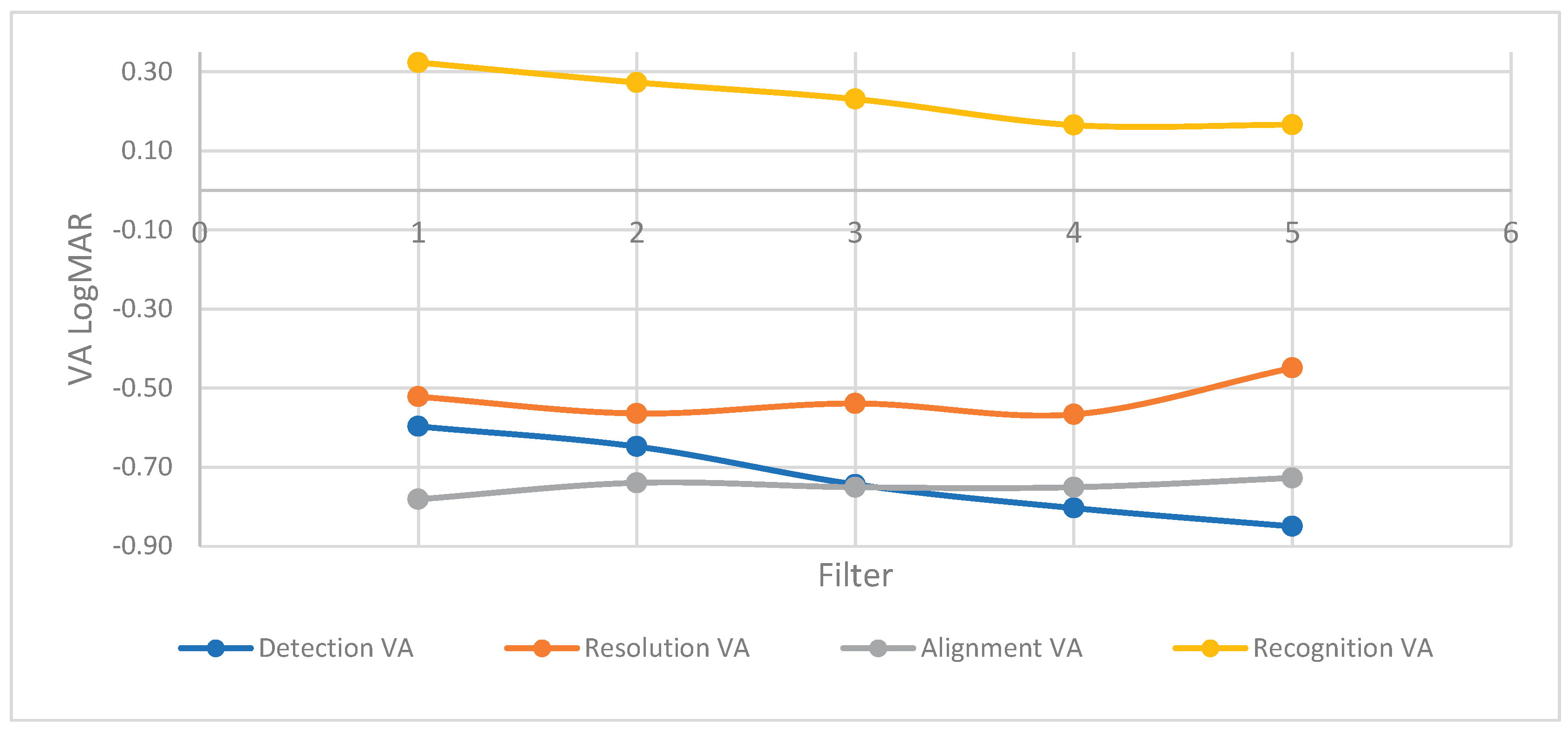
A total of 235 eyes were analyzed. The following mean visual acuity (VA) values were obtained:
Table 9.
Mean Visual Acuity (logMAR) According to Visual Function and Filter Condition.
| Visual Function | Baseline (01) | F1 (02) | F2 (03) | F3 (04) | F4 (05) |
| Detection VA | −0.60 | −0.65 | −0.74 | −0.80 | −0.85 |
| Resolution VA | −0.52 | −0.56 | −0.54 | −0.57 | −0.45 |
| Alignment VA | −0.78 | −0.74 | −0.75 | −0.75 | −0.73 |
| Recognition VA | 0.32 | 0.27 | 0.23 | 0.17 | 0.17 |
Figure 2.
Changes in Visual Acuity (logMAR) Across Filter Conditions for the Four Visual Functions.
Algorithmic Complexity of Visual Acuity Responses
Table 10.
Normalized BDM (nBDM) of Visual Acuity Responses According to Visual Function and Filter Condition.
Table 10.
Normalized BDM (nBDM) of Visual Acuity Responses According to Visual Function and Filter Condition.
| Detection VA | Resolution VA | Alignment VA | Recognition VA | ||||
| nBDM | nBDM | nBDM | nBDM | ||||
| DET01 | 0.8789 | RES01 | 0.8824 | ALI01 | 0.8363 | REC01 | 0.9003 |
| DET02 | 0.8766 | RES02 | 0.8497 | ALI02 | 0.8685 | REC02 | 0.8833 |
| DET03 | 0.8770 | RES03 | 0.8353 | ALI03 | 0.8385 | REC03 | 0.9035 |
| DET04 | 0.8466 | RES04 | 0.8326 | ALI04 | 0.8753 | REC04 | 0.8841 |
| DET05 | 0.8850 | RES05 | 0.8399 | ALI05 | 0.8896 | REC05 | 0.8653 |
Detection Visual Acuity (DET)
The estimated algorithmic complexity of the detection responses remained relatively stable between the baseline condition and DET02–DET03. However, DET04 showed a decrease in nBDM, indicating lower estimated algorithmic complexity of the computational representation of the detection responses under this condition. DET05 subsequently exhibited the highest nBDM value within the detection series.
Given the relatively small differences among the observed values, these findings should be interpreted as preliminary evidence of possible changes in the algorithmic organization of the response representation rather than as conclusive evidence of a systematic effect.
Overall, the filters were associated with non-linear changes in the estimated algorithmic complexity of the detection responses, with a decrease at DET04 followed by an increase at DET05.
Resolution Visual Acuity (RES)
Resolution VA exhibited the clearest decreasing trend in estimated algorithmic complexity. nBDM progressively decreased from the baseline condition (RES01 = 0.8824) to RES04 (0.8326), which represented the minimum value within this series. A slight increase was subsequently observed for RES05 (0.8399).
These findings indicate that the computational representation of the resolution responses became progressively less algorithmically complex up to RES04, followed by a small increase under RES05.
Within the BDM framework used in this study, resolution VA exhibited the clearest pattern of decreasing estimated algorithmic complexity of the computational representation across filter conditions up to RES04, followed by a slight increase in RES05.
Alignment Visual Acuity (ALI)
Alignment responses showed an overall increase in estimated algorithmic complexity across the filter conditions. Although ALI03 exhibited a transient decrease, the nBDM values for ALI04 (0.8753) and ALI05 (0.8896) were higher than the baseline value (0.8363).
This pattern indicates that the computational representation of alignment responses became more algorithmically complex under some filter conditions.
ALI05 exhibited the highest nBDM value within the alignment series.
Recognition Visual Acuity (REC)
Recognition VA exhibited generally high estimated algorithmic complexity across the evaluated conditions. The maximum value was observed for REC03 (nBDM = 0.9035), followed closely by REC01 (nBDM = 0.9003). From REC03 onward, nBDM progressively decreased, reaching 0.8653 at REC05.
This pattern indicates that recognition responses exhibited relatively high algorithmic complexity under the computational representation used in this study, although the filters modified this complexity without a clear monotonic trend.
Among the four visual functions analyzed, recognition included the highest individual nBDM value, observed under REC03.
Global Comparison Across Visual Functions
Considering only the baseline conditions (01):
Table 11.
Comparison of Baseline Normalized BDM (nBDM) Across Visual Functions.
| Visual Function | nBDM |
| Recognition (REC01) | 0.9003 |
| Resolution (RES01) | 0.8824 |
| Detection (DET01) | 0.8789 |
| Alignment (ALI01) | 0.8363 |
The baseline estimated algorithmic complexity followed the order:
This indicates that, even in the absence of filters, the computational representation of the recognition responses exhibited the highest estimated algorithmic complexity, whereas alignment exhibited the lowest value among the visual functions evaluated.
Although some of the observed differences in nBDM values suggest changes in the algorithmic organization of the analyzed representations, the magnitude of these differences was small in some cases. Therefore, these results should be interpreted as evidence consistent with changes in estimated algorithmic complexity rather than as conclusive demonstrations of such changes. Future studies could incorporate bootstrap or other resampling procedures to quantify the statistical stability of BDM estimates.
Because there are currently no universally accepted criteria for establishing thresholds of biologically or computationally relevant differences in nBDM values for computational representations of visual acuity responses, these comparisons should be interpreted primarily from a descriptive and exploratory perspective.
The present study focused on estimating the algorithmic complexity of computational representations of transmittance spectra using BDM. However, this approach represents only an initial application within the broader framework of Algorithmic Information Theory. In particular, more recent developments such as Algorithmic Information Dynamics (AID) extend this framework by investigating how perturbations applied to a system modify its estimated algorithmic complexity and what information these changes may provide about possible underlying generative mechanisms.
In this context, selective optical filters represent an interesting setting for future research. Controlled variations in parameters such as spectral transmittance, bandwidth, material composition, or manufacturing processes could be investigated as perturbations of the system, allowing changes in estimated algorithmic complexity to be evaluated in relation to well-defined physical modifications. This approach could contribute to a deeper understanding of the computational organization of spectral representations and its relationship with observed optical properties.
Likewise, integrating BDM with tools derived from AID, algorithmic perturbation analysis, and causal reconstruction represents a potential direction for the analysis of complex optical data. Although these approaches are beyond the scope of the present study, their future incorporation could extend the characterization of optical systems from the perspective of generative mechanisms, complementing conventional approaches based on statistical measures such as Shannon entropy.
A possible extension of the present work would be to investigate changes in estimated algorithmic complexity during controlled modifications of spectral transmittance, with the aim of identifying regions of stability, transitions in computational organization, or changes consistent with different generative mechanisms. Such an approach would extend the present static characterization of the spectra toward a dynamic analysis of their computational organization.
Comparison with Other Complexity Metrics and Future Perspectives
The present study used BDM as an approximation of algorithmic complexity because this methodology incorporates information related to compressibility and the potential generative mechanisms of computational representations, thereby providing a perspective complementary to conventional statistical measures. Nevertheless, the analysis of complex optical systems could be further enriched by comparison with other metrics widely used in information theory and signal analysis.
Relevant alternatives include Lempel–Ziv complexity, compression-based measures, Approximate Entropy (ApEn), Permutation Entropy (PE), and other computational complexity measures. Each of these approaches characterizes different properties of data organization and may therefore provide complementary information about the computational characteristics of spectral representations.
In particular, whereas Shannon entropy characterizes the statistical uncertainty of a distribution and compression-based measures evaluate redundancy and compressibility within a sequence, BDM approximates algorithmic complexity using CTM-based estimates combined with block decomposition and block multiplicity. These conceptual differences support the use of BDM as the primary algorithmic-complexity estimator in the present study.
Future research could perform comparative analyses to evaluate the sensitivity, discriminatory ability, and complementarity of these metrics when applied to the transmittance spectra of selective optical filters. Such comparisons could more precisely establish the scope and limitations of each methodology and contribute to the development of a more comprehensive framework for the computational characterization of complex optical systems.
In this regard, the contribution of the present study is not to propose BDM as a replacement for other complexity metrics, but rather to demonstrate its feasibility as a complementary tool for the computational analysis of transmittance spectra. Future integration of multiple metrics may provide a more comprehensive and robust characterization of the computational organization of complex optical systems.
General Conclusions
The present study evaluated the algorithmic complexity of transmittance spectra from photoselective filters using the BDM, complemented by Shannon entropy and the assessment of different VA functions. The results demonstrate the feasibility of applying tools derived from Algorithmic Information Theory to characterize the computational organization of optical spectra represented as finite computational objects.
Comparison of Shannon entropy and BDM showed that these metrics characterize different properties of the transmittance spectra. Whereas Shannon entropy quantifies the statistical diversity of the discretized transmittance representation, BDM provides an estimate of its algorithmic complexity. In particular, the behavior observed for F4 showed that greater statistical diversity does not necessarily correspond to greater estimated algorithmic complexity, highlighting the complementary nature of these metrics for spectral characterization.
Analysis of the VA responses revealed differences in nBDM among the visual functions and filter conditions evaluated. However, because some of the observed values were relatively close, these findings should be interpreted cautiously and regarded as preliminary evidence of possible differences in the algorithmic organization of the computational representations of the responses rather than as conclusive evidence of functional effects induced by the filters.
Taken together, the findings are consistent with the hypothesis that BDM provides information complementary to conventional descriptive statistics and Shannon entropy in the analysis of transmittance spectra and computational representations of visual responses. Nevertheless, the conclusions of the present study are restricted to the estimated algorithmic complexity of the representations analyzed and should not be interpreted as measures of the intrinsic physical complexity of the materials or as evidence of causal relationships.
Future studies should incorporate sensitivity analyses addressing discretization and BDM parameter selection, uncertainty estimation using resampling techniques, and comparisons with other complexity and compression metrics. These approaches could provide a more robust assessment of the scope and utility of algorithmic complexity as a complementary tool for investigating photoselective filters and their potential relationship with visual performance.
Overall, the present study provides a proof of concept for the application of algorithmic-complexity methods to the computational characterization of optical spectra and establishes a foundation for future investigations incorporating Algorithmic Information Dynamics (AID). Such approaches may expand the computational analysis of photoselective materials and their associated visual responses.
Author Contributions
Conceptualization, C.A.C.V.; methodology, C.A.C.V.; investigation, C.A.C.V.; data curation, C.A.C.V.; formal analysis, C.A.C.V.; software, C.A.C.V.; visualization, C.A.C.V.; writing—original draft preparation, C.A.C.V.; supervision, A.P.C., I.M.H. and T.S.A. All authors have read and agreed to the published version of the manuscript.
Funding
This research received no external funding.
Informed Consent Statement
Informed consent was obtained from all subjects involved in the study.
Data Availability Statement
The raw data supporting the conclusions of this article will be made available by the authors on request.
Conflicts of Interest
The authors declare no conflicts of interest.
References
- Bonnin Arias, C.; Aguirre Vilacoro, V.; Chamorro Gutiérrez, E.; Sánchez-Ramos, C. Nuevos lentes solares con certificado de seguridad retiniana: Análisis de la función visual mediante la valoración de agudeza visual y estereoscópica, discriminación del color y sensibilidad al contraste. Ciencia y Tecnología para la Salud Visual y Ocular 2015, 13(1), 123–136. [Google Scholar] [CrossRef]
- Capilla, P.; Felipe, A.; Pons, A.; Artigas, J. M. Effect of color on contrast sensitivity with two different accommodative stimuli. Optometry and Vision Science: Official Publication of the American Academy of Optometry 1993, 70(1), 24–29. [Google Scholar] [CrossRef] [PubMed]
- Chaitin, G. J. On the Length of Programs for Computing Finite Binary Sequences: Statistical considerations. Journal of the ACM (JACM) 1969, 16(1), 145–159. [Google Scholar] [CrossRef]
- Cooley, J. W.; Tukey, J. W. An Algorithm for the Machine Calculation of Complex Fourier Series. Mathematics of Computation 1965, 19(90), 297–301. [Google Scholar] [CrossRef]
- Crutchfield, J.; Young, K. Computation at the Onset of Chaos. 1991. Available online: https://www.semanticscholar.org/paper/Computation-at-the-Onset-of-Chaos-Crutchfield-Young/c321c8d9d9231ddfe661a03ae7b872adab3fc3fe.
- Delahaye, J.-P.; Zenil, H. Numerical Evaluation of Algorithmic Complexity for Short Strings: A Glance into the Innermost Structure of Randomness. arXiv 2011, arXiv:1101.4795. [Google Scholar] [CrossRef]
- Guirao Piñera, A. Calidad óptica del ojo humano en función de la edad [Http://purl.org/dc/dcmitype/Text, Universidad de Murcia]. 1999. Available online: https://dialnet.unirioja.es/servlet/tesis?codigo=75787.
- Kolmogorov, A. N. Three approaches to the quantitative definition of information*. International Journal of Computer Mathematics 1968, 2(1–4), 157–168. [Google Scholar] [CrossRef]
- Martín Herranz, R.; Vecilla Antolínez, G. Manual de optometría; Editorial Médica Panamericana, 2011. [Google Scholar]
- Mico, R. M. Optometria Principios Basicos Y Aplicacion Clinica (E. ESPA#A, Ed.); 2011. [Google Scholar]
- Montés-Micó, R. Optometría: Principios básicos y aplicación clínica; Elsevier, 2011. [Google Scholar]
- Rubin, G. S.; Legge, G. E. Psychophysics of reading. VI—The role of contrast in low vision. Vision Research 1989, 29(1), 79–91. [Google Scholar] [CrossRef] [PubMed]
- Shannon, C. E. A Mathematical Theory of Communication. Bell System Technical Journal 1948, 27(3), 379–423. [Google Scholar] [CrossRef]
- Solomonoff, R. J. A formal theory of inductive inference. Part I. Information and Control 1964, 7(1), 1–22. [Google Scholar] [CrossRef]
- Zenil, H.; Badillo, L.; Hernández-Orozco, S.; Hernández-Quiroz, F. Coding-theorem Like Behaviour and Emergence of the Universal Distribution from Resource-bounded Algorithmic Probability. arXiv 2018, arXiv:1711.01711. [Google Scholar] [CrossRef]
- Zenil, H.; Hernández-Orozco, S.; Kiani, N. A.; Soler-Toscano, F.; Rueda-Toicen, A.; Tegnér, J. A Decomposition Method for Global Evaluation of Shannon Entropy and Local Estimations of Algorithmic Complexity. Entropy 2018, 20(8), 605. [Google Scholar] [CrossRef] [PubMed]
- Zenil, H.; Kiani, N. A.; Tegnér, J. Methods of Information Theory and Algorithmic Complexity for Network Biology. arXiv 2015, arXiv:1401.3604. [Google Scholar] [CrossRef]
- Zenil, H.; Kiani, N.; Abrahão, F.; Tegnér, J. Algorithmic Information Dynamics. Scholarpedia 2020, 15(7), 7. [Google Scholar] [CrossRef]
Disclaimer/Publisher’s Note: The statements, opinions and data contained in all publications are solely those of the individual author(s) and contributor(s) and not of MDPI and/or the editor(s). MDPI and/or the editor(s) disclaim responsibility for any injury to people or property resulting from any ideas, methods, instructions or products referred to in the content. |
© 2026 by the authors. Licensee MDPI, Basel, Switzerland. This article is an open access article distributed under the terms and conditions of the Creative Commons Attribution (CC BY) license.
Copyright: This open access article is published under a Creative Commons CC BY 4.0 license, which permit the free download, distribution, and reuse, provided that the author and preprint are cited in any reuse.