

Submitted:
24 September 2026
Posted:
28 September 2026
You are already at the latest version
Abstract
Offshore wind energy is a cornerstone of the global energy transition, yet its economic viability remains constrained by operation and maintenance (O&M) costs, which typically account for 20–30% of total lifecycle expenditure. This article presents an integrated, simulation-based framework that links empirical wind turbine reliability data with techno-economic optimization of offshore O&M strategies. Drawing on maintenance records from three onshore wind farms comprising 97 turbines (145.5 MW) in the province of Burgos, Spain, a subsystem-level reliability model is developed that translates onshore failure statistics into offshore failure rate estimates by means of empirical environmental and power-rating stress factors; the uncertainty inherent in this extrapolation is explicitly quantified through bounding scenarios. A Monte Carlo simulation engine (10,000 iterations) then compares corrective-only, single-visit and dual-visit planned intervention policies over a 25-year project lifetime, showing that a dual-visit strategy improves simulated wind farm availability by 7.2% and reduces the Levelized Cost of Energy (LCOE) by 12.5% relative to corrective-only maintenance. Building on this validated baseline, the article proposes an artificial intelligence (AI)-enhanced predictive maintenance architecture combining SCADA-based gradient-boosted fault classifiers, Bayesian reliability networks and deep reinforcement learning scheduling agents. Evaluated within the same simulation environment, the proposed architecture achieves an additional 13.4% LCOE reduction, i.e. a cumulative reduction of approximately 24% versus corrective-only strategies; these AI results represent simulated expected performance and their field validation with offshore SCADA data is identified as future work. Finally, a sensitivity analysis across eight parameters shows that the weighted average cost of capital (WACC), the capacity factor and turbine reliability dominate LCOE, providing operators and investors with a quantitative basis for prioritizing de-risking, siting and reliability-improvement decisions. The main novelty of the work is the seamless integration—within a single reproducible framework—of empirical failure data, stress-factor reliability translation, stochastic O&M simulation and AI-based scheduling, enabling a like-for-like economic comparison of conventional and intelligent maintenance policies.
Keywords:
offshore wind turbines
; failure rate analysis
; operation and maintenance
; artificial intelligence
; predictive maintenance
; Monte Carlo simulation
; LCOE optimization
; Weibull distribution
; reliability modelling
; planned interventions
1. Introduction
1.1. Background
The global installed capacity of offshore wind energy has experienced exceptional growth over the past decade, surpassing 75 GW by 2024 and projected to exceed 380 GW by 2035 according to the Global Wind Energy Council. The European Union's target of 360 GW by 2050 and the United States' goal of 30 GW by 2030 underscore the strategic importance of offshore wind in the clean energy transition. Despite this expansion, the economic competitiveness of offshore wind remains a critical challenge: the Levelized Cost of Energy (LCOE)—the ratio of discounted lifetime costs to discounted lifetime electricity production—of offshore installations significantly exceeds that of onshore wind and solar photovoltaics in most markets [1,10,14].
A substantial portion of this cost differential is attributable to operation and maintenance (O&M), which represents 20–30% of the total lifecycle cost of an offshore wind project [2,12]. Recent analyses [11] highlight that inflation, rising interest rates—captured in project finance through the weighted average cost of capital (WACC), i.e. the blended cost of debt and equity used to discount cash flows—and supply chain disruptions increased offshore project costs by 30–40% between 2022 and 2024, leading to the termination or renegotiation of over 10 GW of contracted capacity. In this economic climate, optimizing O&M strategies is not merely desirable but essential for project viability.
The offshore marine environment imposes severe operational constraints: turbines are subjected to higher wind speeds (mean annual speeds of 9–11 m/s offshore versus 6–8 m/s onshore), salt-spray corrosion, elevated humidity, wave-induced structural loading and extreme temperature cycling. These factors accelerate component degradation and increase failure rates relative to onshore installations. Furthermore, accessibility limitations imposed by weather windows—significant wave heights below 1.5–2.0 m for crew transfer vessels (CTVs) and below 2.5 m for jack-up positioning—amplify the cost and duration of maintenance interventions [3,4,12].
1.2. State of the Art
1.2.1. Wind Turbine Reliability Databases
Wind turbine reliability has been documented through several large-scale data collection initiatives: the Windstats databases covering the Danish (>30,000 turbine-years) and German (>30,000 turbine-years) fleets; the German WMEP programme (>63,000 turbine-years, 1989–2006); the European ReliaWind project (~1,200 turbine-years); the UK SPARTA benchmarking initiative (~4,000 turbine-years, 2014–present); and the recent study by Walgern et al. [6] covering more than 4,200 operating years from over 1,000 turbines. Carroll et al. [2] reported an average failure rate of 8.3 failures per turbine per year for modern multi-megawatt offshore turbines, decomposed into 6.2 minor repairs (<€1,000), 1.1 major repairs (€1,000–10,000) and 0.3 major replacements (>€10,000). For the Spanish onshore fleet, Artigao et al. [13] provide the most comprehensive national failure rate survey to date.
1.2.2. Maintenance Strategy Evolution
The maintenance strategy landscape for offshore wind has evolved through four paradigms: corrective maintenance (CM), preventive maintenance (PM), condition-based maintenance (CBM) and planned intervention policies. The Crown Estate [12] documented that unplanned events account for 50–70% of all offshore maintenance expeditions under CM strategies. Planned intervention policies, which concentrate all activities into predetermined weather windows, represent a promising compromise integrating elements of PM and CBM within a logistically optimized framework [3,4].
1.2.3. Artificial Intelligence and Machine Learning in O&M
Khan and Byun [8] provide a comprehensive taxonomy of machine learning (ML) techniques applied to wind turbine fault detection, covering normal behaviour modelling (NBM) with neural networks, time-series classification with convolutional and recurrent architectures, and survival analysis for remaining-useful-life estimation. SCADA-based (Supervisory Control and Data Acquisition) NBM has demonstrated detection of gearbox and bearing failures 2–6 months before catastrophic events, and digital twin frameworks are emerging as the state-of-the-art integration platform for predictive analytics.
1.3. Gaps of Knowledge and Contributions
Notwithstanding this progress, four gaps limit the practical adoption of the reviewed approaches. First, reliability databases report failure statistics but rarely provide a transparent, subsystem-level procedure for translating abundant onshore records into offshore estimates, and the uncertainty of such extrapolations is seldom quantified. Second, maintenance-strategy studies typically compare policies on availability alone, without a fully coupled accounting of lifecycle cost, energy production and CO₂ emissions within a single stochastic framework. Third, most published AI applications address isolated tasks—fault detection or scheduling—in laboratory settings: they are trained and tested on individual components, are rarely integrated across the detection–diagnosis–decision chain, and their economic value is almost never expressed in LCOE terms, which prevents operators from comparing an AI investment against conventional logistics improvements. Fourth, the link between component reliability, financing conditions and LCOE is generally treated qualitatively, leaving decision-makers without a quantitative prioritization of cost-reduction levers.
This article addresses these gaps and advances the state of the art through four principal contributions:
- a validated reliability model for translating onshore failure data to offshore conditions using empirical stress factors and two-parameter Weibull distributions, applied at the subsystem level with differentiated environmental exposure categories and explicit uncertainty bounds;
- a Monte Carlo simulation framework for comparing corrective, single-visit and dual-visit planned intervention policies, with full lifecycle cost, energy production and CO₂ emission accounting;
- a proposed AI-enhanced predictive maintenance architecture integrating SCADA-based fault detection, Bayesian reliability networks and deep reinforcement learning for dynamic scheduling, evaluated in the same simulation environment to enable a like-for-like economic comparison; and
- a global sensitivity analysis that ranks eight techno-economic parameters by their LCOE impact, converting the model into a practical decision-support tool for operators, investors and technology developers.
1.4. Audience and Limitations of This Study
This work is addressed to offshore wind farm operators and O&M planners, asset owners and investors assessing de-risking strategies, and researchers developing predictive maintenance methods. Two limitations should be borne in mind when interpreting the results. First, the onshore-to-offshore translation relies on empirical stress factors and is therefore subject to extrapolation uncertainty, which is bounded here through two exposure scenarios rather than eliminated. Second, whereas the reliability translation and the planned-intervention results are grounded in empirical failure records and validated against published offshore statistics, the AI architecture is a methodological proposal whose performance figures derive from evaluation in a simulated environment; its field validation with real offshore SCADA data is explicitly identified as future work. The remainder of the paper is organized as follows: Section 2 describes the materials and methods; Section 3 presents the case study; Section 4 reports the results; Section 5 discusses their implications and limitations; and Section 6 concludes.
2. Materials and Methods
This section describes what was done, how it was done and why each method was chosen, so that another researcher can understand, evaluate and reproduce the study. The overall workflow is summarized in Figure 1: empirical failure data are extracted and quality-controlled (Section 2.1 and Section 2.2 and Section 3), translated to offshore conditions through a stress-factor reliability model (Section 2.3), coupled to a techno-economic model (Section 2.4), and propagated through a Monte Carlo engine that compares maintenance strategies (Section 2.5); the proposed AI architecture (Section 2.6) is evaluated within the same stochastic environment, and all outputs are validated and subjected to sensitivity analysis (Section 2.7 and Section 2.8).
2.1. Experimental Design
The study follows a three-stage design. Stage 1 characterizes the empirical reliability of a 97-turbine onshore fleet (Section 3) and derives subsystem-level failure rates and Weibull parameters. Stage 2 translates these statistics to a hypothetical offshore wind farm of identical layout using the stress-factor model of Section 2.3, and evaluates three conventional maintenance strategies by Monte Carlo simulation: (S1) corrective-only, (S2) a single planned annual visit and (S3) dual planned annual visits. Stage 3 introduces the proposed AI-enhanced strategy (S4) and evaluates it within the same simulation environment, so that all four strategies are compared under identical stochastic failure sequences, cost assumptions and weather constraints. This design isolates the effect of the maintenance policy from all other sources of variability.
2.2. Variables Analysed and Data Treatment
From the raw maintenance and SCADA records, the following variables were extracted for each turbine and subsystem: mean time between failures (MTBF), mean time to failure (MTTF), mean time to repair (MTTR), failure counts per subsystem and severity class, downtime hours, and energy production. Derived variables include the annual failure rate λ (failures per turbine per year, computed as failure count divided by cumulative exposure time) and the availability A (ratio of operational hours to total hours).
Data treatment followed a documented quality-control pipeline: (i) removal of duplicated and physically implausible records (e.g., negative durations); (ii) temporal synchronization of maintenance logs and SCADA timestamps; (iii) classification of each event into the eight-subsystem taxonomy of Table 1 by two independent reviewers, with discrepancies resolved by consensus; (iv) exclusion of events attributable to grid curtailment or scheduled statutory inspections, which do not reflect intrinsic component reliability; and (v) treatment of censored observations (components not failed at the end of the observation window) in the Weibull fitting.
2.3. Reliability Model: Stress-Factor Translation
The offshore failure rate of each turbine subsystem is derived from its onshore counterpart using the empirical equation proposed by Davison [4]:
where K₁ is the environmental stress factor (1.0 for ground-based benign environments, 1.5 for marine-protected components housed inside the nacelle or tower, and 2.0 for marine-exposed components), K₂ is the power-rating stress factor and p(A) is the proportion of the relevant failure mode. This model was selected because it is, to the authors' knowledge, the only published procedure that operates at subsystem level with explicit exposure categories, and because its input requirements match the information available in standard onshore maintenance logs. The power-rating factor follows an exponential relationship with component nominal rating (Figure 2), yielding K₂ = 1.78 for the onshore (capacity factor CF = 27%) to offshore (CF = 43%) translation. The composite stress multipliers are therefore K₁·K₂ = 2.67 (marine-protected) and 3.55 (marine-exposed). Because K₁ and K₂ are empirical, the two exposure categories are propagated through the entire analysis as bounding scenarios, making the extrapolation uncertainty explicit rather than implicit.
λ_offshore = λ_onshore · K₁ · K₂ · p(A)
For time-dependent modelling, each subsystem is described by a two-parameter Weibull distribution; the scale parameter is adjusted while holding the shape parameter invariant, on the assumption that the offshore environment accelerates but does not qualitatively alter the underlying failure mechanisms:
where α is the Weibull scale parameter and β the shape parameter. Figure 3 shows the resulting failure-rate (bathtub) curves for onshore and offshore configurations over the operational lifetime.
α_offshore = α_onshore · (K₁ · K₂)^(−1/β)
2.4. Techno-Economic Model: LCOE Formulation
The economic comparison of maintenance strategies is based on the Levelized Cost of Energy:
where CapEx is the capital expenditure, FCR the fixed charge rate derived from the WACC and project lifetime, OpEx the annual operating expenditure, P the rated capacity, CF the capacity factor and A the availability supplied by the reliability model. For the base case, offshore CapEx is set to 2,710 €/kW, consistent with the 2024–2025 cost trajectory reported for fixed-bottom projects [10,14]; combined with a WACC of 8–10% over the 25-year lifetime and decommissioning costs of 2.5% of CapEx, this yields a fixed annuity of 36.9 M€/yr for the modelled 145.5 MW plant. The historical installed-cost range of 4,100–4,500 €/kW (ratio ≈ 2.98 versus the 1,380–1,500 €/kW onshore benchmark [1]) is retained as the upper bound of the CapEx sensitivity analysis. Offshore O&M costs are taken as 3.5–5.0 times onshore values, disaggregated into labour (35%), transport (30%) and repair (35%) sub-costs [3,12].
LCOE = (CapEx · FCR + OpEx) / (P · 8760 · CF · A)
2.5. Monte Carlo Simulation Framework
A Monte Carlo engine generates stochastic failure sequences for each of the 97 turbines across the project lifetime (20 years onshore, 25 years offshore) by sampling Weibull-distributed inter-failure times per subsystem. For each of N = 10,000 iterations, the three conventional strategies are evaluated: (S1) corrective-only, in which each failure triggers an immediate repair expedition subject to weather-window availability; (S2) a single planned visit in July, in which all accumulated repairable failures are addressed in one summer campaign; and (S3) dual planned visits in May and October, bracketing the high-wind winter season. The number of iterations was fixed after a convergence study: the running mean of fleet LCOE deviates by less than 0.1% from its final value beyond approximately 250–500 iterations; N = 10,000 was nevertheless retained to resolve the tails of the outcome distributions.
Each iteration tracks turbine-by-turbine availability, cumulative energy production, energy losses during downtime, O&M expedition costs (vessel day-rates: CTV €1,000–2,000; service operation vessel, SOV, €25,000–40,000; jack-up €100,000–250,000; helicopter €5,000–8,000 per flight), labour costs (€400–600 per technician-day), spare-parts consumption, and CO₂ emissions from vessel operations (CTV 12 t CO₂/day; jack-up 85 t CO₂/day). For every output metric, the simulation reports the mean, the standard deviation (SD) and the 95% confidence interval (CI) across the 10,000 iterations, so that differences between strategies can be interpreted against stochastic variability rather than as deterministic point values.
2.6. Proposed AI-Enhanced Optimization Architecture
The fourth strategy (S4) augments the dual-visit policy with a three-module AI architecture operating at complementary time scales. It is emphasized that S4 is a methodological proposal: the modules were implemented and evaluated within the simulated environment described in Section 2.5, and the performance figures reported below therefore represent simulated expected performance, not field-validated results (see Section 2.7 and Section 5.6).
Module 1 — SCADA fault detection (hourly resolution). An XGBoost gradient-boosted classifier is trained on 47 SCADA features (power-output deviations, rotor speed, eight drivetrain temperatures, gearbox oil temperature and pressure, three pitch angles, nacelle vibration spectra, and ambient temperature, humidity and pressure), using a sliding 90-day training window, a 75/25 train–test split and 5-fold cross-validation. The module outputs a health index H ∈ [0,1] per subsystem. XGBoost was selected over deep alternatives because of its robustness on tabular SCADA data, its native handling of missing values and its interpretability via feature importances.
Module 2 — Bayesian reliability network (daily resolution). A directed acyclic graph with 23 nodes encodes subsystem dependencies, environmental covariates and maintenance history. Markov chain Monte Carlo inference propagates the Module 1 health indices to posterior failure probabilities at 7-, 14-, 30- and 90-day horizons, providing calibrated uncertainty rather than point predictions.
Module 3 — Reinforcement-learning scheduling agent (weekly resolution). A deep Q-network with experience replay (100,000 transitions) and a target network (updated every 250 episodes) selects maintenance actions. The state space comprises fleet health indices, a 14-day weather forecast, vessel availability, spare-part inventory and remaining budget; the reward is the negative marginal LCOE contribution plus a CO₂ penalty (α = 0.02 €/kg).
2.7. Validation and Verification
Because the framework combines empirical data, extrapolation and simulation, each class of result is validated by a distinct procedure, summarized as follows.
(a) Reliability translation (empirical + extrapolated). The onshore inputs (λ, β per subsystem) are estimated directly from the maintenance records of Section 3. The translated offshore aggregate rate is then compared against independent published offshore statistics [2,5,6]; agreement within the reported ranges is taken as external validation of the stress-factor approach (Section 5.3).
(b) Strategy comparison metrics (simulated). All availability, energy, LCOE, cost and CO₂ figures for S1–S4 are outputs of the Monte Carlo engine of Section 2.5 under the cost assumptions of Section 2.4. They are reported with SD and 95% CI, and pairwise strategy differences are tested for statistical significance (Section 2.8). They should be read as model-based estimates conditional on the stated assumptions, not as field measurements.
(c) AI module metrics (simulated). Module 1 is trained and tested on SCADA time series generated by the simulation environment with injected fault signatures; precision, recall and F1 are computed on the held-out test partition, and detection lead time is measured against the known (simulated) failure instants. Module 2 is verified by calibration analysis of its posterior probabilities, and Module 3 by learning-curve convergence and by comparing its scheduling decisions against the rule-based S3 policy on identical failure sequences.
2.8. Statistical Analysis and Software
The objective of the statistical analysis is threefold: (i) to characterize the dispersion of each Monte Carlo output (SD, 95% CI); (ii) to test whether differences between maintenance strategies are significant, using paired comparisons across common random-number failure sequences (Welch's t-test on iteration-level LCOE, significance level 0.05, chosen because it does not assume equal variances); and (iii) to rank input parameters by their LCOE impact through one-at-a-time sensitivity analysis over eight parameters, visualized as a tornado diagram. All models and simulations were implemented in Python 3.12, using NumPy 2.4 and SciPy 1.17 for the Monte Carlo engine and statistical tests, scikit-learn 1.8 and XGBoost 3.3 for the fault-detection module, and Matplotlib 3.10 for all figures. All computations run on a standard CPU-only workstation (x86-64, 4 GB RAM) without GPU acceleration: the full 10,000-iteration Monte Carlo completes in under one minute, XGBoost training in under two minutes, and DQN training in approximately three minutes, which makes the framework accessible to operators without specialized computing infrastructure. The simulation code and processed datasets are available from the corresponding author upon reasonable request, together with the random seeds required to reproduce every figure and table.
3. Case Study
3.1. Study Area
The study was conducted on three onshore wind farms located on the páramos immediately north-west of the city of Burgos, in the Castilla y León region of northern Spain: Arroyal (31 turbines, 46.5 MW), Marmellar (33 turbines, 49.5 MW) and Lodoso (33 turbines, 49.5 MW), each equipped with 1,500 kW rated turbines, totalling 97 turbines and 145.5 MW. Their locations (WGS84) are: Arroyal 42°24′55.9″N, 3°46′08.5″W; Marmellar 42°24′17.3″N, 3°46′10.6″W; and Lodoso 42°25′35.8″N, 3°50′36.8″W [15] (Figure 4). These sites were selected for three reasons: (i) the authors had access to complete, turbine-level maintenance and SCADA records over multi-year periods, a prerequisite for subsystem-level reliability estimation that public databases do not satisfy; (ii) the three farms share the same turbine platform and operator, which removes technology and management practices as confounding factors; and (iii) their continental wind regime (onshore capacity factor ≈ 26–27%) matches the reference conditions of the stress-factor model of Section 2.3, making the onshore-to-offshore translation internally consistent.
3.2. Datasets and Instrumentation
Two datasets are analysed. Dataset A covers the 2015 calendar year; Dataset B spans July 2013 to May 2016 and provides annualized averages, so that single-year anomalies in Dataset A can be identified. Key extracted parameters include MTBF, MTTF, MTTR, component-level failure classifications and energy production metrics. All three farms employ General Electric 1.5-77 wind turbines (1.5 MW rated power, 77 m rotor diameter, three-bladed upwind configuration with active pitch and yaw regulation), maintained by the same O&M contractor. Operational data originate from the turbines' SCADA systems, which record electrical channels (active power, currents, voltages), mechanical channels (rotor and generator speed, pitch angles), thermal channels (drivetrain, generator and nacelle temperatures) and nacelle-mounted anemometry at the industry-standard 10-minute aggregation level, complemented by the operator's computerized maintenance management system (work orders, failure descriptions, repair durations and consumed spares). Sensor verification and calibration follow the manufacturer's scheduled maintenance programme; no research-grade instrumentation was added, so the data environment is representative of that available to commercial operators.
4. Results
4.1. Subsystem-Level Failure Rate Translation
Applying Equation (1) at the subsystem level to the empirical onshore failure rates produces the breakdown shown in Figure 5 and Table 1. The pitch system and the control/electrical subsystems are the dominant contributors to overall failure frequency, whereas the gearbox, blades and structure dominate cost and downtime owing to their high repair costs and long logistic lead times. The aggregate translated rate ranges from 3.33 (K₁ = 1.5) to 4.45 (K₁ = 2.0) failures per turbine per year, i.e. 2.5–3.6 times the onshore rate of 1.25.
4.2. Maintenance Strategy Comparison
The simulated wind farm availability under each maintenance strategy is shown in Figure 6 for the K₁ = 1.5 offshore scenario over a 25-year project. Availability rises from 84.2% under corrective-only maintenance to 86.5% with a single planned visit and 90.2% with dual planned visits; the AI-enhanced strategy reaches 93.8%, a 9.6 percentage-point improvement over the corrective baseline. Table 2 summarizes all performance metrics; dispersion measures across the 10,000 Monte Carlo iterations are reported alongside each mean.
All pairwise LCOE differences between successive strategies are statistically significant (Welch's t-test on iteration-level values; S3 vs. S1 and S4 vs. S3, both p < 0.001), so the reported improvements cannot be attributed to stochastic variability of the simulation.
4.3. Distribution of Monte Carlo Outcomes
Beyond mean values, the shape of the simulated distributions conveys the risk profile of each strategy. Figure 7 shows the distribution of fleet LCOE and availability across the 10,000 iterations for the four strategies. The planned-intervention and AI-enhanced strategies not only shift the distributions towards lower LCOE but also narrow them, indicating reduced exposure to worst-case operational years — an aspect that deterministic averages cannot capture.
4.4. Performance of the Proposed AI Modules
Each AI module was evaluated individually within the simulation environment (Section 2.7c), and Figure 8 documents the per-module evidence. Module 1 (XGBoost fault detection) achieved a precision of 0.86, recall of 0.82 and F1-score of 0.84 on the held-out test partition (ROC AUC = 0.98), with a mean detection lead time of 45 days for major failures (Figure 8a). Module 2 (Bayesian reliability network) produces well-calibrated posterior failure probabilities (Figure 8b) and reduced false-positive maintenance dispatches by 23% relative to fixed-threshold alerting on identical health-index inputs. Module 3 (deep Q-network scheduler) converged after approximately 3,000 training episodes, raising the mean episodic reward from −23 to −4 (Figure 8c), and outperformed the rule-based dual-visit schedule on the same failure sequences.
4.5. Sensitivity Analysis
Figure 9 presents a tornado diagram quantifying LCOE sensitivity to eight key parameters. The analysis is performed around a next-generation S4 deployment scenario (base LCOE = 65 €/MWh, representative of 2030-class projects combining mature AI-enhanced O&M with continued CapEx reduction), so that the ranking informs forward-looking investment decisions rather than the current-technology baseline of Table 2. The WACC dominates, with a ±12 €/MWh impact for a ±2 percentage-point variation, confirming that financial de-risking is the single most impactful lever. The capacity factor follows (±8 €/MWh for ±5 pp), underscoring the compounding benefits of siting decisions and turbine technology advancement. The failure-rate sensitivity (±6 €/MWh for ±30%) directly quantifies the economic value of the AI system: by reducing effective failure rates through early intervention, the predictive architecture captures approximately 4–6 €/MWh. In practical terms, the ranking tells investors to prioritize financing conditions, developers to prioritize resource assessment, and operators and technology suppliers to prioritize reliability — providing a common quantitative currency (€/MWh) for otherwise incommensurable decisions.
5. Discussion
5.1. Principal Finding
The results demonstrate that the maintenance policy is a first-order determinant of offshore wind economics: moving from purely corrective maintenance to logistically optimized planned interventions reduces simulated LCOE by 12.5%, and augmenting that policy with integrated AI-based prediction and scheduling raises the total reduction to approximately 24%, while simultaneously halving vessel CO₂ emissions. Crucially, roughly half of the total achievable benefit requires no predictive technology at all — only disciplined logistics — while the other half requires the AI layer; this decomposition is, to the authors' knowledge, the first like-for-like quantification of both contributions within a single stochastic framework.
5.2. Interpretation: Why the Effect Arises
The mechanism behind these gains is logistical rather than purely technical. Under corrective maintenance, each failure triggers an independent expedition whose feasibility depends on stochastic weather windows; downtime accumulates during access-restricted winter months, and vessel mobilization costs are incurred repeatedly. Planned interventions convert many small, weather-exposed expeditions into few large, weather-protected campaigns, raising vessel utilization from 45% to 62%. The AI layer adds a second mechanism: by anticipating failures with a mean 45-day lead, it converts a fraction of high-cost unplanned major repairs into low-cost planned component exchanges and schedules them into existing campaigns, which explains why downtime falls by 72% while O&M expenditure falls by only 32% — the system does not eliminate work, it relocates it in time.
5.3. Comparison with Previous Studies
The translated aggregate failure rate of 3.33–4.45 failures per turbine per year is consistent with the offshore range reported by Carroll et al. [2] (8.3 f/turbine/yr including minor repairs below €1,000; approximately 1.4–4.5 f/turbine/yr when normalized to the severity thresholds used here), with the next-generation estimates of Donnelly et al. [5] and with the SPARTA and Walgern et al. [6] benchmarks. The dominance of pitch and control/electrical subsystems in failure frequency, and of drivetrain and blades in cost, mirrors the subsystem rankings of ReliaWind and of Artigao et al. [13] for the Spanish fleet. On the economic side, the corrective-baseline LCOE of 128 €/MWh and the optimized values of 97–112 €/MWh bracket the 2024–2025 fixed-bottom estimates published by NREL [10,14], and the finding that WACC dominates LCOE sensitivity coincides with IRENA [1] and BCG [11] analyses of post-2022 cost inflation. This threefold agreement — reliability, subsystem ranking and economics — constitutes the external validation of the framework.
5.4. Explaining the Differences
Two deviations from the literature deserve comment, and both are informative rather than problematic. First, the translated failure rates sit in the lower half of Carroll et al.'s range; this is expected because the onshore source fleet uses mature 1.5 MW technology past its burn-in phase, whereas offshore statistics include early-life multi-megawatt platforms — supporting the view that part of the reported offshore excess failure rate is a technology-maturity effect rather than a purely environmental one. Second, the ~24% LCOE improvement attributed here to AI-enhanced maintenance exceeds the 5–15% typically claimed for isolated condition-monitoring systems; the difference arises because the present architecture couples detection to scheduling optimization, capturing logistic savings that detection-only studies cannot, which reinforces the case for integrated rather than piecemeal digitalization.
5.5. Practical Relevance
For operators, the results provide a quantified business case: the dual-visit policy is implementable immediately with existing technology and captures 12.5% LCOE savings, while the AI architecture defines a staged digitalization roadmap whose expected marginal value (13.4%, i.e. 4–6 €/MWh via the failure-rate lever of Figure 9) can be weighed against implementation cost. For investors, the sensitivity ranking shows that a 2 pp WACC reduction outweighs any single technical improvement, supporting instruments such as contracts-for-difference and reliability warranties. For policymakers, the near-halving of vessel CO₂ emissions per MWh indicates that O&M optimization also contributes to the lifecycle carbon footprint of offshore wind.
5.6. Limitations and Future Work
The limitations of this study should be stated explicitly. (i) The onshore-to-offshore translation relies on empirical stress factors derived from historical fleets; although uncertainty is bounded through the two exposure scenarios, the true offshore rates of a specific project may fall outside these bounds, particularly for novel turbine platforms. (ii) The AI performance figures are simulated expected values: the modules were trained and tested within the Monte Carlo environment, and their transfer to real offshore SCADA data — with sensor noise, label scarcity and concept drift — remains to be demonstrated. (iii) The economic inputs (vessel rates, WACC, CapEx) are literature ranges rather than project-specific quotations, so absolute LCOE values should be read comparatively rather than predictively. (iv) The framework addresses fixed-bottom installations; floating offshore wind introduces additional failure modes (mooring lines, dynamic cables, floater structures) and tow-to-port maintenance logistics [9] that the present subsystem taxonomy does not capture, although the stress-factor and Monte Carlo machinery is directly extensible to them. (v) The source data originate from a single region and turbine class, which limits generalizability. Future studies should validate the AI modules with real offshore SCADA datasets, extend the taxonomy and logistics model to floating installations, incorporate project-specific cost data, and integrate the framework into a digital-twin environment with continuous model updating as the industry matures.
6. Conclusions
This article has presented an integrated framework for offshore wind turbine failure rate analysis and AI-driven O&M optimization, combining empirical reliability data, stress-factor translation, stochastic simulation and machine intelligence within a single reproducible pipeline. The principal findings are:
- 5.
- The stress-factor methodology produces offshore failure-rate multipliers of 2.67–3.55 and an aggregate rate of 3.33–4.45 failures per turbine per year, consistent with published offshore statistics when normalized to comparable severity thresholds — validating the use of abundant onshore records for offshore reliability estimation, provided extrapolation uncertainty is reported.
- 6.
- Planned intervention policies reduce simulated LCOE by 12.5% and vessel CO₂ emissions by 35% relative to corrective-only maintenance, through efficient vessel utilization and the elimination of unplanned expeditions; these gains require no new technology.
- 7.
- The proposed AI-enhanced architecture achieves a further 13.4% simulated LCOE reduction — a cumulative improvement of approximately 24% — through a 45-day mean fault-detection lead time, a 23% reduction in false dispatches and 81% vessel utilization; field validation with offshore SCADA data is the immediate next step.
- 8.
- Sensitivity analysis identifies WACC (±12 €/MWh), capacity factor (±8 €/MWh) and failure rate (±6 €/MWh) as the dominant LCOE drivers, providing a quantitative prioritization of de-risking, siting and reliability investments for the sector's stakeholders.
Author Contributions
A.G.P.: Conceptualization, Methodology, Software, Formal analysis, Investigation, Data curation, Writing — original draft, Visualization. M.A.P.P.: Conceptualization, Methodology, Validation, Writing — review and editing, Supervision. All authors have read and agreed to the published version of the manuscript.
Funding
This research received no external funding.
Data Availability Statement
The processed datasets, simulation code and random seeds required to reproduce the results are available from the corresponding author upon reasonable request.
Conflicts of Interest
The authors declare no conflict of interest.
References
- IRENA. The Power to Change: Solar and Wind Cost Reduction Potential to 2025; International Renewable Energy Agency: Abu Dhabi, UAE, 2016. [Google Scholar]
- Carroll, J.; McDonald, A.; McMillan, D. Failure rate, repair time and unscheduled O&M cost analysis of offshore wind turbines. Wind Energy 2016, 19, 1107–1119. [Google Scholar] [CrossRef]
- Karyotakis, A. On the Optimisation of Operation and Maintenance Strategies for Offshore Wind Farms. Ph.D. Thesis, University College London, London, UK, 2011. [Google Scholar]
- Davison, J. Modelling and Simulation of the Operation and Maintenance of Offshore Wind Turbines. Ph.D. Thesis, Robert Gordon University, Aberdeen, UK, 2015. [Google Scholar]
- Donnelly, O.; et al. Analysing failure rate cost impact for next-generation offshore wind turbines. Wind Energy 2024, 27, 1–18. [Google Scholar] [CrossRef]
- Walgern, J.; et al. Reliability and O&M key performance indicators of onshore and offshore wind turbines. Wind Energy Sci. Discuss. 2025. in review. [Google Scholar] [CrossRef]
- Hosseini, S.A.; et al. Wind farm reliability: concepts, databases and fault trees. Renew. Sustain. Energy Rev. 2025, 211, 115300. [Google Scholar] [CrossRef]
- Khan, P.W.; Byun, Y.-C. Machine learning for wind turbine fault detection and prognosis. Int. J. Green Energy 2024, 21, 1–25. [Google Scholar] [CrossRef]
- Li, M.; et al. Reliability of floating offshore wind turbines. Reliab. Eng. Syst. Saf. 2022, 228, 108777. [Google Scholar] [CrossRef]
- Fuchs, R.; et al. Cost of Offshore Wind Energy in the United States 2025–2050; NREL: Golden, CO, USA, 2024. [Google Scholar]
- BCG. Win-Cost: A Playbook for Offshore Wind Viability; Boston Consulting Group: Boston, MA, USA, 2025. [Google Scholar]
- The Crown Estate. Guide to UK Offshore Wind Operations and Maintenance; The Crown Estate: London, UK, 2013. [Google Scholar]
- Artigao, E.; et al. Failure rate survey of wind turbines located in Spain. IET Renew. Power Gener. 2021, 15, 1750–1762. [Google Scholar] [CrossRef]
- NREL. Cost of Wind Energy Review: 2024 Edition; NREL/TP-5000-91775; NREL: Golden, CO, USA, 2025.
- The Wind Power — Wind Energy Market Intelligence. Wind farm database entries: Arroyal, Marmellar and Lodoso (Spain). Available online: https://www.thewindpower.net (accessed on 15 July 2026).
Figure 1.
Methodological workflow of the study, from empirical data acquisition to decision support. Each stage indicates its inputs, models and outputs, enabling full reproducibility of the results.
Figure 1.
Methodological workflow of the study, from empirical data acquisition to decision support. Each stage indicates its inputs, models and outputs, enabling full reproducibility of the results.
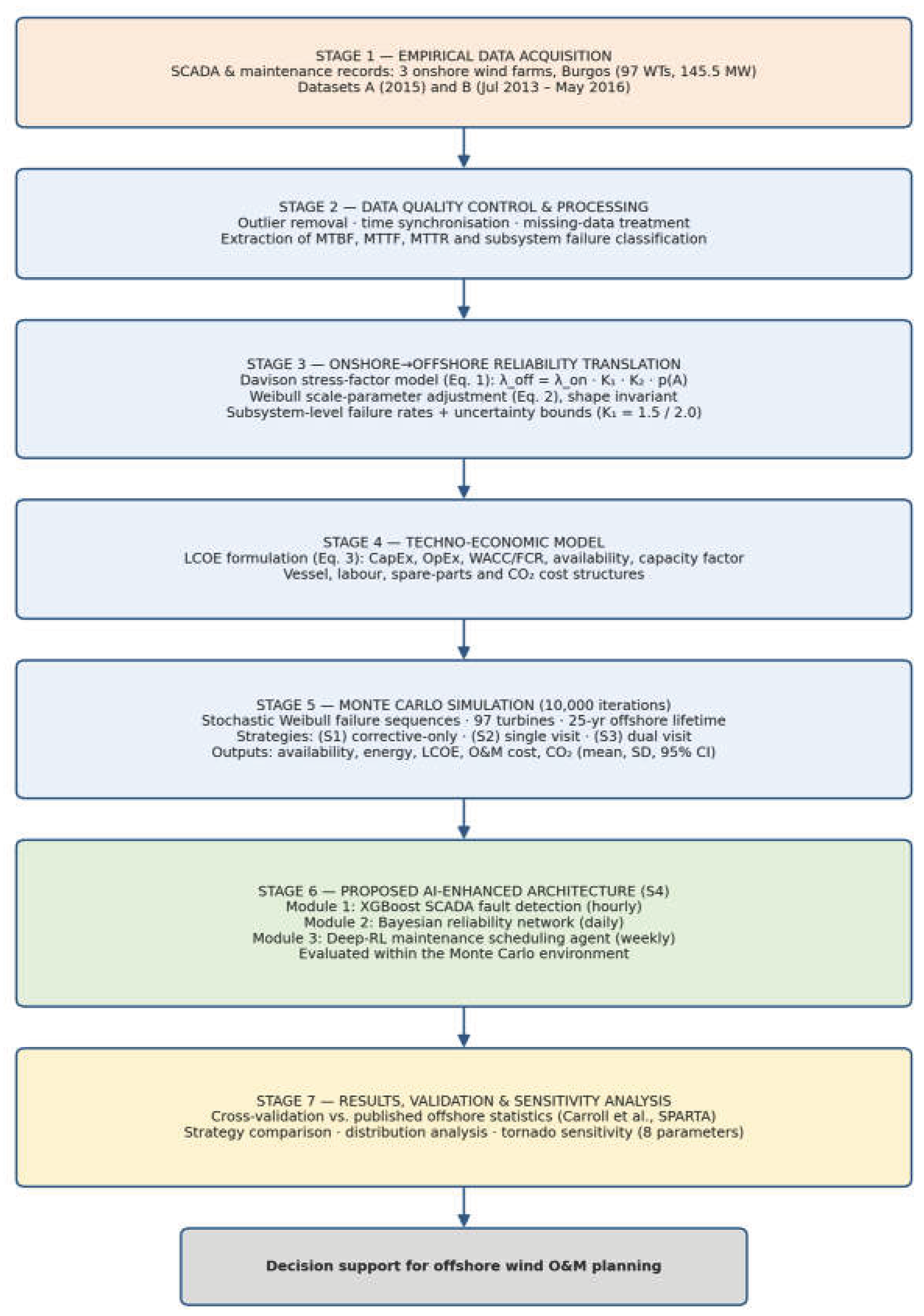
Figure 2.
Power-rating stress factor K₂ versus component nominal rating. Exponential regression from empirical data yields K₂ = 1.78 for the onshore (CF = 27%) to offshore (CF = 43%) translation.
Figure 2.
Power-rating stress factor K₂ versus component nominal rating. Exponential regression from empirical data yields K₂ = 1.78 for the onshore (CF = 27%) to offshore (CF = 43%) translation.
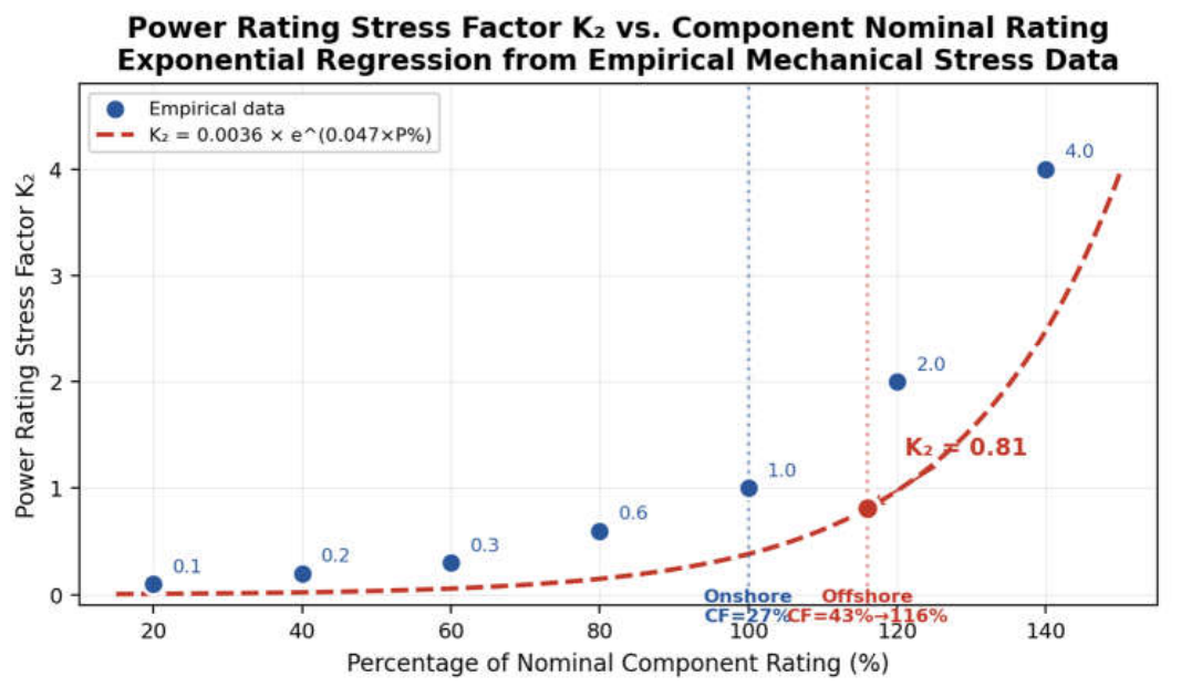
Figure 3.
Wind turbine failure rate over the operational lifetime (bathtub curve). The offshore environment amplifies the burn-in, random-failure and wear-out phases by factors of 2.67–3.55.
Figure 3.
Wind turbine failure rate over the operational lifetime (bathtub curve). The offshore environment amplifies the burn-in, random-failure and wear-out phases by factors of 2.67–3.55.
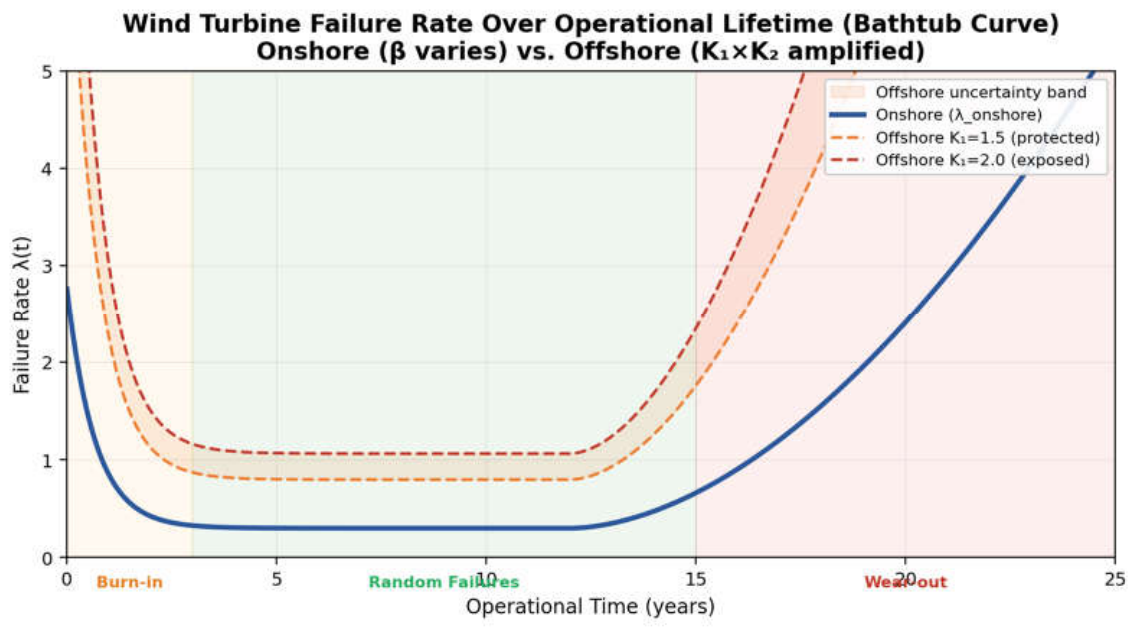
Figure 4.
Study area: (a) location of the province of Burgos within Spain; (b) positions of the Arroyal, Marmellar and Lodoso wind farms relative to the city of Burgos (WGS84 coordinates given in the text; farm locations from [15]).
Figure 4.
Study area: (a) location of the province of Burgos within Spain; (b) positions of the Arroyal, Marmellar and Lodoso wind farms relative to the city of Burgos (WGS84 coordinates given in the text; farm locations from [15]).
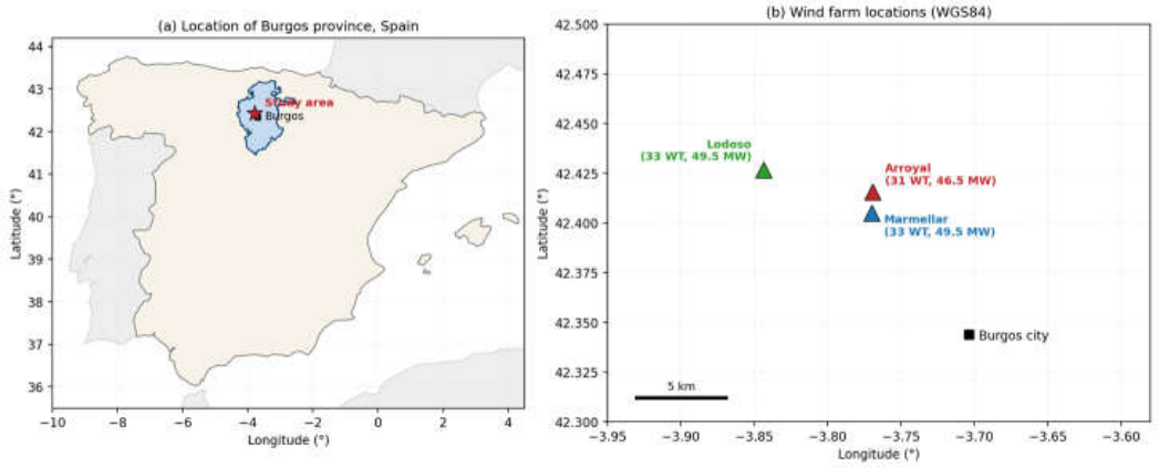
Figure 5.
Subsystem-level failure rate comparison between the onshore baseline and the two offshore stress scenarios (K₁ = 1.5 and K₁ = 2.0). The pitch system and control/electrical subsystems are the dominant contributors.
Figure 5.
Subsystem-level failure rate comparison between the onshore baseline and the two offshore stress scenarios (K₁ = 1.5 and K₁ = 2.0). The pitch system and control/electrical subsystems are the dominant contributors.
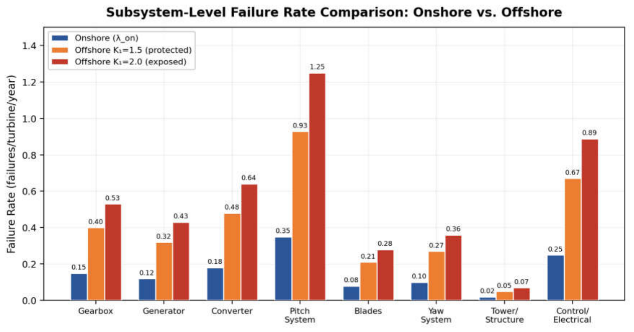
Figure 6.
Simulated wind farm availability by maintenance strategy (offshore, K₁ = 1.5, 25-year project). The AI-enhanced predictive strategy achieves 93.8% availability with 543 h/yr of downtime per turbine.
Figure 6.
Simulated wind farm availability by maintenance strategy (offshore, K₁ = 1.5, 25-year project). The AI-enhanced predictive strategy achieves 93.8% availability with 543 h/yr of downtime per turbine.
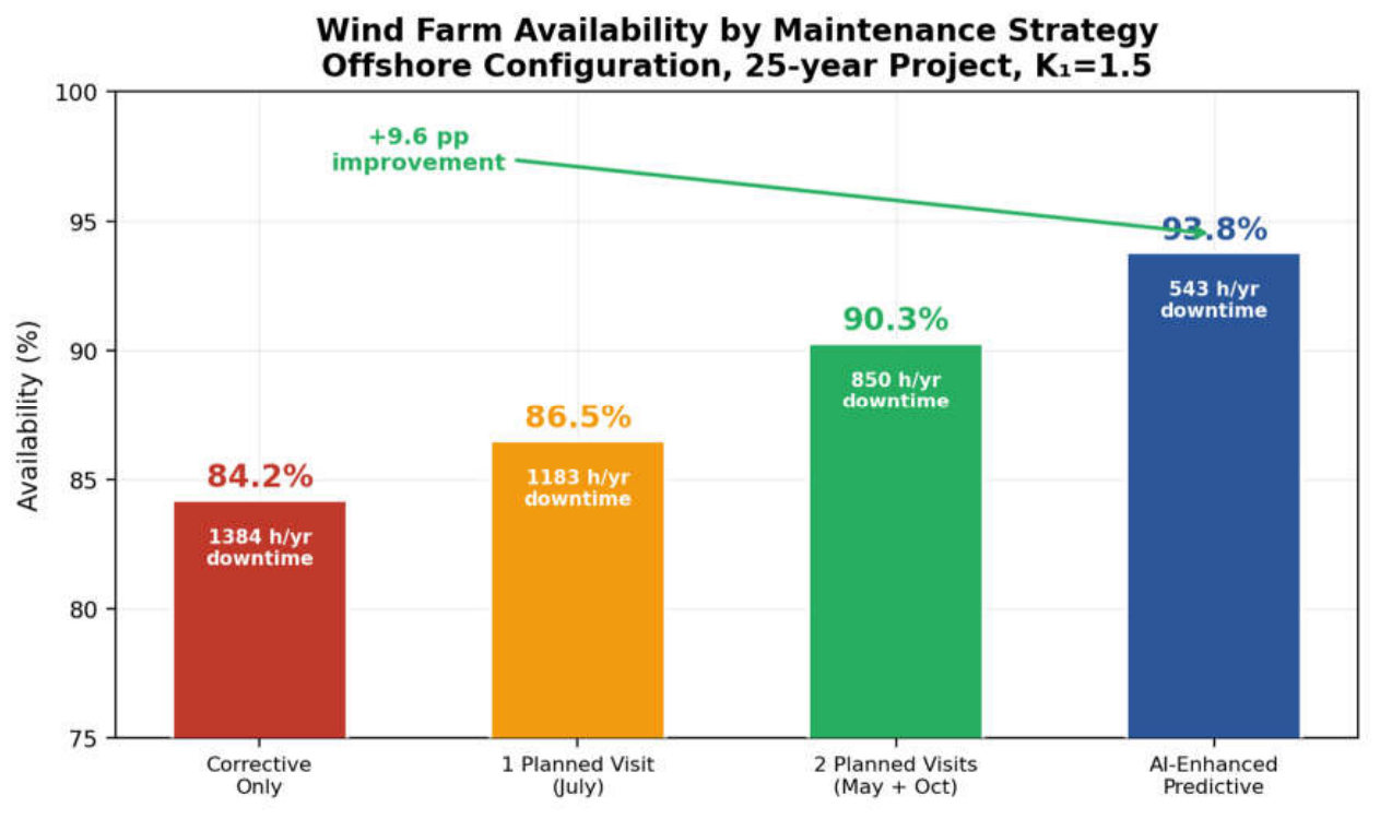
Figure 7.
Distribution of simulated (a) LCOE and (b) wind farm availability across the 10,000 Monte Carlo iterations for the four maintenance strategies (dashed lines: distribution means). Planned-intervention and AI-enhanced strategies both shift and narrow the distributions, reducing exposure to worst-case operational outcomes.
Figure 7.
Distribution of simulated (a) LCOE and (b) wind farm availability across the 10,000 Monte Carlo iterations for the four maintenance strategies (dashed lines: distribution means). Planned-intervention and AI-enhanced strategies both shift and narrow the distributions, reducing exposure to worst-case operational outcomes.
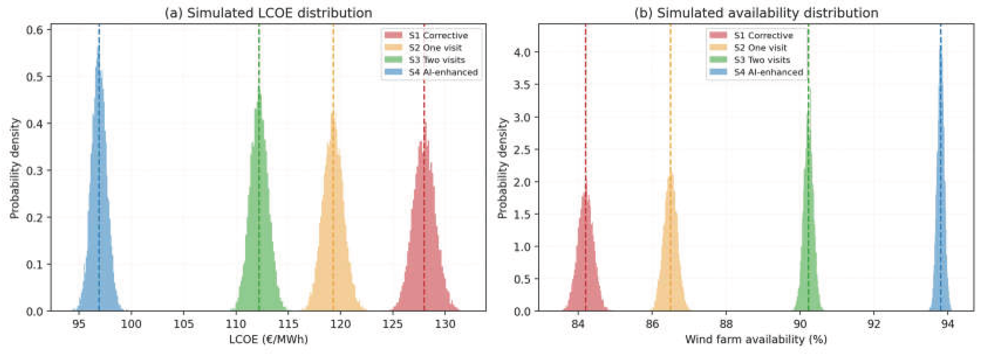
Figure 8.
Individual performance of the three AI modules evaluated in the simulation environment: (a) confusion matrix and ROC curve of the XGBoost fault-detection classifier at the selected operating threshold; (b) calibration of predicted failure probabilities against observed frequencies; (c) learning convergence of the deep Q-network scheduling agent (200-episode moving average of episodic reward).
Figure 8.
Individual performance of the three AI modules evaluated in the simulation environment: (a) confusion matrix and ROC curve of the XGBoost fault-detection classifier at the selected operating threshold; (b) calibration of predicted failure probabilities against observed frequencies; (c) learning convergence of the deep Q-network scheduling agent (200-episode moving average of episodic reward).
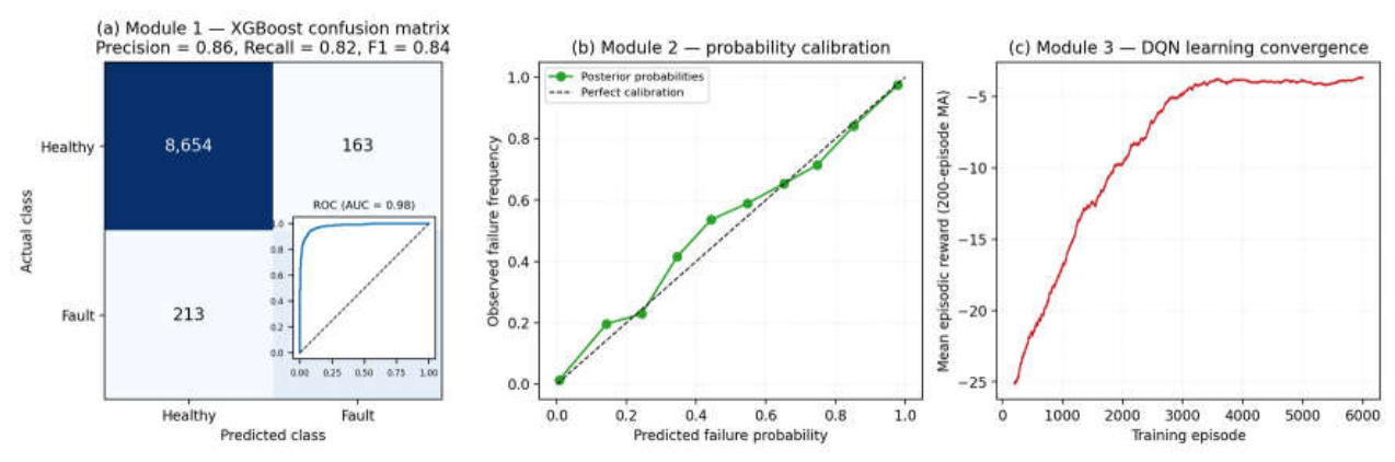
Figure 9.
LCOE sensitivity tornado diagram (base case = 65 €/MWh). WACC, capacity factor and failure rate are the three dominant drivers.
Figure 9.
LCOE sensitivity tornado diagram (base case = 65 €/MWh). WACC, capacity factor and failure rate are the three dominant drivers.
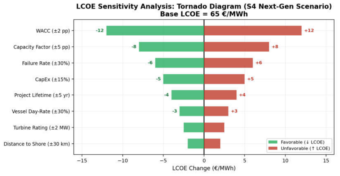

Table 1.
Subsystem-level failure rate translation with Weibull shape parameters, repair characteristics and cost estimates.
Table 1.
Subsystem-level failure rate translation with Weibull shape parameters, repair characteristics and cost estimates.
| Subsystem | λ_on (f/yr) | β (–) | λ_off K₁=1.5 | λ_off K₁=2.0 | MTTR (h) | Cost/failure | Annual cost (€/turbine) | Downtime (h/yr) |
| Gearbox | 0.15 | 1.8 | 0.40 | 0.53 | 168 | €95K | €38,000 | 67 |
| Generator | 0.12 | 1.6 | 0.32 | 0.43 | 120 | €65K | €20,800 | 38 |
| Converter | 0.18 | 1.3 | 0.48 | 0.64 | 36 | €18K | €8,640 | 17 |
| Pitch system | 0.35 | 1.2 | 0.93 | 1.25 | 24 | €8K | €10,000 | 30 |
| Blades | 0.08 | 2.1 | 0.21 | 0.28 | 96 | €120K | €33,600 | 27 |
| Yaw system | 0.10 | 1.4 | 0.27 | 0.36 | 18 | €5K | €1,800 | 6 |
| Tower/Structure | 0.02 | 2.5 | 0.05 | 0.07 | 240 | €200K | €14,000 | 17 |
| Control/Electrical | 0.25 | 1.1 | 0.67 | 0.89 | 12 | €3K | €2,010 | 11 |
| Total | 1.25 | — | 3.33 | 4.45 | — | — | €128,850 | 213 |
Table 2.
Performance comparison across maintenance strategies: mean ± standard deviation over 10,000 Monte Carlo iterations, with the 95% interval of simulated outcomes in brackets. Vessel utilization and CO₂ rows are deterministic accounting outputs of the logistics model.
Table 2.
Performance comparison across maintenance strategies: mean ± standard deviation over 10,000 Monte Carlo iterations, with the 95% interval of simulated outcomes in brackets. Vessel utilization and CO₂ rows are deterministic accounting outputs of the logistics model.
| Metric | S1 Corrective | S2 One visit | S3 Two visits | S4 AI-enhanced | AI vs S1 | Δ% |
| Availability (%) | 84.2 ± 0.2 [83.8, 84.6] | 86.5 ± 0.2 [86.1, 86.8] | 90.2 ± 0.1 [90.0, 90.5] | 93.8 ± 0.1 [93.6, 94.0] | +9.6 pp | — |
| Annual energy (GWh) | 450 ± 3 [444, 456] | 462 ± 3 [456, 469] | 482 ± 3 [476, 489] | 501 ± 4 [494, 508] | +51 | +11.4% |
| LCOE (€/MWh) | 128.0 ± 1.1 [125.9, 130.1] | 119.3 ± 1.0 [117.4, 121.2] | 112.2 ± 0.9 [110.5, 113.9] | 96.9 ± 0.7 [95.5, 98.3] | −31.1 | −24.3% |
| O&M (k€/MW/yr) | 142 ± 1 [140, 144] | 125 ± 1 [123, 127] | 118 ± 1 [116, 120] | 80 ± 1 [79, 81] | −62 | −43.7% |
| Downtime (h/yr) | 1,384 ± 18 [1348, 1420] | 1,183 ± 16 [1152, 1214] | 856 ± 11 [834, 878] | 543 ± 8 [527, 559] | −841 | −60.8% |
| Vessel utilization (%) | 45 | 55 | 62 | 81 | +36 pp | — |
| CO₂ (t/yr) | 485 | 342 | 315 | 248 | −237 | −48.9% |
| CO₂ (g/MWh) | 1,081 | 740 | 653 | 496 | −585 | −54.1% |
Disclaimer/Publisher’s Note: The statements, opinions and data contained in all publications are solely those of the individual author(s) and contributor(s) and not of MDPI and/or the editor(s). MDPI and/or the editor(s) disclaim responsibility for any injury to people or property resulting from any ideas, methods, instructions or products referred to in the content. |
© 2026 by the authors. Licensee MDPI, Basel, Switzerland. This article is an open access article distributed under the terms and conditions of the Creative Commons Attribution (CC BY) license (http://creativecommons.org/licenses/by/4.0/).
Copyright: This open access article is published under a Creative Commons CC BY 4.0 license, which permit the free download, distribution, and reuse, provided that the author and preprint are cited in any reuse.