Geometry and Dynamics of Observation Space in PODA: Binary Correlation Bounds and the Mass Spectrum of Joint Excitations

1. Observation Dimension and Correlation Bounds

The CHSH expression involves two binary observables at each of two sites. Enlarging the local Hilbert space may change the support of the state, the ranks of the event projections, and the family of realizable measurements. These changes impose different constraints on the correlation optimum. The universal quantum bound allows the preparation and local observables to be optimized together; the attainable bound for a fixed state depends on the measurement freedom that remains. A passage from ${\mathbb{CP}}^1$ to higher-dimensional observation spaces must therefore specify what is held fixed in the preparation and what is allowed to vary in the measurements.

PODA describes observation through admissible pairings of physical and observation states. Its set-theoretic foundations identify the two state roles and their joint domain[1], while phase transport supplies a covariant comparison between observation states[2]. Under the stated conditions on coherent responses, phase structure, and independent composition, the quantum representation gives projective events and the Born trace pairing[3,4]. We adopt this representation throughout the correlation analysis. Its positivity, local spectral constraints, and composition rule are the premises of the bounds derived below.

The real Gram representation reduces binary correlations to vector pairings in a common inner-product space. It recovers the Tsirelson bound and shows that a saturating configuration needs only two dimensions. This established result provides the reference point for the higher-dimensional problem. We then obtain the exact attainable bounds for arbitrary-rank binary projections and rank-one events on a fixed maximally entangled state, identifying the separate roles of uniform Schmidt support and projection rank. Comparing the two families at the same preparation distinguishes an extension of the measurement family from a change in the state resource. For restricted direction families, the optimization retains the actual admissible domains; the singular-value formula for complete Euclidean direction families applies only under its stated geometric assumptions.

Event geometry determines the structure of probability pairing, whereas an energy spectrum requires a dynamics. Section 7 introduces a joint field with positive gradient energy along observation space and relates the covariant eigenvalues of a fixed background to four-dimensional mass squared. Section 8 evaluates this spectrum on the full ${\mathbb{CP}}^1$ of the two-channel projective representation, with the phase weight specified through the Hopf connection. The resulting reconstruction of two mass scales and the tests involving higher levels are developed in Section 9. The local mass coefficient remains independent: geometry fixes the coefficients at each level without selecting the ratio of the two scales. Section 10 discusses the physical interpretation of the joint modes and their coupling to gravity.

2. Dual-Axis Pairing and Higher-Dimensional Observation Events

2.1. Quantum Representation of Binary Correlations

Let $\mathcal{X}$ and $\mathcal{S}$ denote the physical-state and observation-state spaces. Following the foundational dual-axis formulation, the admissible domain and the law of observed facts are written as

$$\mathcal{B}\hookrightarrow \mathcal{X}\times \mathcal{S},F:\mathcal{B}⟶\mathcal{Y}.$$

(1)

In a probabilistic representation, F assigns a distribution of observation outcomes. In a Bell experiment, the preparation is specified on the physical axis, while the two local settings jointly specify the observation state.

We adopt the Born representation and independent-composition conditions of Refs. [3,4], extended to a finite number d of channels. For a preparation x, let ${\rho }_x$ be the corresponding density operator. The local binary events satisfy

$$M_{\alpha |i}⪰0,\sum _{\alpha =\pm 1}{M}_{\alpha |i}={\mathbb{I}}_A,N_{\beta |j}⪰0,\sum _{\beta =\pm 1}{N}_{\beta |j}={\mathbb{I}}_B.$$

(2)

The joint probabilities are given by the dual-axis pairing

$$p(\alpha ,\beta |x,i,j)=Tr\left[{\rho }_x(M_{\alpha |i}\otimes N_{\beta |j})\right].$$

(3)

The associated self-adjoint contractions are $A_i=M_{+|i}-M_{-|i}$ and $B_j=N_{+|j}-N_{-|j}$, so that

$$E_{ij}=Tr\left[{\rho }_x(A_i\otimes B_j)\right],S_{\mathrm{CHSH}}=E_{00}+E_{01}+E_{10}-E_{11}.$$

(4)

All four correlations refer to the same preparation ensemble. For projective measurements, $A_i^2=B_j^2=\mathbb{I}$. Completeness of the local events makes each marginal distribution independent of the remote setting. The correlation bound also depends on Born positivity, the local spectral constraints, and the composition structure. These conditions on the quantum representation are assumed throughout the following derivation.

2.2. Event Manifolds, Projection Rank, and Gram Rank

In the coherent response space ${\mathbb{C}}^d$, normalized vectors modulo a common phase form the rank-one event space

$${\mathcal{F}}_d=S^{2d-1}/U\left(1\right)={\mathbb{CP}}^{d-1},{dim}_{\mathbb{R}}{\mathcal{F}}_d=2d-2.$$

(5)

For $d=2$, a rank-one event and its orthogonal complement are both one-dimensional; hence ${\mathbb{CP}}^1\simeq S^2$ parameterizes all nontrivial binary projective measurements with labelled outcomes, where both outcomes are present. For $d>2$, the rank of the positive-outcome projection must also be specified. A general binary projective observable has the form

$$A=2P-\mathbb{I},P^2=P=P^{†},rankP=k.$$

(6)

The event space at fixed rank k is the complex Grassmann manifold

$$Gr(k,d)=U\left(d\right)/(U\left(k\right)\times U(d-k)),{dim}_{\mathbb{R}}Gr(k,d)=2k(d-k).$$

(7)

Its real dimension is the dimension $d^2$ of $U\left(d\right)$ minus the stabilizer dimension $k^2+{(d-k)}^2$. The case $k=1$ gives ${\mathbb{CP}}^{d-1}$. Binary projections of arbitrary rank range over the different $Gr(k,d)$, whereas rank-one events remain confined to a single projective manifold.

These manifold dimensions are distinct from the real Gram rank $r_G$ of the correlation vectors, defined as the dimension of the span of the four vectors. There is no general equality between $r_G$ and either d or $2d-2$. The next section shows that a CHSH-saturating configuration has precisely $r_G=2$.

2.3. Positivity and Spectral Constraints in Higher-Dimensional Bloch Representations

For a qubit, the Pauli operators satisfy ${(a·\sigma )}^2={∥a∥}^2\mathbb{I}$, so every Euclidean unit direction defines a sharp binary observable. A general traceless Hermitian basis in higher dimension has no such property. For a three-level system, consider

$${\lambda }_8={\displaystyle \frac{1}{\sqrt{3}}}diag(1,1,-2),\rho ={\displaystyle \frac{{\mathbb{I}}_3}{3}}+{\displaystyle \frac{1}{2}}{r}_8{\lambda }_8.$$

(8)

At $r_8=2/\sqrt{3}$, the Bloch vector reaches the pure-state radius in this normalization, yet the resulting matrix is

$$\rho =diag(2/3,2/3,-1/3).$$

(9)

Its negative eigenvalue excludes it as a physical state. Moreover, the unit coordinate direction ${\lambda }_8$ has operator norm $2/\sqrt{3}>1$, outside the spectral range of a binary observable. Higher-dimensional correlations must therefore be optimized over an admissible domain that respects both state positivity and the spectral constraints on observations.

3. The Tsirelson Bound and the Geometry of Saturation

3.1. A Real Gram Representation of the Born Pairing

Lemma 3.1

(Correlation-vector representation). The correlations defined by Eqs. (3)–(4) admit a representation $E_{ij}=u_i·v_j$, where $u_0,u_1,v_0,v_1$ lie in a common real Hilbert space and each has norm at most 1.

Proof. 

Set ${\widehat{A}}_i=A_i\otimes {\mathbb{I}}_B$ and ${\widehat{B}}_j={\mathbb{I}}_A\otimes B_j$. In the realification of Hilbert–Schmidt space, take

$$u_i={\widehat{A}}_i{\rho }_x^{1/2},v_j={\widehat{B}}_j{\rho }_x^{1/2},U·V=ReTr\left(U^{†}V\right).$$

(10)

Since operators at opposite sites commute, $u_i·v_j=Tr\left({\rho }_x{\widehat{A}}_i{\widehat{B}}_j\right)=E_{ij}$. The contraction conditions give

$${∥u_i∥}^2=Tr\left({\rho }_x{\widehat{A}}_i^2\right)\le 1,{∥v_j∥}^2\le 1.$$

(11)

The square root of a trace-class density operator is Hilbert–Schmidt. The construction therefore extends to infinite-dimensional spaces without recourse to a finite-dimensional Bloch representation.    □

Theorem 3.2

(Dimension-independent bound and saturation conditions). Under the quantum-representation conditions stated above, the correlations satisfy

$$|S_{\mathrm{CHSH}}|\le 2\sqrt{2}$$

(12)

in every dimension. Positive saturation, $S_{\mathrm{CHSH}}=2\sqrt{2}$, holds if and only if

$$∥v_0∥=∥v_1∥=1,v_0·v_1=0,u_0={\displaystyle \frac{v_0+v_1}{\sqrt{2}}},u_1={\displaystyle \frac{v_0-v_1}{\sqrt{2}}}.$$

(13)

The four vectors of a saturating correlation thus span a common real two-dimensional plane.

Proof. 

In the real Gram representation,

$$\begin{array}{cc}\hfill |S_{\mathrm{CHSH}}|& \le ∥v_0+v_1∥+∥v_0-v_1∥\hfill \\ \hfill & \le \sqrt{2\left({∥v_0+v_1∥}^2+{∥v_0-v_1∥}^2\right)}\hfill \\ \hfill & =2\sqrt{{∥v_0∥}^2+{∥v_1∥}^2}\le 2\sqrt{2}.\hfill \end{array}$$

(14)

The second step is the Cauchy inequality and the third is the parallelogram identity. Neither depends on dimension.

Equality in the last step requires $∥v_0∥=∥v_1∥=1$. Equality in the second requires the sum and difference vectors to have the same norm, or equivalently $v_0·v_1=0$. Both norms then equal $\sqrt{2}$. For positive saturation, equality in the first step further requires $u_0$ and $u_1$ to be the unit vectors along the sum and difference, respectively, yielding Eq. (13). Substitution proves sufficiency.    □

Figure 1. A CHSH-saturating configuration. All four vectors arise from the Hilbert–Schmidt representation of a single state. The vectors $v_0$ and $v_1$ are orthogonal, while $u_0$ and $u_1$ lie along their sum and difference. Saturation confines all correlation vectors to a common real two-dimensional subspace.

Figure 1. A CHSH-saturating configuration. All four vectors arise from the Hilbert–Schmidt representation of a single state. The vectors $v_0$ and $v_1$ are orthogonal, while $u_0$ and $u_1$ lie along their sum and difference. Saturation confines all correlation vectors to a common real two-dimensional subspace.

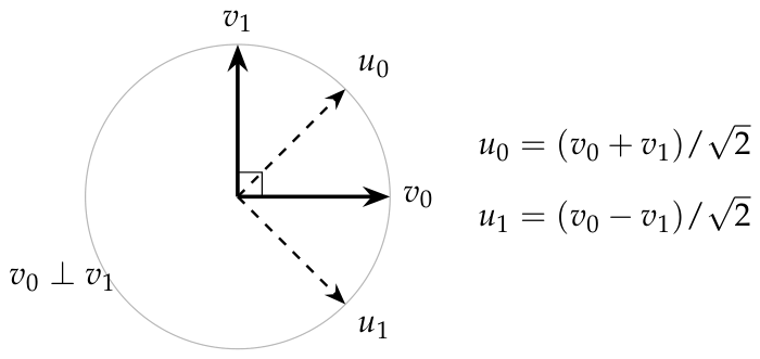
For unit vectors $v_0,v_1$, write $c=v_0·v_1$. The bound becomes

$$|S_{\mathrm{CHSH}}|\le \sqrt{2+2c}+\sqrt{2-2c}\le 2\sqrt{2}.$$

(15)

If all correlation vectors lie on a single real line, then

$$|S_{\mathrm{CHSH}}|\le |v_0+v_1|+|v_0-v_1|=2max(|v_0|,|v_1\left|\right)\le 2.$$

(16)

A collinear configuration therefore attains at most 2. If the available direction space has dimension at least two and contains every unit direction, the geometric optimum is $2\sqrt{2}$, and every saturating configuration has $r_G=2$. Gram rank describes the linear support of the vectors; it is not, by itself, a criterion of classicality. For a specified observation family, saturation also requires that all four directions in Eq. (13) be simultaneously realizable.

3.2. Local Noncommutativity

For binary projective measurements, define the CHSH operator

$$\mathcal{C}=A_0\otimes (B_0+B_1)+A_1\otimes (B_0-B_1).$$

(17)

Using $A_i^2=B_j^2=\mathbb{I}$, expansion gives

$${\mathcal{C}}^2=4\mathbb{I}-[A_0,A_1]\otimes [B_0,B_1].$$

(18)

Each commutator has norm at most 2, whence ${∥\mathcal{C}∥}^2\le 8$, recovering the operator bound in Ref. [3]. Equation (18) ties the enhancement of binary projective correlations to local noncommutativity. The Gram proof expresses the same constraint through inner-product geometry. The operator identity requires self-adjoint reflections; the Gram argument already covers general binary POVMs.

3.3. Saturating Constructions in Higher-Dimensional Spaces

Choose a controllable two-dimensional subspace at each site, prepare

$$|{\Phi }_2\rangle ={\displaystyle \frac{|00\rangle +|11\rangle }{\sqrt{2}}},$$

(19)

and set

$$B_0=Z,B_1=X,A_0={\displaystyle \frac{Z+X}{\sqrt{2}}},A_1={\displaystyle \frac{Z-X}{\sqrt{2}}},$$

(20)

where $X,Z$ are Pauli matrices. These settings attain $2\sqrt{2}$. Each observable may be extended arbitrarily as a reflection on the corresponding orthogonal complement. The preparation has no support on either complement, so the saturation value includes all events and requires no postselection.

Thus, whenever $d_A,d_B\ge 2$ and both the state and observations may be chosen, the universal optimum is $2\sqrt{2}$. Fixing a state with full local Schmidt support removes the freedom to concentrate all weight on two Schmidt modes. This is the source of the dimension dependence derived next.

4. Exact Attainable Bounds for a Fixed Higher-Dimensional State

4.1. Uniform Schmidt Support and Trace-Norm Optimization

For a fixed state and specified local observation families, write $\beta =sup|S_{\mathrm{CHSH}}|$. If the families are closed under outcome relabelling, this also equals $sup{S}_{\mathrm{CHSH}}$. Throughout this section, the state is fixed to the maximally entangled state of two d-dimensional systems,

$$|{\Phi }_d\rangle ={\displaystyle \frac{1}{\sqrt{d}}}{\displaystyle \sum _{k=0}^{d-1}}|k\rangle \otimes |k\rangle .$$

(21)

Its d Schmidt coefficients are equal. For arbitrary local matrices,

$$\langle {\Phi }_d|A\otimes B|{\Phi }_d\rangle ={\displaystyle \frac{1}{d}}Tr\left(A^{\mathsf{T}}B\right),$$

(22)

where transposition is taken in the Schmidt basis of Eq. (21).

Lemma 4.1

(Trace-norm optimization at one site). For fixed self-adjoint reflections $B_0,B_1$ at Bob’s site, optimization over all self-adjoint reflections at Alice’s site gives

$$\underset{A_0,A_1}{max}{S}_{\mathrm{CHSH}}={\displaystyle \frac{{∥B_0+B_1∥}_1+{∥B_0-B_1∥}_1}{d}},$$

(23)

where ${∥C∥}_1=Tr\sqrt{C^{†}C}$ is the trace norm.

Proof. 

Let $c_k$ be the eigenvalues of a Hermitian matrix C. For every self-adjoint contraction D, the spectral decomposition gives $Tr\left(DC\right)\le {\sum }_k\left|c_k\right|$. Equality is attained by $D=sgnC$, with either sign chosen on the null space. Applying Eq. (22) and optimizing $A_0^{\mathsf{T}}$ and $A_1^{\mathsf{T}}$ separately proves the claim. The optimization includes all reflections at Alice’s site, including those that mix different subspaces.    □

4.2. Two-Dimensional Invariant Blocks of Two Reflections

Lemma 4.2

(Common invariant-subspace decomposition). Two self-adjoint reflections $B_0,B_1$ on a finite-dimensional space admit a common orthogonal decomposition into invariant subspaces of dimension at most 2.

Proof. 

Set $U=B_0{B}_1$. Then U is unitary and $B_{0}U{B}_0=U^{†}$. If $Uv=\lambda v$, then $U\left(B_{0}v\right)=\overline{\lambda }{B}_{0}v$. Choose one representative $\lambda$ from each nonreal conjugate pair and an orthonormal basis $v_{\alpha }$ of its eigenspace. Each pair $v_{\alpha },B_0{v}_{\alpha }$ spans a two-dimensional subspace invariant under both $B_0$ and $B_1=B_{0}U$; these subspaces are mutually orthogonal. Within the eigenspaces of $\lambda =\pm 1$, one has $B_1=\pm B_0$, and simultaneous diagonalization gives one-dimensional blocks. Together these subspaces exhaust the Hilbert space.    □

Theorem 4.3

(Even–odd attainable bounds for fixed ${\Phi }_d$). For the fixed state in Eq. (21), optimization over all binary projective measurements of arbitrary rank yields

$${\beta }_d^{\mathrm{all}}=\left\{\begin{array}{cc}2\sqrt{2},\hfill & d\mathit{even},\hfill \\ 2\sqrt{2}-{\displaystyle \frac{2\sqrt{2}-2}{d}},\hfill & d\mathit{odd}.\hfill \end{array}\right.$$

(24)

We take $d\ge 2$ below. If trivial binary measurements are admitted, the formula also gives 2 for $d=1$.

Proof. 

Suppose the decomposition in Lemma 4.2 contains m two-dimensional blocks and k one-dimensional blocks, so that $d=2m+k$. On a one-dimensional block, $B_0$ and $B_1$ are each $\pm 1$, and their contribution to the numerator of Eq. (23) is always 2.

On an irreducible two-dimensional block, write $B_j=n_j·\sigma$ with unit vectors $n_j$. If $n_0·n_1=c$, the block contributes

$$2\sqrt{2+2c}+2\sqrt{2-2c}\le 4\sqrt{2}.$$

(25)

Adding the trace norms of all blocks gives

$$S_{\mathrm{CHSH}}\le {\displaystyle \frac{4\sqrt{2}m+2k}{d}}=2\sqrt{2}-{\displaystyle \frac{(2\sqrt{2}-2)k}{d}}.$$

(26)

For even d, one may take $k=0$; for odd d, necessarily $k\ge 1$. This proves the stated upper bounds.

The settings in Eq. (20) contribute $4\sqrt{2}$ on each two-dimensional block. For odd d, choose $B_0=B_1=A_0=A_1=1$ on the remaining one-dimensional block, which contributes 2. The direct sums of these observables attain Eq. (24), so the bounds are exact.    □

For odd-dimensional uniform Schmidt support, a one-dimensional reflection block carries nonzero weight, but its CHSH contribution cannot exceed the classical bound. A state supported on two dimensions avoids this loss and still attains $2\sqrt{2}$. Accordingly, d in Eq. (24) refers specifically to the dimension of the uniform Schmidt support of ${\Phi }_d$.

Corollary 4.4

(Optimum over binary POVMs). For fixed ${\Phi }_d$, the optimum over all binary POVMs is again given by Eq. (24).

Proof. 

Finite-dimensional self-adjoint contractions form the compact convex set $\{A:-\mathbb{I}\le A\le \mathbb{I}\}$, whose extreme points are precisely the reflections. If A has an eigenvalue strictly inside $(-1,1)$, small perturbations of opposite sign along the corresponding spectral projection give a nontrivial convex decomposition. Conversely, if the spectrum consists only of $\pm 1$, every operator in a convex decomposition must take the same extremal values along the saturated spectral directions. Positivity forces the off-diagonal blocks to vanish, leaving only the trivial decomposition. CHSH is linear in each observable separately. Starting from any maximizing quadruple, one may therefore replace each observable in turn by an extreme point maximizing the corresponding linear functional, without changing the optimum. All four observables can thus be taken to be reflections.    □

4.3. The Attainable Bound for Rank-One Events

Restrict the positive outcome to a rank-one projection $P_a=|a\rangle \langle a|$, with complementary event $\mathbb{I}-P_a$. The binary observable is then

$$A\left(a\right)=2|a\rangle \langle a|-\mathbb{I},\left[a\right]\in {\mathbb{CP}}^{d-1}.$$

(27)

Together with outcome relabelling, this family contains all nontrivial binary projective measurements for $d=2,3$. Starting at $d=4$, intermediate-rank projections supply additional observation events.

Theorem 4.5

(Exact bound under the rank-one event restriction). For fixed ${\Phi }_d$, with all four local observables restricted to Eq. (27) and outcome relabellings thereof, one has, for $d\ge 2$,

$${\beta }_d^{\left(1\right)}=2+{\displaystyle \frac{4\sqrt{2}-4}{d}}.$$

(28)

Proof. 

The ranges of Bob’s two rank-one projections span a subspace W of dimension at most 2. On $W^{\perp }$, both reflections are $-\mathbb{I}$, contributing 2 per dimension to the numerator of Eq. (23). If $dimW=2$, this block contributes at most $4\sqrt{2}$. Temporarily allowing Alice all reflections therefore gives

$$|S_{\mathrm{CHSH}}|\le {\displaystyle \frac{4\sqrt{2}+2(d-2)}{d}}=2+{\displaystyle \frac{4\sqrt{2}-4}{d}}.$$

(29)

If $dimW=1$, the two reflections are simultaneously diagonalizable. Each one-dimensional block contributes 2, giving a CHSH bound of 2. Relabelling the outcomes of either of Bob’s observables only exchanges the two trace norms or reverses an overall sign inside a norm, so the bound is unchanged.

Choose the settings in Eq. (20) on $W=span\left\{\right|0\rangle ,|1\rangle \}$ and extend all four reflections by $-\mathbb{I}$ on $W^{\perp }$. Every reflection has a one-dimensional $+1$ eigenspace, satisfying the rank-one restriction at both sites. The two-dimensional block contributes $4\sqrt{2}$, while each of the remaining $d-2$ dimensions contributes 2. The bound is attained.    □

Whatever the dimension of the event manifold, the ranges of two local rank-one projections span at most two dimensions. Since ${\Phi }_d$ distributes its weight uniformly over all channels, the other $d-2$ directions contribute only a classical background in the optimal construction. The excess above the classical bound consequently decays as $1/d$.

5. Restricted Direction Families and Correlation Extrema

5.1. The Support Function of the Observation Domain

Suppose the correlations of a fixed physical state admit the bilinear representation $E(a,b)=a^{\mathsf{T}}Tb$, with admissible directions in ${\mathcal{D}}_A$ and ${\mathcal{D}}_B$. Define the support function of Alice’s observation domain by

$$h_A\left(z\right)=\underset{a\in {\mathcal{D}}_A}{sup}{a}^{\mathsf{T}}z.$$

(30)

Optimizing Alice’s two settings separately gives

$$\beta (T;{\mathcal{D}}_A,{\mathcal{D}}_B)=\underset{b_0,b_1\in {\mathcal{D}}_B}{sup}\left[h_A\left(T(b_0+b_1)\right)+h_A\left(T(b_0-b_1)\right)\right].$$

(31)

The direction domains are assumed to be closed under outcome relabelling, so the positive supremum equals the supremum of the absolute value. All observation constraints remain encoded in the support function and in Bob’s admissible domain. In the PODA representation, the attainable bound for a fixed physical state thus depends directly on the available observation events.

5.2. A Singular-Value Formula for Complete Direction Families

Theorem 5.1

(Optimum for a bilinear direction family). Suppose ${\mathcal{D}}_A=S^{m-1}$ and ${\mathcal{D}}_B=S^{n-1}$, each local setting may independently range over all Euclidean unit directions, and the same real matrix T defines all four correlations. Then

$$\beta \left(T\right)=2\sqrt{s_1{\left(T\right)}^2+s_2{\left(T\right)}^2},$$

(32)

where $s_1\ge s_2\ge 0$ are the two largest singular values of T, with zero padding if fewer than two are present.

Proof. 

For $n\ge 2$, any two unit directions at Bob’s site may be written as

$$b_0+b_1=2cos\theta c,b_0-b_1=2sin\theta e,c\perp e,∥c∥=∥e∥=1,$$

(33)

with $0\le \theta \le \pi /2$. If either the sum or the difference vanishes, its direction may be chosen as any unit vector orthogonal to the other. Optimizing Alice’s settings along $Tc$ and $Te$, and then optimizing over $\theta$, gives

$$\beta \left(T\right)=2\underset{c\perp e}{max}\sqrt{{∥Tc∥}^2+{∥Te∥}^2}.$$

(34)

Let $K=T^{\mathsf{T}}T$ have eigenvalues ${\lambda }_1\ge {\lambda }_2\ge \dots$. In its eigenbasis, the quantity under the square root is ${\sum }_{\ell }{\lambda }_{\ell }{w}_{\ell }$, where $w_{\ell }=|c_{\ell }{|}^2+{\left|e_{\ell }\right|}^2\in [0,1]$ and ${\sum }_{\ell }{w}_{\ell }=2$. Its maximum is ${\lambda }_1+{\lambda }_2$, attained when $c,e$ are the first two eigenvectors. Since ${\lambda }_j=s_j^2$, this proves Eq. (32). For $n=1$, the optimum is directly $2s_1$.    □

For $n\ge 2$, choose $c,e$ as the first two right singular vectors. Corresponding optimal settings are

$$\begin{array}{cc}\hfill a_0& =Tc/s_1,a_1=Te/s_2,\hfill \\ \hfill b_0& ={\displaystyle \frac{s_{1}c+s_{2}e}{\sqrt{s_1^2+s_2^2}}},b_1={\displaystyle \frac{s_{1}c-s_{2}e}{\sqrt{s_1^2+s_2^2}}}.\hfill \end{array}$$

(35)

Alice’s direction associated with a zero singular value is arbitrary; if $T=0$, every setting gives zero correlation. When every unit direction defines a valid binary observable, $\left|E\right(a,b\left)\right|\le 1$ implies $s_1\le 1$, and Eq. (32) remains bounded by $2\sqrt{2}$. This extends the spectral optimization of the PODA qubit correlation tensor [3,4] to complete Euclidean direction families. A general higher-dimensional event domain is not a complete sphere, and its optimum must still be determined from the actual domains ${\mathcal{D}}_A,{\mathcal{D}}_B$.

Anticommuting Hermitian matrices provide higher-dimensional realizations of complete direction families. If

$${\Gamma }_{\ell }{\Gamma }_j+{\Gamma }_j{\Gamma }_{\ell }=2{\delta }_{\ell j}\mathbb{I},A\left(a\right)=\sum _{\ell }{a}_{\ell }{\Gamma }_{\ell },$$

(36)

then $A{\left(a\right)}^2=\mathbb{I}$ for every unit vector a. In dimension $D=2^k$, one may take the Pauli tensor products

$$\begin{array}{cc}\hfill {\Gamma }_{2j-1}& =Z^{\otimes (j-1)}\otimes X\otimes {\mathbb{I}}^{\otimes (k-j)},\hfill \\ \hfill {\Gamma }_{2j}& =Z^{\otimes (j-1)}\otimes Y\otimes {\mathbb{I}}^{\otimes (k-j)},1\le j\le k.\hfill \end{array}$$

(37)

On the state ${\Phi }_D$, choosing ${\Gamma }_{\ell }^{\mathsf{T}}$ for Bob gives $E(a,b)=a·b$. This observation family has $2k$ direction coordinates, although CHSH saturation requires only two orthogonal directions. Increasing their number enlarges the event family while leaving the norm constraints on the sum and difference unchanged.

6. Dimension Dependence and Experimental Comparison

6.1. Three Preparation and Observation Conditions

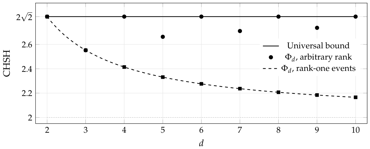
Table 1 gives the exact optima under three sets of constraints: the state may be supported on two dimensions; the state is fixed to ${\Phi }_d$ and projection ranks are unrestricted; or the state is fixed to ${\Phi }_d$ and events are restricted to rank one. At $d=4$, the respective values are $2\sqrt{2}$, $2\sqrt{2}$, and $1+\sqrt{2}$. The rank-one restriction lowers the attainable value for the specified state; the universal bound is unchanged.

Figure 2. Attainable CHSH values versus the dimension d of uniform Schmidt support. Arbitrary-rank observations exhibit an even–odd dependence, whereas the excess above the classical bound for rank-one events decays as $1/d$. The dimension d is integer-valued; the dashed curve is the continuous extension of the rank-one formula.

Figure 2. Attainable CHSH values versus the dimension d of uniform Schmidt support. Arbitrary-rank observations exhibit an even–odd dependence, whereas the excess above the classical bound for rank-one events decays as $1/d$. The dimension d is integer-valued; the dashed curve is the continuous extension of the rank-one formula.

6.2. Numerical Reproduction of the Explicit Constructions

The accompanying program verify_tsirelson.py constructs the local observable matrices for $d=2,\dots ,10$ and evaluates their correlations using Eq. (22). The arbitrary-rank construction uses direct sums of two-dimensional Pauli blocks, with one additional one-dimensional block in odd dimension. In the rank-one construction, Bob’s positive-outcome vectors are $|0\rangle$ and $(|0\rangle +|1\rangle )/\sqrt{2}$. Alice’s are the positive-eigenvalue eigenvectors of $B_0+B_1$ and $B_0-B_1$ within the same two-dimensional subspace.

The program checks Hermiticity, the identities $A_i^2=B_j^2=\mathbb{I}$, and the ranks of the positive-outcome projections. It compares the constructed values with Eqs. (24) and (28), with additional checks using valid randomly generated observables and a fixed seed. The analytic proofs establish the global optima; the numerical calculations reproduce their saturating constructions. The results are recorded in results.json.

6.3. Experimental Realization and Preparation Error

An experimental comparison must preserve the uniform Schmidt support in Eq. (21) and control the projection ranks of the two observation families. Using d distinguishable modes as a basis, a local mode transformation followed by a partition of the output ports into two groups realizes a binary projection. Assigning $+1$ to a single port gives a rank-one event; assigning several ports to the positive outcome permits higher-rank projections. Mode losses and local transformation errors require independent calibration.

Under identical preparation conditions, one compares the rank-one scheme with the arbitrary-rank scheme built from paired two-dimensional blocks. At $d=4$, their ideal values are $1+\sqrt{2}$ and $2\sqrt{2}$, separated by $\sqrt{2}-1\simeq 0.414214$. The difference directly reflects the change in available projection ranks. At $d=3$, both values equal $(4\sqrt{2}+2)/3$, so the optima do not distinguish the two observation constraints. These results are compatible with the standard quantum representation. The comparison tests event-rank restrictions for a fixed state and cannot, by itself, distinguish PODA from standard quantum mechanics.

All channels must enter the raw $\pm 1$ statistics. Assignments for no-click and multiple-click events, or the detection model governing those events, must also be specified in advance. Discarding modes and normalizing only to coincidence counts changes the support of the effective state, so Eq. (21) no longer describes the ensemble being counted. The four settings must also sample the same preparation ensemble to define the correlations in Eq. (4).

Preparation error can be bounded directly by trace distance. Let ${\rho }_{★}$ be the target state, $\rho$ the actual state, and $\epsilon =\frac{1}{2}{∥\rho -{\rho }_{★}∥}_1$. For any fixed valid CHSH operator,

$$\left|Tr\left[(\rho -{\rho }_{★})\mathcal{C}\right]\right|\le {∥\rho -{\rho }_{★}∥}_1∥\mathcal{C}∥\le 4\sqrt{2}\epsilon .$$

(38)

Taking the supremum over the same observation family bounds the difference between the optima by the same quantity, $4\sqrt{2}\epsilon$. This dimension-independent estimate controls the deviation from the ideal optimum due to preparation error.

7. A Joint Field on a Fixed Observation Background

7.1. Dynamical Assumptions

A correlation function specifies the probabilistic pairing of a prepared state with observation events. Energy requires, in addition, dynamical degrees of freedom and an action governing their evolution. The admissible joint domain of PODA provides a common setting for transport along the physical and observation directions and for their mixed transport[4]. We restrict attention to a regular, separable region of this domain and ask how covariant gradients along the observation directions enter the four-dimensional propagation spectrum.

Let spacetime be ${\mathcal{M}}^{1,3}$, with coordinates $y^{\mu }$, $y^0=ct$, and metric $\eta =diag(1,-1,-1,-1)$. The spacetime coordinate y and the physical-state label $x\in \mathcal{X}$ are distinct objects. In the region under consideration, the domain has the product form ${\mathcal{M}}^{1,3}\times \mathcal{S}$. The observation manifold $\mathcal{S}$ carries a positive-definite metric h, and a Hermitian line bundle $\mathcal{L}\to \mathcal{S}$ carries a compatible connection $D_S$; neither depends on y. The joint field $\Psi$ is a section of the pullback of this line bundle to the product space, with $\Psi (y,s)$ denoting its complex component in a local gauge frame. A trivial line bundle recovers the usual complex scalar field.

We assign independent dynamics to $\Psi$ and require its covariant gradients in the observation directions to contribute positive energy. This requirement supplements the dual-axis structure with a dynamical assumption. Excitations of $\Psi$ are determined by the field equation and initial conditions; relabelling a measurement setting does not excite the field. Local frames are pulled back from the observation line bundle, so their transition functions depend only on s. In these frames, the pullback connection satisfies ${\nabla }_{\mu }={\partial }_{\mu }$ and ${\nabla }_a=D_a$; its curvature in the spacetime directions and its mixed curvature both vanish. The action below is written in such a frame. A change to a y-dependent frame must transform the full connection, with spacetime derivatives then written as ${\nabla }_{\mu }$.

7.2. Action and Conserved Energy

Take the observation coordinates $s^a$ to be dimensionless, let $L_S>0$ have dimensions of length, and let $m_X\ge 0$ be the local mass parameter common to all modes. Consider the second-order action

$$\begin{array}{cc}\hfill \mathcal{I}[\Psi ]& =C_{\Psi }\int \mathrm{d}t{\mathrm{d}}^3\mathbf{y}\mathrm{d}{\mu }_h\left(s\right)\left[{\hslash }^2{\partial }_{\mu }{\Psi }^{*}{\partial }^{\mu }\Psi -m_X^2{c}^2{|\Psi |}^2-{\displaystyle \frac{{\hslash }^2}{L_S^2}}{|D_S\Psi |}_h^2\right],\hfill \end{array}$$

(39)

$$\begin{array}{cc}\hfill |D_S{\Psi |}_h^2& =h^{ab}{(D_a\Psi )}^{*}{D}_b\Psi .\hfill \end{array}$$

(40)

The positive constant $C_{\Psi }$ sets the field normalization and gives $\mathcal{I}$ the dimensions of action. All terms in brackets have the same dimensions. Their local expressions agree on overlaps of gauge charts and therefore define a global action. Equation (39) preserves spacetime Lorentz symmetry and gauge covariance of the observation connection. The coefficients of the mass term and the observation-gradient term are independent model parameters.

On the Hilbert space of sections $L^2(\mathcal{S},\mathcal{L};\mathrm{d}{\mu }_h)$, the observation operator is

$${\mathcal{K}}_S=D_S^{†}{D}_S,\langle \chi ,{\mathcal{K}}_S\chi \rangle ={\int }_{\mathcal{S}}{\left|D_S\chi \right|}_h^2\mathrm{d}{\mu }_h\ge 0.$$

(41)

We take $\mathcal{S}$ to be compact and without boundary. If a boundary is present, boundary conditions must be specified that define a nonnegative self-adjoint realization and preserve the identity above. Varying ${\Psi }^{*}$ and integrating by parts gives

$$\left[{\hslash }^2{\square }_y+m_X^2{c}^2+{\displaystyle \frac{{\hslash }^2}{L_S^2}}{\mathcal{K}}_S\right]\Psi =0,{\square }_y={\displaystyle \frac{1}{c^2}}{\partial }_t^2-{\nabla }_{\mathbf{y}}^2.$$

(42)

Time-translation symmetry of the background yields the conserved energy

$$H=C_{\Psi }\int {\mathrm{d}}^3\mathbf{y}\mathrm{d}{\mu }_h\left[{\displaystyle \frac{{\hslash }^2}{c^2}}|{\partial }_t{\Psi |}^2+{\hslash }^2|{\nabla }_{\mathbf{y}}{\Psi |}^2+m_X^2{c}^2{|\Psi |}^2+{\displaystyle \frac{{\hslash }^2}{L_S^2}}{|D_S\Psi |}_h^2\right]\ge 0.$$

(43)

The observation-gradient term has the same sign as the spatial-gradient term in the action and contributes a nonnegative quadratic form to the Hamiltonian. Its contribution to the squared mass is therefore nonnegative.

7.3. Spectral Decomposition and Four-Dimensional Rest Mass

Proposition 7.1

(Mass spectrum of the joint field). Let ${\lambda }_n\ge 0$ be the distinct eigenvalues of ${\mathcal{K}}_S$, with degeneracies $d_n$ and orthonormal eigensections satisfying

$${\mathcal{K}}_S{\chi }_{n\alpha }={\lambda }_n{\chi }_{n\alpha },\alpha =1,\dots ,d_n.$$

(44)

The four-dimensional excitations at spectral level n obey the dispersion relation

$$E_n^2=p^2{c}^2+m_X^2{c}^4+{\displaystyle \frac{{\hslash }^2{c}^2}{L_S^2}}{\lambda }_n=p^2{c}^2+M_n^2{c}^4,$$

(45)

where $p=\left|\mathbf{p}\right|$. Their mass and rest energy are

$$M_n^2=m_X^2+{\displaystyle \frac{{\hslash }^2}{c^2{L}_S^2}}{\lambda }_n,E_{0,n}=M_n{c}^2(M_n>0).$$

(46)

If $M_n=0$, the dispersion relation is $E_n=c\left|\mathbf{p}\right|$; this massless propagating mode has no rest frame.

Proof. 

Substituting the separated solution

$$\Psi (y,s)=exp\left(-{\displaystyle \frac{i{E}_{n}t}{\hslash }}+{\displaystyle \frac{i\mathbf{p}·\mathbf{y}}{\hslash }}\right){\chi }_{n\alpha }\left(s\right)$$

(47)

into Eq. (42) gives

$$-{\displaystyle \frac{E_n^2}{c^2}}+p^2+m_X^2{c}^2+{\displaystyle \frac{{\hslash }^2}{L_S^2}}{\lambda }_n=0.$$

(48)

Multiplication by $c^2$ gives the dispersion relation. For $M_n>0$, its positive-energy branch at $p=0$ gives the rest energy. For $M_n=0$, it reduces directly to the massless relation.

The spectral expansion $\Psi ={\sum }_n{\sum }_{\alpha =1}^{d_n}{\varphi }_{n\alpha }\left(y\right){\chi }_{n\alpha }\left(s\right)$ gives the same result. Substitution into the action and use of orthonormality yield

$$\mathcal{I}=C_{\Psi }\sum _n{\displaystyle \sum _{\alpha =1}^{d_n}}\int \mathrm{d}t{\mathrm{d}}^3\mathbf{y}\left[{\hslash }^2{\partial }_{\mu }{\varphi }_{n\alpha }^{*}{\partial }^{\mu }{\varphi }_{n\alpha }-M_n^2{c}^2{\left|{\varphi }_{n\alpha }\right|}^2\right].$$

(49)

Each observation eigensection defines a four-dimensional scalar mode of mass $M_n$, and the $d_n$ modes at a given level have equal mass. After field quantization, a single excitation obeys Eq. (45). The total energy of a classical field depends on its amplitude and is given by Eq. (43). □

For a massive mode, the observation gradient changes the composition of its mass, while its rest energy remains $E_{0,n}=M_n{c}^2$.

For $m_X>0$ and low observation excitations, ${\hslash }^2{\lambda }_n\ll m_X^2{c}^2{L}_S^2$, the rest energy expands as

$$E_{0,n}=m_X{c}^2+{\displaystyle \frac{{\hslash }^2{\lambda }_n}{2m_X{L}_S^2}}+O\left({\displaystyle \frac{{\hslash }^4{\lambda }_n^2}{m_X^3{c}^2{L}_S^4}}\right).$$

(50)

Here $m_X$ is a parameter in the action, whereas $M_n$ is the rest mass of the full mode. A measured value of $M_n$ already includes the observation-gradient contribution.

Compactness makes the observation spectrum discrete in this model. On a noncompact observation space with a continuous spectral component, the mode expansion must include the corresponding spectral integral. If h or $D_S$ depends on y, the eigensections also vary with y and generate derivative couplings between modes in the four-dimensional equations. The constant-mass decomposition in Eq. (45) then generally ceases to hold.

8. Intrinsic Geometry of the Two-Channel Observation Fiber

8.1. Projective Metric and Hopf Connection

The geometric content of the mass spectrum resides in ${\mathcal{K}}_S$. To specify this operator, we take the full fiber of pure observation states associated with a two-channel coherent response in PODA. Normalization followed by the quotient by the common phase gives the Hopf structure $S^3\to {\mathbb{CP}}^1$[3,4]. Its connection compares phases between observation states and agrees with the covariant form of local phase transport[2]. All calculations below take place on the regular projective space defined by nonzero responses.

In a local gauge chart, choose a representative with $z^{†}z=1$ and identify $z\sim e^{i\alpha }z$. The overlap of neighboring events defines the metric

$${1-|z\left(s\right)}^{†}{z(s+\mathrm{d}s)|}^2=g_{ab}\mathrm{d}{s}^a\mathrm{d}{s}^b+{O\left(\right|\mathrm{d}s|}^3),g=\mathrm{d}{z}^{†}\mathrm{d}z-{\left|z^{†}\mathrm{d}z\right|}^2.$$

(51)

The overlap fixes the normalization of the metric. Normalization removes positive rescalings of the original response, and the projective quotient removes its common phase. The compatible phase connection and its curvature are

$$A=Im\left(z^{†}\mathrm{d}z\right),F_S=\mathrm{d}A.$$

(52)

A phase transformation sends $A\mapsto A+\mathrm{d}\alpha$, leaving g and $F_S$ invariant. The subscript S distinguishes the curvature $F_S$ from the fact map F.

Choose the representative in the northern chart as

$$z_N=\left(\begin{array}{c}cos(\theta /2)\\ e^{i\varphi }sin(\theta /2)\end{array}\right).$$

(53)

The definitions above give the Fubini–Study metric and its phase curvature:

$$\begin{array}{cc}\hfill g_{\mathrm{FS}}& ={\displaystyle \frac{1}{4}}\left(\mathrm{d}{\theta }^2+{sin}^2\theta \mathrm{d}{\varphi }^2\right),\hfill \\ \hfill A_N& ={\displaystyle \frac{1-cos\theta }{2}}\mathrm{d}\varphi ,F_S={\displaystyle \frac{1}{2}}sin\theta \mathrm{d}\theta \wedge \mathrm{d}\varphi .\hfill \end{array}$$

(54)

In the southern chart, one may take $z_S=e^{-i\varphi }{z}_N$, with $A_S=A_N-\mathrm{d}\varphi$. The phase transition function joins these local potentials into a single connection whose curvature is smooth on the entire sphere. With the orientation in Eq. (54), the first Chern number and the closed-loop transport factor are

$$\nu ={\displaystyle \frac{1}{2\pi }}{\int }_{{\mathbb{CP}}^1}{F}_S=1,\Gamma \left[C\right]=exp\left(i{\oint }_{C}A\right)=exp(i{\Omega }_C/2).$$

(55)

When a loop crosses gauge charts, the integral includes the corresponding transition terms. Different spanning surfaces change the oriented solid angle ${\Omega }_C$ by an integer multiple of $4\pi$, leaving the transport factor unambiguous. The integer $\nu$ characterizes the topology of the line bundle. The holonomy $\Gamma \left[C\right]$ is gauge invariant but depends on the loop.

This is the round-sphere metric of radius $1/2$, so

$${Area}_{\mathrm{FS}}=\pi ,R_{\mathrm{FS}}=8,F_S=2{\mathrm{vol}}_{\mathrm{FS}},{\left(F_S\right)}_{ab}{\left(F_S\right)}^{ab}=8.$$

(56)

Distance and phase curvature arise from the same normalized response and satisfy the dimensionless relation

$${\displaystyle \frac{{\left(F_S\right)}_{ab}{\left(F_S\right)}^{ab}}{R_{\mathrm{FS}}^2}}={\displaystyle \frac{1}{8}}.$$

(57)

Under an overall rescaling of the metric, the numerator and denominator scale with the same power, and their ratio is unchanged. These statements concern the full ${\mathbb{CP}}^1$ and its standard Hopf bundle. Whether a pullback bundle over a particular experimental domain retains a nonzero Chern number depends on the domain and its map to ${\mathbb{CP}}^1$. A local phase response alone does not determine the global topology.

8.2. Phase Representations and the Covariant Spectrum

The connection specifies transport; the phase representation of a field specifies how it couples to that connection. Let ${\mathcal{L}}^q$ denote the qth tensor power of the basic phase line bundle, with negative integers denoting powers of the dual bundle, and set

$$\Psi \mapsto e^{iq\alpha }\Psi ,D_q=\mathrm{d}-iqA,{\mathcal{K}}_q=D_q^{†}{D}_q.$$

(58)

Because $\alpha$ and $\alpha +2\pi$ represent the same group element, a single-valued character requires $q\in \mathbb{Z}$. This integer is a representation weight of the observation-phase group; it is not identified with electric charge here. The Chern number of ${\mathcal{L}}^q$ is q, and ${\mathcal{K}}_q$ acts on $L^2({\mathbb{CP}}^1,{\mathcal{L}}^q;\mathrm{d}{\mu }_{\mathrm{FS}})$. The choice $q=0$ gives a neutral scalar, while $\left|q\right|=1$ gives the smallest nonzero phase weight. The field’s transformation law determines which representation applies.

Proposition 8.1

(Covariant spectrum of the Hopf fiber). On the full ${\mathbb{CP}}^1$, with the metric and connection of Eq. (54) and no additional potential in the observation operator,

$${\lambda }_n^{\left(q\right)}=4\left[n(n+|q|+1)+{\displaystyle \frac{\left|q\right|}{2}}\right],d_n^{\left(q\right)}=2n+\left|q\right|+1,n=0,1,\dots .$$

(59)

Proof. 

In the homogeneous description ${\mathbb{CP}}^1=SU\left(2\right)/U\left(1\right)$, sections of the line bundle correspond to equivariant functions with a fixed right $U\left(1\right)$ character. Taking the subgroup to be $diag(e^{i\alpha },e^{-i\alpha })$, character weight q corresponds to the right index $m_R=\pm q/2$ of the standard generator $J_3$. The sign depends on the equivariance convention and does not affect the spectrum. The irreducible representations containing this right index are precisely

$$j={\displaystyle \frac{\left|q\right|}{2}}+n,n=0,1,\dots .$$

(60)

Within each representation, the subspace with the fixed right index is one-dimensional; the free left index gives a degeneracy of $2j+1$. The horizontal Laplacian is obtained by subtracting the vertical part from the total Casimir operator. With the metric normalized to radius $1/2$,

$${\mathcal{K}}_q=4\left({\mathcal{C}}_2-{\displaystyle \frac{q^2}{4}}\right),{\mathcal{C}}_2{|}_j=j(j+1)\mathbb{I}.$$

(61)

Substitution of the allowed values of j gives the eigenvalues and their degeneracies. Here j labels a group representation on the observation fiber; the four-dimensional field remains a scalar. □

A nonzero phase weight excludes covariantly constant sections. If ${\mathcal{K}}_q\chi =0$, Eq. (41) implies $D_q\chi =0$, and hence

$$D_q^2\chi =-iq{F}_S\chi =0.$$

(62)

For $q\ne 0$, the curvature is nowhere zero, forcing $\chi =0$. Nontrivial phase transport thus excludes a zero mode. The value $2\left|q\right|$ of the lowest eigenvalue, and the remaining eigenvalues, depend further on the homogeneous metric and connection in Eq. (54).

For the smallest nonzero weight, the spectrum is

$${\lambda }_n^{\left(1\right)}=4n(n+2)+2=2,14,34,62,\dots ,d_n^{\left(1\right)}=2n+2.$$

(63)

The neutral-field spectrum is $4n(n+1)$. Replacing the metric by the unit-sphere metric $g_{\mathrm{unit}}=4g_{\mathrm{FS}}$ divides every eigenvalue by four. Simultaneously setting $L_{\mathrm{unit}}=L_{\mathrm{FS}}/2$ leaves $\mathcal{K}/L_S^2$ and the four-dimensional mass spectrum unchanged. A change in metric normalization is compensated by the corresponding rescaling of the dynamical length scale.

Table 2. The first four observation spectral levels for the standard Fubini–Study metric. The degeneracy $d_n^{\left(1\right)}$ refers to the smallest nonzero phase weight.

n	${\mathit{\lambda }}_{\mathit{n}}^{\left(0\right)}$	${\mathit{\lambda }}_{\mathit{n}}^{\left(1\right)}$	${\mathit{d}}_{\mathit{n}}^{\left(1\right)}$	${\mathit{\lambda }}_{\mathit{n}}^{\left(1\right)}/{\mathit{\lambda }}_0^{\left(1\right)}$
0	0	2	2	1
1	8	14	4	7
2	24	34	6	17
3	48	62	8	31

Table 2. The first four observation spectral levels for the standard Fubini–Study metric. The degeneracy $d_n^{\left(1\right)}$ refers to the smallest nonzero phase weight.

n	${\mathit{\lambda }}_{\mathit{n}}^{\left(0\right)}$	${\mathit{\lambda }}_{\mathit{n}}^{\left(1\right)}$	${\mathit{d}}_{\mathit{n}}^{\left(1\right)}$	${\mathit{\lambda }}_{\mathit{n}}^{\left(1\right)}/{\mathit{\lambda }}_0^{\left(1\right)}$
0	0	2	2	1
1	8	14	4	7
2	24	34	6	17
3	48	62	8	31

9. Two Mass Scales and Spectral Tests

9.1. Reconstruction from the Two Lowest Levels

We now fix $\left|q\right|=1$. The parameter $m_X$ remains the independent local mass parameter in the action. The lowest observation eigenvalue defines a second mass scale,

$$m_S^2:={\displaystyle \frac{{\hslash }^2}{c^2{L}_S^2}}{\lambda }_0^{\left(1\right)}={\displaystyle \frac{2{\hslash }^2}{c^2{L}_S^2}}>0.$$

(64)

This definition separates the overall scale from the dependence on the level index: the observation contribution at level n is $m_{S,n}^2=[{\lambda }_n^{\left(1\right)}/{\lambda }_0^{\left(1\right)}]m_S^2$, with its coefficient fixed by the covariant spectrum.

Theorem 9.1

(Reconstruction of the two mass scales). For the free-field model (39) on the standard Hopf observation background, in the $\left|q\right|=1$ representation and with $m_X\ge 0$ and $m_S>0$, the mass spectrum is

$$M_n^2=m_X^2+\left[2n(n+2)+1\right]m_S^2,E_{0,n}=M_n{c}^2.$$

(65)

The two lowest distinct mass levels, $M_0$ and $M_1$, uniquely determine the two scales:

$$m_X^2={\displaystyle \frac{7M_0^2-M_1^2}{6}},m_S^2={\displaystyle \frac{M_1^2-M_0^2}{6}}.$$

(66)

Writing $r=M_1^2/M_0^2$, we have

$${\displaystyle \frac{m_X^2}{m_S^2}}={\displaystyle \frac{7-r}{r-1}},1<r\le 7.$$

(67)

Proof. 

Equation (63) gives the eigenvalue ratio ${\lambda }_n^{\left(1\right)}/{\lambda }_0^{\left(1\right)}=2n(n+2)+1$. Substitution into the mass formula (46) yields Eq. (65). In particular, the two lowest levels obey

$$M_0^2=m_X^2+m_S^2,M_1^2=m_X^2+7m_S^2.$$

(68)

The coefficient matrix of this linear system has determinant 6, and its solution is Eq. (66). The conditions $m_S>0$ and $m_X^2\ge 0$ imply $r>1$ and $r\le 7$, respectively. Conversely, for every pair $0<M_0<M_1\le \sqrt{7}{M}_0$, the reconstruction formulas yield a unique nonnegative $m_X$ and a unique positive $m_S$. Taking the ratio of the squared scales gives Eq. (67). □

Observation geometry fixes the coefficients 1 and 7 in the two lowest levels, thereby expressing the scale ratio in terms of a spectral ratio. Their relative contributions to the lowest squared mass are

$${\displaystyle \frac{m_X^2}{M_0^2}}={\displaystyle \frac{7-r}{6}},{\displaystyle \frac{m_S^2}{M_0^2}}={\displaystyle \frac{r-1}{6}}.$$

(69)

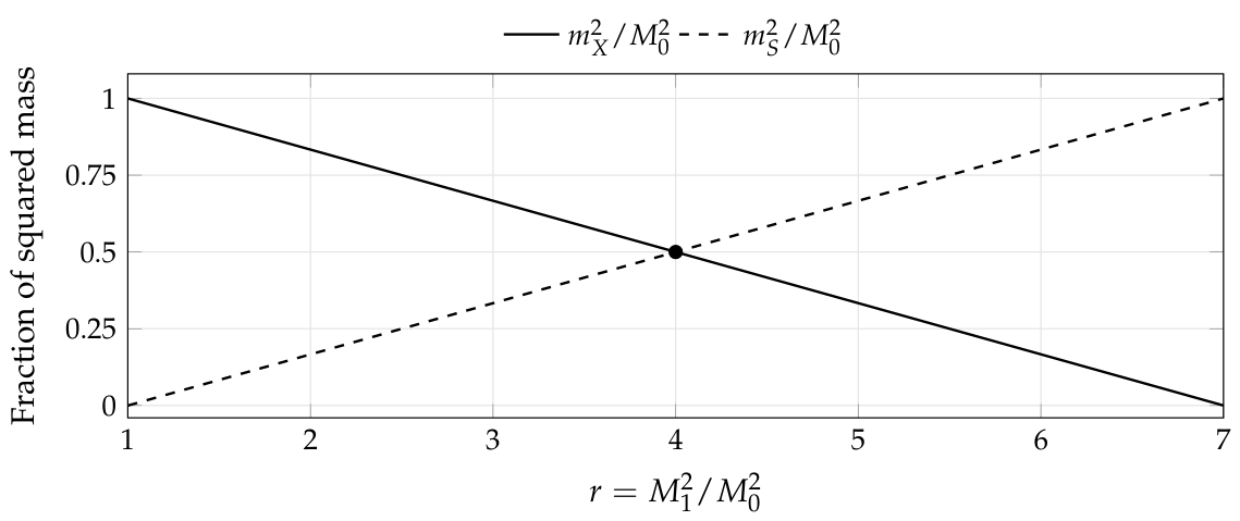
The scales are equal at $r=4$, the local mass term vanishes at $r=7$, and the relative observation contribution tends to zero as $r\downarrow 1$. These are contributions to the squared mass; $M_0$ itself is not the sum of the two scales.

In the chosen FS normalization, the length scale is also determined:

$$L_S={\displaystyle \frac{\sqrt{2}\hslash }{c{m}_S}}={\displaystyle \frac{\sqrt{12}\hslash }{c\sqrt{M_1^2-M_0^2}}}.$$

(70)

The quantity $m_S^2$ depends on the product of the lowest eigenvalue and the gradient coefficient. It is therefore invariant under the simultaneous rescaling described in the preceding section, as are the mass reconstruction formulas.

Figure 3. The squared-mass ratio of the two lowest levels fixes the relative contributions. The scales are equal at $r=4$. The limit $r\downarrow 1$ corresponds to $m_S/M_0\to 0$; if $M_0$ is held fixed, then $m_S\to 0$. The endpoint $r=1$ lies outside the parameter domain $m_S>0$.

Figure 3. The squared-mass ratio of the two lowest levels fixes the relative contributions. The scales are equal at $r=4$. The limit $r\downarrow 1$ corresponds to $m_S/M_0\to 0$; if $M_0$ is held fixed, then $m_S\to 0$. The endpoint $r=1$ lies outside the parameter domain $m_S>0$.

9.2. Parameter-Free Relations for Higher Levels

Eliminating $m_X$ and $m_S$ expresses every mass level in terms of $M_0$ and $M_1$:

$$M_n^2=M_0^2+{\displaystyle \frac{n(n+2)}{3}}(M_1^2-M_0^2),{\displaystyle \frac{M_n^2}{M_0^2}}=1+{\displaystyle \frac{r-1}{3}}n(n+2).$$

(71)

Once the first two levels have fixed the scales, the higher levels introduce no further mass parameters. The first two constraints are

$$3M_2^2=8M_1^2-5M_0^2,M_3^2=5M_1^2-4M_0^2.$$

(72)

Consecutive squared-mass gaps satisfy

$$(M_1^2-M_0^2):(M_2^2-M_1^2):(M_3^2-M_2^2)=3:5:7.$$

(73)

The corresponding ratio for a neutral field is $1:2:3$. The two gap laws arise from different phase representations and thus provide conditional tests for distinguishing the $q=0$ and $\left|q\right|=1$ spectra.

A spectral test first requires an identification of the levels. The masses being compared must belong to the same joint field and be consistent with its phase transformation law, degeneracies, and consecutive level assignments. The free action determines the propagation spectrum; preparation probabilities, detection strengths, and transitions between levels require interactions. An experimental test must therefore establish the observation geometry and phase transport, identify the two lowest distinct levels, and compare the subsequent spectral relations.

The geometry leaves one continuous freedom. Replacing $m_X^2$ by any other nonnegative constant preserves Lorentz symmetry, phase gauge covariance, and the $SU\left(2\right)$ symmetry of the observation sphere, without changing the line-bundle Chern number or ${\mathcal{K}}_q$. These geometric conditions fix the level coefficients but do not select a unique $m_X/m_S$. Fixing that ratio within the theory requires an additional dynamical condition on the local mass term.

9.3. A Necessary and Sufficient Condition for Equal Mass Spacing

The continuous freedom in the scale ratio is directly reflected in the shape of the spectrum. With $\eta =m_X^2/m_S^2$, completing the square in Eq. (65) gives

$$M_n^2=2m_S^2{(n+1)}^2+(m_X^2-m_S^2),{\displaystyle \frac{M_n^2}{M_0^2}}={\displaystyle \frac{\eta +2{(n+1)}^2-1}{\eta +1}}.$$

(74)

At the boundary $m_X=0$, the normalized squared masses are $1,7,17,31,\dots$. At $m_X=m_S$, the constant remainder vanishes and the masses themselves form an equally spaced sequence.

Proposition 9.2

(Equal-spacing criterion). Under the assumptions of Theorem 9.1, the mass spectrum has equal consecutive gaps if and only if $m_X=m_S$. In this case $r=4$, and

$$M_n=(n+1)M_0,M_0=\sqrt{2}{m}_S,E_{0,n}=(n+1)M_0{c}^2.$$

(75)

For arbitrary allowed scales, the second finite difference satisfies

$$sgn(M_{n+2}-2M_{n+1}+M_n)=sgn(m_X^2-m_S^2).$$

(76)

Proof. 

Set $B=m_X^2-m_S^2$ and $f\left(x\right)=\sqrt{2m_S^2{x}^2+B}$ for $x\ge 1$. The radicand is strictly positive, and

$$f^{\prime \prime }\left(x\right)={\displaystyle \frac{2m_S^{2}B}{{(2m_S^2{x}^2+B)}^{3/2}}}.$$

(77)

The second finite difference can be written as

$$M_{n+2}-2M_{n+1}+M_n={\int }_0^1{\int }_0^1{f}^{\prime \prime }(n+1+u+v)\mathrm{d}u\mathrm{d}v.$$

(78)

The integrand has the sign of B everywhere, proving Eq. (76). The finite difference vanishes if and only if $B=0$, in which case $f\left(x\right)=\sqrt{2}{m}_{S}x$ and the mass spectrum is equally spaced. □

The consecutive mass gaps therefore decrease when $m_X<m_S$ and increase when $m_X>m_S$, with $m_X=m_S$ separating the two behaviors. Exact equal spacing of any three identified consecutive levels suffices to determine this special parameter value. For every finite scale ratio, however, the gaps at high levels tend to $\sqrt{2}{m}_S$; approximate equal spacing at high levels does not have the same discriminating power. Equal spacing is a spectral selection condition. In this model, the dual-axis structure itself supplies no symmetry that exchanges the two axes and enforces $m_X=m_S$.

10. Physical Interpretation and Scope

10.1. The Mass of a Joint Excitation and Its Energy–Momentum Tensor

Mass belongs to the excitations of the joint field. The observation coordinate s labels the field’s internal geometric dependence, whose covariant gradient energy becomes a four-dimensional mass term after spectral decomposition. In the $\left|q\right|=1$ representation, $m_X^2$ and $[2n(n+2)+1]m_S^2$ are two contributions to the squared mass at level n; both belong to the complete mode at that level.

To examine gravitational coupling, we place the mode action (49) in a general spacetime metric $g_{\mu \nu }$ while holding the observation background fixed. This follows the proposed extension to relativistic dynamics in the PODA foundations [4], with the specific choice of minimal metric coupling. For a fixed mode, suppressing its degeneracy index, metric variation gives

$$\begin{array}{cc}\hfill T_{\mu \nu }^{\left(n\right)}=C_{\Psi }[& {\hslash }^2({\nabla }_{\mu }{\varphi }_n^{*}{\nabla }_{\nu }{\varphi }_n+{\nabla }_{\nu }{\varphi }_n^{*}{\nabla }_{\mu }{\varphi }_n)\hfill \\ \hfill & -g_{\mu \nu }\left({\hslash }^2{\nabla }_{\alpha }{\varphi }_n^{*}{\nabla }^{\alpha }{\varphi }_n-M_n^2{c}^2{\left|{\varphi }_n\right|}^2\right)].\hfill \end{array}$$

(79)

Here $y^0=ct$, the action measure is ${\mathrm{d}}^{4}y\sqrt{-g}/c$, and $T_{00}$ is the energy density in a local inertial frame. The mass contribution from observation gradients enters the energy–momentum tensor as part of the complete mode. The mass potential term alone does not, in general, define a separately conserved tensor.

On a prescribed flat background, the spatially uniform complex field

$${\varphi }_n\left(t\right)=a{e}^{-i{M}_n{c}^{2}t/\hslash }$$

(80)

solves the free-field equation. Equation (79) then gives

$$\epsilon =T_{00}=2C_{\Psi }{M}_n^2{c}^2{\left|a\right|}^2,P=0.$$

(81)

The corresponding mass density is $\epsilon /c^2$. This solution exhibits pressureless behavior of the complete mode on the given flat background; it has not been obtained by solving the field and gravitational equations self-consistently.

A connection to dark matter phenomenology also depends on the production, lifetime, momentum distribution, and detection couplings of the modes. Their cosmological abundance, role in structure formation, and gravitational effects can be calculated only once those conditions are specified. The mass spectrum and minimal metric coupling provide a field-theoretic starting point for such calculations. They do not by themselves identify dark matter or establish a new law of gravity.

10.2. Correlation Constraints and Spectral Tests

Event geometry and the covariant spectrum use the same observation space but govern different physical quantities. The former constrains probability correlations for a fixed prepared state; the latter determines the propagation levels of a joint field through the specified action. As long as observations of any additional modes retain Born pairing, the local binary spectral constraints, and the bipartite composition structure, the CHSH value continues to satisfy $|S_{\mathrm{CHSH}}|\le 2\sqrt{2}$.

Comparisons of higher-dimensional correlations test restrictions on state support and projection rank within the chosen quantum representation; the results are compatible with ordinary quantum theory. The mass relations instead test the free dynamics, full Hopf background, and phase representation adopted here. Their use of a common observation space does not make either set of results a consequence of the other. Both require a consistent distinction between physical states, observation structures, and the dynamical assumptions imposed on them.

11. Conclusion

The universal CHSH bound is fixed by the real Gram structure of Born pairing, with saturation attained in a two-dimensional plane. Enlarging the observation space leaves $2\sqrt{2}$ unchanged, while altering the event families available for a fixed prepared state. For a maximally entangled state uniformly occupying a d-dimensional Schmidt support, binary projections of arbitrary rank yield an attainable bound that depends on the parity of d; restricting the projections to rank one makes the excess over the classical bound decay as $1/d$. For the same state ${\Phi }_4$, the optimum can therefore rise from $1+\sqrt{2}$ to $2\sqrt{2}$. This difference reflects the measurement freedom allowed by projection rank and can be tested by comparing measurements while keeping the prepared state fixed.

In the joint-field action adopted here, positive gradient energy along the observation directions contributes to the masses of four-dimensional modes. The spectrum at the minimal nonzero phase weight, obtained from the standard ${\mathbb{CP}}^1$ metric and Hopf connection, gives

$$M_n^2=m_X^2+\left[2n(n+2)+1\right]m_S^2,E_{0,n}=M_n{c}^2.$$

(82)

The two lowest distinct mass levels determine the local mass parameter $m_X$ and the observation-gradient scale $m_S$, after which spectral relations constrain all higher levels without additional parameters. The second finite difference of the masses determines which scale is larger; exact equal spacing occurs uniquely at $m_X=m_S$. This equality is selected by a spectral condition. The continuous freedom in the local mass term prevents it from being a universal ratio fixed by the geometry.

A physical test of the mass spectrum requires the identification of different levels of the same joint field and the specification of their preparation and detection couplings. Under the chosen minimal metric coupling, observation-gradient energy contributes to the gravitational source through the energy–momentum tensor of the complete field. Its cosmological role further depends on the production, stability, and evolution of the modes. Regardless of how these dynamical modes are realized, the universal CHSH bound remains unchanged whenever their event statistics satisfy the Born representation and local binary constraints used here. Observation geometry can thus affect the propagation spectrum while preserving the dimension independence of the correlation bound.

References

- X. Meng, From Primitive Observation Records to the Dual-Axis Axiom: Set-Theoretic Foundations of Observational Geometry, Preprints.org, 2026081046, version 1 (2026). [CrossRef]
- X. Meng, Mathematical and Theoretical Foundations of the Basic Phase-Transport Equation: A Unified Differential, Covariant, and Path-Functional Theory, Preprints.org, 2026081128, version 1 (2026). [CrossRef]
- X. Meng, Quantum Correlations and the Tsirelson Bound in the Physical–Observation Dual-Axis Structure: From the Physobser Axiom, U(1) Phase Transport, and Composition Rules to the CP1 Observation Fiber and Born Probability Pairing, unpublished manuscript, revision R3.1, September 2026 (in Chinese).
- X. Meng, The Natural Dual-Axis Structure of Observation: Categorical Foundations and Consequences for Quantum Theory, unpublished manuscript, revised 5 September 2026.
- Maxwell, J. C. A dynamical theory of the electromagnetic field. Philosophical Transactions of the Royal Society of London 155, 459–512 (1865). [CrossRef]
- Einstein, A. Über einen die Erzeugung und Verwandlung des Lichtes betreffenden heuristischen Gesichtspunkt. Annalen der Physik 17, 132–148 (1905). [CrossRef]
- Einstein, A. Zur Elektrodynamik bewegter Körper. Annalen der Physik 17, 891–921 (1905). [CrossRef]
- Hehl, F. W. & Obukhov, Y. N. Foundations of Classical Electrodynamics: Charge, Flux, and Metric. Birkhäuser, Boston (2003).
- Meng, X. From primitive observation records to the dual-axis axiom: set-theoretic foundations of observational geometry. ResearchGate Preprint (2026). [CrossRef]