

Submitted:
24 September 2026
Posted:
28 September 2026
You are already at the latest version
Abstract
Deep learning has substantially advanced vibration-based fault diagnosis of rolling bearings, yet two obstacles continue to impede industrial deployment: the performance degradation that models suffer when transferred across test rigs (domain shift), and the scarcity of labeled fault data for newly commissioned machinery. This paper first establishes a unified, leakage-aware, multi-seed benchmark that spans three datasets (CWRU, Paderborn (PU) and SEU), all six cross-dataset transfer directions and eight modern baseline architectures, and subsequently proposes MLBA-Net, a lightweight hybrid network tailored to the extreme few-shot cross-domain scenario. MLBA-Net transforms vibration segments into three-channel continuous wavelet transform (CWT) images, extracts local time–frequency patterns through a convolutional stem, reorganizes the feature maps into frequency-band tokens that preserve the ordered harmonic structure of bearing fault signatures, and models them with a gated parallel bidirectional Mamba and bidirectional LSTM pair, followed by band attention and a multi-query pooling head. With merely 0.549 M parameters, MLBA-Net attains 98.26±0.43% accuracy on CWRU over ten seeds. In the central 1-shot CWRU→PU experiment it reaches a group Macro-F1 of 0.321±0.068—significantly ahead of both pure state-space models and the CNN baseline PFFNet, statistically tied with TimesNet, while trailing the two Transformer baselines—and it achieves the best zero-shot transfer in both PU-source reverse directions. The pure Mamba architecture fine-tunes worst of all models at every shot count, whereas the hybrid escapes this failure mode, suggesting that complementary inductive biases may improve adaptation stability under extremely limited target-domain supervision. Controlled studies further show that noise-augmented training, rather than an architectural denoising module, drives noise robustness, and that replacing the Mamba branch with a BiGRU yields statistically equivalent few-shot performance—an honest boundary on the architecture’s claims.
Keywords:
rolling bearing
; fault diagnosis
; Mamba
; long short-term memory
; attention mechanism
; cross-domain generalization
; few-shot learning
; transfer learning
; continuous wavelet transform
1. Introduction
Rolling bearings are ubiquitous in rotating machinery and are simultaneously among its most failure-prone components; undetected bearing degradation is a leading cause of unplanned downtime in motors, gearboxes, pumps and wind turbines [1]. Vibration-based condition monitoring, combined with deep learning, has therefore become the mainstream technical route for intelligent fault diagnosis, and benchmark accuracies on the Case Western Reserve University (CWRU) bearing dataset have been pushed close to saturation by convolutional neural networks (CNNs) [2,3], Transformer variants [4,5] and, most recently, state-space models (SSMs) exemplified by Mamba [6,7].
Nevertheless, a growing body of evidence indicates that in-domain benchmark performance is a poor proxy for deployability. A diagnostic model trained on one test rig is routinely confronted, in the field, with different bearing geometries, sampling rates, operating conditions and fault morphologies, under which its decision boundaries—partially fitted to dataset-specific spectral templates—may deteriorate to near-random levels. In the zero-shot experiments of this paper (Section 3.9, Section 3.11 and Section 3.12), all nine evaluated architectures attain merely 23–50% fault-type accuracy when transferred from CWRU to the Paderborn (PU) dataset without any adaptation, and zero-shot Macro-F1 values of merely 0.075–0.353 when transferred from CWRU to the SEU dataset, notwithstanding in-domain accuracies above 98%. Because labeling large volumes of vibration data for every newly deployed machine is economically impractical, cross-domain adaptation with only a handful of labeled samples per class, i.e., few-shot fine-tuning, constitutes the setting of genuine engineering relevance. We note explicitly that all three datasets used here are laboratory datasets; laboratory-to-laboratory transfer is a necessary intermediate step toward, but not a substitute for, laboratory-to-industrial validation.
A second, less explored question concerns the choice of architectural inductive bias under such regimes. CNNs hard-wire translation locality; Transformers relax structural priors in favor of global attention; SSMs impose sequential recurrence with linear-time complexity. Our systematic comparison reveals that these priors trade off differently across regimes: no single family dominates in-domain accuracy, zero-shot transfer, few-shot adaptation and noise robustness simultaneously, and the ranking in one regime fails to predict the ranking in another. Particularly noteworthy is the finding that pure Mamba architectures—despite their celebrated long-range modeling capacity—fine-tune unstably and rank last in the few-shot setting at every shot count, whereas recurrent (LSTM) and convolutional priors remain comparatively stable.
Motivated by these observations, we argue that the appropriate design for extreme few-shot cross-domain diagnosis is not the maximization of any single prior, but the complementary composition of several: local time–frequency extraction by convolutions, long-range selective memory by Mamba, local sequential bias by LSTM, and global band interaction by attention, together with a physically meaningful tokenization that respects the harmonic structure of bearing fault signatures.
The contributions of this paper are summarized as follows. (1) We establish a reproducible unified comparison framework covering three bearing datasets (CWRU, PU and SEU), all six cross-dataset transfer directions, eight baseline architectures together with the proposed model and four evaluation regimes (in-domain, zero-shot, few-shot, noisy), with ten random seeds, leakage-aware contiguous splits and paired bootstrap plus Wilcoxon signed-rank statistics throughout. (2) We propose MLBA-Net, a lightweight CNN–Mamba–LSTM hybrid with frequency-band attention (0.549 M parameters), which is competitive in the extreme few-shot regime: at 1-shot CWRU→PU it significantly outperforms both pure state-space models and the strongest CNN baseline, and it attains the best zero-shot transfer in both PU-source reverse directions. (3) We provide multi-seed empirical evidence that pure Mamba architectures fine-tune unstably under few-shot domain adaptation, and we report two informative negative results: the learnable fusion gate provides no statistically significant benefit over fixed gates, and replacing the Mamba branch with a BiGRU yields equivalent few-shot performance—evidence that the hybrid composition, rather than any specific component, carries the transfer behavior. (4) Through a controlled 2×2 study and fair retraining of all models, we show that noise-augmented training is the decisive factor for noise robustness, and we honestly report that CNNs, not the proposed model, remain strongest at low SNR.
We position the novelty of this work at three distinct levels. Architecturally, MLBA-Net contributes a specific, previously untested combination: frequency-band tokenization, gated parallel bidirectional Mamba/BiLSTM modeling and multi-query attention pooling in a sub-million-parameter design. Methodologically, the paper contributes a unified leakage-aware multi-seed evaluation protocol that, to the authors’ knowledge, is the first in this field to cover three datasets and all six transfer directions with paired statistical testing. Empirically, the paper contributes regime-resolved evidence of how modern architecture families behave under zero-shot, extreme few-shot and noisy conditions—including several findings that contradict our own earlier single-seed conclusions. We consider the second and third contributions at least as important as the architecture itself, and we have revised the manuscript throughout to claim no more than the multi-seed evidence supports.
2. Related Work
2.1. Deep Learning for Bearing Fault Diagnosis
Convolutional neural networks established the modern paradigm of vibration-based diagnosis after WDCNN demonstrated end-to-end classification from raw signals with explicit anti-noise and domain-adaptation design [8]. Residual learning [9] subsequently made deeper backbones trainable, squeeze-and-excitation re-weighting [10] became a standard capacity add-on, and diagnosis-specific innovations followed: deep residual shrinkage networks embed soft-threshold denoising into residual blocks for noisy conditions [3], and pyramid feature fusion designs such as PFFNet pursue robust multi-scale representation under small-sample conditions. These works delivered strong in-domain benchmarks, yet they are almost universally evaluated on a single dataset, with a single protocol, and frequently with a single random seed.
2.2. Transformers and Time-Series Models
Since the advent of attention [11], hierarchical vision Transformers such as Swin [5] have become strong generic backbones, while the time-series community has produced task-oriented variants: TimesNet folds one-dimensional sequences into two-dimensional period maps for general temporal analysis [12], and iTransformer inverts attention onto variate tokens, achieving state-of-the-art forecasting with remarkable simplicity [4]. Adapting these models to vibration time–frequency images is increasingly common; however, the adaptation itself—what should constitute a token, and which physical structure it should preserve—is seldom analyzed, and our results show that this choice alone can decide cross-domain success or failure.
2.3. State-Space Models and Mamba
State-space models culminating in Mamba offer selective, input-dependent sequence modeling with linear-time complexity [6], and have been rapidly transplanted to vision through bidirectional variants such as Vision Mamba [7] and native 2D designs such as Mamba-2D. In the diagnostic context, a hybrid of denoising multi-channel CNN mixture with Mamba-enhanced adaptive self-attention LSTM has recently demonstrated the promise of combining SSM with recurrent and attention mechanisms [13]. What remains unquantified is the behavior of pure SSM architectures under domain shift, few-shot adaptation and strong noise—regimes in which our experiments expose systematic weaknesses, including the worst few-shot fine-tuning among all evaluated architectures at every shot count.
A protocol-adapted reimplementation of this architecture under our unified benchmark (Section 3.17) confirms its strength at moderate shot counts and its inferiority to the proposed MLBA-Net in the extreme few-shot regime (1-shot F1: 0.274±0.030 vs. 0.321±0.068, n=10; paired difference +0.048, p=0.065).
2.4. Cross-Domain and Few-Shot Fault Diagnosis
Transferability has been pursued mainly through domain adaptation: deep adaptation networks align feature distributions via maximum mean discrepancy [14], and domain-adversarial training learns features that fool a domain classifier [15]; anti-noise and domain-adaptive ability were already joint design goals in WDCNN [8]. Beyond these, the wider literature offers several complementary routes that a practitioner may consider: domain generalization, which trains on multiple source domains to avoid target data altogether; self-supervised and contrastive pretraining, which exploits unlabeled target-domain signals [16]; meta-learning [17] and metric-based prototypical networks [18], which optimize directly for fast adaptation; and source-free domain adaptation, which adapts a source model without accessing the source data [19]. Each route makes assumptions that the present benchmark deliberately avoids: domain-adversarial and MMD-based methods require substantial unlabeled target data and careful optimization, meta-learning requires episodic access to related tasks, and source-free methods typically assume a well-behaved source classifier. Our study instead isolates the minimal commissioning scenario—one archived source model and a handful of labeled target segments—and asks which architectural priors survive it, leaving the systematic comparison of adaptation algorithms on top of this benchmark to future work.
Cross-dataset evaluation (e.g., CWRU→PU) is increasingly cited as evidence of generalization, yet protocols vary widely in label mapping, resampling and split hygiene, and single-seed results remain the norm. Table 1 positions representative studies along the dimensions that matter for the present claims; to the authors’ knowledge, few studies have systematically compared modern architecture families across datasets, transfer directions and regimes under a unified multi-seed protocol.
2.5. Noise-Robust Diagnosis
Robustness to additive noise is conventionally pursued through architectural denoising—most notably soft-threshold shrinkage modules embedded in residual networks [3]—or through training-side augmentation with synthetic noise. Our controlled 2×2 comparison (Section 3.14) adds quantitative evidence to an emerging view: the training protocol exerts a larger influence on noise robustness than the choice of architectural remedy, a finding with direct implications for how robustness claims should be benchmarked.
Positioning this work against the literature reveals three gaps: (i) few unified, multi-seed comparisons simultaneously cover in-domain, zero-shot transfer, few-shot adaptation and noisy regimes across modern architecture families, and none we are aware of covers three datasets in all six transfer directions; (ii) the few-shot and noise weaknesses of pure state-space models have not been quantified under paired statistical testing; and (iii) a hybrid design composing complementary inductive biases has not been tested in the extreme few-shot cross-domain regime that industrial commissioning approximates. These gaps define the contribution of the present paper.
3. Methodology and Experiments
3.1. Overall Framework
The overall architecture of MLBA-Net is illustrated in Figure 1, and the detailed structure of its core gated Mamba–BiLSTM frequency-band module is shown in Figure 2. A three-channel time–frequency image is processed through five cascaded stages: (i) a convolutional stem that extracts local time–frequency features while preserving the physically meaningful frequency axis; (ii) frequency-band tokenization, which converts the feature map into a short sequence of band tokens; (iii) a parallel bidirectional Mamba branch and bidirectional LSTM branch whose outputs are merged by a learned element-wise gate; (iv) frequency-band self-attention followed by a feed-forward network and squeeze-and-excitation re-weighting; and (v) a multi-query attention pooling head producing class logits. Each stage addresses a specific deficiency identified in our baseline analysis, and the design choices are ablated under ten seeds in Section 3.15. Module-level tensor shapes and parameter counts are given in Table 2; Algorithm 1 states the forward pass. Operator-level factorization (every convolution, the internal MambaSSM scan, and the classifier) is deferred to Appendix A (Table A1) so that the main text can argue for the design rather than enumerate layers.
Table 2 reports every learnable module, its output tensor and its parameter count, measured on the implemented model (548,874 trainable parameters). Algorithm 1 is the corresponding forward computation. Equations in Section 3.2, Section 3.3, Section 3.4 and Section 3.5 detail only the operators that differ from a standard CNN–RNN hybrid; CWT, selective-scan discretization and multi-head attention otherwise follow their usual definitions.
| Algorithm 1. Forward pass of MLBA-Net. | ||
| Step | Computation | |
| Input | X ∈ R^{B×3×32×32} (three-channel CWT image) | |
| 1 | H ← Stem(X) | ▷ 4×3×3 conv, H ∈ R^{B×64×16×16} |
| 2 | Z ← BandTokenize(H) + E_band | ▷ Z ∈ R^{B×16×128} |
| 3 | y_m ← ½ [ SSM(Z) + flip(SSM(flip(Z))) ] | ▷ shared weights |
| 4 | y_l ← BiLSTM(Z) | |
| 5 | g ← σ(W_g [y_m ; y_l] + b_g) | |
| 6 | h ← LN( g ⊙ y_m + (1−g) ⊙ y_l + Z ) | |
| 7 | h ← LN( h + MHA(h) ) | ▷ 8 heads |
| 8 | h ← LN( h + FFN(h) ) | ▷ 128→256→128 |
| 9 | h ← h ⊙ SE(mean_f(h)) | |
| 10 | P ← MultiQueryPool(h ; Q ∈ R^{4×128}) | ▷ P ∈ R^{B×512} |
| Output | logits ← MLP(P) | ▷ 512→128→10 |
Each convolution is followed by batch normalization and ReLU. Dropout p=0.1 is applied after the token projection, inside the FFN and in the classifier. The bidirectional Mamba uses a single shared selective-scan module, not two independent SSMs. MHA denotes one attention block, not a stack of N Transformer layers.
3.2. Multi-Sensor Time–Frequency Image Input
Raw vibration signals are segmented into non-overlapping windows of 1024 samples and z-score normalized per segment to eliminate amplitude discrepancies arising from varying loads. Each segment is transformed by the continuous wavelet transform (CWT) with a Morlet mother wavelet at 32 scales [20] and resized to 32×32 pixels. CWT is preferred over the short-time Fourier transform for its superior time–frequency localization of transient impulses characteristic of incipient bearing faults. The three input channels correspond to the drive-end (DE), fan-end (FE) and base (BA) accelerometers, so that multi-sensor information is fused at the input level; the missing BA channel of the healthy class is replaced by DE. For the PU dataset (single accelerometer, 64 kHz), signals are resampled to 12 kHz and the single channel is replicated three times, ensuring identical input shapes across datasets and models. For the SEU dataset, the three planetary-gearbox vibration channels (x/y/z) form a genuine three-channel input, and a replicated single-channel variant is constructed for the sensor-configuration isolation experiment (Section 3.13). Section 3.13 quantifies how much of the measured domain shift is attributable to this sensor-configuration mismatch rather than to genuine rig and fault differences.
Formally, the input construction is:
3.3. CNN Stem and Frequency-Band Tokenization
As shown in Figure 1 and Table 2, a four-layer 3×3 convolutional stem (32→32→64→64 channels, with one stride-2 downsampling to 16×16) first extracts local time–frequency patterns; batch normalization and ReLU follow each convolution. Only the third layer downsamples, which aligns the frequency axis with 16 band tokens without the deeper stem that overfits the source domain (Section 3.15). The resulting 64×16×16 feature map is then sliced along the frequency axis: each of the 16 frequency bands becomes one token of 64×16 = 1024 dimensions, which is linearly projected to d_model = 128 and augmented with a learnable band position embedding. This tokenization is physically motivated—fault characteristic frequencies and their harmonics form an ordered progression along the frequency axis—and it stands in deliberate contrast to patch-flattened tokenization (as adopted in VisionMamba), which our experiments demonstrate to generalize poorly across domains (Section 3.9).
Formally, the stem and tokenization are:
3.4. Bidirectional Mamba ∥ BiLSTM Gated Fusion
The band-token sequence is modeled in parallel by two complementary branches (Figure 2). The bidirectional Mamba branch applies a shared selective-scan SSM [6] in both directions (implemented as a numerically stable pure-PyTorch chunked scan), capturing long-range selective memory along the harmonic axis; the bidirectional LSTM branch [21] supplies the well-understood local sequential bias and stable fine-tuning behavior of gated recurrent units. The branch outputs are fused element-wise with a learned gate: h = g⊙y_m + (1−g)⊙y_l + x, where g = σ(W[y_m; y_l]) and x denotes the branch input. The gate is interpretable: it quantifies, per feature, how much the model relies on SSM-based global memory versus recurrent local dynamics. While initially hypothesized to act as a domain-adaptive arbitrator (Section 4.3), we find that the network learns a stable, domain-invariant ensemble balance, and the multi-seed ablation (Section 3.15) further shows that fixed gates match or exceed the learnable gate under paired testing. The Mamba branch uses a single shared selective-scan module rather than two independent SSMs (Table 2); the backward pass is therefore a parameter-free flip–scan–flip average (Table A1). On the trained model the mean gate is domain-stable (0.461 on the CWRU test set, n=484; 0.466 on the PU evaluation pool, n=1440), consistent with the multi-seed measurements in Section 4.3.
The two branches and the fusion are defined as:
3.5. Frequency-Band Attention and Multi-Query Pooling
The fused tokens are further processed by a single multi-head self-attention layer (8 heads)—not a stack of Transformer encoders—that models global interactions between frequency bands, followed by a position-wise feed-forward network (128→256→128) and a squeeze-and-excitation block (reduction 4), each wrapped with residual connections and LayerNorm (Table 2). Classification employs four learnable queries that attention-pool the band tokens; the concatenated pooled vectors (4×128) are passed to a two-layer classification head (512→128→10). In contrast to global average pooling, the multi-query mechanism lets the classifier attend to several distinct fault-relevant bands simultaneously; the multi-seed ablation (Section 3.15) examines its contribution together with all other components.
The attention head is defined as:
3.6. Training and Evaluation Protocol
All models, baselines included, are trained under an identical protocol: Adam optimization (lr = 1e-4), batch size 64, at most 100 epochs with cosine annealing, early stopping (patience 20) monitored on validation Macro-F1, and cross-entropy loss. We deliberately do not perform per-model hyperparameter tuning: a single common configuration cannot be optimal for every architecture family, and we report this as a limitation (Section 4.8) rather than claim strict optimality for any baseline; the identical protocol at least guarantees that differences are attributable to the architectures under one fixed, disclosed budget. Unless stated otherwise, every experiment is repeated with ten random seeds (42–51) and reported as mean±SD; 95% confidence intervals and medians for the main experiments are compiled in Appendix Table A2, individual per-seed values are released with the result files (Data Availability Statement), and key paired comparisons—identical splits and seeds for both sides—with percentile bootstrap confidence intervals of the mean difference (10,000 resamples) and two-sided Wilcoxon signed-rank tests at α=0.05. To preclude leakage, splits are contiguous within each recording file (70/20/10 train/val/test) and windows never overlap; we acknowledge that adjacent segments of a quasi-stationary recording may still be correlated (Section 4.8). For cross-domain evaluation, classes are aligned to fault-type groups and predictions are mapped to the same groups before scoring (Section 3.7.1). Few-shot fine-tuning uses Adam (lr = 1e-5) for 50 epochs with k ∈ {1, 5, 10, 20} shots per class drawn from a support pool strictly disjoint from the evaluation pool. Noise robustness is assessed by training on clean signals and testing with additive white Gaussian noise at SNR ∈ {−4, −2, 0, 2, 4, 6, 8, 10} dB, with identical noise realizations shared across models (paired comparison); a fair variant retrains all models with noise augmentation (50% of training segments noised at random SNR ∈ [−4, 10] dB). The noise study, which originally predated the seed extension, has likewise been extended to the same ten seeds.
3.7. Experimental Setup
3.7.1. Datasets
CWRU [1]: ten classes from the 12 kHz drive-end recordings (normal; inner-/outer-race and ball faults of 0.007/0.014/0.021 inches at the 6 o’clock load zone), using the canonical file-number assignment. After class balancing, the splits contain 3353/951/484 train/validation/test segments. PU [22]: nine classes (one healthy K001; four artificial outer-race damages KA01/03/05/07; four artificial inner-race damages KI01/03/05/07), resampled from 64 kHz to 12 kHz, with 4320 support and 1440 evaluation segments. SEU [23]: the Southeast University gearbox bearing subset (bearingset), five classes (health, ball, comb, inner, outer) under two operating conditions (20 Hz–0 load and 30 Hz–2 load), resampled from 5.12 kHz to 12 kHz, with the three planetary-gearbox vibration channels (x/y/z) forming the genuine three-channel input; 256 segments per file yield 2560 samples, split contiguously 70/20/10 within each recording as for the other datasets. For cross-dataset alignment, classes are mapped to fault-type groups: CWRU and PU share {N, IR, OR} (PU contains no ball-damage category); SEU is aligned to {N, IR, B, OR} for CWRU/SEU transfers, with the compound-fault class comb excluded from cross-domain experiments because it has no counterpart group in CWRU or PU (retained for the SEU in-domain benchmark, which is therefore five-class). When PU serves as the source domain, its nine-class label space is used for training and only the shared groups {N, IR, OR} are evaluated on the targets. The three datasets differ in bearing type, test rig, sampling rate and damage genesis, and thus constitute a genuine cross-domain benchmark, though still a laboratory one.
3.7.2. Baselines and Implementation Details
Eight representative baselines are implemented under the same input and training protocol: PFFNet (reproduced from the paper description, featuring residual shrinkage and pyramid fusion), Swin-Transformer (timm swin_tiny adapted to 32×32 [24]), iTransformer (a re-implemented variate-attention classifier), ResNeSt-50d (timm, split-attention), Mamba-2D and VisionMamba (pure-PyTorch selective scan, since mamba-ssm is unavailable on Windows), TimesNet (a re-implemented period-folding classifier), and a protocol-adapted reimplementation of the closest related architecture [13] (Section 3.17). All experiments run on a single RTX 4060 Laptop GPU (8 GB) with PyTorch 2.5.1+cu121; the full codebase, caches, seeds, per-seed metrics and logs are retained for reproducibility.
3.8. In-Domain Comparison on CWRU
The CWRU benchmark proves to be saturated: the four leading models span merely 99.34–99.57%, and per-class errors in the confusion matrix are essentially absent (Figure 3). MLBA-Net ranks sixth at 98.26±0.43%, and the paired tests quantify the gap honestly: it trails the top tier (iTransformer by 1.09 points, 95% CI [0.75, 1.50], p=0.002; ResNeSt by 1.27, p=0.002; PFFNet by 1.31, p=0.002) while leading TimesNet by 8.86 points (p=0.002), at merely 0.549 M parameters—46× fewer than ResNeSt—and 3.52 ms per-sample inference. It is worth emphasizing that single-seed 100% accuracies occasionally reported in the literature did not survive multi-seed scrutiny (iTransformer measures 99.34±0.27% over ten seeds), underscoring the necessity of mean±SD reporting on saturated benchmarks.

Table 3.
In-domain results on CWRU (mean±SD, n=10 seeds).
| Model | ACC (%) | Macro-F1 (%) | Macro-AUC | Params (M) | FLOPs (G) | Infer. (ms) |
| PFFNet | 99.57±0.15 | 99.56±0.15 | 1.000±0.000 | 1.82 | 0.467 | 3.93 |
| Swin-Transformer | 98.68±0.58 | 98.66±0.59 | 1.000±0.000 | 27.51 | 0.356 | 9.14 |
| iTransformer | 99.34±0.27 | 99.33±0.27 | 1.000±0.000 | 0.32 | 0.005 | 0.86 |
| ResNeSt | 99.52±0.26 | 99.52±0.26 | 1.000±0.000 | 25.45 | 1.684 | 11.96 |
| Mamba-2D | 98.47±0.50 | 98.46±0.51 | 1.000±0.000 | 0.12 | 0.012 | 8.16 |
| VisionMamba | 94.55±2.34 | 94.43±2.41 | 0.996±0.002 | 0.13 | 0.008 | 8.07 |
| TimesNet | 89.77±1.87 | 89.39±2.31 | 0.989±0.008 | 9.38 | 4.499 | 10.84 |
| Sensors-MASA | 98.20±0.54 | 98.18±0.55 | 0.999±0.001 | 0.281 | — | — |
| MLBA-Net (ours) | 98.26±0.43 | 98.25±0.44 | 1.000±0.000 | 0.549 | 0.030 | 3.52 |
3.9. Zero-Shot Cross-Domain Evaluation on PU
Zero-shot transfer is uniformly difficult: every architecture scores between 23% and 50% group accuracy against a 33% random baseline, confirming a substantial domain gap between the two rigs in bearing geometry, sampling and damage morphology. The seed-to-seed variance remains striking (up to ±9.3 percentage points for VisionMamba), which cautions against interpreting single-seed transfer rankings that are common in the literature. Two findings prove robust across ten seeds: iTransformer’s group accuracy (49.58±3.35%) and Macro-F1 (0.323±0.035), attributable to its minimal inductive bias and LayerNorm-based design, and Mamba-2D’s second-best Macro-F1 (0.295±0.065). MLBA-Net is mid-pack before adaptation (0.259±0.052; statistically tied with ResNeSt, p=0.63, and PFFNet, p=0.77, and behind iTransformer, p=0.002)—a point we return to in Section 4.1: the model is designed for few-shot domain adaptation, not for domain generalization, and we do not claim zero-shot competence for it in this direction. The confusion matrix (Figure 4) shows that mild outer-race damage (KA01) transfers best, whereas mild inner-race damage (KI01) is almost universally missed—a pattern shared by all evaluated models.
Table 4.
Zero-shot CWRU→PU transfer at fault-type group level {N, IR, OR} (mean±SD, n=10).
| Model | Group ACC (%) | Group Macro-F1 |
| PFFNet | 34.41±7.99 | 0.259±0.078 |
| Swin-Transformer | 37.12±4.46 | 0.254±0.026 |
| iTransformer | 49.58±3.35 | 0.323±0.035 |
| ResNeSt | 29.36±7.39 | 0.266±0.088 |
| Mamba-2D | 43.19±3.68 | 0.295±0.065 |
| VisionMamba | 23.28±9.26 | 0.162±0.046 |
| TimesNet | 38.61±6.21 | 0.183±0.020 |
| Sensors-MASA | 35.31±4.90 | 0.237±0.033 |
| MLBA-Net (ours) | 32.44±6.33 | 0.259±0.052 |
The per-class heatmap (Figure 5) resolves the aggregate numbers into a coherent physical pattern over the same ten seeds used throughout this study. Transfer accuracy is ordered by damage location and severity: mild outer-race damage induced by electrical discharge machining (KA01) transfers best for nearly every model (60–99% mean accuracy), and on average across models the artificial outer-race family remains markedly more transferable than the inner-race family; the mild inner-race damage KI01, by contrast, is nearly invisible to every architecture (0–10%), forming a uniform column of failure. This class-level gradient—rather than the averaged scores—defines the concrete obstacle that few-shot adaptation must overcome, and explains why even one labeled sample per class improves transfer markedly (Section 3.10).
3.10. Few-Shot Cross-Domain Fine-Tuning (Main Experiment)
The few-shot regime constitutes the central experiment of this study (Table 5, Figure 6a). At k = 1, MLBA-Net attains 0.321±0.068 Macro-F1 and ranks fourth of nine architectures. The paired analysis (Table 6) delineates this standing precisely: MLBA-Net is significantly ahead of both pure state-space models (Mamba-2D +0.077, p=0.027; VisionMamba +0.064, p=0.027) and of the CNN baseline PFFNet (+0.071, p=0.020), marginally ahead of ResNeSt (+0.042, p=0.064) and of the reimplemented Sensors-MASA (+0.048, p=0.065), statistically tied with TimesNet, and behind the two Transformer baselines (iTransformer −0.085, p=0.014; Swin −0.064, p=0.084). We state this standing transparently and claim only what the ten-seed evidence supports; how the three-seed-to-ten-seed extension revised our own earlier conclusions is examined in Section 4.5.
In stark contrast, Mamba-2D fine-tunes worst of all architectures at every shot count (0.244 at k=1, and merely 0.341 even at k=20—barely above its own zero-shot level), confirming over ten seeds that a pure selective-scan SSM is unstable to adapt from a handful of target-domain samples; the hybrid MLBA-Net, sharing the same SSM machinery yet augmented with LSTM and attention, escapes this failure mode entirely. At k=20, large-capacity CNNs eventually catch up (ResNeSt 0.690, p=0.004 against MLBA-Net), which delineates MLBA-Net’s operating sweet spot as the extreme few-shot regime (k ≈ 1) that is most relevant to industrial commissioning, rather than few-shot superiority in general.
3.11. Third-Dataset Validation on SEU
3.11.1. SEU In-Domain Benchmark
Unlike saturated CWRU, the five-class SEU benchmark remains discriminative (Table 7): iTransformer leads at 95.42±0.64%, followed by ResNeSt and Swin-Transformer, while MLBA-Net is mid-pack at 85.77±1.79% and VisionMamba trails at 74.65±4.39%. The spread of over 20 points between the best and worst architectures confirms that SEU provides a useful second in-domain reference in which design differences are not masked by ceiling effects.
3.11.2. CWRU→SEU Zero-Shot and Few-Shot Transfer
Transfer from CWRU to SEU is markedly harder than to PU (Table 8, Figure 6b): zero-shot Macro-F1 spans merely 0.075–0.353 against a 25% random baseline, and even at k=20 only Swin-Transformer (0.719) and ResNeSt (0.663) exceed 0.65. Two regime-dependence observations are noteworthy. First, TimesNet—mediocre on CWRU→PU—attains the best zero-shot transfer (0.353±0.026) yet saturates early, whereas Swin-Transformer starts poorly and ends first; no architecture dominates both ends of the curve. Second, iTransformer, the strongest zero-shot model toward PU, collapses almost completely toward SEU (0.075±0.028), demonstrating that its CWRU→PU robustness does not generalize across target domains—a further instance of rankings in one regime failing to predict another. MLBA-Net is again mid-pack (0.172 zero-shot, 0.507 at k=20), and we do not claim an advantage in this direction.
3.11.3. SEU Cross-Condition Transfer (Leave-One-Condition-Out)
To probe operating-condition shift—the leave-one-operating-condition-out validation requested by the reviewer—we trained on one SEU condition and evaluated on the other (Table 9). Cross-condition zero-shot transfer is far less severe than cross-dataset shift (Macro-F1 0.43–0.58), and five labeled samples per class lift most models to 0.60–0.79; ResNeSt and PFFNet are strongest in both directions. MLBA-Net behaves asymmetrically: competitive in the 20_0→30_2 direction (0.662 at k=5) but the weakest in the reverse direction (0.484 at k=5). Cross-condition transfer therefore remains an open difficulty for all evaluated architectures, and we report it as such rather than as a strength of the proposed model.
3.12. Reverse Transfer: Completing the Six Directions
3.12.1. SEU→CWRU and SEU→PU
With SEU as a four-class source (Table 10), transfer to CWRU is effective after adaptation—at k=20 ResNeSt reaches 0.916 and Swin-Transformer 0.902—whereas transfer to PU is harder for every model (best 0.565, Sensors-MASA). MLBA-Net is mid-pack in both directions (0.715 and 0.521 at k=20). The asymmetry is informative: the difficulty of a transfer direction depends jointly on the source label-space coverage and the target’s spectral similarity to the source, not on any single architecture property.
3.12.2. PU→CWRU and PU→SEU
When the nine-class PU dataset serves as the source (Table 11), MLBA-Net attains the best zero-shot transfer of all nine architectures in both directions—Macro-F1 0.307±0.092 toward CWRU and 0.253±0.060 toward SEU, with group accuracies of 42.62±7.44% and 34.50±3.47%—its clearest zero-shot result in the entire benchmark. We interpret this cautiously: the richer nine-class PU source exposes the model to a wider diversity of fault morphologies during pre-training, and MLBA-Net’s band-structured representation appears to exploit this diversity better than the alternatives; the advantage does not persist as the leading margin once target labels become available (at k=20, ResNeSt 0.973 and Swin 0.969 toward CWRU exceed MLBA-Net’s 0.898). PU→SEU is the most difficult of the six directions overall (best k=20 F1 0.720, ResNeSt), plausibly because PU’s artificial damage genesis transfers least to SEU’s run-to-failure-like wear. With Table 5 and Table 8, 10 and 11, all six transfer directions among the three datasets are now covered, and the direction-dependence of every architecture family is on record.
3.13. Sensor-Configuration Isolation
A legitimate concern with the CWRU→PU protocol is that CWRU uses three sensor channels while PU contributes a single accelerometer whose signal is replicated three times: part of the measured domain gap could stem from this sensor-configuration mismatch rather than from genuine bearing and rig differences. We therefore retrained five representative models on a channel-replicated CWRU input (DE×3) and evaluated them on PU (replicated) and on both SEU channel variants (Table 12). Three observations answer the concern. First, source-side channel form shifts transfer F1 by less than ≈0.05 in most cells (23 of 35), and the sign of the shift is inconsistent—PFFNet transfers slightly better from a replicated source on PU at k=1 (0.280 vs. 0.250), and even the genuine multi-sensor target SEU-multi at k=5 is reached better from a replicated source by ResNeSt (0.421 vs. 0.350) and PFFNet (0.368 vs. 0.317). Second, the largest gaps (up to ≈0.12, e.g., MLBA-Net toward replicated SEU at k=5: 0.298 multi vs. 0.174 rep) do not consistently favor either configuration—the same column contains a 0.052 gap of the opposite sign for ResNeSt (0.381 multi vs. 0.433 rep), and the sign flips across columns for four of the five models. Third, replication costs in-domain accuracy in all five models without exception (CWRU in-domain F1 drops by 0.8–3.5 points depending on the model), yet this in-domain penalty does not translate into a systematic transfer penalty. We conclude that the reported cross-dataset domain gap is dominated by genuine rig, bearing and fault-morphology differences rather than by the PU channel replication, while acknowledging the replicated-channel design as a residual limitation (Section 4.8).
3.14. Noise Robustness
Under the conventional clean-training protocol, the SSM family proves strikingly noise-sensitive: MLBA-Net attains an F1 of only 0.138 at −4 dB, and Mamba-2D and VisionMamba likewise occupy the bottom tier, whereas iTransformer (0.423) degrades most gracefully. A controlled 2×2 experiment—{v3.3 vs. +soft-threshold shrinkage} × {clean vs. noise-augmented training}—was conducted to disentangle architectural from training-side remedies. The shrinkage module, adapted from deep residual shrinkage networks [3], was decisively rejected (no consistent gain in either setting), whereas noise augmentation lifted MLBA-Net’s F1 at −4 dB from 0.138 to 0.679 (a 4.9× improvement) at a cost of only 1.7 points of clean accuracy.
Under the fair protocol in which every model is retrained with identical noise augmentation (Table 13, Figure 7), two honest conclusions emerge. First, noise-augmented training benefits all models substantially—TimesNet’s −4 dB F1 rises from 0.177 to 0.349, and similar gains are observed everywhere—indicating that the training protocol exerts a larger influence on noise robustness than architectural differences. Second, CNN baselines (ResNeSt 0.823, PFFNet 0.812 at −4 dB) remain strongest at low SNR, with MLBA-Net (0.679) mid-pack; we therefore do not claim noise robustness as a strength of the proposed model and instead report it as a delineated limitation. The noise experiments have since been extended to the same ten seeds (42–51) as the main experiments.
3.15. Multi-Seed Ablation Study
The multi-seed ablation (Table 14) replaces our earlier single-seed and three-seed ablations, which had suggested larger component effects; those effects did not survive seed extension, and we report the ten-seed picture plainly. In-domain, no variant differs significantly from base under paired testing (all |Δ| ≤ 0.34 points, n=10). At PU 1-shot, no variant is significantly worse than base either: removing the band attention is the only change that trends negative (−0.028 F1, n.s.; in-domain −0.34, p=0.064), while the Mamba-only (+0.023, n.s.) and fixed-gate variants (−0.001 to −0.002, n.s.) remain statistically tied with base. At 5-shot, several simplifications significantly outperform base: Mamba-only (+0.039, p=0.010), no-gate (+0.054, p=0.010), fixed gates (+0.048 to +0.056, p<0.05) and the BiGRU replacement (+0.062, p=0.002).
We draw three conclusions. First, MLBA-Net’s components form a redundant, robust composition rather than a chain of indispensable parts: the model degrades gracefully when any single module is removed, and the band-attention block is the only component whose removal consistently trends in the negative direction. Second, the learnable fusion gate does not survive multi-seed scrutiny—fixed gates match it at 1-shot and exceed it at 5-shot—consistent with the domain-stability measurement of Section 4.3; we retain the learnable gate in the reported model for interpretability (it exposes the branch balance directly), but we no longer claim it as a performance-critical component. Third, the Mamba branch itself is not necessary for the observed few-shot behavior: a size-matched BiGRU performs equivalently at 1-shot and better at 5-shot. Section 4.4 discusses what this implies for the architecture’s identity.
3.16. Complexity Evaluation
MLBA-Net comprises 0.549 M parameters and 0.030 GFLOPs per 32×32 input, infers in 3.52 ms per sample and trains to convergence in approximately one minute—an order of magnitude lighter than CNN baselines of comparable in-domain accuracy (ResNeSt: 25.45 M, 1.68 GFLOPs, 11.96 ms; 18.5 min training). We emphasize that these measurements were made on an RTX 4060 Laptop GPU, not on an industrial edge platform; the profile therefore supports only potential edge deployment in commissioning scenarios where only a few labeled samples are available, and on-device validation remains future work (Section 4.8).
3.17. Comparison with the Closest Related Architecture
To position MLBA-Net against the closest published architecture, we reimplemented the MOM-Conv + MASA-LSTM model of Sensors 2025, 25, 6652 [13] from the paper’s equations and evaluated it under the identical protocol. Because several adaptations were unavoidable, we describe this as a protocol-adapted reimplementation rather than a faithful reproduction: we replaced its denoised 2D-DFT image input with our standardized CWT input (A1); its 5-D MoE formulation is adapted to 4-D feature maps with the frequency axis as the token dimension (A2); four linear experts with top-2 gating are used (A3); the flattened sequence is pooled from 256 to 64 steps for tractable stepwise LSTM iteration (A4); the multi-head self-attention is applied once over the whole hidden sequence instead of per-step (A5); a mean-pooling linear head is used for classification (A6); and the Mamba branch uses the paper’s zero-order-hold discretization (A7).
Under ten seeds the two models are essentially tied in-domain (Δ = 0.06 points) and in zero-shot transfer (0.259 vs. 0.237). MLBA-Net’s advantage at 1-shot, which a three-seed evaluation had suggested was large, is revised to a marginal one (+0.048 F1, 95% CI [+0.010, +0.091], p=0.065); at k=20 the reimplementation reaches parity (0.561 vs. 0.550, p=1.0) with half the parameters, its stepwise gated LSTM cell paying off once more adaptation data is available. The component comparison (Table 16) attributes the remaining 1-shot margin primarily to the explicit frequency-band tokenization and multi-query pooling rather than to the sequence-modeling machinery, which the two models share conceptually.
Table 15.
Comparison with the protocol-adapted reimplementation of Sensors 2025 (mean±SD, n=10).
| Model | CWRU ACC (%) | CWRU F1 (%) | PU zero-shot F1 | 1-shot F1 | 5-shot F1 | 10-shot F1 | 20-shot F1 | Params (M) |
| MLBA-Net (ours) | 98.26±0.43 | 98.25±0.44 | 0.259±0.052 | 0.321±0.068 | 0.394±0.069 | 0.479±0.084 | 0.550±0.057 | 0.549 |
| Sensors-MASA (reimpl.) | 98.20±0.54 | 98.18±0.55 | 0.237±0.033 | 0.274±0.030 | 0.389±0.045 | 0.469±0.075 | 0.561±0.088 | 0.281 |
Table 16.
Component-level comparison with the Sensors 2025 architecture.
| Component | MLBA-Net (ours) | Sensors-MASA (reimpl.) |
| CNN front-end | 4-layer conv stack (32→64), no MoE | MOM-Conv: 4-branch standard/dilated convs + dual MoE (4 experts, top-2) + GAP-FC ⊙ pointwise sigmoid gate |
| Mamba implementation | Shared bidirectional SSM, chunked scan, simplified ΔB | External Mamba: 2 residual blocks + two-branch Mamba, ZOH discretization, stepwise scan |
| LSTM role | Parallel independent branch (BiLSTM) | Backbone: custom MASA-LSTM cell (two-previous hidden states, learnable α/β gate scaling) |
| Attention | Standard MHA (8 heads) over band tokens + FFN + SE | MSA over hidden-state sequence (4 heads) + residual + LN |
| Tokenization | Explicit frequency-band tokens (16×128-d) + position embedding | None: feature map flattened to a 64-step sequence |
| Fusion mechanism | Learnable element-wise gate g = σ(W[y_m;y_l]) + residual | Hadamard branch product; learnable α/β scalars in LSTM cell |
| Pooling/head | Multi-query attention pooling (4 queries) + 2-layer MLP | Mean over hidden states + Linear |
| Parameters | 0.549 M | 0.281 M |
4. Discussion
4.1. Why Pure State-Space Models Falter Under Noise and Few-Shot Adaptation
A consistent pattern across all regimes is the underperformance of pure SSM architectures outside their comfort zone, now established over ten seeds: Mamba-2D fine-tunes worst of all models at every shot count on CWRU→PU, and both pure SSMs occupy the bottom tier under low-SNR noise. We hypothesize that the selective-scan recurrence, which propagates a compressed hidden state along the sequence, accumulates broadband noise into that state: additive white noise corrupts every time step, and the recurrence offers no spatial averaging mechanism analogous to CNN pooling to cancel it. The same compression may explain poor few-shot fine-tuning—adaptation must travel through a low-dimensional bottleneck of learned state-transition parameters, whereas attention- and pooling-based heads expose more directly adjustable parameters to the few available gradients. That noise-augmented training restores much of the deficit (Section 3.14) supports this interpretation: once the state dynamics are explicitly exposed to noise during training, the scan learns to discount corrupted steps.
Two qualifications sharpen the picture. First, the instability is a property of the pure, patch-tokenized SSM architecture rather than of the selective-scan mechanism itself: MLBA-Net’s Mamba-only ablation variant—which retains the CNN stem, band tokenization and attention head—fine-tunes stably and matches or exceeds the full model (Section 3.15). The failure is therefore best attributed to the combination of patch tokenization and an unsupported SSM backbone, not to SSMs per se. Second, MLBA-Net’s mid-pack zero-shot standing on CWRU→PU should be read in light of the distinction between domain generalization and few-shot domain adaptation: the model is designed for the latter—becoming competitive with a handful of target labels—and we do not claim zero-shot domain-general competence for it. Notably, when the label-rich PU dataset serves as the source, MLBA-Net does attain the best zero-shot transfer of the benchmark in both target directions (Section 3.12.2), suggesting that its representation benefits more from source diversity than the alternatives; we report this as an observation, with its mechanism left to future work.
4.2. The Robustness of iTransformer Reconsidered
On CWRU→PU, iTransformer is the most robust baseline (best zero-shot and few-shot F1), and we attribute this to the conjunction of three properties rather than to any single one: its variate tokens expose entire spectral profiles to one-hop global comparison; its LayerNorm-based normalization avoids the batch-statistics mismatch that afflicts BatchNorm-based CNNs under domain shift; and its minimal inductive bias imposes no structural assumption—locality, order or periodicity—that domain shift could invalidate. This observation suggests that architectural prior should be viewed as a tunable liability whose cost is charged exactly when the deployment domain departs from the training domain.
The extended benchmark tempers this attribution with two further observations. First, iTransformer’s robustness is direction-specific: on CWRU→SEU it collapses to the worst zero-shot F1 of the field (0.075), so minimal inductive bias alone does not guarantee transfer when the target domain is sufficiently distant; LayerNorm and variate tokens appear to help specifically where the shift is moderate. Second, the per-class evidence (Figure 5) sharpens the original attribution: iTransformer retains 63%/45% on KA05/KA07—the moderately and severely damaged outer-race classes on which every architecture except TimesNet (65%/70%) collapses below 30%—while sharing the universal failure on KI01. Its CWRU→PU advantage is thus not a uniform margin but a concentrated robustness on the harder severity levels, exactly where dataset-specific templates are least reliable.
4.3. Measured Evidence on the Fusion Gate: Stable Rather than Adaptive
We additionally hypothesized that the fusion gate would act as a domain-adaptive arbitrator, down-weighting the unreliable branch under domain shift. To test this, we instrumented the trained model and recorded the gate value g—the per-sample reliance on the Mamba branch—over the CWRU test set and the PU evaluation pool (Figure 8). The measurement rejects the adaptive-arbitration hypothesis in its strong form: the gate distribution is essentially identical across domains (mean 0.463±0.005 on CWRU vs. 0.469±0.006 on PU over ten seeds, with per-sample std ≤0.009), settling at a fixed, mildly LSTM-leaning balance (approximately 54%/46%). The network therefore exploits the two branches as a stable ensemble rather than switching between them per domain.
The multi-seed ablation (Section 3.15) carries this negative result one step further: fixed gates set to the measured balance match the learnable gate at 1-shot and significantly exceed it at 5-shot, so the gate is not a performance-critical component—it is retained because it exposes the branch balance directly, which made the present analysis possible. The few-shot robustness of the composition must therefore arise from the redundancy the ensemble provides—when one branch is impaired by shift, the other still carries a usable signal—rather than from learned gating. We report this as a negative but informative result: making the gate explicitly adaptive (e.g., conditioning it on domain statistics or regularizing its variance) remains a concrete direction for improving transfer further.
4.4. Is Mamba Necessary? An Honest Assessment
The multi-seed evidence forces a clear answer to this question: for the extreme few-shot behavior reported here, the Mamba branch is not statistically necessary. A size-matched BiGRU replacement matches the Mamba variant at 1-shot (p=1.0) and significantly exceeds it at 5-shot (+0.062, p=0.002), with equivalent in-domain accuracy; likewise, the Mamba-only and LSTM-only variants are statistically tied with the full model at 1-shot. What survives scrutiny is therefore not the necessity of any single sequence-modeling primitive, but (i) the failure of pure, unsupported SSM architectures in this regime (Section 4.1), and (ii) the robustness of a band-tokenized, CNN-fronted composition to the removal of any one component. We retain the selective-scan branch in the reported model for three pragmatic reasons: it is the most parameter-efficient instantiation (Mamba-only variant: 0.417 M vs. 0.507 M LSTM-only and 0.603 M BiGRU), its linear-time scan scales better to longer sequences than recurrent cells should the input resolution increase, and its measured branch balance is directly interpretable through the gate (Section 4.3). The architecture’s name reflects its composition, not a claim that each named component is indispensable; we consider a mechanistic account of when selective-scan memory pays off—sequence length, spectral resolution, target sample size—the most interesting open question raised by this study.
4.5. Methodological Lessons: Multi-Seed Reporting and Leakage-Free Splits
Two methodological findings of this study may be as valuable as the model itself, and this revision itself is the evidence. When we extended the main experiments from three seeds to ten, several of our own earlier conclusions changed: the 1-shot CWRU→PU F1 of MLBA-Net moved from 0.395±0.080 (second place) to 0.321±0.068 (fourth); the apparent 1-shot advantage of the learnable fusion gate reversed under paired testing; the single-seed architecture ablation effects shrank to statistical non-significance; and the margin over the reimplemented Sensors-MASA narrowed from decisive to marginal. We have corrected all of these in the present manuscript, and we regard the exercise as a direct demonstration that single- and few-seed cross-domain comparisons can present a lucky draw as an architectural property—a trap that caught us before it could catch the reader.
Second, the common practice of randomly shuffling overlapping windows across splits inflates results through near-duplicate leakage; our contiguous, non-overlapping, per-file splitting avoids exact leakage, although residual similarity between adjacent segments of a quasi-stationary recording persists and should be acknowledged when interpreting near-ceiling accuracies. The leave-one-condition-out experiment on SEU (Section 3.11.3) provides the stronger independence test the reviewer asked for, and it shows that condition-level shift degrades all models well below their in-domain performance. Figure 9 quantifies the variance asymmetry across regimes: in-domain accuracy is tightly concentrated for the leading models, while zero-shot transfer exhibits variance an order of magnitude larger, and the spread itself is architecture-dependent. We recommend both practices—multi-seed mean±SD reporting with paired tests, and leakage-aware splitting—as minimal standards for future benchmark studies in this field.
4.6. Practical Implications for Industrial Commissioning
From an engineering standpoint, the results support a concrete workflow: pre-train on whatever archive data is available (even a different rig), collect a handful of labeled segments per fault type during commissioning, and fine-tune briefly—for MLBA-Net, a single labeled sample per class already lifts group accuracy from 32.4% (zero-shot) to 46.6%, with one minute of training on a laptop GPU. The model’s small footprint (0.549 M parameters, 0.030 GFLOPs, 3.52 ms inference on a laptop GPU) makes it a candidate for potential edge deployment without cloud connectivity, and the noise-augmentation recipe is a zero-cost robustness insurance when the target environment is noisy. We stress that inference was benchmarked on an RTX 4060 Laptop GPU rather than on industrial edge hardware, so the deployment claim is one of potential, pending on-device validation.
The accuracy–efficiency landscape (Figure 10) positions the candidates quantitatively. The strong CNNs are accuracy-effective but resource-heavy (ResNeSt 25.45 M; Swin 27.51 M), whereas the useful frontier is occupied by sub-million-parameter models: iTransformer (0.32 M, 99.34%), MLBA-Net (0.549 M, 98.26%) and Mamba-2D (0.12 M, 98.47%). MLBA-Net sits on this frontier with the best 1-shot standing among its lightweight non-Transformer peers, and its remaining accuracy gap to the top tier (≈1.1–1.3 points, p=0.002) is the explicit price of a 46-fold parameter reduction—an acceptable exchange in the commissioning scenario where adaptation data, not accuracy on the archive benchmark, is the limiting resource.
4.7. What the SEU Validation Adds: Domain Distance, Condition Asymmetry and Regime Reversals
The third dataset was added to broaden the evidence base beyond the CWRU→PU pair; in the event, it also sharpened the interpretation of the benchmark itself. The first lesson is that the domain gap is not a scalar quantity. Transfer from CWRU to SEU is far harder than transfer to PU: zero-shot Macro-F1 spans merely 0.075–0.353 against 23–50% group accuracy toward PU, and even at k=20 only two architectures exceed 0.65. Several properties of SEU plausibly contribute to the larger gap: its damage is produced by accelerated run-to-failure tests rather than artificial electric-discharge machining, so fault morphology and severity progression differ qualitatively; the channels are acquired on a planetary gearbox rig, so bearing signatures are mixed with strong gear-mesh components; and the signal is resampled from 5.12 kHz, discarding the high-frequency band that carries much of the defect information in PU. Whatever the precise mixture of causes, the comparison shows that the difficulty of a transfer is a property of a specific source–target pair, which is exactly why the moderate-shift ranking on CWRU→PU—where iTransformer leads—fails to predict behavior toward SEU, where the same model collapses to 0.075. A single-direction benchmark measures one point of this space; the six-direction benchmark measures the space.
Second, SEU exposes regime reversals that are invisible on the PU direction. TimesNet attains the best zero-shot transfer (0.353±0.026) yet saturates earliest, while Swin-Transformer starts near the bottom and finishes first at k=20 (0.719); iTransformer, the most robust model toward PU, is the worst toward SEU. We interpret this pattern through inductive bias: the rotating-machinery signals of SEU carry strong periodic structure, which TimesNet’s period-folding prior exploits without any labels, whereas once a handful of labels becomes available, the hierarchical local–global attention of Swin and the capacity of ResNeSt dominate. MLBA-Net remains mid-pack in this direction (0.172 zero-shot, 0.507 at k=20): its complementary-prior composition pays off most on moderate-shift targets, while on a far-shift target the band-structured representation partly imports source-specific harmonic templates. We therefore delimit the central claim explicitly: the extreme few-shot advantage of the hybrid is conditional on the domain distance being bridgeable by a few labeled samples, and CWRU→SEU documents a regime in which it is not.
Third, the leave-one-condition-out experiment (Section 3.11.3) reveals an operating-point asymmetry that is both directional and model-dependent. At zero-shot, every baseline transfers slightly better from the loaded condition (30_2) to the light condition (20_0), whereas MLBA-Net alone degrades sharply in that direction (0.511→0.432); after few-shot adaptation the ordering flips for all five models, favoring 20_0→30_2, and MLBA-Net again incurs the largest penalty (0.662 vs. 0.484 at k=5, a drop of 0.178, approached only by ResNeSt). A plausible account is that the loaded, higher-speed condition introduces load-dependent modulation sidebands and a richer harmonic comb: a model trained on that richer distribution can key on load-modulated bands that weaken or vanish when the load is removed, whereas a model trained on the light condition is forced to learn load-invariant fault signatures that survive the addition of load. The size of the asymmetry appears to scale with how strongly a model exploits structured spectral templates rather than with any single architectural family, and cross-condition robustness—not raw cross-dataset F1—may be the capability that industrial commissioning most urgently requires; none of the evaluated families provides it satisfactorily.
Finally, SEU tempers the accuracy–efficiency narrative of Section 4.6. The frontier in Figure 10 is drawn on CWRU, where the benchmark is saturated; on the discriminative five-class SEU benchmark, MLBA-Net is mid-pack (85.77±1.79%), roughly ten points behind iTransformer (95.42±0.64%), and the approximately 20-point spread across architectures confirms that SEU penalizes design weaknesses that CWRU conceals. Synthesizing all six directions, a coherent difficulty ordering emerges: the PU↔CWRU pair constitutes a moderate shift that every architecture begins to bridge with a handful of labels, whereas the SEU-involving directions are uniformly harder, with SEU→PU the most difficult (best k=20 F1 of 0.565) and PU→SEU close behind (0.720). Direction difficulty is thus governed jointly by source label-space coverage and target spectral similarity (Section 3.12), and no architecture family is uniformly best across the space—arguably the strongest evidence this study offers for evaluating architectures regime by regime rather than declaring a single winner.
4.8. Limitations and Future Work
Several limitations delineate the scope of the present claims. (i) All three datasets are laboratory benchmarks; laboratory-to-industrial transfer remains untested, no industrial vibration data was available to this study, and no independent external validation has been performed; inference was benchmarked on a laptop GPU, not on actual edge hardware. (ii) Baselines share one identical hyperparameter configuration; per-model tuning was not performed, so some baselines may be underestimated. (iii) Contiguous windowing avoids exact leakage but adjacent segments of a quasi-stationary recording may remain correlated; leave-one-recording-out validation is not yet performed. (iv) Cross-dataset label alignment is at fault-type group level because severity definitions do not correspond across datasets; PU inputs replicate a single accelerometer channel (Section 3.13 bounds the effect); the SEU comb class is excluded from cross-domain experiments for lack of a counterpart group; and CWRU in-domain results are near saturation and thus weakly discriminative. (v) No domain-adaptation or domain-generalization algorithm is benchmarked here—this study isolates architectural priors under plain fine-tuning; benchmarking adaptation algorithms on this protocol is the natural next step. Promising directions further include domain-adversarial or MMD-based alignment to close the residual transfer gap, physics-informed envelope-spectrum features that are domain-invariant by construction, explicitly adaptive gating (Section 4.3), on-device edge validation, and cross-load and variable-speed evaluation beyond the two SEU conditions.
5. Conclusions
This paper established a unified, multi-seed benchmark for rolling bearing fault diagnosis—three datasets, all six cross-dataset transfer directions, nine modern architectures, ten seeds, leakage-aware splits and paired statistical testing—and proposed MLBA-Net, a lightweight CNN–Mamba–LSTM hybrid with frequency-band attention. The central empirical findings are regime-resolved and deliberately two-sided. Pure state-space architectures fine-tune worst of all models at every shot count, while the band-tokenized hybrid escapes this failure mode; at 1-shot CWRU→PU, MLBA-Net significantly outperforms both pure SSMs and the CNN baseline PFFNet and attains the best zero-shot transfer in both PU-source directions, but it trails the two Transformer baselines and does not lead at higher shot counts. Equally important are the negative and methodological results: the learnable fusion gate is domain-stable rather than adaptive and is not performance-critical; a BiGRU matches the Mamba branch under paired testing; noise-augmented training, not architectural shrinkage, is the decisive noise remedy; CNNs remain preferable at low SNR; and several of our own earlier few-seed conclusions did not survive the ten-seed re-evaluation. The complete framework, protocols, splits and per-seed results are released as a reproducible reference. The identified extreme few-shot regime represents a promising deployment scenario for subsequent validation of MLBA-Net on real industrial machinery.
Author Contributions
Conceptualization, C.Z. and W.Y.L.; methodology, C.Z.; software, C.Z.; validation, C.Z.; formal analysis, C.Z.; investigation, C.Z.; data curation, C.Z.; writing—original draft preparation, C.Z.; writing—review and editing, W.Y.L.; supervision, W.Y.L. All authors have read and agreed to the published version of the manuscript.
Funding
This research received no external funding.
Data Availability Statement
The datasets used in this study are publicly available: CWRU [1], PU [22] and SEU [23]. The full codebase, preprocessing caches, trained checkpoints, per-seed metrics and experiment logs are retained by the authors and will be made available on request; individual per-seed values underlying every mean±SD reported above are included in the released result files.
Conflicts of Interest
The authors declare no conflict of interest.
Appendix A
Appendix A.1. Operator-Level Specification
Table A1 lists every learnable operator of the reported model (variant = base, use_shrinkage = False) in forward order. Normalization and activations that accompany a convolution are not given separate rows. The Bi-Mamba forward and backward scans reuse the tensors in rows M1–M5; they are not additional parameters. This listing is the implementation counterpart of Table 2 and Algorithm 1, and is the recommended source for drawing a global architecture diagram: nine boxes (input, stem, tokens, Mamba, LSTM, gate, attention block, four-query pool, MLP) plus a residual arrow around the gate.
Table A1.
Operator-level specification of MLBA-Net (input B×3×32×32).
| ID | Operator | Specification | Output | Params |
| C1 | Conv2d + BN + ReLU | 3→32, k=3, s=1, p=1, no bias | B×32×32×32 | 928 |
| C2 | Conv2d + BN + ReLU | 32→32, k=3, s=1, p=1, no bias | B×32×32×32 | 9,280 |
| C3 | Conv2d + BN + ReLU | 32→64, k=3, s=2, p=1, no bias | B×64×16×16 | 18,560 |
| C4 | Conv2d + BN + ReLU | 64→64, k=3, s=1, p=1, no bias | B×64×16×16 | 36,992 |
| T1 | Frequency-axis slice | permute + reshape; 16 bands × (64×16) | B×16×1024 | 0 |
| T2 | Linear + band embedding | 1024→128; embedding (1,16,128) | B×16×128 | 133,248 |
| M1 | Depthwise Conv1d + SiLU | k=4, groups=128, causal crop | B×16×128 | 640 |
| M2 | x_proj (Δ, B, C) | Linear 128→40 (8+16+16), no bias | split | 5,120 |
| M3 | dt_proj + softplus | Linear 8→128 | B×16×128 | 1,152 |
| M4 | Selective scan | N=16; A=−exp(A_log); chunked scan | B×16×128 | 2,048 |
| M5 | Skip D + bidirectional avg | y_m = ½ [SSM(Z)+flip(SSM(flip(Z)))] | B×16×128 | 128 |
| L1 | BiLSTM | input 128, hidden 64, 1 layer, bidirectional | B×16×128 | 99,328 |
| G1 | Gate Linear + σ | Linear 256→128 | B×16×128 | 32,896 |
| G2 | Fuse + LayerNorm | h = g⊙y_m+(1−g)⊙y_l+Z | B×16×128 | 256 |
| A1 | Multi-head attention | d=128, 8 heads, dropout 0.1 | B×16×128 | 66,048 |
| A2 | Residual + LN | h ← LN(h + attn) | B×16×128 | 256 |
| A3 | FFN | 128→256→128, GELU, dropout 0.1 | B×16×128 | 65,920 |
| A4 | Residual + LN | h ← LN(h + FFN) | B×16×128 | 256 |
| A5 | SE | 128→32→128, reduction 4 | B×16×128 | 8,352 |
| H1 | 4-query pooling | Q ∈ R^{4×128}; softmax over 16 bands | B×512 | 512 |
| H2 | MLP head | 512→128 (GELU, dropout) → 10 logits | B×10 | 66,954 |
| Total | — | matches Table 2 | — | 548,874 |
Convolution rows include the following BatchNorm affine parameters. M1–M5 belong to one MambaSSM instance; the backward scan does not add parameters. Soft-threshold shrinkage is Identity in the reported model and is omitted. When drawing Figure 1, do not depict two independent Mamba blocks or a stack of Transformer layers.
Appendix A.2. Main-Experiment Statistics
Table A2 complements the mean±SD reported in the main text with 95% confidence intervals and medians for the main CWRU→PU transfer experiment (n=10 seeds). Individual per-seed values are released with the result files (Data Availability Statement).
Table A2.
Main-experiment statistics on CWRU→PU transfer (group Macro-F1, n=10 seeds): mean, SD, 95% confidence interval and median per model and shot count k (k=0 = zero-shot).
Table A2.
Main-experiment statistics on CWRU→PU transfer (group Macro-F1, n=10 seeds): mean, SD, 95% confidence interval and median per model and shot count k (k=0 = zero-shot).
| Model | k | Mean | SD | 95% CI | Median |
| PFFNet | 0 | 0.259 | 0.078 | [0.203, 0.315] | 0.249 |
| PFFNet | 1 | 0.250 | 0.032 | [0.227, 0.273] | 0.250 |
| PFFNet | 5 | 0.358 | 0.021 | [0.343, 0.373] | 0.360 |
| PFFNet | 10 | 0.430 | 0.020 | [0.415, 0.444] | 0.427 |
| PFFNet | 20 | 0.510 | 0.009 | [0.504, 0.517] | 0.511 |
| Swin-Transformer | 0 | 0.254 | 0.026 | [0.236, 0.273] | 0.266 |
| Swin-Transformer | 1 | 0.385 | 0.051 | [0.349, 0.422] | 0.381 |
| Swin-Transformer | 5 | 0.460 | 0.028 | [0.440, 0.480] | 0.461 |
| Swin-Transformer | 10 | 0.501 | 0.022 | [0.485, 0.516] | 0.503 |
| Swin-Transformer | 20 | 0.539 | 0.021 | [0.524, 0.554] | 0.537 |
| iTransformer | 0 | 0.323 | 0.035 | [0.298, 0.348] | 0.318 |
| iTransformer | 1 | 0.406 | 0.055 | [0.367, 0.445] | 0.396 |
| iTransformer | 5 | 0.544 | 0.027 | [0.525, 0.564] | 0.540 |
| iTransformer | 10 | 0.579 | 0.030 | [0.557, 0.600] | 0.582 |
| iTransformer | 20 | 0.629 | 0.031 | [0.607, 0.652] | 0.627 |
| ResNeSt | 0 | 0.266 | 0.088 | [0.203, 0.329] | 0.253 |
| ResNeSt | 1 | 0.279 | 0.033 | [0.255, 0.302] | 0.284 |
| ResNeSt | 5 | 0.429 | 0.020 | [0.414, 0.443] | 0.427 |
| ResNeSt | 10 | 0.506 | 0.064 | [0.460, 0.551] | 0.483 |
| ResNeSt | 20 | 0.690 | 0.059 | [0.648, 0.732] | 0.705 |
| Mamba-2D | 0 | 0.295 | 0.065 | [0.249, 0.342] | 0.272 |
| Mamba-2D | 1 | 0.244 | 0.040 | [0.215, 0.272] | 0.242 |
| Mamba-2D | 5 | 0.253 | 0.041 | [0.224, 0.283] | 0.259 |
| Mamba-2D | 10 | 0.287 | 0.039 | [0.259, 0.315] | 0.297 |
| Mamba-2D | 20 | 0.341 | 0.038 | [0.314, 0.368] | 0.333 |
| VisionMamba | 0 | 0.162 | 0.046 | [0.129, 0.195] | 0.158 |
| VisionMamba | 1 | 0.257 | 0.042 | [0.228, 0.287] | 0.276 |
| VisionMamba | 5 | 0.349 | 0.050 | [0.313, 0.385] | 0.354 |
| VisionMamba | 10 | 0.394 | 0.082 | [0.335, 0.453] | 0.388 |
| VisionMamba | 20 | 0.486 | 0.081 | [0.428, 0.544] | 0.502 |
| TimesNet | 0 | 0.183 | 0.020 | [0.169, 0.197] | 0.182 |
| TimesNet | 1 | 0.353 | 0.045 | [0.321, 0.386] | 0.355 |
| TimesNet | 5 | 0.403 | 0.036 | [0.377, 0.429] | 0.405 |
| TimesNet | 10 | 0.429 | 0.050 | [0.393, 0.465] | 0.455 |
| TimesNet | 20 | 0.483 | 0.037 | [0.456, 0.510] | 0.493 |
| Sensors-MASA | 0 | 0.237 | 0.033 | [0.213, 0.261] | 0.226 |
| Sensors-MASA | 1 | 0.274 | 0.030 | [0.252, 0.295] | 0.264 |
| Sensors-MASA | 5 | 0.389 | 0.045 | [0.357, 0.421] | 0.393 |
| Sensors-MASA | 10 | 0.469 | 0.075 | [0.415, 0.523] | 0.441 |
| Sensors-MASA | 20 | 0.561 | 0.088 | [0.498, 0.624] | 0.557 |
| MLBA-Net (ours) | 0 | 0.259 | 0.052 | [0.221, 0.296] | 0.259 |
| MLBA-Net (ours) | 1 | 0.321 | 0.068 | [0.273, 0.370] | 0.312 |
| MLBA-Net (ours) | 5 | 0.394 | 0.069 | [0.345, 0.443] | 0.380 |
| MLBA-Net (ours) | 10 | 0.479 | 0.084 | [0.418, 0.539] | 0.503 |
| MLBA-Net (ours) | 20 | 0.550 | 0.057 | [0.509, 0.591] | 0.555 |
References
- Smith, W.A.; Randall, R.B. Rolling element bearing diagnostics using the Case Western Reserve University data: A benchmark study. Mech. Syst. Signal Process. 2015, 64-65, 100–131. [Google Scholar] [CrossRef]
- Zhang, H.; Wu, C.; Zhang, Z.; Zhu, Y.; Lin, H.; Zhang, Z.; Sun, Y.; He, T.; Mueller, J.; Manmatha, R.; Li, M.; Smola, A. ResNeSt: Split-attention networks. In Proceedings of the CVPR Workshops, New Orleans, LA, USA, 2022. [Google Scholar]
- Zhao, M.; Zhong, S.; Fu, X.; Tang, B.; Pecht, M. Deep residual shrinkage networks for fault diagnosis. IEEE Trans. Instrum. Meas. 2020, 69, 4681–4691. [Google Scholar] [CrossRef]
- Liu, Y.; Hu, T.; Zhang, H.; Wu, H.; Wang, S.; Ma, L.; Long, M. iTransformer: Inverted transformers are effective for time series forecasting. In Proceedings of the ICLR, Vienna, Austria, 2024. [Google Scholar]
- Liu, Z.; Lin, Y.; Cao, Y.; Hu, H.; Wei, Y.; Zhang, Z.; Lin, S.; Guo, B. Swin Transformer: Hierarchical vision transformer using shifted windows. In Proceedings of the ICCV, Montreal, Canada, 2021. [Google Scholar]
- Gu, A.; Dao, T. Mamba: Linear-time sequence modeling with selective state spaces. arXiv 2023, arXiv:2312.00752. [Google Scholar]
- Zhu, L.; Liao, B.; Zhang, Q.; Wang, X.; Liu, W.; Wang, X. Vision Mamba: Efficient visual representation learning with bidirectional state space model. In Proceedings of the ICML, Vienna, Austria, 2024. [Google Scholar]
- Zhang, W.; Peng, G.; Li, C.; Chen, Y.; Zhang, Z. A new deep learning model for fault diagnosis with good anti-noise and domain adaptation ability on raw vibration signals. Sensors 2017, 17, 425. [Google Scholar] [CrossRef] [PubMed]
- He, K.; Zhang, X.; Ren, S.; Sun, J. Deep residual learning for image recognition. In Proceedings of the CVPR, Las Vegas, NV, USA, 2016. [Google Scholar]
- Hu, J.; Shen, L.; Sun, G. Squeeze-and-excitation networks. In Proceedings of the CVPR, Salt Lake City, UT, USA, 2018. [Google Scholar]
- Vaswani, A.; Shazeer, N.; Parmar, N.; Uszkoreit, J.; Jones, L.; Gomez, A.N.; Kaiser, L.; Polosukhin, I. Attention is all you need. In Proceedings of the NeurIPS, Long Beach, CA, USA, 2017. [Google Scholar]
- Wu, H.; Hu, T.; Liu, Y.; Zhou, H.; Wang, J.; Long, M. TimesNet: Temporal 2D-variation modeling for general time series analysis. In Proceedings of the ICLR, Kigali, Rwanda, 2023. [Google Scholar]
- Lai, S.; Cheung, T.H.; Fung, K.C.; Xue, K.; Zhao, J.; Goshu, H.L.; Lyu, Z.; Lam, K.M. Fault diagnosis of rolling bearings using denoising multi-channel mixture of CNN and Mamba-enhanced adaptive self-attention LSTM. Sensors 2025, 25, 6652. [Google Scholar] [CrossRef] [PubMed]
- Long, M.; Cao, Y.; Wang, J.; Jordan, M. Learning transferable features with deep adaptation networks. In Proceedings of the ICML, Lille, France, 2015. [Google Scholar]
- Ganin, Y.; Ustinova, E.; Ajakan, H.; Germain, P.; Larochelle, H.; Laviolette, F.; Marchand, M.; Lempitsky, V. Domain-adversarial training of neural networks. J. Mach. Learn. Res. 2016, 17, 1–35. [Google Scholar]
- Chen, T.; Kornblith, S.; Norouzi, M.; Hinton, G. A simple framework for contrastive learning of visual representations. In Proceedings of the ICML, 2020. [Google Scholar]
- Finn, C.; Abbeel, P.; Levine, S. Model-agnostic meta-learning for fast adaptation of deep networks. In Proceedings of the ICML, Sydney, Australia, 2017. [Google Scholar]
- Snell, J.; Swersky, K.; Zemel, R. Prototypical networks for few-shot learning. In Proceedings of the NeurIPS, Long Beach, CA, USA, 2017. [Google Scholar]
- Liang, J.; Hu, D.; Feng, J. Do we really need to access the source data? Source hypothesis transfer for unsupervised domain adaptation. In Proceedings of the ICML, 2020. [Google Scholar]
- Lee, G.; Gommers, R.; Waselewski, F.; Wohlfahrt, K.; O’Leary, A. PyWavelets: A Python package for wavelet analysis. J. Open Source Softw. 2019, 4, 1237. [Google Scholar] [CrossRef]
- Hochreiter, S.; Schmidhuber, J. Long short-term memory. Neural Comput. 1997, 9, 1735–1780. [Google Scholar] [CrossRef] [PubMed]
- Lessmeier, C.; Kimotho, J.K.; Zimmer, D.; Sextro, W. Condition monitoring of bearing damage in electromechanical drive systems by using motor current signals of electric motors: A benchmark data set. In Proceedings of the PHM Society European Conference, Bilbao, Spain, 2016. [Google Scholar]
- Shao, S.; McAleer, S.; Yan, R.; Baldi, P. Highly accurate machine fault diagnosis using deep transfer learning. IEEE Trans. Ind. Inform. 2019, 15, 2446–2455. [Google Scholar] [CrossRef]
- Wightman, R. PyTorch image models. 2019. Available online: https://github.com/rwightman/pytorch-image-models.
Figure 1.
Overall architecture of MLBA-Net: three-channel CWT input construction, convolutional stem, frequency-band tokenization, gated parallel sequence modeling, band attention and multi-query pooling head. Tensor shapes on the arrows match Table 2.
Figure 1.
Overall architecture of MLBA-Net: three-channel CWT input construction, convolutional stem, frequency-band tokenization, gated parallel sequence modeling, band attention and multi-query pooling head. Tensor shapes on the arrows match Table 2.
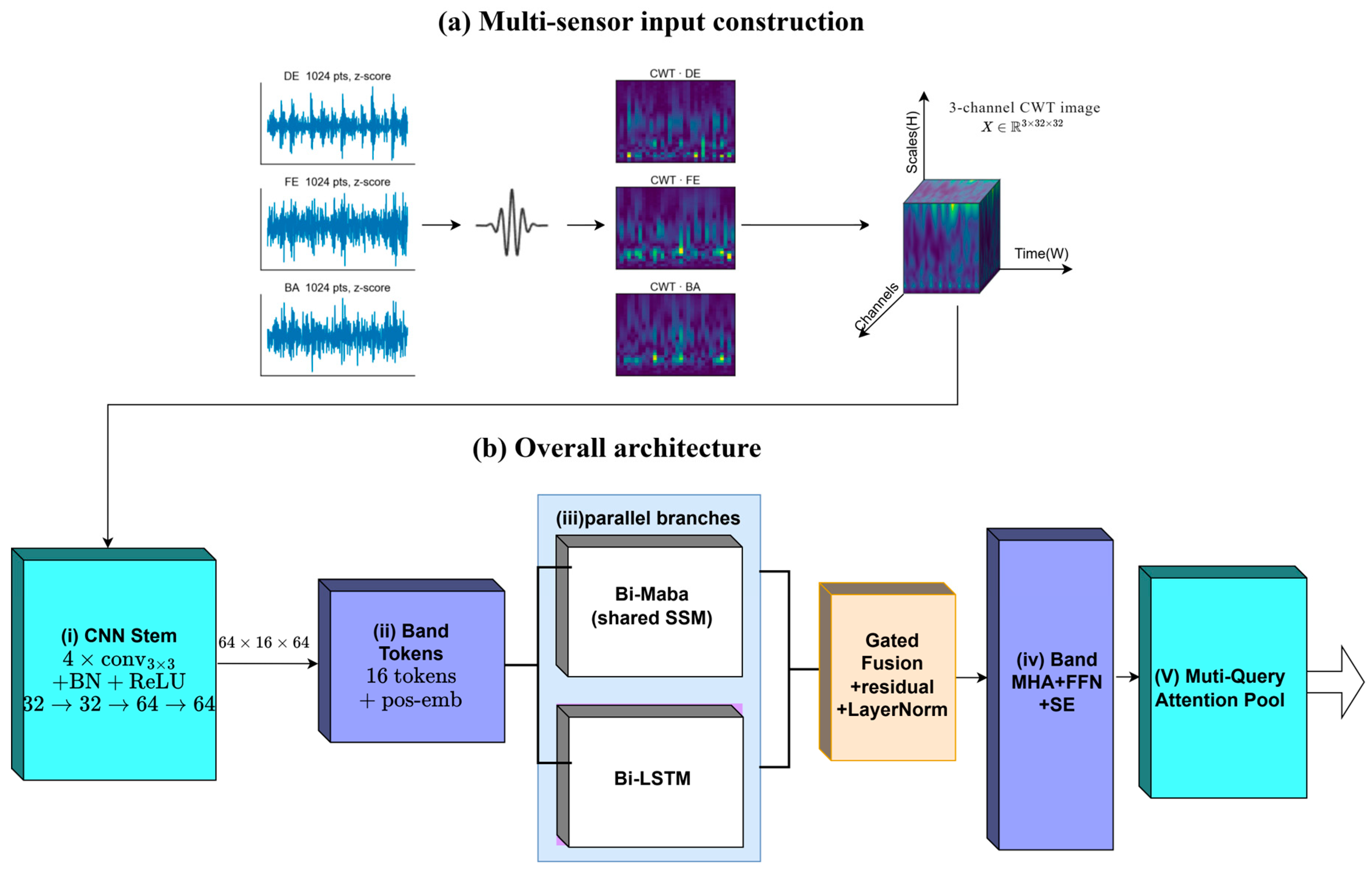
Figure 2.
Detailed structure of the gated bidirectional Mamba & BiLSTM frequency-band module (stage (iii) of Figure 1), including the shared bidirectional selective scan, the BiLSTM branch and the element-wise learned gate with residual connection.
Figure 2.
Detailed structure of the gated bidirectional Mamba & BiLSTM frequency-band module (stage (iii) of Figure 1), including the shared bidirectional selective scan, the BiLSTM branch and the element-wise learned gate with residual connection.
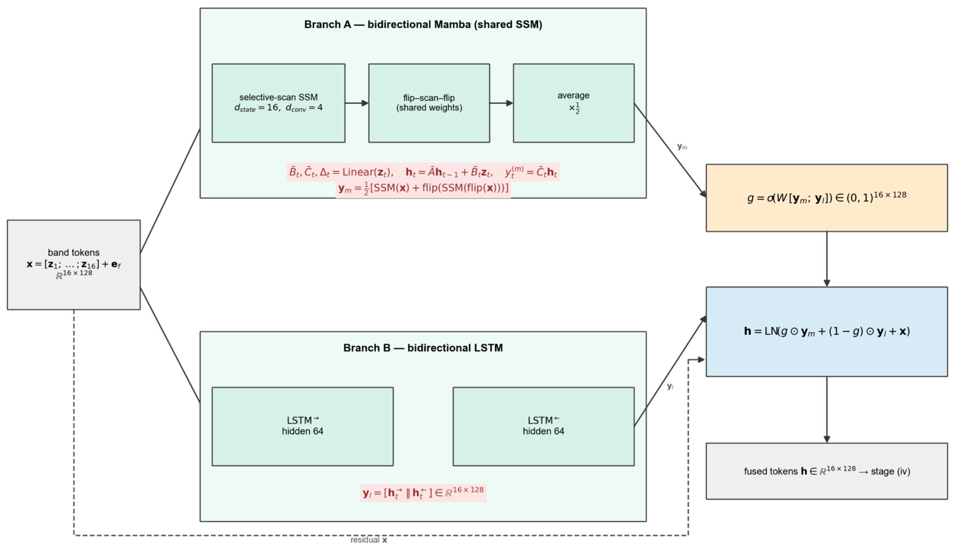
Figure 3.
Confusion matrix of MLBA-Net on the CWRU test set.
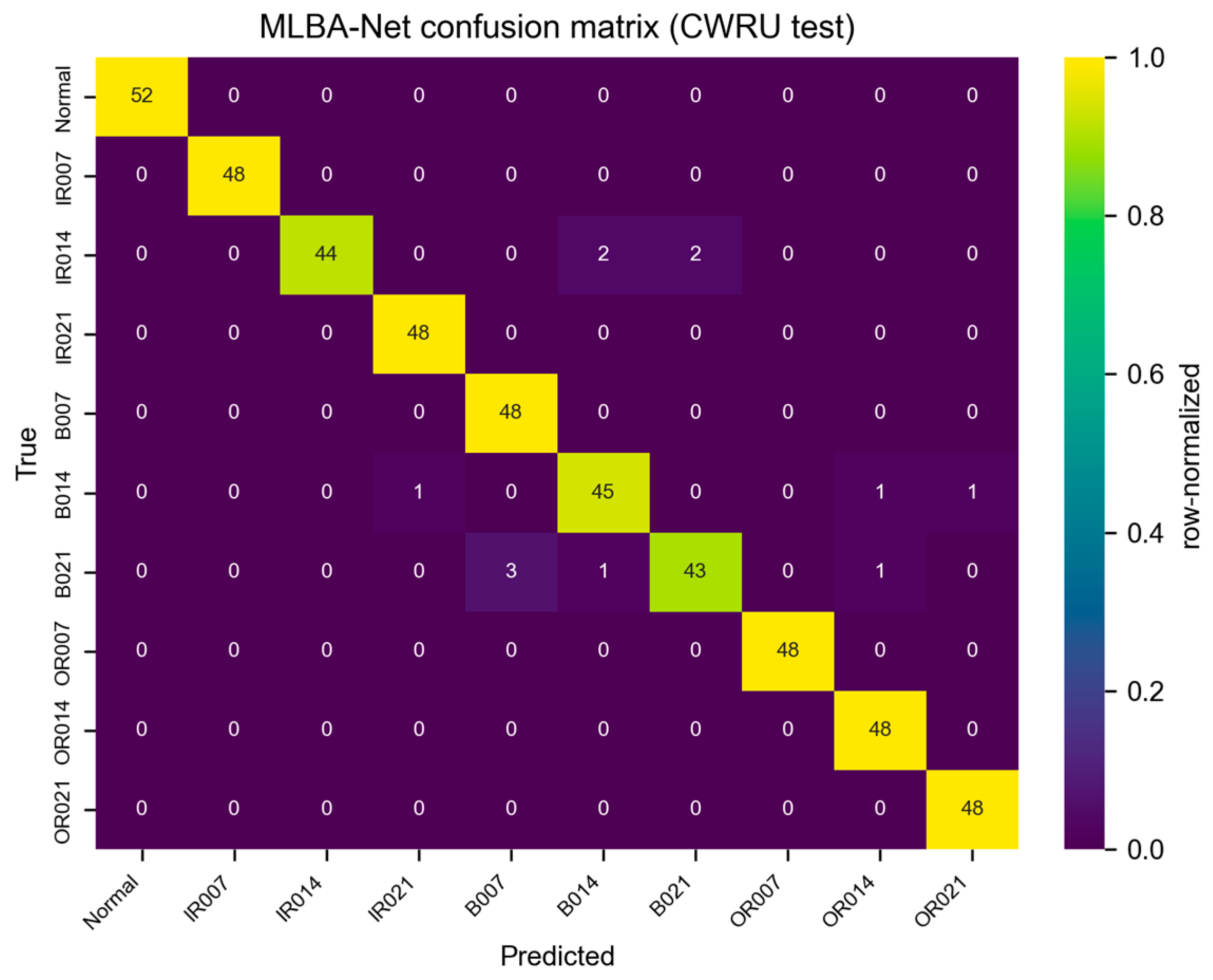
Figure 4.
Group-level confusion matrix of MLBA-Net in zero-shot CWRU→PU transfer.
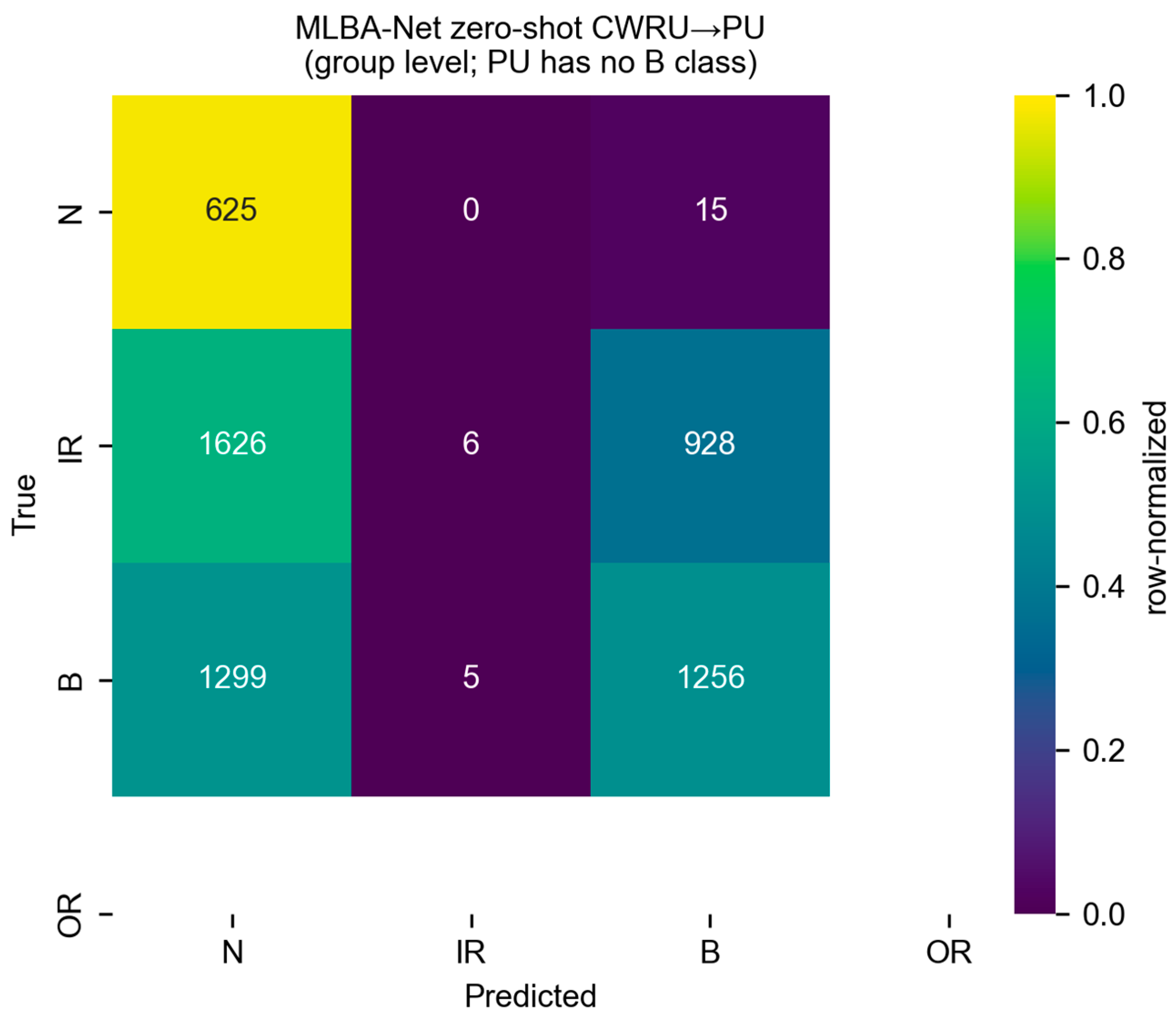
Figure 5.
Per-class zero-shot transfer accuracy heatmap on PU (mean over ten seeds; the group-level evidence of Table 4 is likewise ten-seed).
Figure 5.
Per-class zero-shot transfer accuracy heatmap on PU (mean over ten seeds; the group-level evidence of Table 4 is likewise ten-seed).
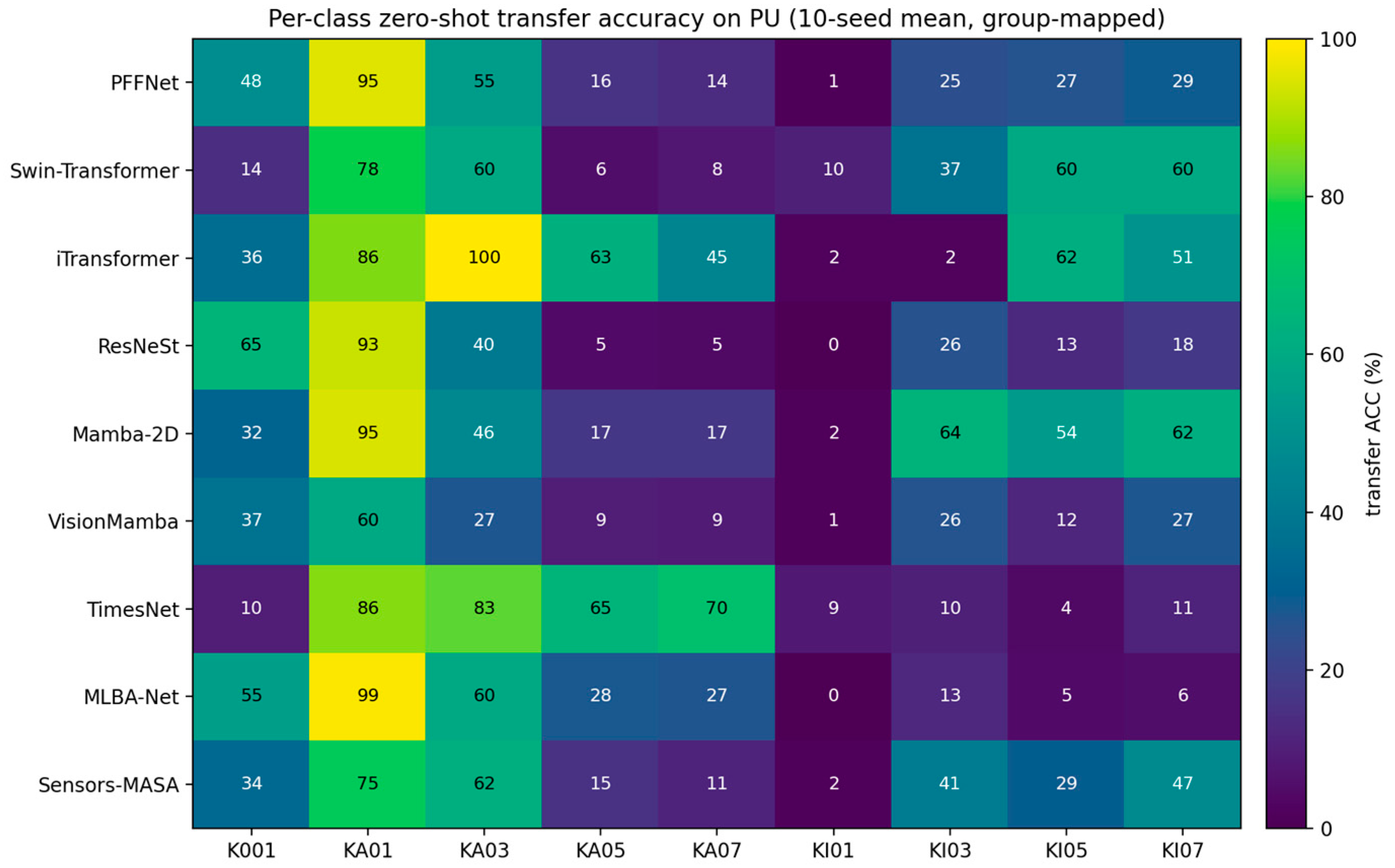
Figure 6.
Few-shot fine-tuning curves (group Macro-F1 vs. shots k, mean±SD, n=10): (a) CWRU→PU; (b) CWRU→SEU.
Figure 6.
Few-shot fine-tuning curves (group Macro-F1 vs. shots k, mean±SD, n=10): (a) CWRU→PU; (b) CWRU→SEU.
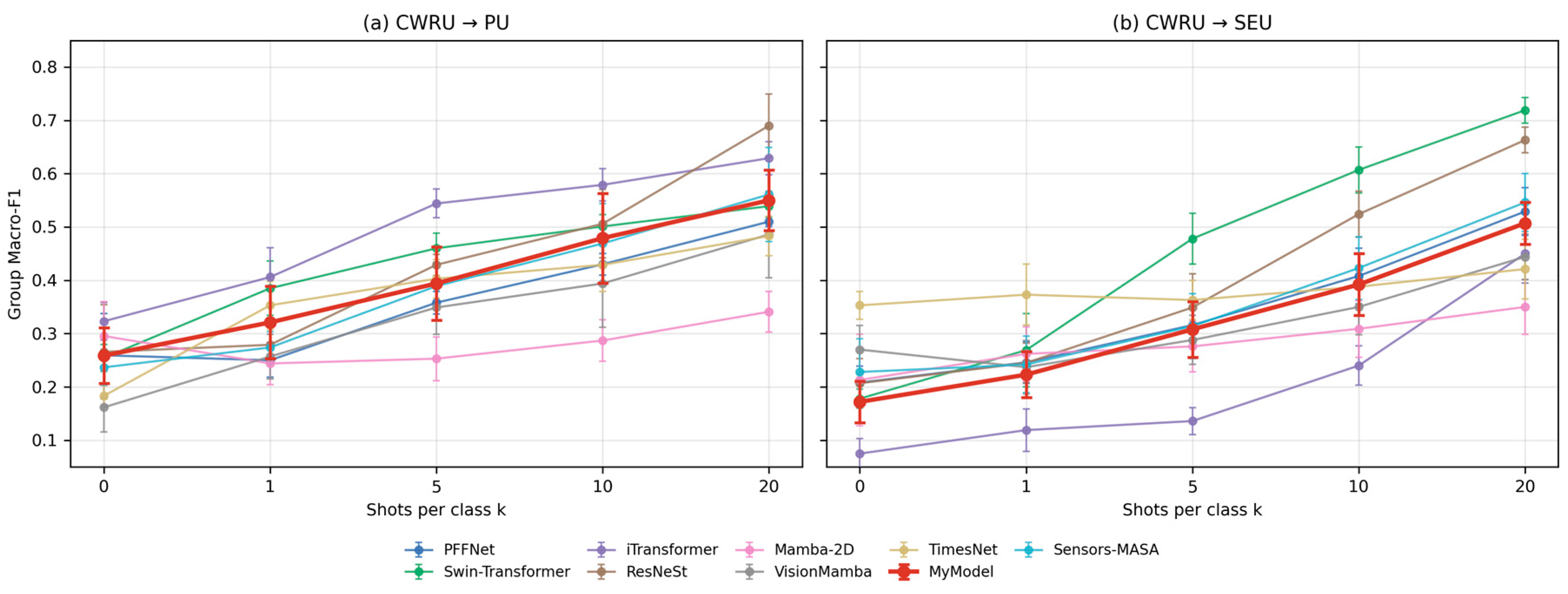
Figure 7.
Noise-robustness curves with noise-augmented training (n=10).
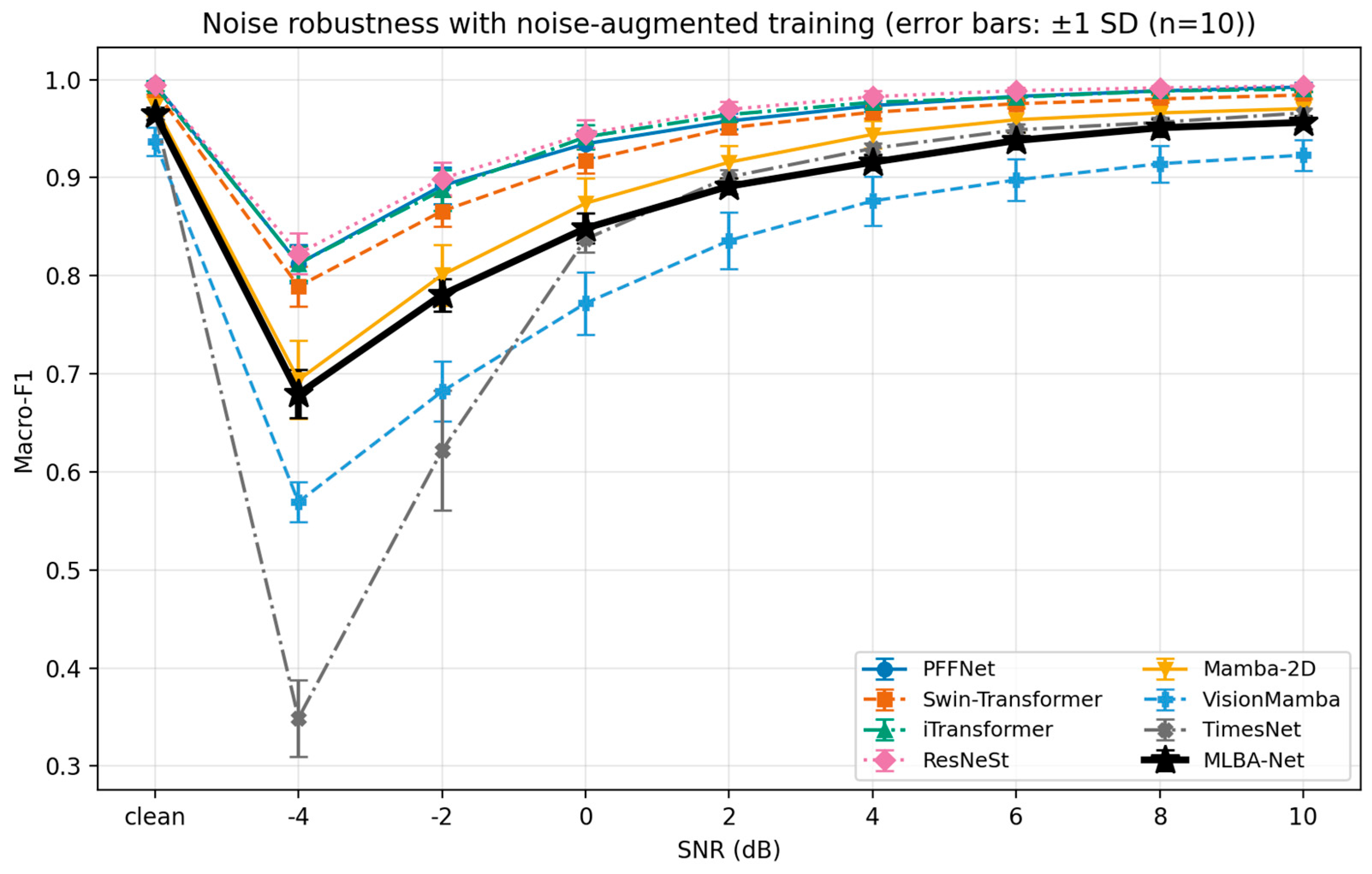
Figure 8.
Distribution of the fusion gate value g (Mamba-branch reliance) on CWRU (in-domain) and PU (cross-domain), n=10.
Figure 8.
Distribution of the fusion gate value g (Mamba-branch reliance) on CWRU (in-domain) and PU (cross-domain), n=10.
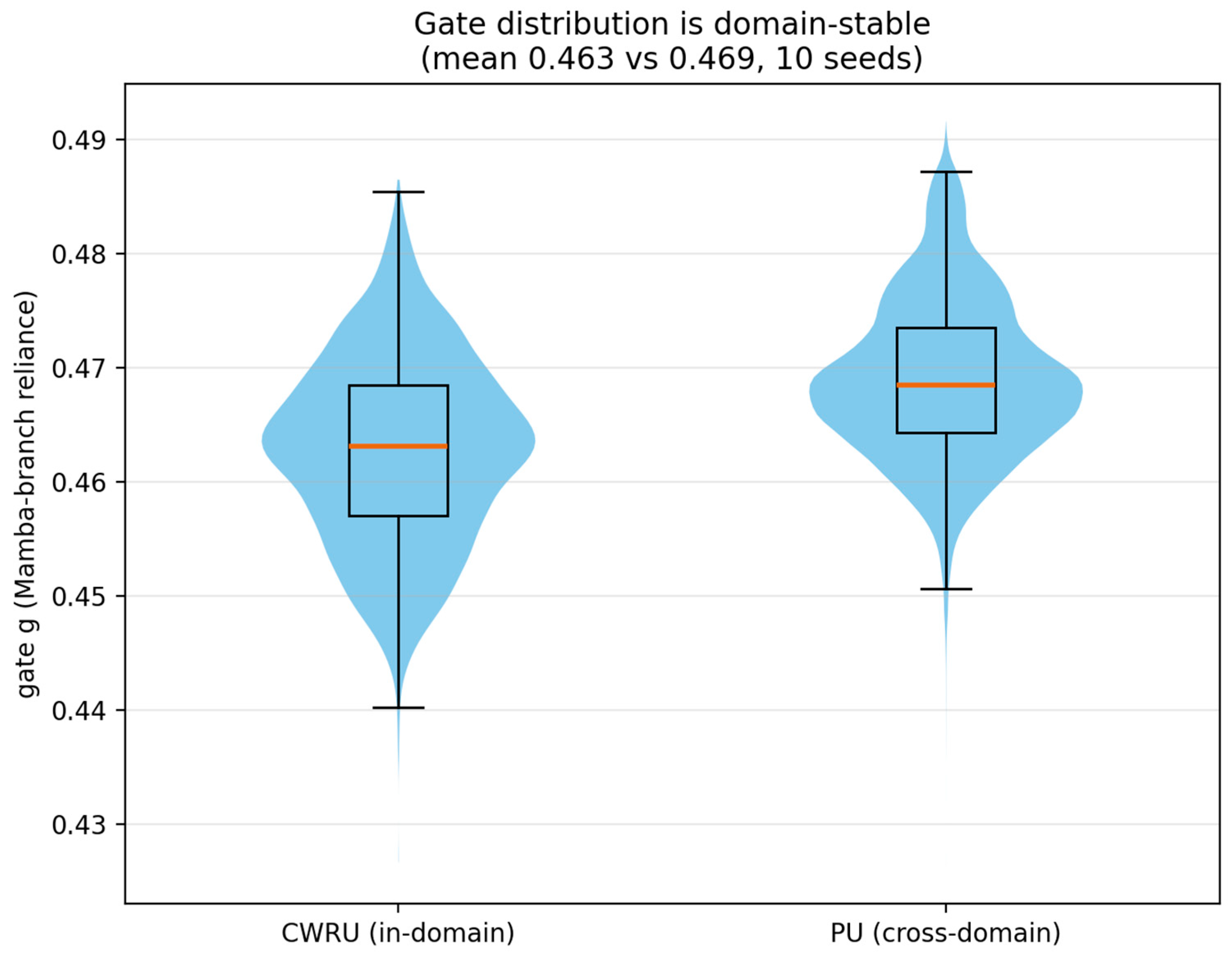
Figure 9.
Per-seed variance of in-domain Macro-F1 (left) and zero-shot transfer Macro-F1 (right) over ten seeds.
Figure 9.
Per-seed variance of in-domain Macro-F1 (left) and zero-shot transfer Macro-F1 (right) over ten seeds.
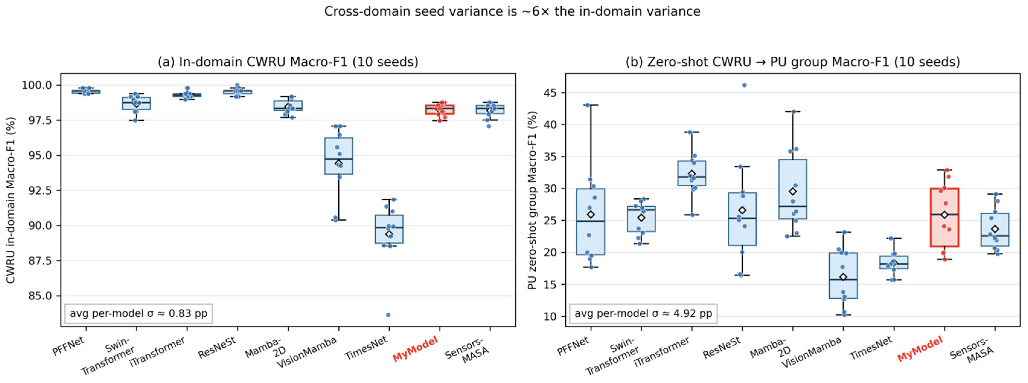
Figure 10.
Accuracy–efficiency landscape: parameters vs. in-domain accuracy (mean of 10 seeds).
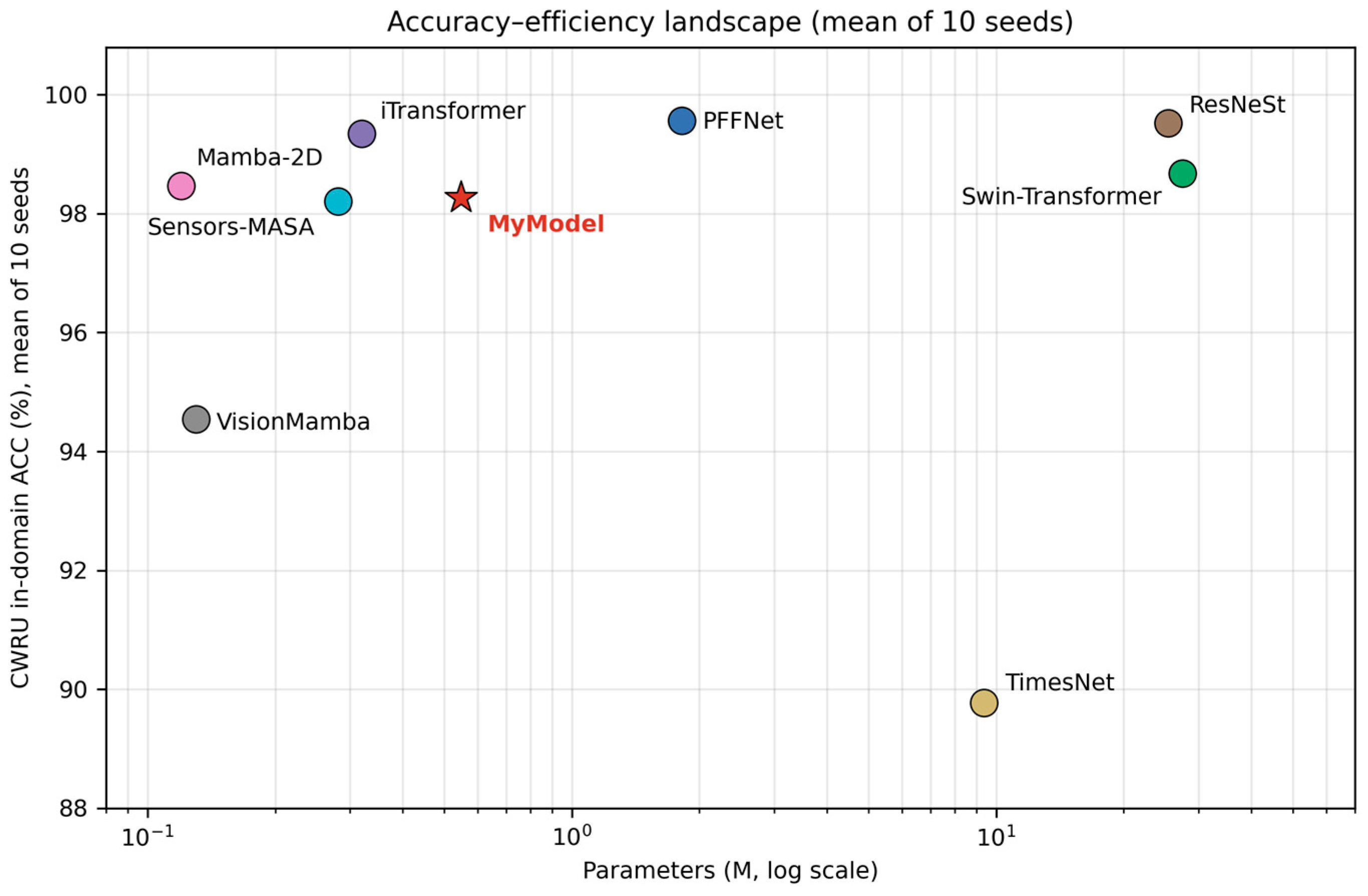
Table 1.
Positioning of representative studies on cross-domain and few-shot bearing fault diagnosis. Dashes indicate not reported or not applicable; readers are referred to the original papers for full details. The last column reports each study’s best published score on its primary task, with the metric annotated explicitly (acc. = accuracy; studies reporting only accuracy are quoted as such); the value for this work is the best cross-domain Macro-F1 (CWRU→PU, k=20).
Table 1.
Positioning of representative studies on cross-domain and few-shot bearing fault diagnosis. Dashes indicate not reported or not applicable; readers are referred to the original papers for full details. The last column reports each study’s best published score on its primary task, with the metric annotated explicitly (acc. = accuracy; studies reporting only accuracy are quoted as such); the value for this work is the best cross-domain Macro-F1 (CWRU→PU, k=20).
| Study | Datasets | Cross-domain | Few-shot | SSM-based | Noise eval. | Seeds | Best F1 / acc. |
| WDCNN [8] | CWRU et al. | DA design goal | No | No | Yes | Single | 100% (in-domain acc.) |
| DRSN [3] | CWRU | No | No | No | Yes | Single | 99.70% (clean, acc.) |
| DAN [14] / DANN [15] | Generic (non-bearing) | Yes (UDA) | No | No | No | – | – |
| MAML [17] / ProtoNet [18] | Generic (few-shot) | Task-level | Yes | No | No | – | – |
| Sensors 2025 [13] | CWRU, PU | Yes | Yes | Yes | Yes | – | 99.9% (0 dB, acc.) |
| This work | CWRU, PU, SEU | Yes (6 directions) | Yes (k=0–20) | Yes | Yes | 10 | 0.550 (k=20, Macro-F1) |
Table 2.
Module-level specification of MLBA-Net for a 3×32×32 input (d_model = 128). Parameter counts are exact counts of trainable tensors.
Table 2.
Module-level specification of MLBA-Net for a 3×32×32 input (d_model = 128). Parameter counts are exact counts of trainable tensors.
| Stage | Module | Configuration | Output tensor | Params |
| Stem | 4 × Conv2d 3×3 + BN + ReLU | channels 32→32→64→64; stride-2 on the 3rd layer only | B×64×16×16 | 65,760 |
| Tokenize | slice along F + Linear + band pos-emb | 16 bands; 1024→128; dropout 0.1 | B×16×128 | 133,248 |
| Branch A | shared Bi-Mamba (one MambaSSM) | d_state=16, d_conv=4; forward/backward weight-tied average | B×16×128 | 9,088 |
| Branch B | 1-layer BiLSTM | hidden 64 per direction (concat → 128) | B×16×128 | 99,328 |
| Fusion | element-wise gate + residual + LN | g=σ(W[y_m ; y_l]); residual is the token sequence Z | B×16×128 | 33,152 |
| Band attn | 1 × (MHA + FFN + SE) | 8 heads; FFN 128→256→128; SE reduction 4 | B×16×128 | 140,832 |
| Head | 4-query pool + MLP | concat 4×128; 512→128→10; no softmax | B×10 | 67,466 |
| Total | — | soft-threshold shrinkage disabled (Identity) | — | 548,874 |
Table 5.
Few-shot CWRU→PU fine-tuning: group Macro-F1 (mean±SD, n=10).
| Model | k=1 | k=5 | k=10 | k=20 |
| PFFNet | 0.250±0.032 | 0.358±0.021 | 0.430±0.020 | 0.510±0.009 |
| Swin-Transformer | 0.385±0.051 | 0.460±0.028 | 0.501±0.022 | 0.539±0.021 |
| iTransformer | 0.406±0.055 | 0.544±0.027 | 0.579±0.030 | 0.629±0.031 |
| ResNeSt | 0.279±0.033 | 0.429±0.020 | 0.506±0.064 | 0.690±0.059 |
| Mamba-2D | 0.244±0.040 | 0.253±0.041 | 0.287±0.039 | 0.341±0.038 |
| VisionMamba | 0.257±0.042 | 0.349±0.050 | 0.394±0.082 | 0.486±0.081 |
| TimesNet | 0.353±0.045 | 0.403±0.036 | 0.429±0.050 | 0.483±0.037 |
| Sensors-MASA | 0.274±0.030 | 0.389±0.045 | 0.469±0.075 | 0.561±0.088 |
| MLBA-Net (ours) | 0.321±0.068 | 0.394±0.069 | 0.479±0.084 | 0.550±0.057 |
Table 6.
Paired statistical comparisons of MLBA-Net against each baseline on CWRU→PU few-shot Macro-F1 (n=10 seeds; percentile bootstrap of the mean difference, 10,000 resamples; two-sided Wilcoxon signed-rank test). Positive Δ favors MLBA-Net.
Table 6.
Paired statistical comparisons of MLBA-Net against each baseline on CWRU→PU few-shot Macro-F1 (n=10 seeds; percentile bootstrap of the mean difference, 10,000 resamples; two-sided Wilcoxon signed-rank test). Positive Δ favors MLBA-Net.
| Comparison | k | ΔF1 | 95% bootstrap CI | p |
| vs. iTransformer | 1 | −0.085 | [−0.133, −0.038] | 0.014 |
| vs. Swin-Transformer | 1 | −0.064 | [−0.118, −0.001] | 0.084 |
| vs. TimesNet | 1 | −0.032 | [−0.074, +0.020] | 0.160 |
| vs. ResNeSt | 1 | +0.042 | [+0.008, +0.082] | 0.064 |
| vs. PFFNet | 1 | +0.071 | [+0.028, +0.119] | 0.020 |
| vs. Sensors-MASA | 1 | +0.048 | [+0.010, +0.091] | 0.065 |
| vs. VisionMamba | 1 | +0.064 | [+0.012, +0.131] | 0.027 |
| vs. Mamba-2D | 1 | +0.077 | [+0.034, +0.129] | 0.027 |
| vs. iTransformer | 5 | −0.150 | [−0.186, −0.108] | 0.002 |
| vs. Swin-Transformer | 5 | −0.066 | [−0.100, −0.024] | 0.010 |
| vs. Mamba-2D | 5 | +0.141 | [+0.095, +0.198] | 0.002 |
| vs. ResNeSt | 20 | −0.140 | [−0.184, −0.093] | 0.004 |
| vs. iTransformer | 20 | −0.080 | [−0.113, −0.049] | 0.002 |
| vs. TimesNet | 20 | +0.067 | [+0.016, +0.111] | 0.037 |
| vs. Mamba-2D | 20 | +0.208 | [+0.170, +0.246] | 0.002 |
Table 7.
In-domain results on SEU (5 classes, mean±SD, n=10 seeds).
| Model | ACC (%) | Macro-F1 | Macro-Recall (%) | Macro-AUC |
| PFFNet | 90.12±1.54 | 0.901±0.016 | 90.12±1.54 | 0.990±0.002 |
| Swin-Transformer | 93.08±1.10 | 0.931±0.011 | 93.08±1.10 | 0.994±0.001 |
| iTransformer | 95.42±0.64 | 0.954±0.006 | 95.42±0.64 | 0.997±0.001 |
| ResNeSt | 93.46±1.22 | 0.935±0.012 | 93.46±1.22 | 0.994±0.002 |
| Mamba-2D | 81.19±3.22 | 0.811±0.032 | 81.19±3.22 | 0.970±0.008 |
| VisionMamba | 74.65±4.39 | 0.746±0.045 | 74.65±4.39 | 0.933±0.019 |
| TimesNet | 82.31±1.51 | 0.823±0.015 | 82.31±1.51 | 0.968±0.004 |
| Sensors-MASA | 87.92±2.45 | 0.879±0.025 | 87.92±2.45 | 0.980±0.004 |
| MLBA-Net (ours) | 85.77±1.79 | 0.857±0.018 | 85.77±1.79 | 0.978±0.005 |
Table 8.
CWRU→SEU transfer at group level {N, IR, B, OR} (Macro-F1, mean±SD, n=10).
| Model | k=0 | k=1 | k=5 | k=10 | k=20 |
| PFFNet | 0.208±0.031 | 0.246±0.039 | 0.316±0.042 | 0.408±0.052 | 0.529±0.045 |
| Swin-Transformer | 0.178±0.018 | 0.269±0.069 | 0.478±0.048 | 0.607±0.043 | 0.719±0.024 |
| iTransformer | 0.075±0.028 | 0.119±0.040 | 0.136±0.025 | 0.240±0.037 | 0.450±0.055 |
| ResNeSt | 0.207±0.046 | 0.245±0.037 | 0.349±0.063 | 0.524±0.043 | 0.663±0.024 |
| Mamba-2D | 0.213±0.086 | 0.262±0.051 | 0.276±0.048 | 0.309±0.053 | 0.350±0.051 |
| VisionMamba | 0.270±0.045 | 0.237±0.050 | 0.288±0.046 | 0.350±0.052 | 0.444±0.043 |
| TimesNet | 0.353±0.026 | 0.373±0.057 | 0.363±0.037 | 0.388±0.039 | 0.421±0.056 |
| Sensors-MASA | 0.228±0.062 | 0.242±0.053 | 0.314±0.061 | 0.423±0.059 | 0.546±0.054 |
| MLBA-Net (ours) | 0.172±0.039 | 0.223±0.043 | 0.308±0.052 | 0.392±0.058 | 0.507±0.039 |
Table 9.
SEU cross-condition transfer (20_0 ⇄ 30_2; Macro-F1, mean±SD, n=10; five representative models).
Table 9.
SEU cross-condition transfer (20_0 ⇄ 30_2; Macro-F1, mean±SD, n=10; five representative models).
| Direction | Model | k=0 | k=1 | k=5 |
| 20_0→30_2 | PFFNet | 0.529±0.024 | 0.709±0.034 | 0.734±0.018 |
| 20_0→30_2 | iTransformer | 0.523±0.022 | 0.629±0.040 | 0.716±0.021 |
| 20_0→30_2 | ResNeSt | 0.540±0.021 | 0.725±0.030 | 0.790±0.036 |
| 20_0→30_2 | Mamba-2D | 0.565±0.021 | 0.615±0.035 | 0.651±0.027 |
| 20_0→30_2 | MLBA-Net (ours) | 0.511±0.031 | 0.618±0.030 | 0.662±0.030 |
| 30_2→20_0 | PFFNet | 0.580±0.013 | 0.584±0.051 | 0.627±0.033 |
| 30_2→20_0 | iTransformer | 0.582±0.016 | 0.578±0.034 | 0.597±0.021 |
| 30_2→20_0 | ResNeSt | 0.565±0.029 | 0.557±0.047 | 0.620±0.027 |
| 30_2→20_0 | Mamba-2D | 0.571±0.018 | 0.567±0.025 | 0.600±0.029 |
| 30_2→20_0 | MLBA-Net (ours) | 0.432±0.047 | 0.452±0.048 | 0.484±0.029 |
Table 10.
Reverse transfer from SEU (4-class source) to CWRU and PU (Macro-F1, mean±SD, n=10).
| Model | Target | k=0 | k=1 | k=5 | k=10 | k=20 |
| PFFNet | CWRU | 0.138±0.039 | 0.335±0.078 | 0.603±0.038 | 0.766±0.031 | 0.877±0.025 |
| Swin-Transformer | CWRU | 0.188±0.044 | 0.548±0.071 | 0.755±0.038 | 0.844±0.032 | 0.902±0.016 |
| iTransformer | CWRU | 0.170±0.023 | 0.297±0.025 | 0.450±0.042 | 0.655±0.065 | 0.808±0.025 |
| ResNeSt | CWRU | 0.090±0.018 | 0.396±0.069 | 0.661±0.041 | 0.834±0.022 | 0.916±0.014 |
| Mamba-2D | CWRU | 0.178±0.044 | 0.339±0.088 | 0.486±0.079 | 0.643±0.040 | 0.760±0.022 |
| VisionMamba | CWRU | 0.240±0.029 | 0.269±0.036 | 0.312±0.024 | 0.391±0.036 | 0.501±0.050 |
| TimesNet | CWRU | 0.253±0.062 | 0.298±0.093 | 0.376±0.111 | 0.528±0.102 | 0.695±0.041 |
| Sensors-MASA | CWRU | 0.210±0.048 | 0.335±0.047 | 0.524±0.067 | 0.690±0.056 | 0.827±0.028 |
| MLBA-Net (ours) | CWRU | 0.095±0.038 | 0.268±0.042 | 0.403±0.078 | 0.586±0.105 | 0.715±0.115 |
| PFFNet | PU | 0.097±0.041 | 0.226±0.044 | 0.318±0.039 | 0.395±0.038 | 0.461±0.023 |
| Swin-Transformer | PU | 0.157±0.020 | 0.284±0.054 | 0.357±0.025 | 0.416±0.061 | 0.449±0.020 |
| iTransformer | PU | 0.095±0.039 | 0.194±0.053 | 0.318±0.070 | 0.479±0.033 | 0.563±0.030 |
| ResNeSt | PU | 0.101±0.028 | 0.234±0.036 | 0.384±0.026 | 0.454±0.023 | 0.562±0.066 |
| Mamba-2D | PU | 0.183±0.045 | 0.185±0.054 | 0.256±0.061 | 0.325±0.051 | 0.418±0.064 |
| VisionMamba | PU | 0.106±0.037 | 0.212±0.028 | 0.259±0.020 | 0.283±0.025 | 0.317±0.029 |
| TimesNet | PU | 0.120±0.043 | 0.278±0.053 | 0.318±0.042 | 0.359±0.057 | 0.431±0.067 |
| Sensors-MASA | PU | 0.142±0.052 | 0.268±0.082 | 0.401±0.100 | 0.488±0.079 | 0.565±0.105 |
| MLBA-Net (ours) | PU | 0.110±0.029 | 0.240±0.029 | 0.338±0.052 | 0.418±0.064 | 0.521±0.048 |
Table 11.
Reverse transfer from PU (9-class source) to CWRU and SEU at group level {N, IR, OR} (Macro-F1, mean±SD, n=10).
Table 11.
Reverse transfer from PU (9-class source) to CWRU and SEU at group level {N, IR, OR} (Macro-F1, mean±SD, n=10).
| Model | Target | k=0 | k=1 | k=5 | k=10 | k=20 |
| PFFNet | CWRU | 0.256±0.037 | 0.346±0.047 | 0.613±0.089 | 0.754±0.083 | 0.912±0.028 |
| Swin-Transformer | CWRU | 0.297±0.040 | 0.605±0.068 | 0.865±0.036 | 0.937±0.012 | 0.969±0.009 |
| iTransformer | CWRU | 0.256±0.084 | 0.436±0.080 | 0.655±0.062 | 0.797±0.047 | 0.896±0.019 |
| ResNeSt | CWRU | 0.265±0.093 | 0.390±0.072 | 0.784±0.053 | 0.928±0.019 | 0.973±0.004 |
| Mamba-2D | CWRU | 0.249±0.088 | 0.336±0.073 | 0.429±0.083 | 0.605±0.070 | 0.798±0.037 |
| VisionMamba | CWRU | 0.256±0.064 | 0.339±0.063 | 0.482±0.087 | 0.625±0.088 | 0.760±0.062 |
| TimesNet | CWRU | 0.149±0.024 | 0.476±0.114 | 0.723±0.057 | 0.813±0.048 | 0.889±0.035 |
| Sensors-MASA | CWRU | 0.277±0.086 | 0.477±0.120 | 0.764±0.081 | 0.914±0.033 | 0.959±0.012 |
| MLBA-Net (ours) | CWRU | 0.307±0.092 | 0.430±0.100 | 0.623±0.095 | 0.791±0.064 | 0.898±0.037 |
| PFFNet | SEU | 0.211±0.043 | 0.298±0.072 | 0.358±0.051 | 0.466±0.041 | 0.564±0.034 |
| Swin-Transformer | SEU | 0.193±0.031 | 0.347±0.047 | 0.450±0.049 | 0.555±0.061 | 0.672±0.055 |
| iTransformer | SEU | 0.182±0.049 | 0.237±0.073 | 0.258±0.069 | 0.406±0.075 | 0.593±0.061 |
| ResNeSt | SEU | 0.218±0.051 | 0.286±0.076 | 0.441±0.055 | 0.590±0.052 | 0.720±0.029 |
| Mamba-2D | SEU | 0.192±0.037 | 0.246±0.034 | 0.286±0.064 | 0.355±0.058 | 0.473±0.050 |
| VisionMamba | SEU | 0.222±0.034 | 0.269±0.051 | 0.316±0.045 | 0.433±0.043 | 0.522±0.041 |
| TimesNet | SEU | 0.195±0.026 | 0.394±0.044 | 0.446±0.032 | 0.490±0.034 | 0.575±0.038 |
| Sensors-MASA | SEU | 0.239±0.065 | 0.332±0.071 | 0.448±0.059 | 0.554±0.074 | 0.639±0.065 |
| MLBA-Net (ours) | SEU | 0.253±0.060 | 0.299±0.047 | 0.384±0.076 | 0.470±0.069 | 0.573±0.039 |
Table 12.
Sensor-configuration isolation (Macro-F1, mean±SD, n=10). Source: multi = genuine multi-sensor input; rep = single channel replicated ×3. Targets: PU (replicated), SEU-multi (genuine), SEU-rep (replicated). All cells are evaluated on the 1,440-segment evaluation pool that is strictly disjoint from the support pool (the same pool as in the few-shot protocol of Section 3.10), so that the k=0 and k≥1 columns share one evaluation protocol; the k=0 column therefore differs slightly from the zero-shot results of Table 4, which use the full 5,760-segment PU test set (differences ≤0.014, well within seed noise).
Table 12.
Sensor-configuration isolation (Macro-F1, mean±SD, n=10). Source: multi = genuine multi-sensor input; rep = single channel replicated ×3. Targets: PU (replicated), SEU-multi (genuine), SEU-rep (replicated). All cells are evaluated on the 1,440-segment evaluation pool that is strictly disjoint from the support pool (the same pool as in the few-shot protocol of Section 3.10), so that the k=0 and k≥1 columns share one evaluation protocol; the k=0 column therefore differs slightly from the zero-shot results of Table 4, which use the full 5,760-segment PU test set (differences ≤0.014, well within seed noise).
| Model | Source | PU k=0 | PU k=1 | PU k=5 | SEU-m k=0 | SEU-m k=5 | SEU-r k=0 | SEU-r k=5 |
| PFFNet | multi (DE/FE/BA) | 0.273±0.073 | 0.250±0.032 | 0.358±0.021 | 0.208±0.031 | 0.317±0.042 | 0.111±0.013 | 0.375±0.032 |
| PFFNet | rep (DE×3) | 0.265±0.007 | 0.280±0.024 | 0.358±0.019 | 0.141±0.044 | 0.368±0.047 | 0.148±0.055 | 0.387±0.030 |
| iTransformer | multi (DE/FE/BA) | 0.336±0.046 | 0.406±0.055 | 0.544±0.027 | 0.075±0.028 | 0.136±0.025 | 0.172±0.068 | 0.137±0.021 |
| iTransformer | rep (DE×3) | 0.246±0.018 | 0.319±0.024 | 0.474±0.070 | 0.108±0.008 | 0.119±0.030 | 0.200±0.023 | 0.115±0.018 |
| ResNeSt | multi (DE/FE/BA) | 0.274±0.083 | 0.279±0.033 | 0.429±0.020 | 0.207±0.046 | 0.350±0.062 | 0.117±0.015 | 0.381±0.046 |
| ResNeSt | rep (DE×3) | 0.251±0.005 | 0.255±0.024 | 0.407±0.032 | 0.187±0.079 | 0.421±0.040 | 0.105±0.005 | 0.433±0.036 |
| Mamba-2D | multi (DE/FE/BA) | 0.297±0.062 | 0.244±0.040 | 0.253±0.041 | 0.213±0.086 | 0.276±0.048 | 0.200±0.056 | 0.300±0.061 |
| Mamba-2D | rep (DE×3) | 0.230±0.020 | 0.243±0.032 | 0.261±0.041 | 0.230±0.068 | 0.279±0.066 | 0.231±0.093 | 0.345±0.050 |
| MLBA-Net (ours) | multi (DE/FE/BA) | 0.261±0.052 | 0.321±0.068 | 0.394±0.069 | 0.172±0.039 | 0.308±0.052 | 0.133±0.023 | 0.298±0.072 |
| MLBA-Net (ours) | rep (DE×3) | 0.247±0.025 | 0.264±0.034 | 0.319±0.059 | 0.151±0.032 | 0.281±0.060 | 0.082±0.020 | 0.174±0.033 |
Table 13.
Noise robustness with noise-augmented training for all models (Macro-F1 on CWRU test, mean±SD, n=10).
Table 13.
Noise robustness with noise-augmented training for all models (Macro-F1 on CWRU test, mean±SD, n=10).
| Model | clean | −4 dB | 0 dB | 10 dB |
| PFFNet | 0.995±0.002 | 0.812±0.019 | 0.935±0.014 | 0.992±0.005 |
| Swin-Transformer | 0.989±0.004 | 0.789±0.020 | 0.917±0.012 | 0.984±0.003 |
| iTransformer | 0.994±0.005 | 0.813±0.017 | 0.942±0.012 | 0.990±0.003 |
| ResNeSt | 0.995±0.002 | 0.823±0.021 | 0.945±0.014 | 0.994±0.003 |
| Mamba-2D | 0.973±0.010 | 0.694±0.040 | 0.874±0.025 | 0.970±0.010 |
| VisionMamba | 0.937±0.014 | 0.569±0.020 | 0.772±0.032 | 0.923±0.016 |
| TimesNet | 0.966±0.006 | 0.349±0.039 | 0.837±0.014 | 0.966±0.005 |
| MLBA-Net (ours) | 0.965±0.006 | 0.679±0.025 | 0.848±0.015 | 0.956±0.007 |
Table 14.
Multi-seed architecture ablation of MLBA-Net (mean±SD, n=10 seeds).
| Variant | Params (M) | CWRU ACC (%) | CWRU F1 (%) | PU 1-shot F1 | PU 5-shot F1 |
| base: BiMamba ∥ BiLSTM, learnable gate | 0.549 | 98.26±0.43 | 98.25±0.44 | 0.321±0.068 | 0.394±0.069 |
| Mamba only (no LSTM branch) | 0.417 | 98.18±0.69 | 98.17±0.69 | 0.344±0.042 | 0.434±0.061 |
| LSTM only (no Mamba branch) | 0.507 | 98.57±0.33 | 98.56±0.33 | 0.316±0.031 | 0.403±0.062 |
| No gate (branch sum) | 0.516 | 98.20±0.48 | 98.19±0.48 | 0.334±0.032 | 0.448±0.077 |
| Fixed gate g=0.5 | 0.516 | 98.20±0.65 | 98.19±0.65 | 0.321±0.029 | 0.450±0.080 |
| Fixed gate g=0.3 (LSTM-leaning) | 0.516 | 98.18±0.62 | 98.16±0.63 | 0.319±0.031 | 0.443±0.086 |
| BiGRU replaces Mamba | 0.603 | 98.31±0.58 | 98.29±0.59 | 0.315±0.032 | 0.456±0.068 |
| No band attention | 0.483 | 97.93±0.51 | 97.91±0.51 | 0.293±0.042 | 0.373±0.035 |
| No SE re-weighting | 0.541 | 98.29±0.39 | 98.27±0.40 | 0.333±0.034 | 0.429±0.084 |
| Average pooling (replaces multi-query) | 0.499 | 98.33±0.61 | 98.32±0.61 | 0.322±0.025 | 0.446±0.083 |
| Patch tokens (replace band tokens) | 0.457 | 98.60±0.69 | 98.59±0.70 | 0.325±0.053 | 0.449±0.069 |
Disclaimer/Publisher’s Note: The statements, opinions and data contained in all publications are solely those of the individual author(s) and contributor(s) and not of MDPI and/or the editor(s). MDPI and/or the editor(s) disclaim responsibility for any injury to people or property resulting from any ideas, methods, instructions or products referred to in the content. |
© 2026 by the authors. Licensee MDPI, Basel, Switzerland. This article is an open access article distributed under the terms and conditions of the Creative Commons Attribution (CC BY) license (http://creativecommons.org/licenses/by/4.0/).
Copyright: This open access article is published under a Creative Commons CC BY 4.0 license, which permit the free download, distribution, and reuse, provided that the author and preprint are cited in any reuse.