
Submitted:
24 September 2026
Posted:
28 September 2026
You are already at the latest version
Abstract
A two-field configuration cannot generally be reduced to a single scalar while preserving its dynamics, because discarding its internal relative structure omits positive internal stress and thereby artificially lowers the stress represented in the reduced description. In a specified two-field model, three gradient and two contact channels fix the compression generator \(2I_3\oplus3I_2\) and internal virial \(2E_s+3E_a\). The resulting energy carrier yields a sharp entropy-virial bound, attained by smooth fields and strengthened at fixed positive core density. Restricted weak-field GR profile tests use 153 SPARC galaxies, withholding 659 outer observations in 131. With matched stellar, distance and inclination priors, the fixed-shape core lowers median outer loss from 24.46 for the adopted baryonic source to 3.89: an 84.1% reduction (paired-bootstrap 95% interval 75.9-90.8%). It wins 101/131 comparisons, or 100/130 excluding one infeasible baseline. Under independent galaxy signs and equal win probabilities, the five-test Holm-adjusted \(p=7.00\times10^-10\) has two-sided Gaussian equivalent \(Z=6.17\). Navarro-Frenk-White retains lower median outer loss, 1.97, and wins 87/131 comparisons against the core (\(Z=3.52\), separate three-test correction). All comparisons use the same GR law. The fitted cores have zero excess internal stress; these retrospective tests do not uniquely identify entropy geometry. Common baryonic gravity preserves the model's unexcited mixed sector; internal stress supports the field, while tracers respond to gravity. Physical validation requires shared-parameter equilibria in the combined baryonic and field potential, calibrated uncertainties and independent evaluation.
Keywords:
directional shear
; quantum relative entropy
; virial theorem
; multicomponent fields
; dark sectors
1. Introduction
Internal field energies can supply stress omitted by a scalar density-current closure. We relate their compression response to channel entropy, mechanical support and gravity, retaining both energy partition and intensity.
Section 2 and Supplemental Material S1 construct the oscillator family and two-moment entropy projection, following the input discipline of Refs. [1,2]. Field promotion, conservative energy and Einstein gravity are constitutive premises. Nonrelativistic matching [4,5] and spinor hydrodynamics [6,7] supply the frameworks; the model-specific coefficients and domain arguments are derived here.
Three gradient channels and an irredundant two-square contact completion give positive energy blocks with traces . Fixed-number compression fixes their weights, the generator and virial . The finite-population kurtosis bound [3] makes its centered direction a minimum of normalized tracial shear, with the balanced grading of controlled completion [1]. This spectral compatibility presupposes the field and channel convention; it selects neither interactions nor a physical gauge action.
The field-specific contributions are the feature lift fixing the generator’s scale and scalar part, smooth-field attainment of the entropy-virial bound at prescribed number and energy, its strengthening at fixed positive core density, and different channel entropies at identical mechanical data. Exponential tilting and the free-energy identity [10,11] supply the statistical framework. The thermal result calibrates work for a controlled register. S15 separates cubic susceptibility from field evolution; S13.8-S13.10 state the additional assumptions needed for an outer population. The mechanical analysis establishes a stable mixed minimizing set and gapped internal modes with no first-order Poisson-source perturbation. Omitted stress can generate circulation and density redistribution.
Section 2, Section 3, Section 4 and Section 5 establish the field model and stress; Section 6 and Section 7 develop the channel geometry and thermodynamics. Section 8 derives gravitational response, followed by observational tests and controlled calculations in Section 9. The supplement supplies proofs and reproducible methods.
2. Preparation Statistics and Field Model
2.1. Preparation Family and Information Retained
On let r be multiplication, , and define the positive oscillator by the closed form
For and , its faithful Gibbs family is
Here and are raw moments. The unitary dilation preserves the form domain and satisfies . Its Hermite spectrum gives the geometric Gibbs weights, partition function and finite entropy in (2.1); dilation gives the two moments. Section S1 supplies these steps and the finite-moment extension.
For the finite contrast and its coincidence Hessian are
The finite expectation and Gibbs logarithm give the contrast. Its derivatives give the positive Bogoliubov-Kubo-Mori (BKM) metric without differentiating an unbounded trace.
The two-moment maximum-entropy closure has the explicit form
For a microscopic state with these finite moments and any preparation reference ,
Finite oscillator energy bounds entropy; moment matching gives (2.5) and unique entropy maximization (S1). This raw-moment closure can discard means, cross correlations and non-Gaussianity [8,9]. The nonlinear projection is not a quantum channel.
2.2. Retained and Discarded Preparation Free Energy
Corollary 2.1
(Free-energy budget of the preparation projection). Fix and a reference , and set
For a density operator ϱ with finite raw moments , , and its projection from (2.4),
Both relative-entropy terms are nonnegative. The discarded term vanishes precisely when .
Proof.
All terms are finite by the preceding moment bound. The Gibbs logarithm gives ; combine this with (2.5). Moment matching preserves , proving the second identity. □
This fixed-Hamiltonian gap establishes neither relaxation nor field polarization energy. Converting it to potential density requires a density or volume calibration.
In expectation coordinates , (Section S1.2). In a nonlinear chart the ordinary Hessian can differ from the metric away from the reference: at ,
At the reference, the ordinary and covariant Hessians of the contrast equal because its gradient vanishes.
2.3. Constitutive Assumptions and Field Action
Fix , put , and define
Both and vanish only at the reference and have Hessian there. Corollary 2.1 identifies as a normalized fixed-Hamiltonian free-energy gap. The matter results use the constitutive choice .
Constitutive premise A1
(Retained state variables). The faithful two-moment labels of one canonical bosonic mode are promoted to two local classical scalar fields. The microscopic carrier and the physical sufficiency of these retained variables are not derived.
Constitutive premise A2
(Comparison energy). A fixed reference and the full choice or determine . The leading isotropic spatial stiffness is the coincidence-Hessian tensor of the two-point contrast, with a common positive calibration .
Constitutive premise A3
(Minimal Lorentzian completion). At retained order the scalar action is local, Lorentz invariant and quadratic in first derivatives, with no preferred spacetime tensor besides the metric. Gravity is Einstein-Hilbert; other retained matter is separately minimally coupled. Nonminimal curvature and additional derivative operators are excluded at this order.
Lorentz invariance in this derivative class gives the coefficient ; matching arbitrary static gradients fixes . Set and . The action is
This sigma-model completion ([12], Section 2) has common reference mass
The constants , reference and offset remain inputs. Adding preserves the reference metric but changes higher interactions; changing inertia or adding a quadratic deformation can split the masses. No radiative protection is implied.
3. Matched Interaction and Mixed Matter Phase
3.1. One Ratio Fixes the Normalized Contact Pattern
Assume , , weak gravity and interaction frequency shifts much smaller than m. Tree-level nonrelativistic matching retains rest-frequency derivative terms [4,5]. We match short-range interactions in the local gravity-decoupled flat-space limit, excluding the gravitational pole [13], then restore gravity through Poisson’s equation.
Let and set
Here is an interaction ratio, not a radius. For canonical envelopes , the matched contact energy is
with
Section S2 derives the model-specific fourth jet and derivative vertex; Ref. [14] gives the general geometric framework. Pair conversion survives equal-frequency averaging: total number, but not component numbers, is conserved exactly in the leading equations and approximately in the real-field theory.
The contacts obey
This restricts the full comparison potential beyond its masses and reference metric. For , the deformation preserves those quadratic data and the kinetic metric, but shifts the leading contacts in the same canonical frame by
These shifts distinguish comparison energies in the specified canonical frame (S2). Inferring and requires preparation and readout of those channels; equal free masses do not identify them. Otherwise the physical test requires the full contact tensor modulo admissible basis changes. The null relation is necessary but insufficient in this frame, and density or circular-speed data measure neither contact.
3.2. Internal Minimum and Pressure Branch
Define
For either sign let .
Theorem 3.1
(Mixed sector and unique repulsive branch). At fixed total density n, the contact is minimized by and relative phase . Its value is . The embedding
is invariant under the leading field equations with a common Newtonian potential. Moreover
Proof.
Since , phase minimization gives . Put and . The remaining contact shape is exactly
Both component chemical forces at the minimum equal , so the common kinetic and gravitational operators preserve (3.7). The function has positive derivative and vanishes at zero. Consequently decreases strictly from one to zero. The factorization of proves the unique transition; gives the composition interval. The stated decimal value supplements, rather than proves, uniqueness. □
A single-component condensate does not minimize internal energy: rotating to preserves density and gradient energy but changes the energy by
The coefficient has the sign of , so single-component repulsion does not ensure internal stability. For , concentration makes the quartic truncation unbounded below, without establishing the behavior of the exact high-density action.
The invariant mixed sector requires equal retained component frequencies. At fixed contacts and common kinetic and gravitational coefficients, shifts the local minimizing fraction away from the original mixed line. S2 gives the density-dependent local thresholds. This pointwise diagnostic does not solve spatial equilibrium: a detuned profile requires the coupled equations with gradient energy. No radiative splitting magnitude is inferred.
4. Energy, Stability and the Internal Spectrum
Consider the isolated, nonexpanding leading theory on , with , and no component-number or angular-momentum constraints. Write
Rest energy is omitted. Its Hamiltonian flow is
Hereafter unmarked spatial integrals are over and Sobolev norms use fixed units.
Let be (4.1) with a real scalar amplitude u and contact . For the exact defect is
Contact square completion and the vector diamagnetic inequality give nonnegativity; gravity cancels at fixed density. The mixed embedding attains the scalar energy, so both fixed-N infima equal .
Theorem 4.1
(Leading ground states and nonlinear stability). For every the fixed-number infimum is attained, and at least one amplitude is positive, radial decreasing, regular and exponentially decaying. Its mixed lift is stationary. For every datum, Eq. (4.2) has a unique global solution in , with two complex components, conserving energy and number, with
The complete fixed-N minimizing set , including translations, common phases and both mixed branches, is orbitally stable: for every there is such that
The nearby datum need not have exactly number N; its own number is conserved.
S3 proves scalar existence by coefficient rescaling ([15], Theorem 2.7), global flow by finite-component Cauchy estimates and coercivity, and orbital stability by strict binding and compactness of vector minimizing sequences [16,17,18].
Every minimizer has a positive scalar amplitude and constant minimizing orientation. Scalar variation and equality in (4.3) give
Writing for the mixed-branch contact energy, the stationary virial identities ([19], Section III.2) give and . Stability of the minimizing set establishes neither uniqueness, attraction, formation nor membership of a numerical branch. Leading-theory control does not guarantee microscopic dilution or relativistic regularity.
4.1. The Scalar Spectral Gap of a Fixed Core
Lemma 4.2
(Frozen-core gap and weighted variance). Let be a smooth exponentially decaying stationary scalar core from (4.6), with , and . Let be its isolated Newtonian potential. On define
This self-adjoint operator has domain , form domain , and
For real f with in the ground-state form domain, writing , one has
Proof.
The ground-state transform gives , proving positivity and the simple kernel by form closure. The bounded decaying potential gives ([20], Theorems 6.19 and 10.2), so zero is isolated. Apply the gap to to obtain (4.9). Supplemental Material, Section S10.2, proves the domain and compactness steps. □
This frozen-potential gap differs from the coupled density Hessian and leaves the full theory’s phase and translation symmetries intact.
4.2. A Global Internal Gap and Infinitely Many Bound Modes
Positive anisotropy opens an internal gap despite the vanishing density at infinity; the Newtonian tail binds infinitely many modes below the continuum.
Theorem 4.3
(Gapped internal spectrum of a positive mixed core). Let be a mixed stationary state of the repulsive leading theory, with smooth and exponentially decaying, , and . In particular, a positive radial minimizing state supplied by Theorem 4.1 satisfies these conditions. Fix with the same branch sign as c, and write the internal perturbation as with real . Define
The exact first-order internal system and its conserved quadratic energy are
The operators are self-adjoint on , with form domain , and
The energy is equivalent to , so the linear internal evolution is bounded for all time in . Its squared-frequency operator is the positive self-adjoint operator associated with the closed form
It satisfies
where are infinitely many discrete eigenvalues, counted with multiplicity. The lowest frequency also obeys
Every such internal mode has identically zero first-order density, number-current and Poisson-source perturbations.
Proof.
The contact expansion in the frame gives (4.13) (Supplemental Material, Section S2). Lemma 4.2 and exclude zero eigenvectors of ; their essential spectra start at , so both are strictly positive. Their forms are equivalent to the norm and conserve . The substitution gives .
With , compactness of the decaying potentials implies that is compact, fixing the continuum threshold. For , Cauchy-Schwarz gives
The tail dominates the kinetic energy on large disjoint annuli. Their finite spans have both Rayleigh quotients below ; min-max therefore gives arbitrarily many eigenvalues below . Taking proves the frequency bound. Finally, makes density and current first variations vanish, and hence the isolated Poisson variation vanishes. Supplemental Material, Section S10.1, supplies the closed-form operator construction and annular estimates. □
The bound uses the number-weighted density ; the gap need not be uniform in N or as . Linear stability permits second-order sourcing and establishes neither damping, equilibration nor nonlinear persistence. Positive anisotropy and a Newtonian tail support this mechanism beyond the matched coefficients.
5. Internal Stress and Scalar Closure
5.1. Polarization Is the Missing Component Variable
On a smooth positive-density region define the unit polarization and number velocity by
Polarization describes the components, not microscopic dark-matter spin. The energies decompose as
Contact square completion gives the first identity; the spinor gradient decomposition [6,7] gives the second (normalization in Section S4.1).
The projective metric [21] governs envelope orientation, while the preparation BKM metric fixes anisotropy. Locally,
This texture-vorticity relation [22] introduces no independent gauge field. At nodes we use the stress formulation below.
Let , , and introduce
The complex-field momentum balance for this quartic contact is
Section S4.2 derives the identity and its energy-space interpretation from (4.2).
5.2. An Energy Bound on the Omitted Equation Term
Scalar closure retains the mixed pressure and scalar gradient stress at the actual ; vortical data need not admit a scalar wavefunction.
Theorem 5.1
(Positive closure stress and its energy budget). For a nonzero configuration of the repulsive leading theory, with , define
It has a positive-semidefinite extension to every configuration, and
With , the exact scalar-closure residuals are
Their pairings with compact smooth spatial tests have magnitudes at most
respectively. For energy-space evolution these are spacetime distributional bounds, integrated in time.
Proof.
Decompose (4.3) as , where the terms are bulk-flow, polarization-gradient and excess-contact energies. Positivity gives
A constant boost removes , leaves unchanged and replaces by , proving the stronger bound. Subtract the retained scalar stress in (5.6) and use to obtain the residuals. Integration by parts gives their test estimates. Supplemental Material, Section S4, constructs the Gram tensor through nodes and passes to evolution. □
The budget includes scalar-profile and nonuniform-flow excitation. It controls the equation residual without equilibration or a spectral gap, but not the separation of independently evolved scalar and vector solutions.
Corollary 5.2
(Exact global scalar compatibility). For this positive integrable stress on all of ,
in distributions. For a smooth globally nonvanishing field this is equivalent to one constant minimizing polarization, . Such data stay in the scalar sector.
Proof.
Test the zero double divergence with , where is smooth, compactly supported and one near the origin. Its Hessian is uniformly bounded and converges to . Dominated convergence gives . Positivity forces ; the other implications are immediate. Zero trace removes both polarization gradients and contact anisotropy. Connected positive density selects one of the two minimizing orientations, and invariance plus Cauchy uniqueness preserves it. □
All-space testing and integrability exclude constant stresses invisible to bounded-window tests. Disconnected positive-density regions can have different orientations. The component axes are also invariant, with pressures , but are not internal minima (S4.2).
The tangent curvatures of b at its minimum are and . Linearization in the density and internal directions gives the local matter spectra (derived in Section S2)
The matched contacts fix the branch coefficients; analogous branch separation occurs in coherently coupled condensates ([23], Section II). Local Newtonian response subtracts from the displayed density frequency squared only. The internal gap is an oscillation frequency, not a relaxation rate; Theorem 4.3 gives its localized-core counterpart.
5.3. Recovering the Energy Partition from Local Stress
The horizontal tangent space has complex dimension one, so its real Gram tensor has rank at most two. The least stress eigenvalue therefore identifies the isotropic contact part.
Theorem 5.3
(Local stress reconstruction and vorticity budget). Let in the repulsive leading theory and let be its nodal-safe omitted stress. Define and . Almost everywhere,
Consequently the physical stress determines both internal energies and the spatial channel block:
On every smooth positive-density region, with and cof denoting the cofactor matrix,
If the field is smooth on , these yield the finite weighted integrals
The local trace inequality is an equality precisely when the two possibly nonzero eigenvalues of coincide. In particular, at it is an equality only when .
Proof.
For , set and . The real Gram tensor has rank at most two because all lie in ; its zero extension preserves this at nodes. Adding proves reconstruction.
On a smooth positive-density region, the Gram-minor identity for and (5.4) give . Hence the two possibly nonzero eigenvalues of satisfy . The arithmetic-geometric mean inequality proves the trace bound and its equality case. Integrate and use and . Supplemental Material, Section S9.1, gives the full rank and cofactor arguments. □
Local stress fixes , generally not B. Given n, fixes vorticity up to sign away from nodes; singular nodal circulation is excluded. The rank bound is specific to two complex fields in three dimensions and need not survive integration into A.
5.4. Internal Circulation and Gravitational Force Inference
Proposition 5.4
(Internal circulation cannot generally be replaced by added mass). On a smooth positive-density region the exact number velocity obeys
For a material loop that remains in that region,
Thus the local mass-bias relation (6.26) is realizable by a scalar potential only if . On a simply connected region this condition is sufficient for a scalar potential difference, but it does not guarantee a nonnegative Poisson mass density. There are smooth finite-energy data with initially zero velocity for which this curl is nonzero.
Proof.
Divide (5.6) by and use continuity. The retained forces are gradients:
Taking a curl or integrating along a material loop proves the identities [24]. For the counterexample take a smooth compactly supported amplitude equal to on a box and put , . There , has zero divergence, and with . Therefore
Choose and . The curl is nonzero on a smaller box, while the global datum is smooth with finite energy and variance. Supplemental Material, Section S9.1, checks the force identities and construction. □
High-Sobolev persistence justifies the initial acceleration on a positive-density subregion (Section 8). Although its initial density and zero current admit a scalar realization, no added mass, even signed, reproduces the full current acceleration with the retained scalar stress. Taking a divergence loses rotational information, so density acceleration or incomplete tracer data may still be fitted.
6. Directional Shear, Energy Channels and the Virial
We connect the minimum-shear spectrum to energy channels and entropy. The carrier dimension differs from number density .
6.1. Minimum Directional Shear
At the tracial center of an -level system, the BKM metric and projected Jordan multiplication in logarithmic directions are [1,2]
Define the normalized directional shear by
This definition includes the component of parallel to X. It is invariant under unitary conjugation and nonzero real rescaling of X.
The equally weighted eigenvalue kurtosis is , so the minimum and balanced multiplicities reproduce Ref. ([3], Section 3, Eq. (6)). The self-contained proof below includes all equality cases and the exception; S7.1 identifies the source’s equality-statement corrections.
Theorem 6.1
(Minimum directional shear). For every ,
For , equality holds precisely for
At , the functional equals on every nonzero traceless Hermitian direction and selects no spectral class. At it is identically zero.
Proof.
Write for the eigenvalues and normalize , . A minimum exists on this compact smooth constraint manifold. Stationarity of gives , hence at most three distinct eigenvalues. For three roots , put , . The Lagrangian Hessian at the middle root is . If that root occurs twice, opposite variations in two of its entries are tangent to both constraints and exclude a minimum. Otherwise let the multiplicities be . The group-constant tangent variation has second variation
Thus every minimum for has two roots. Tracelessness with multiplicities gives
Maximizing proves the result and equality class. For three zero-sum eigenvalues ; for two, the eigenvalues are opposite. These identities prove the exceptional low-dimensional statements. □
In particular, selects the orbit of
Its stabilizer in is , selecting the grading type of the conditional AIII construction ([1], Theorem 20) without fixing orientation or ambient holonomy. Physical selection and extension to a noncentral Gibbs metric require further input.
6.2. Homogeneous Energy Channels and the Five-Channel Realization
Proposition 6.2
(Energy homogeneity and centered dilation). Fix nonzero mutually orthogonal projectors on a supplied finite carrier , with and ranks , and positive-semidefinite energy blocks with support in . Suppose a specified spatial dilation satisfies
Then its energy derivative is
For two blocks of ranks and distinct weights , the centered generator obeys
Balanced blocks attain the minimum in Theorem 6.1. For , balance is necessary within this two-block class.
Proof.
Differentiate the supplied homogeneity laws. Centering the two weights gives the displayed spectrum, and substitution in (6.2) proves its shear value. □
For the present field, the excess contact is a positive rank-two quadratic form in . Use its two-square completion and the three spatial derivative channels to define
The integrals are over physical space; gives the nodal-safe definition. Section 7 realizes as a reduced feature state on a carrier distinct from the oscillator preparation space.
Corollary 6.3
(Minimum-shear representation of the internal virial). For the five channels in (6.9), number-preserving compression gives
Thus the centered physical dilation generator attains the universal five-dimensional minimum.
Proof.
Compression gives and . Two gradients in A leave weight two after the spatial Jacobian; two powers of n in B leave weight three. The trace of is twice its energy density, while the isotropic excess contact stress has three equal diagonal entries. Proposition 6.2 and Theorem 6.1 give the remaining claims. □
The construction extends to three-dimensional multicomponent models with quadratic gradients and an irredundant positive two-square contact form. Within-block orthogonal changes preserve the representation; duplicating a square changes the carrier and uniform reference without changing energy.
More generally, for d spatial dimensions and k supplied contact squares of the form , fixed-number compression gives
The contact stress is times the excess contact energy density times , so it is positive for . For distinct weights, (6.8) tests shear minimization. With , , the only nondegenerate balanced case in is : at the generator is scalar, while gives unbalanced blocks. This extends the homogeneity calculation, not the three-dimensional existence or stability theorems.
6.3. A Sharp Entropy Bound for the Normalized Virial
Theorem 6.4
(Energy-channel entropy and the virial ratio). For the fixed channels of Proposition 6.2, let , , , and
Then
For distinct weights and v in their open convex hull, equality in the bound requires and is attained by block-isotropic energy with at the unique matching mean. Endpoint statements follow by limits. For two distinct weights the block fractions are already fixed by v, so the bound is attained precisely when each occupied block is isotropic.
Proof.
Both logarithms of the reference matrices are scalar on each block. Evaluating their expectations gives (6.13), including zero blocks by support restriction. For and ,
Nonnegativity gives the bound; exponential tilting gives its equality cases. The derivative of is the tilted mean and its second derivative is the positive tilted variance when the weights are not all equal. □
The bound is a finite-carrier counterpart of the Cartan log-Laplace construction ([1], Theorem 19); Theorem 6.5 supplies its five-channel field attainment. For the five-channel model, put and . The result becomes
The remainder is exactly the entropy within the occupied blocks,
with absent terms omitted. Equal energy per channel is the additional condition , giving and . The minimum-shear theorem does not impose that condition. Near this reference,
The contrast measures partition and anisotropy; E supplies magnitude. Constant polarization with gives and rank-one B, hence contrast even as ; at , is undefined. Section 7 retains intensity and calibrates work; S7-S8 give further equality and reference details.
6.4. Exact Attainment by Fields at Fixed Number and Energy
Field constraints permit the matrix equality cases but exclude one ambient endpoint.
Theorem 6.5
(Field attainment and the excluded pure-gradient endpoint). Assume and , as on the repulsive branch. For every , and , there exists with finite full leading energy and second moment such that
Conversely implies for every field. Thus every nonzero internal excitation has . For every prescribed and , the entropy bound (6.15) is attained exactly, with
In particular is a field-realizable reference at ; the endpoint is an unattained infimum.
Proof sketch.
An annular zero-current spinor gives with and . The rescaling , , fixes while its contact energy and number tend to zero. Disjoint constant-polarization bumps fill the remaining contact budgets and number; for , omit the seed. S9.2 gives their exact amplitude and length calibration.
Conversely, restricts nonzero field values to the two minimizing complex lines. Sobolev locality then makes horizontal derivatives vanish almost everywhere, so . Equation (6.19) gives the equality cases, with approaching the excluded endpoint. S9.2 supplies the zero-set and domain arguments. □
These initial data may use separated supports and high density or wave number; they impose neither equilibrium nor microscopic cutoffs. They realize the uniform state, not arbitrary complex coherences or logarithmic directions. Varying local null directions permit full-rank A; fixed positive density introduces the following obstruction.
6.5. Entropy Constraints at an Unchanged Core Density
At a fixed positive core density, polarization variation costs gradient energy and limits contact mixing.
Theorem 6.6
(Fixed-core obstruction to contact isotropy). Fix from Lemma 4.2, and define
Every field with satisfies
For , let , , with , and . Then
Consequently isotropy of the occupied contact block requires
The uniform state at this unchanged density therefore requires . At the entropy contrast is exactly ; along every sequence at this fixed density with , it tends to .
Proof sketch.
The weighted variance inequality (4.9), together with , gives
Writing , the affine map q has Lipschitz constant . Decompose B into its rank-one mean contribution and positive covariance. A direction perpendicular to the mean has Rayleigh quotient at most the covariance trace, bounded by . This proves (6.21).
The smaller eigenvalue fraction of is at most . Monotonicity of on and (6.16) give the entropy bound and necessary isotropy conditions. As , its lower bound tends to the universal upper bound . The complete form-domain and variance argument is in Supplemental Material, Section S10.2. □
No zero-current assumption is needed. The bound improves the unrestricted result when and is exact at . Intermediate sharpness and sufficiency of the isotropy conditions remain unproved; is neither an internal-mode frequency nor a relaxation rate.
6.6. Mechanical Balance and the Interpretation of a Mass Mismatch
Proposition 6.7
(Internal support in the physical virial). For a smooth isolated solution with finite second moment and the decay needed for the cutoff virial identity, work in its center-of-mass frame and set
Here is the mixed contact energy, not the gravitational energy W. With , the physical virial identity is
Proof.
Pair the momentum equation (5.6) with x, using expanding cutoffs. The kinetic stress contributes twice its energy, the quartic contact contributes three times its energy, and the isolated Newtonian pair interaction contributes W. Separate the mixed contact and the positive stress (5.7). Equivalently, number-preserving compression scales the kinetic, contact and Newtonian energies with weights . This is the multicomponent form of the standard Gross-Pitaevskii-Poisson balance [19]. □
At stationarity, : internal stress supplies support. This sign differs from a collisionless-tracer kinetic surplus attributed to extra attraction. Passive tracers feel the potential sourced by , without the field’s internal stress term.
The distinction can also be expressed locally. Fitting the same acceleration with the same scalar stress but omitting would require
in a positive-density spherical region. Decreasing isotropic excess pressure gives a negative fitted mass bias. Holding a scalar equilibrium profile fixed after adding internal stress instead requires extra confinement. Its self-gravitational energy W is unchanged; any added potential must supply the force virial
If a specified additional mass profile has , the conditional relation is
The added profile, and supported population are inputs. Integrated balance guarantees neither pointwise equilibrium nor nonnegative added density; Proposition 5.4 excludes scalar replacement in its nonzero-curl example. Internal support fixes neither , abundance nor a universal missing-mass law.
Shear alone cannot distinguish from . The feature construction fixes scale and scalar part from physical compression and supplied field energy.
7. Statistical Carrier and Calibrated Dilation
Field features realize the energy matrix as a reduced state whose norm calibrates compression and controlled thermal work.
7.1. An Exact Feature-State Realization
For let and define the horizontal derivatives
Set at nodes. The horizontal Gram identity gives almost everywhere (S4); realification removes the imaginary antisymmetric part absent from stress. The contact features in (6.9) extend through nodes as quadratic envelope expressions.
Theorem 7.1
(Realized statistical carrier). For a finite-energy field of the retained theory, define
where for and for . Then
For , the state of Section 6 is exactly the reduced state of . Every effect has the statistical readout
A positive-operator-valued measurement therefore partitions the normalized filtered feature energy into probabilities. In particular return , and the mean of is .
Proof.
The are square integrable by the finite-energy bounds. Their Gram matrix is : the two environment summands remove cross-block products, while realification supplies the real horizontal Gram within A. Taking the partial trace gives (7.3); the standard reduction identity ([25], Sections 2.1.3 and 2.3) gives (7.4). □
To identify the central geometry, set
At , a logarithmic direction X gives , and direct differentiation yields
These recover the metric and projected multiplication of Theorem 6.1. Field attainment realizes the uniform state, without asserting access to every ambient logarithmic direction.
Sampling position and environment index by squared feature norm and preparing the normalized channel vector gives (S8.4). The nonlinear, generally many-to-one field map has real block-diagonal image. Partial trace is a quantum channel after feature preparation; the carrier is an energy statistic, not a microscopic five-level particle.
The derivative/contact grading is fixed up to within-sector basis changes.
7.2. A Sharp Entropy Ambiguity at Fixed Mechanical Data
The following direct field constructions need no dephasing assumption; S11 gives the full proofs.
Theorem 7.2
(Mechanical data do not fix the contact-channel entropy). Suppose two fields of the retained repulsive theory have the same nodal-safe omitted stress almost everywhere and . Then their coincide. Writing , their channel contrasts obey
The coefficient is sharp for smooth fields, even when the entire density, current and local momentum flux are held fixed.
More precisely, for every prescribed in the leading theory there is a smooth compactly supported family , , with the same density n, zero current, , , and the same pointwise . All members have the same isolated Newtonian potential and full local momentum flux . Nevertheless,
which spans the entire interval . Their initial density acceleration is identical.
Moreover, every fixed smooth positive radial core density supplied by Theorem 4.1 admits two smooth fields with that same density, zero current, identical pointwise omitted stress and full momentum flux, but strictly different channel entropies. The full interval is not asserted at such a fixed positive density.
Proof sketch.
Stress reconstruction fixes ; bounds the remaining entropy difference. Two identical disjoint density bumps with sufficiently small contact vectors and have equal pointwise stress and zero gradient cost. Their contact eigenvalues are ; common amplitude and length rescalings fix .
At a fixed positive core, reflected horizontal Bloch-latitude textures with equal or opposite signs preserve current, gradient stress and contact norm. Opposite signs cancel the contact off-diagonal entry, changing its eigenvalue spread and entropy. S11.1 gives both explicit constructions, calibration, smooth lifts and domain checks. □
Stress leaves contact-feature orientation ambiguous. Disconnected support attains the sharp bound at zero gradient cost; the positive-core pair has equal nonzero gradient budgets and respects Theorem 6.6. These initial-data statements imply neither identical later evolution nor microscopic dilute-regime bounds.
7.3. Calibrating Physical Compression
Theorem 7.3
(Calibration of the dilation generator). Anchor the scale parameter by the physical compression and write . On , the operator
is unitary. The feature map intertwines compression with
Among self-adjoint block-scalar generators , where , compatibility with this feature map for all fields fixes
Thus both the dimensionless scale of the centered generator and its scalar part are fixed by the existing field energy and physical length parameter. In unit BKM norm, and .
Proof.
The polarization projector is unchanged except for its argument, so . The contact features are quadratic in the fields and obey . Removing the unitary half-density factor in (7.9) leaves amplitude weights and . Squared feature norms therefore have weights two and three. The two block equations in (7.11) have the displayed unique solution; each block is nontrivial on the admitted field class. □
The scalar part comes from physical volume. In d dimensions, a pointwise feature law gives energy weight
Here , with . This calibration describes spatial compression, not time evolution, and leaves the supplied energy coefficients, temperature and gravitational coupling unchanged.
Tracing (7.10) gives
For full-rank , . Adding to multiplies by without changing ; rescaling reparameterizes the path. Intensity and physical length remove these ambiguities.
A register conditionally implements dilation with , . The success probability records intensity and the conditional output is . The normalized conditional map is not an unconditional linear quantum channel.
7.4. Partition and Energy Intensity
Because , actual physical dilation induces the exponential family
On the fixed support of ,
Commutation with the tangent reduces the squared BKM norm to , where . The prior in is the initial energy partition; the log-Laplace function in (6.14) instead uses channel dimensions. They coincide only when these block fractions agree.
To retain magnitude as well as partition, define for nonzero positive matrices with
The common reference energy unit cancels between logarithms. The contrast has units of energy and equals outside the stated support inclusion.
Proposition 7.4
(Partition and magnitude in the realized carrier). With ,
Proof.
Insert on the support. The radial term is for . On the commuting dilation path , proving the second identity; Taylor expansion proves the third. □
The curvature separates partition and magnitude. A single occupied block has zero normalized BKM speed but changing energy and cone contrast.
7.5. Conditional Thermal Realization
The standard free-energy identity [10,11] calibrates this controlled register’s compression work; it does not establish field thermalization.
Proposition 7.5
(Thermal realization and the virial derivative). Fix a reference field with and a faithful on the chosen carrier, a temperature , an externally calibrated energy and work reference, and the controlled register Hamiltonian
The scalar part of this control is included in the declared work budget. Its Gibbs state is exactly (7.14), and its equilibrium free-energy change and fixed- nonequilibrium gap are
For a rank-deficient reference, the same statement holds on its invariant support; a finite Hamiltonian on all five levels does not have such a rank-deficient Gibbs state at positive temperature.
Proof.
Dropping leaves the Gibbs state unchanged but shifts by . The full generator and energy intensity are therefore essential to work calibration; the supplied bath temperature does not determine halo occupations or rest mass.
7.6. What the Geometric Cubic Does and Does Not Determine
The preparation metric is Hessian in its natural affine coordinates, so there. Its cubic already enters the conservative field equation and the retained matching; it is not an additional halo force. The distinct five-channel cubic gives an exact compression susceptibility. With and ,
It equals at the maximally mixed carrier, so nonzero cubic response does not diagnose heating. S15 proves that a common quadratic phase preserves the full carrier and its energy intensity while changing current and channel rates: the statistical data do not close field dynamics. A relaxation law requires dynamical information, as in response-based friction theories [39].
The carrier and controlled-work calibration supply no temperature or occupation law for a halo. Any thermal population requires additional dynamical and statistical assumptions.
8. From Omitted Stress to Gravitational Response
8.1. Continuity of the Leading Source Map
For , take the isolated potential and acceleration . Let , , and define and . The same leading density map obeys
Apply and translated Hardy, , once for potential and twice for force; smooth approximation extends the bounds to . Orbital stability thus controls potential and force relative to the same translated minimizing set, not one reference history or the pointwise unsmoothed tide.
8.2. Different Responses at Equal Initial Density
Theorem 8.1
(Initial response of hidden internal energy). Let be a smooth positive stationary mixed state. Assume for an integer , , and the decay needed for the cutoff moment identities. Take and pointwise zero current. They have the same initial density and Newtonian potential as G. If , then
where is the mass-weighted second moment, not the variance divided by total mass. The comparison is with the stationary source.
Proof.
Initial scalar stresses and gravitational forces coincide. Subtraction in (5.9) gives the density acceleration. Pair it with , using cutoffs and the stated decay. Corollary 6.3 gives . The reference variance is constant and both excess energies are nonnegative. □
The radial minimizing branch satisfies these hypotheses (S5). This equal-density case of Proposition 6.7 proves initial redistribution, not monotone expansion, stripping or formation.
A constant rotation makes the response particularly explicit. Let be orthogonal to c, and set
Then , , and . The contact square completion gives
Consequently the following finite-angle initial-time identities hold:
The isolated boundary condition and decay of make Poisson inversion unique. Since nonzero decaying cannot be harmonic everywhere, a small nonzero rotation gives nonzero source acceleration. In a radial region where , .
For general spherical textures the local sign is instead set by : . S15 constructs smooth annular textures with either sign at a chosen radius and verifies their initial response numerically. The positive example reaches only parts per million of the initial field force; it establishes admissibility, not a persistent or sufficient galaxy correction.
Identical initial need not fix subsequent derivatives. The mixed scalar sector nevertheless remains closed. Equality here concerns rest density ; interaction and derivative energies may already give different relativistic .
8.3. Fixed-Profile Comparison Within General Relativity
In the retained weak-field limit of the Einstein action, equal initial rest density gives equal passive-tracer gravity. The radial rotation (8.3) gives the field acceleration and gravitational diagnostic
Differentiating (8.6) gives the second identity, with a locally uniform remainder under the stated smoothness assumptions. Where , outward field support initially reduces . This is an instantaneous force diagnostic in an evolving potential; actual passive-tracer velocity differences begin at order .
Proposition 8.2
(Fixed-profile confinement obstruction). Let be a radial scalar equilibrium, regular at the origin, with at infinity and not identically zero. Add an isotropic internal stress , with , while requiring the density , zero current and the retained scalar stress to remain stationary and unchanged. The required additional spherical gravitational source has enclosed mass
It cannot be generated globally by a nonzero nonnegative added mass density.
Proof.
Subtract the stationary momentum balances before and after adding the stress: . Spherical Poisson inversion gives (8.9). The stated tail condition gives , whereas a nonnegative spherical added density has nondecreasing enclosed mass starting from zero. It must therefore vanish identically, contradicting not identically zero. For a decreasing core, is positive inside but returns to zero, so its source density is negative somewhere. □
The positive exponentially decaying cores of Theorem 4.1 satisfy the tail condition. This obstruction fixes the entire profile; it does not exclude equilibria with redistributed density or changed texture.
9. Observational Comparisons and Controlled Tests
The observational comparisons test restricted mass-profile families within weak-field GR. We separate fixed catalogue inputs, matched nuisance fits and an expanded isolated-shape fit, then distinguish all-radius agreement from outer prediction using inner radii only. Controlled stress and channel demonstrations follow separately. Methods and full-sample audits are in S6 and S12-S17.
9.1. Observed Profiles: Baseline and Expanded Fits
We use SPARC’s published mass-model tables [29], retrieved on 23 September 2026. The cuts and inclination retain all 153 qualifying galaxies and 3168 radial points, without exclusions by fit quality. The signed baryonic term and fitted profiles are
Here “baryons only” denotes the adopted SPARC stellar disk/bulge plus H I/helium source, without a separately reconstructed molecular-gas component. The signed forces and helium factor follow SPARC ([29], Section 3.3, Eq. (2)); S12.1 details this source convention. At two UGC01281 radii with fixed stellar inputs, makes the baryons-only speed undefined; all rows remain admissible for the augmented models. NFW [31] is a two-scale benchmark without a concentration prior. All fitted profiles use the same weak-field GR source law.
We compare three tiers. A: fixed inputs uses catalogue distances and inclinations, , [30], and the fixed core shape . B: matched nuisances fits the same core and NFW with common stellar, distance and inclination priors: 0.10-dex stellar widths motivated by population synthesis and catalogue geometry errors ([32], Section 2.3). C: expanded shape replaces by the isolated family , fitting as one extra core parameter under the same nuisance treatment; NFW is unchanged from B. Here is the dimensionless contact strength in Eq. (9.3). A has two parameters per galaxy and model, B has five or six, and C adds one core parameter. These are regularized point fits, not marginalized predictions. Neither isolated core enforces shared microscopic coefficients or solves the baryon-coupled equilibrium; both have .
All tiers share a guard on potential and, for cores, scalar kinetic and contact scales. Poor and boundary fits remain in the sample. S14.11 documents guard matching; S12-S14 retain the preceding sensitivity studies. These scalar guards do not bound every microscopic interaction.
Separate inner-only fits withhold the outermost observations in 131 galaxies with at least eight points, giving 659 outer observations. Table 1 uses the same per-galaxy data loss throughout: tabulated-error weighted divided by the number of evaluated rows. Prior penalties are excluded from these losses. Figure 1 and Figure 2 compare the same six illustrative galaxies; Figure 3 gives the complete population distributions. The display selection uses median observed speed, including outer speeds, but no fit residuals. All-radius and predictive statistics use their full selected samples. Outer prediction is conditional on the published rotation curves and source/geometry estimates, including kinematically informed inclinations [29,32]; withholding velocities from the objective does not make every input independent of them.
Profiling the observational inputs lowers the core’s median outer loss from to , improving 100/131 galaxy pairs; the full A-to-C expansion improves 103/131. Nuisance fitting changes the median all-radius ordering, but NFW retains lower median and mean outer loss. The variable core improves on the fixed core in 95/131 pairs while worsening the galaxy-equal mean: its paired median loss change is , but the mean is . Many gains occur at the noninteracting shape boundary. Extra flexibility thus gives frequent gains without a robust population improvement; none measures internal stress.
For matched B/C fits, NFW wins 87/131 pairs against the fixed core and 86/131 against the variable core. Under independent galaxy signs and an equal-win null, both give Holm-adjusted and two-sided Gaussian equivalent . The variable core’s 95/131 wins give adjusted and , despite its worse mean loss. This three-comparison adjustment excludes the class tests and growth substitutions. S14.7 gives intervals, paired effects and sensitivities. Stronger inference requires a frozen protocol or fresh evaluation and calibration of the complete fitting procedure.
9.2. Comparison with Baryons Alone
The baryons-only reference tests how much an added profile improves the specified visible source model. All three source models use weak-field GR. We independently fit this reference with exactly B/C’s stellar, distance and inclination priors, bounds and inner/outer splits; the existing core and NFW fits are unchanged. S17 gives the protocol, fixed-input comparison and independent audits. The core adds two fitted scales to the nuisance-only reference, so all-radius improvement alone does not establish predictive value.
The matched B core lowers median all-radius loss from to , a reduction, and median withheld-outer loss from to , an reduction (95% paired whole-galaxy bootstrap interval -). Median outer velocity RMS falls from to (Table 2, Figure 3). These percentages compare population medians, not each galaxy’s percentage change. B wins 101/131 outer comparisons; the five-test Holm-adjusted p-value for the equal-win null is , with two-sided Gaussian equivalent . One win is the training-infeasible baryons-only UGC01281 case, retained as a declared failure. Excluding it leaves 100/130 wins and finite galaxy-equal mean loss . The gain thus does not depend on that failure.
Improvement is not uniform: B loses 30 outer comparisons. On the 130 common-finite cases the median per-galaxy fractional loss reduction is , but its mean is , with large loss ratios in a few galaxies (S17). Thus neither the ratio of medians nor win frequency implies an average fractional gain. At fixed catalogue inputs, A’s outer median loss is below baryons alone; nuisance profiling substantially strengthens the reference and is the fairer primary comparison. NFW still predicts the outer data better than either core. These retrospective galaxy-level sign tests, assuming independent signs, compare fitting procedures, not GR with an alternative gravity law. The geometric construction motivates the field model, but independently scaled scalar profiles are fitted distributions too; their improvement identifies neither internal stress nor the microscopic contact relation.
9.3. Comparison by Galaxy Class
We retain all twelve catalogue morphological types [29] and the previously used broad groups: S0, spirals (-9), and Im/BCD (-11). Their predictive samples contain 2, 110 and 19 galaxies. Figure 4 reports every class, with S14.12 providing fitted losses, predictive errors and the complete catalogue. The classes were fixed before computing these new summaries, but the analysis remains retrospective. A joint Holm correction covers 60 planned tests: four comparisons in each of twelve detailed and three broad classes. Overlapping groups and the repeated S0 test are retained conservatively. These conditional sign tests measure win frequency.
Neither matched core wins a majority against NFW in any detailed class. Sm is closest, splitting 9-9 for both B and C. Across spirals, NFW wins 72/110 against B and 71/110 against C; the class-family adjusted p values are and . No detailed-class test survives this correction. The baseline A comparison favors NFW in 77/110 spirals (, ). C improves on B in 80/110 spirals (, ), yet its paired median change accompanies a worse mean change . In Sc and Sd, C’s mean loss is lower than NFW’s, but its paired median is higher and it wins only 6/13 and 4/15 pairs. Thus occasional large gains, frequent small gains and reliable class-wide superiority are different claims.
Sab has the largest class-median outer losses for B/C, versus NFW’s , but only nine objects. Both cores have negative class-median signed outer residuals in every detailed type: underprediction extends beyond spirals. Small samples limit S0, Sa and BCD (2, 3 and 1 predictive objects), while morphology also covaries with speed, baryonic contribution and radial coverage (S14.8). The new class correction does not replace the earlier whole-sample three-test adjustment or its C/B result. Nor does significance in one group and its absence in another establish a difference between groups. The present data identify where restricted profiles struggle; no class establishes a corrected core advantage over NFW.
9.4. What the Outer Residuals Constrain
Agreement after fitting the outer data differs from prediction. On the same 131 galaxies and 659 outer rows, matched all-radius fits give median outer-row losses for fixed core, variable core and NFW, versus from inner-only training. Both halo and nuisance parameters change. S14.8 compares these separately trained fits on identical outer rows.
The saved profiles supply a concrete explanation of their different extrapolations (S14.9). Median field-mass growth from the training edge to the last observation is for fixed/variable cores, versus for NFW; corresponding field-speed slopes are and . The fitted NFW halos usually still rise where the cores decline. Holding each core’s fitted baryons and edge field contribution fixed, substituting NFW’s outward growth lowers outer loss in and cases. An exact loss decomposition also identifies edge normalization as a contributor. These algebraic diagnostics explain the saved fits, without identifying a microscopic origin or supplying new field solutions.
At frozen fitted baryons and training-edge mass, S14.10 tests every outer radius for any smooth nonnegative spherical field density. Entering all one-point-error bands requires more than the fitted total mass in 78/131 fixed-core and 83/131 variable-core cases; the median required increases within those subsets are . Two cases per model remain incompatible even without a cap. These are conditional geometric constraints, not equilibrium constructions or confidence exclusions; axisymmetric fields are outside the bound.
The residuals do not establish a spiral-specific mechanism. Morphology covaries with speed and radial coverage, with poor subgroup overlap; stellar assumptions and nuisance pulls also affect the ranking (S13 and S14.8). The tested scalar-guard and isolated-shape extensions preserve the displayed outer-loss medians and paired win counts. An earlier, unguarded wider-nuisance-pull check changes the fixed core’s win count against NFW from 44/131 to 45/131, preserving the qualitative ranking (S14.7). These checks do not resolve missing covariance or baryonic-profile systematics. The evidence diagnoses restricted profiles, not the geometric or internal-stress theorems.
A finite-mass spherical equilibrium has . If an outer deficit survives coupled equilibria and kinematic checks, an extended population is the next test. Core-envelope structures occur in free-field simulations [33] and repulsive scalar-field collapse under a coarse-grained spherical closure [34]; neither derives this model’s occupations or licenses an appended NFW envelope. A thermal or dispersion envelope requires a kinetic closure and an independently justified population [35,36], not an added temperature term in tracer gravity.
9.5. Combined-Potential Equilibria and Shared Parameters
The profile coefficients are and . With and field self-potential , the isolated mixed-sector equation in units is
For , and kinetic normalization , substitution gives
Shared require and . Fixing then fixes both scales; a physical population varies occupation or central density with linked shape and scales, rather than fitting them independently. Any realizes the same scalar coefficients through , including prescribed baryonic backreaction (S14.6). Profile fitting alone therefore cannot identify the entropy geometry.
For a prescribed static baryonic potential, the equilibrium and tracer diagnostic become
At the same positive u, subtracting the isolated equation requires constant ; radial u requires radial . Observed disks generally require axisymmetric field readjustment. Midplane force alone does not determine that three-dimensional potential: even a nonnegative spherical surrogate needs and , whose sampled conditions fail in 71/153 nominal tables. This diagnoses the surrogate, not the disk. The external-force virial is
with (proof and regularity assumptions in S13). Baryonic coupling preserves the support sign of the omitted stress.
Controlled positive Miyamoto-Nagai sources [37] isolate geometry: spheres and disks can have identical midplane forces but different vertical confinement. The interacting axisymmetric comparison extends the baryonic-background calculation of Ref. [38]. At equal baryonic and field masses and source scale , the isolated half-mass radius, readjustment raises speed by at and at relative to unchanged-core addition; the matched disk-sphere difference is at most . Other tested masses and extents give either sign, from to . These are controlled examples with , not universal bounds or galaxy fits; S14.1-S14.3 provide convergence and outer-multipole checks.
The completed two-galaxy spherical-source pilot in S15 uses shared coefficients and equal total parameter counts for NFW. It establishes numerical feasibility but no robust gain and approaches an interaction boundary. A full observed-source population fit remains open: each trial must solve the joint potential with reconstructed three-dimensional baryons, common , galaxy-specific occupation and matched observational priors. Changes in stellar mass, distance or geometry require recomputing equilibrium. S14.6 states the source, boundary and acceptance tests. Earlier isolated shared-coefficient searches have unresolved constrained optimality and support neither microscopic estimates nor rejection.
9.6. What Baryons Can Excite
The matter action supplies a common gravitational potential, not a component-selective source. In the retained zero-detuning, equal-mass envelope theory, even a nonspherical or time-dependent preserves and hence . This extends the preferred-sector reduction to the baryonic environment: density may compress, flatten or evolve without acquiring excess internal stress. At fixed number, the common external energy also cancels from the same-density energy defect, so the unconstrained vector ground-state problem reduces to the scalar one. S16 gives the assumptions and proof. Existing internal excitations can respond to the changed background, but neither their initial amplitudes nor their occupation law follows from the observed baryonic mass.
To distinguish the effects, S16 evolves both components in a prescribed positive spherical baryonic source, preserving the existing contact coefficients and total field number. For equal baryonic and field masses and baryonic scale equal to the isolated half-mass radius, the coupled equilibrium contracts that radius from to and raises central density by a factor . A sudden baryonic switch compresses an initially mixed field without creating internal stress. An imposed constant polarization rotation instead develops gradient stress and initially lowers the local field-generated force where the equilibrium density decreases (Figure 5). For this fixed-angle example, confinement increases the response magnitude without reversing its initial sign; the two preparations have different excitation energies. These finite-time examples establish neither a preferred excited equilibrium nor a fit improvement.
For an initially circular passive tracer, the same smooth excitation changes radial velocity at order and tangential speed at order , although the instantaneous circular-force diagnostic changes at order (S16). Replacing observed velocities by that diagnostic during evolution would therefore misstate the prediction. The immediate observational priority is a source-calibrated axisymmetric mixed-equilibrium fit. Public stellar, HI and CO data make NGC2403 and NGC3198 concrete candidates; S16 specifies the reconstruction, common priors and validation required before an excited-population comparison. The present SPARC rankings remain those of the restricted templates.
9.7. Reference Core and Approximation Scales
The controlled calculations use , , and the isolated mixed core
with , , and . Adaptive collocation [26] at gives . S6.1 gives profile, domain and virial checks, which certify neither global minimality nor continuum error. This scalar reference has ; its excess-energy carrier is undefined until excited, and no cosmic abundance is specified.
For , and , physical conversion gives
Table 3 uses CODATA 2022 and IAU nominal conversions [27,28]; S6 records the profile and mode-frequency checks.
The expansion diagnostics are , , and . They are not a total error theorem. With , the largest contact diagnostic is . A postulated spatial remainder implies , but is uncalibrated; gradient, metric and number-changing corrections remain separate [5]. S14 shows why near-cancelled scalar pressure supplies no uniform microscopic interaction bound.
9.8. Direct Gravitational and Internal-Stress Comparison
Figure 6 compares this core with the specified rotation , at equal initial density and identical Einstein gravity. Equation (8.8) fixes the short-time sign and coefficient. Extra outward field support reaches of initial gravity on the plotted window, while the initial gravitational speed is unchanged. At in units , the largest speed decrements are for . These excitation amplitudes are specified, not fitted to SPARC.
The fixed-profile confining mass peaks at of core mass and then declines, illustrating Proposition 8.2. Refinement from 480 to 960 radial points changes the squared-speed response by less than in the stated diagnostic; finite-time departures from the initial coefficient are (S12). Relativistic stress-source corrections lie beyond this calculation.
9.9. Energy and Entropy Demonstrations
Figure 7 evaluates the exact formulas at , with isotropic blocks. Field attainment supplies smooth initial data whose compression gives and . Log-partition differentiation and matrix diagonalization independently check the virial and entropy envelope. A separate equal-bump family shows entropy ambiguity at fixed mechanics. These are scale families and initial data, not trajectories of the reference core.
10. Discussion
The energy-channel construction calibrates the compression generator and its omitted virial . Its centered direction attains the known kurtosis minimum [3], consistent with the supplied five-channel convention. Duplicating a contact square changes the carrier without changing mechanics, so shear minimization alone cannot select a field theory.
Smooth fields attain the unrestricted entropy bound. At fixed positive core density, (6.22) is stronger, with exact endpoint but unproved intermediate sharpness. Using its frozen-core gap numerically requires certification; this gap differs from the internal oscillation gap. The endpoint and mechanical-entropy ambiguity do not depend on that calculation.
Positive internal stress supports the field; passive tracers respond to its gravitational source. Circulation excludes a universal scalar-potential replacement, and Proposition 8.2 excludes globally nonnegative added mass for the specified unchanged-profile confinement. Conservative internal modes have no first-order Poisson-source perturbation, but their existence supplies neither occupation nor damping. The thermal register requires its declared Hamiltonian, work reference and bath.
The controlled calculations resolve the specified stress response, signed gravitational redistribution and baryonic deformation. The two-galaxy spherical pilot does not yield a robust gain from baryonic coupling or identify microscopic coefficients. The SPARC analysis instead diagnoses restricted additive mass profiles: nuisance priors change the training ordering, while finite-interval mass growth and training-edge normalization explain NFW’s outer advantage within the saved fits. Added isolated-shape freedom does not remove that limitation. These fits depend on scalar parameter combinations that other GPP interactions can reproduce. They therefore do not identify the channel entropy, internal stress or microscopic contact relation.
The baryons-only comparison establishes a useful intermediate result: the restricted core materially improves typical outer prediction beyond the same visible source model and nuisance priors. NFW tests whether this improvement is distinctive to the core; its stronger outer performance remains a separate constraint. The geometric construction supplies a motivation and conditional identities.
The next population test is a shared-coefficient axisymmetric fit in each galaxy’s combined potential. S16 identifies public-source candidates and staged validation criteria, extending S14.6. Common gravity alone cannot excite the preferred internal sector, even in an evolving disk; an excited-population prediction additionally needs admissible initial data or a justified formation mechanism. Adding a component-selective matter interaction would change the action and require consistent matter backreaction. Distinctive identification also requires operational contact channels or a basis-independent contact test. The base computation run was overly simplistic, examining field interactions for many-body mass terms and examining backreaction are left as open problems.
Supplementary Materials
The following supporting information can be downloaded at the website of this paper posted on Preprints.org.
References
- Gauvin S 2026 Controlled completion of dual-affine entropy geometry: input-output Born structures, compact holonomy, and relative-entropy generating functions. Preprints 2026090123. [CrossRef]
- Gauvin S 2026 Lab Meeting Follow Up. Research note, September 2026.
- Pycke J-R 2012 On the range of linear and circular kurtosis. Preprint, 22 February 2012, Section 3, Eq. (6). Author’s preprint.
- Braaten E, Mohapatra A and Zhang H 2018 Classical nonrelativistic effective field theories for a real scalar field. Phys. Rev. D 98 096012. [CrossRef]
- Salehian B, Zhang H-Y, Amin M A, Kaiser D I and Namjoo M H 2021 Beyond Schrödinger-Poisson: nonrelativistic effective field theory for scalar dark matter. J. High Energy Phys. 09 050. [CrossRef]
- Takabayasi T 1955 The vector representation of spinning particle in the quantum theory, I. Prog. Theor. Phys. 14 283-302. [CrossRef]
- Kasamatsu K, Tsubota M and Ueda M 2005 Spin textures in rotating two-component Bose-Einstein condensates. Phys. Rev. A 71 043611. [CrossRef]
- Wolf M M, Giedke G and Cirac J I 2006 Extremality of Gaussian quantum states. Phys. Rev. Lett. 96 080502. [CrossRef]
- Genoni M G, Paris M G A and Banaszek K 2008 Quantifying the non-Gaussian character of a quantum state by quantum relative entropy. Phys. Rev. A 78 060303(R). [CrossRef]
- Donald M J 1987 Free energy and the relative entropy. J. Stat. Phys. 49 81-87. [CrossRef]
- Esposito M and Van den Broeck C 2011 Second law and Landauer principle far from equilibrium. EPL 95 40004. [CrossRef]
- Langlois D and Renaux-Petel S 2008 Perturbations in generalized multi-field inflation. J. Cosmol. Astropart. Phys. 04 017. [CrossRef]
- Alberte L, de Rham C, Jaitly S and Tolley A J 2020 Positivity bounds and the massless spin-2 pole. Phys. Rev. D 102 125023. [CrossRef]
- Helset A, Jenkins E E and Manohar A V 2022 Geometry in scattering amplitudes. Phys. Rev. D 106 116018. [CrossRef]
- Molle R, Moroz V and Riey G 2026 Normalised solutions and limit profiles of the defocusing Gross-Pitaevskii-Poisson equation. Calc. Var. Partial Differential Equations 65 109. [CrossRef]
- Fang D, Han Z and Dai J 2011 The nonlinear Schrödinger equations with combined nonlinearities of power-type and Hartree-type. Chin. Ann. Math. Ser. B 32 435-474. doi. Preprint by Fang and Han, arXiv:0808.1622, Proposition 3.1. Scalar local estimates are adapted componentwise here.
- Lions P-L 1984 The concentration-compactness principle in the calculus of variations. The locally compact case, part 1. Ann. Inst. H. Poincaré Anal. Non Linéaire 1 109-145. [CrossRef]
- Cazenave T and Lions P-L 1982 Orbital stability of standing waves for some nonlinear Schrödinger equations. Commun. Math. Phys. 85 549-561. [CrossRef]
- Chavanis P-H 2011 Mass-radius relation of Newtonian self-gravitating Bose-Einstein condensates with short-range interactions. I. Analytical results. Phys. Rev. D 84 043531. [CrossRef]
- Teschl G 2014 Mathematical Methods in Quantum Mechanics: With Applications to Schrödinger Operators, 2nd ed., Graduate Studies in Mathematics 157 (Providence: American Mathematical Society). Author’s authorized online edition; Sections 4.4 and 6.4, Theorem 10.2.
- Provost J P and Vallée G 1980 Riemannian structure on manifolds of quantum states. Commun. Math. Phys. 76 289-301. [CrossRef]
- Mermin N D and Ho T-L 1976 Circulation and angular momentum in the A phase of superfluid helium-3. Phys. Rev. Lett. 36 594-597; erratum 36 832. The two-component normalization used here is derived locally. [CrossRef]
- Recati A and Piazza F 2019 Breaking of Goldstone modes in a two-component Bose-Einstein condensate. Phys. Rev. B 99 064505. [CrossRef]
- Barnett R, Podolsky D and Refael G 2009 A geometrical approach to the dynamics of spinor condensates I: Hydrodynamics. Phys. Rev. B 80 024420. [CrossRef]
- Watrous J 2018 The Theory of Quantum Information (Cambridge: Cambridge University Press). Author’s book page; Sections 2.1.3 and 2.3.
- P. Virtanen et al., SciPy 1.0: fundamental algorithms for scientific computing in Python, Nature Methods 17 (2020) 261-272. [CrossRef]
- Mohr P J, Newell D B, Taylor B N and Tiesinga E 2025 CODATA recommended values of the fundamental physical constants: 2022. Rev. Mod. Phys. 97 025002. [CrossRef]
- Prša A et al 2016 Nominal values for selected solar and planetary quantities: IAU 2015 Resolution B3. Astron. J. 152 41. [CrossRef]
- Lelli F, McGaugh S S and Schombert J M 2016 SPARC: mass models for 175 disk galaxies with Spitzer photometry and accurate rotation curves. Astron. J. 152 157. doi. Team data release, retrieved 23 September 2026; original kinematic references are retained in the supplied metadata.
- McGaugh S S, Lelli F and Schombert J M 2016 Radial acceleration relation in rotationally supported galaxies. Phys. Rev. Lett. 117 201101. [CrossRef]
- Navarro J F, Frenk C S and White S D M 1997 A universal density profile from hierarchical clustering. Astrophys. J. 490 493-508. [CrossRef]
- Li P, Lelli F, McGaugh S and Schombert J 2020 A comprehensive catalog of dark matter halo models for SPARC galaxies. Astrophys. J. Suppl. Ser. 247 31. [CrossRef]
- Schive H-Y, Chiueh T and Broadhurst T 2014 Cosmic structure as the quantum interference of a coherent dark wave. Nature Phys. 10 496-499. [CrossRef]
- Dawoodbhoy T, Shapiro P R and Rindler-Daller T 2021 Core-envelope haloes in scalar field dark matter with repulsive self-interaction: fluid dynamics beyond the de Broglie wavelength. Mon. Not. R. Astron. Soc. 506 2418-2444. [CrossRef]
- Harko T and Madarassy E J M 2012 Finite temperature effects in Bose-Einstein condensed dark matter halos. J. Cosmol. Astropart. Phys. 01 020. [CrossRef]
- Chavanis P-H 2019 A predictive model of BEC dark matter halos with a solitonic core and an isothermal atmosphere. Phys. Rev. D 100 083022. [CrossRef]
- Miyamoto M and Nagai R 1975 Three-dimensional models for the distribution of mass in galaxies. Publ. Astron. Soc. Japan 27 533-543. [CrossRef]
- Bar N, Blum K, Eby J and Sato R 2019 Ultra-light dark matter in disk galaxies. Phys. Rev. D 99 103020. [CrossRef]
- Sivak D A and Crooks G E 2012 Thermodynamic metrics and optimal paths. Phys. Rev. Lett. 108 190602. [CrossRef]
Figure 1.
Baseline A: inner-trained predictions at fixed catalogue inputs. Filled points train the fits; open points and shading mark withheld radii. Axes and errors use catalogue coordinates; grey dotted curves are catalogue baryons at , . Curves evaluate the saved models between tabulated radii; losses use observed rows. Six mid-bin speed ranks select these examples retrospectively using all radii, without residuals. The core beats NFW in 3/6 displayed galaxies and 38/131 overall. Figure 2 shows the same galaxies with matched nuisance fitting; Figure 3 gives the population. Point errors are observational, not predictive intervals.
Figure 1.
Baseline A: inner-trained predictions at fixed catalogue inputs. Filled points train the fits; open points and shading mark withheld radii. Axes and errors use catalogue coordinates; grey dotted curves are catalogue baryons at , . Curves evaluate the saved models between tabulated radii; losses use observed rows. Six mid-bin speed ranks select these examples retrospectively using all radii, without residuals. The core beats NFW in 3/6 displayed galaxies and 38/131 overall. Figure 2 shows the same galaxies with matched nuisance fitting; Figure 3 gives the population. Point errors are observational, not predictive intervals.
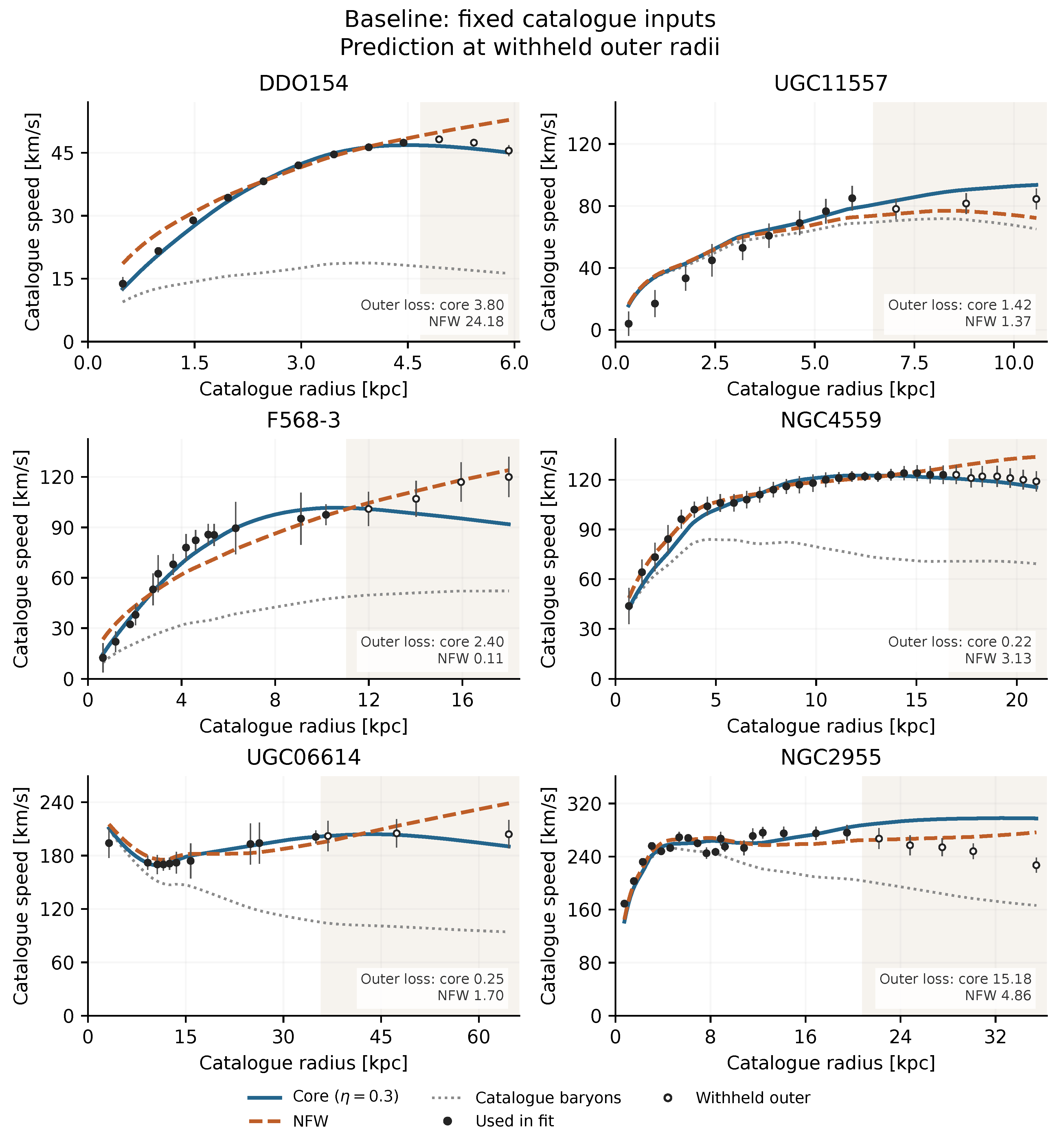
Figure 2.
Matched-nuisance predictions for the same six illustrative galaxies as Figure 1. Each model independently fits its permitted parameters and the common nuisance priors. The baryons-only curve is its own fitted prediction, not the baryonic contribution within another fit. Filled points train the fits; open points and shading mark withheld radii. Lines join saved predictions at observed radii. B and C cores each beat NFW in 4/6 displayed galaxies, versus 44/131 and 45/131 overall; the complete population appears in Figure 3. Point errors are observational, not predictive intervals.
Figure 2.
Matched-nuisance predictions for the same six illustrative galaxies as Figure 1. Each model independently fits its permitted parameters and the common nuisance priors. The baryons-only curve is its own fitted prediction, not the baryonic contribution within another fit. Filled points train the fits; open points and shading mark withheld radii. Lines join saved predictions at observed radii. B and C cores each beat NFW in 4/6 displayed galaxies, versus 44/131 and 45/131 overall; the complete population appears in Figure 3. Point errors are observational, not predictive intervals.
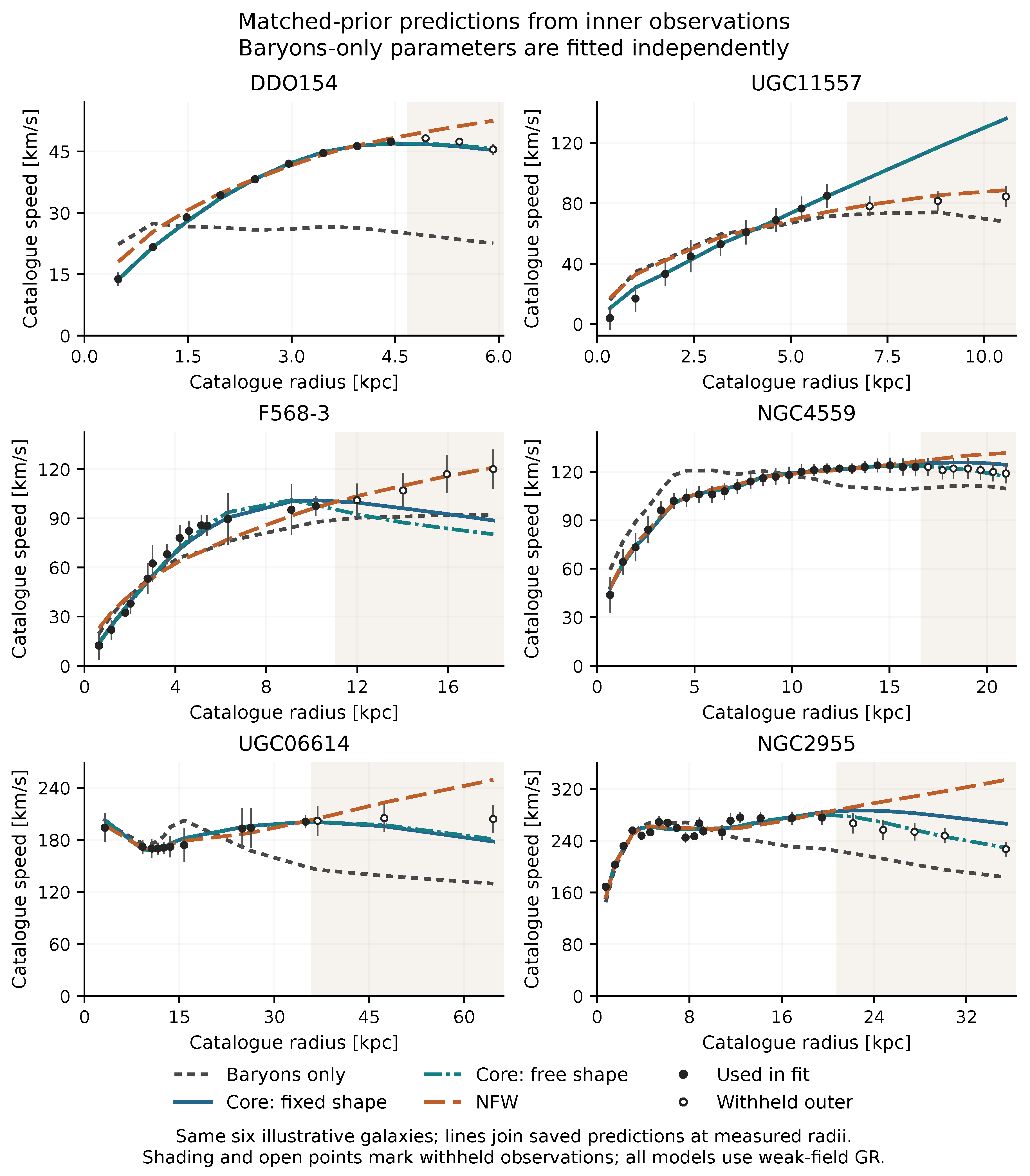
Figure 3.
Baryons-only and added-source predictions under the same weak-field GR equations. Rows compare fixed catalogue inputs and matched nuisance priors; columns distinguish all-radius agreement from inner-trained outer prediction. Each galaxy has equal weight. Curves further left have smaller loss; any infinite-loss case remains in the denominator and is shown at the separate infinity marker. B/C’s NFW predictions coincide. These empirical distributions are descriptive, not uncertainty bands. S17 gives failures, paired effects and the separately scoped five-comparison tests.
Figure 3.
Baryons-only and added-source predictions under the same weak-field GR equations. Rows compare fixed catalogue inputs and matched nuisance priors; columns distinguish all-radius agreement from inner-trained outer prediction. Each galaxy has equal weight. Curves further left have smaller loss; any infinite-loss case remains in the denominator and is shown at the separate infinity marker. B/C’s NFW predictions coincide. These empirical distributions are descriptive, not uncertainty bands. S17 gives failures, paired effects and the separately scoped five-comparison tests.
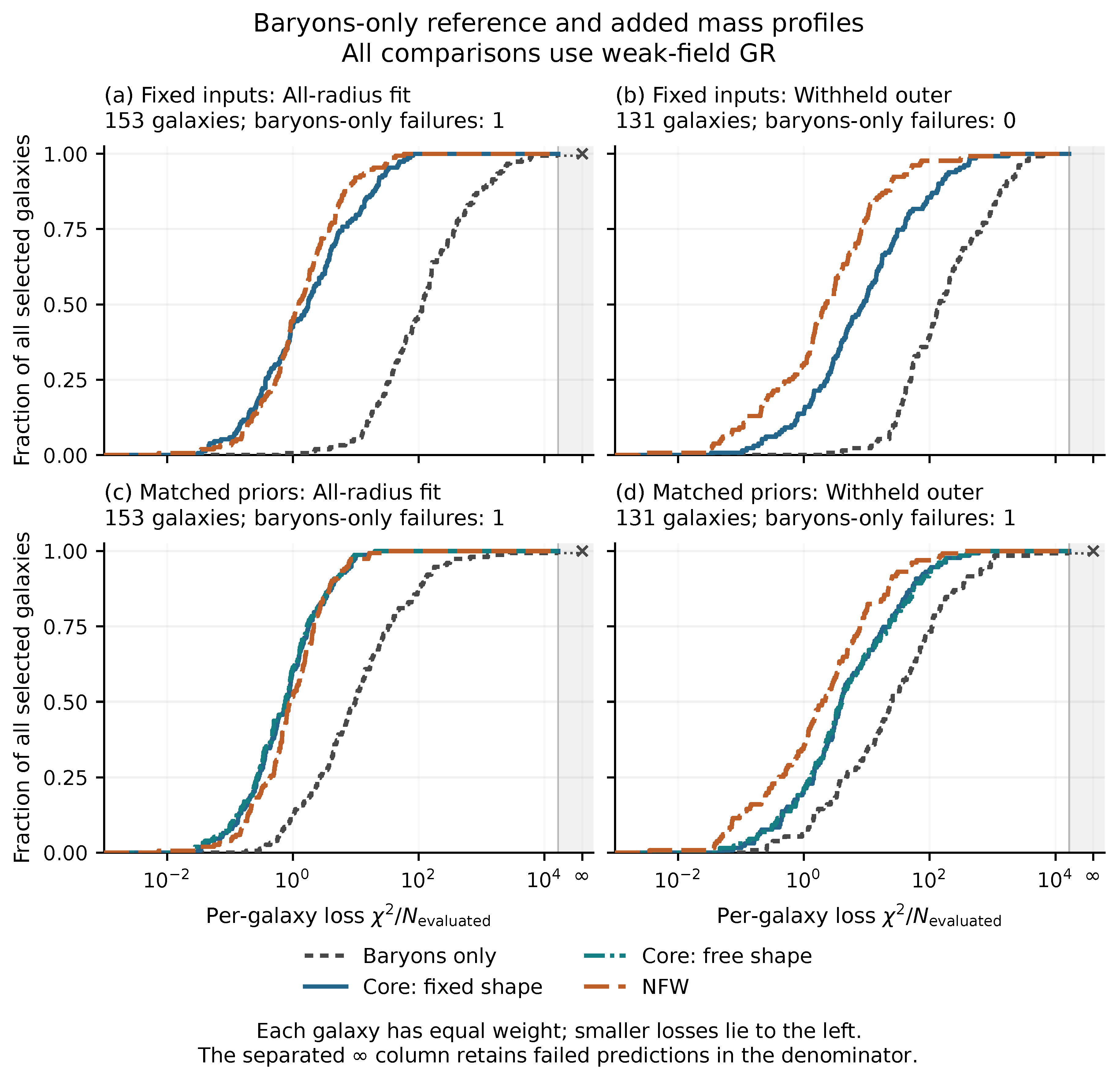
Figure 4.
Withheld outer prediction by catalogue morphology. Points give the left model’s fraction of galaxy wins; bars are marginal exact 95% binomial intervals, under independent galaxies with a common within-class win probability. Counts are wins/eligible galaxies; there are no ties or failed predictions. B and C use matched nuisance priors, with one extra core-shape parameter in C. Filled markers identify in the 60-test family, which also includes baseline A/NFW; the intervals are not simultaneous. Detailed types and overlapping broad groups are both shown; S0 appears in both partitions. Values above one half favor the left model in frequency, without establishing a lower mean loss. All fits remain isolated weak-field GR profile tests.
Figure 4.
Withheld outer prediction by catalogue morphology. Points give the left model’s fraction of galaxy wins; bars are marginal exact 95% binomial intervals, under independent galaxies with a common within-class win probability. Counts are wins/eligible galaxies; there are no ties or failed predictions. B and C use matched nuisance priors, with one extra core-shape parameter in C. Filled markers identify in the 60-test family, which also includes baseline A/NFW; the intervals are not simultaneous. Detailed types and overlapping broad groups are both shown; S0 appears in both partitions. Values above one half favor the left model in frequency, without establishing a lower mean loss. All fits remain isolated weak-field GR profile tests.
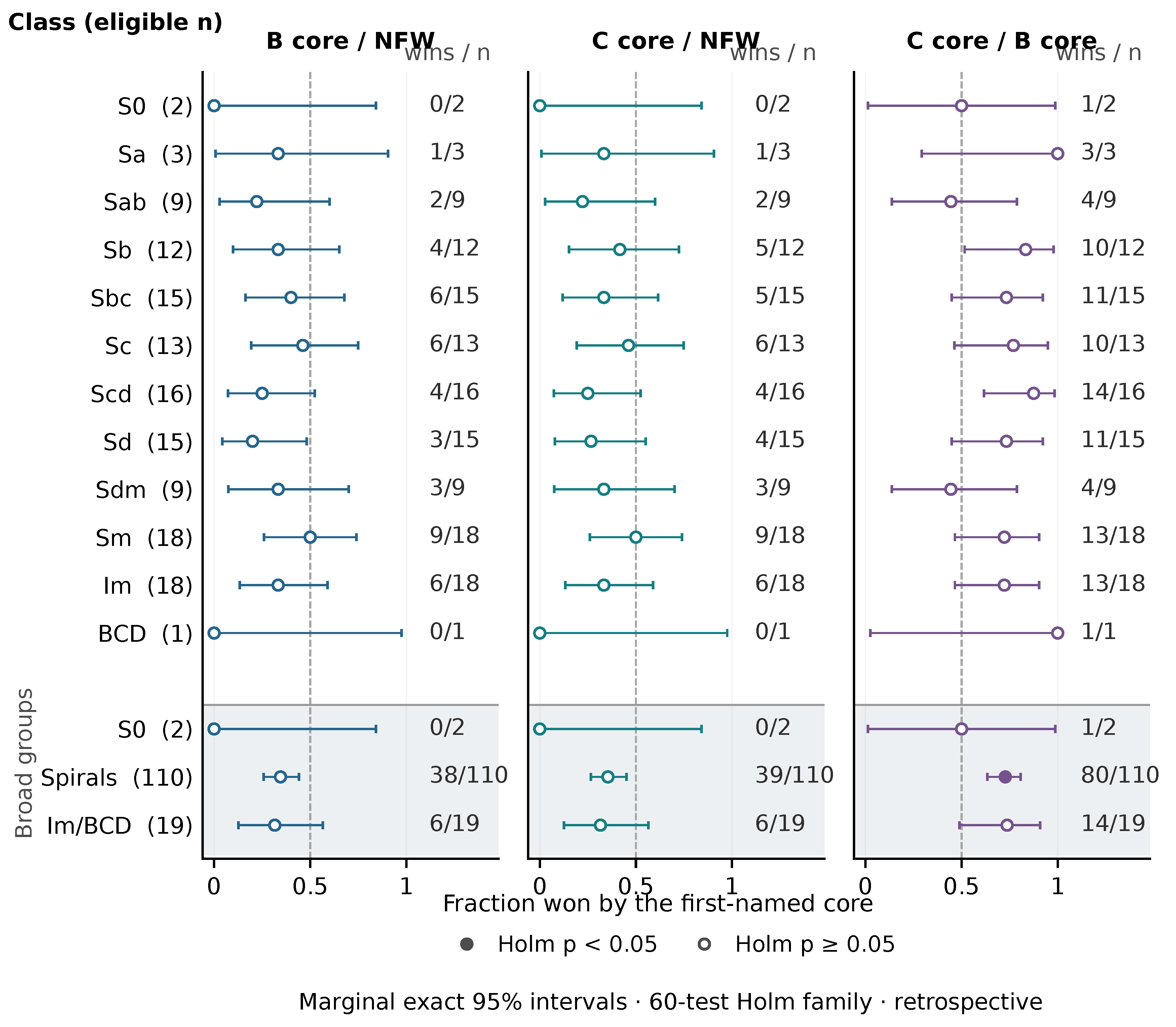
Figure 5.
Controlled two-field response with fixed microscopic coefficients and field number. Top: field-generated changes at , relative to the corresponding unrotated initial background for the baryonic switch, or unexcited stationary evolution for each imposed rotation. The common direct baryonic force cancels. Bottom left and right: internal gradient and excess contact energies after rotation by in the preferred/orthogonal spinor plane. Baryonic compression alone leaves both zero to numerical precision. Energies use . S16 documents the source, numerical convergence and separate passive-tracer response. These curves are controlled dynamics, not galaxy fits.
Figure 5.
Controlled two-field response with fixed microscopic coefficients and field number. Top: field-generated changes at , relative to the corresponding unrotated initial background for the baryonic switch, or unexcited stationary evolution for each imposed rotation. The common direct baryonic force cancels. Bottom left and right: internal gradient and excess contact energies after rotation by in the preferred/orthogonal spinor plane. Baryonic compression alone leaves both zero to numerical precision. Energies use . S16 documents the source, numerical convergence and separate passive-tracer response. These curves are controlled dynamics, not galaxy fits.
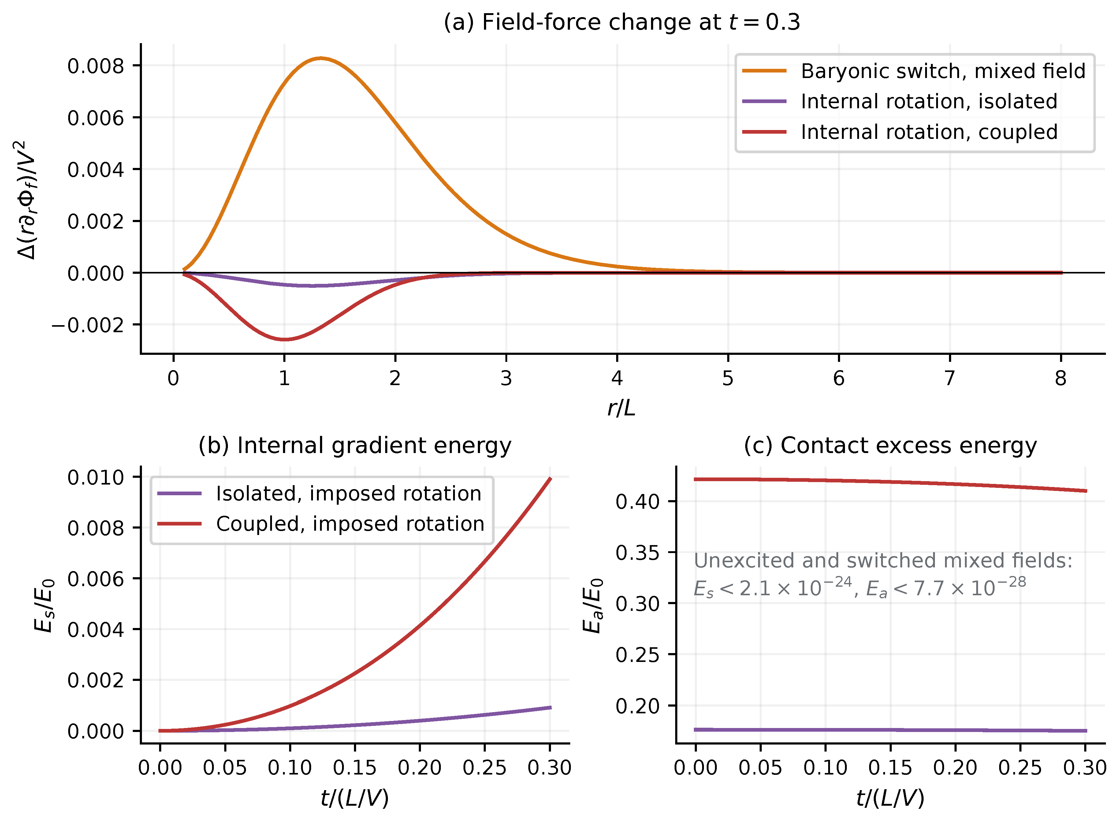
Figure 6.
Controlled equal-mass, zero-detuning comparison within the retained weak-field GR dynamics, for the specified theoretical rotation , . (a) Equal initial rest density gives exactly equal gravitational circular-speed curves. (b) The added internal stress supplies outward support to the field; passive tracers feel only the gravitational acceleration. (c) Self-consistent field evolution changes the potential; the normalized instantaneous squared-speed difference at and approaches the exact initial-time coefficient in (8.8). (d) The additional enclosed mass required to confine the unchanged profile returns toward zero; shaded radii require a negative added source density. All axes use the core scales . These are specified model calculations, not an observational estimate of internal stress.
Figure 6.
Controlled equal-mass, zero-detuning comparison within the retained weak-field GR dynamics, for the specified theoretical rotation , . (a) Equal initial rest density gives exactly equal gravitational circular-speed curves. (b) The added internal stress supplies outward support to the field; passive tracers feel only the gravitational acceleration. (c) Self-consistent field evolution changes the potential; the normalized instantaneous squared-speed difference at and approaches the exact initial-time coefficient in (8.8). (d) The additional enclosed mass required to confine the unchanged profile returns toward zero; shaded radii require a negative added source density. All axes use the core scales . These are specified model calculations, not an observational estimate of internal stress.
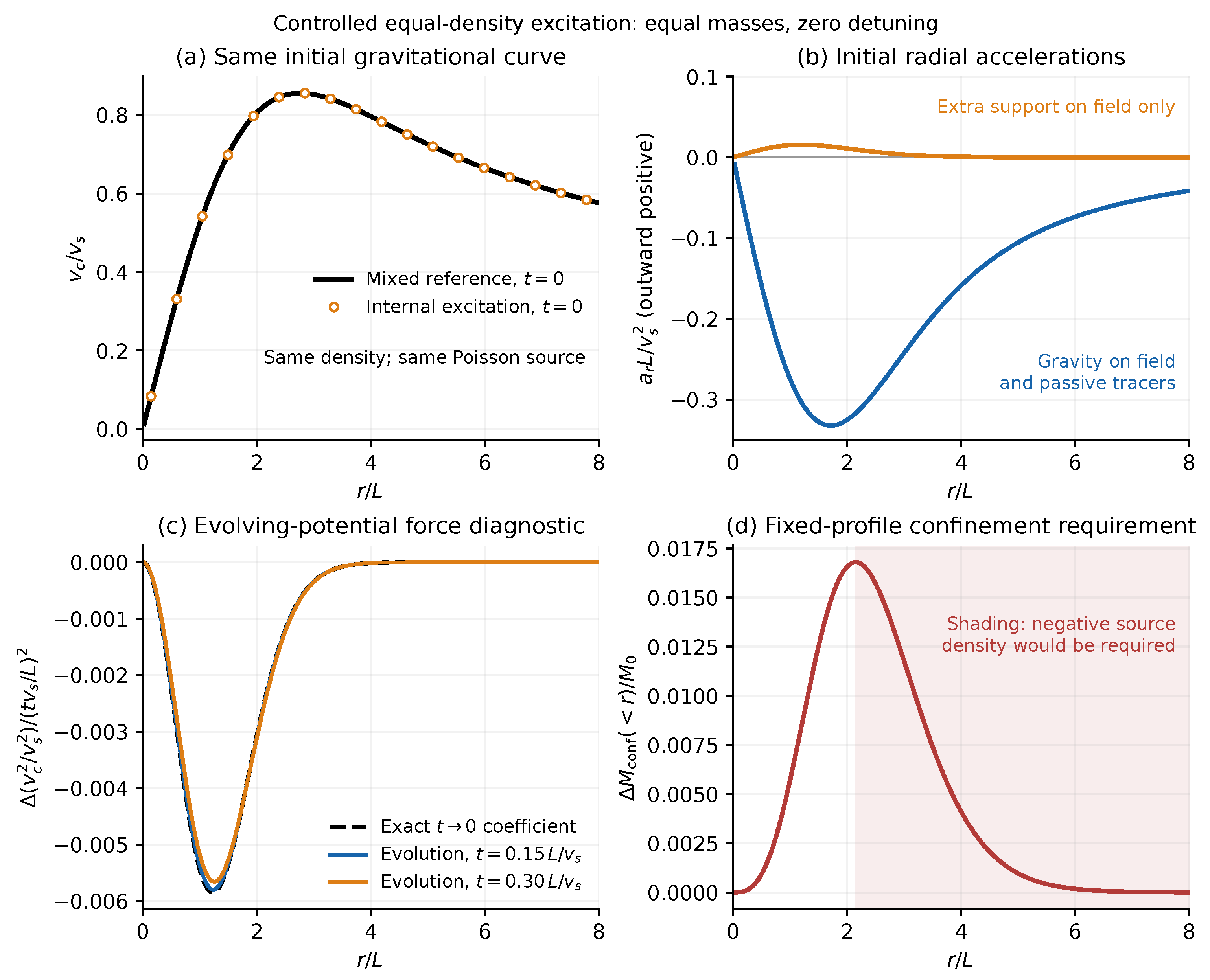
Figure 7.
Exact energy-channel consequences, evaluated without fitting. (a) Calibrated compression of the gradient and contact energies. (b) The normalized virial agrees with a numerical derivative of the register log partition function. (c) The variable-density isotropic family attains the unrestricted envelope; its pure-gradient endpoint is an unattained field limit. The star marks the exact fixed-positive-core value at , compared with the unrestricted . No intermediate fixed-core attainment is asserted; the dashed curve is a local quadratic approximation. (d) A separate disconnected compact equal-bump family keeps density, current and full momentum flux fixed while spanning at , and .
Figure 7.
Exact energy-channel consequences, evaluated without fitting. (a) Calibrated compression of the gradient and contact energies. (b) The normalized virial agrees with a numerical derivative of the register log partition function. (c) The variable-density isotropic family attains the unrestricted envelope; its pure-gradient endpoint is an unattained field limit. The star marks the exact fixed-positive-core value at , compared with the unrestricted . No intermediate fixed-core attainment is asserted; the dashed curve is a local quadratic approximation. (d) A separate disconnected compact equal-bump family keeps density, current and full momentum flux fixed while spanning at , and .
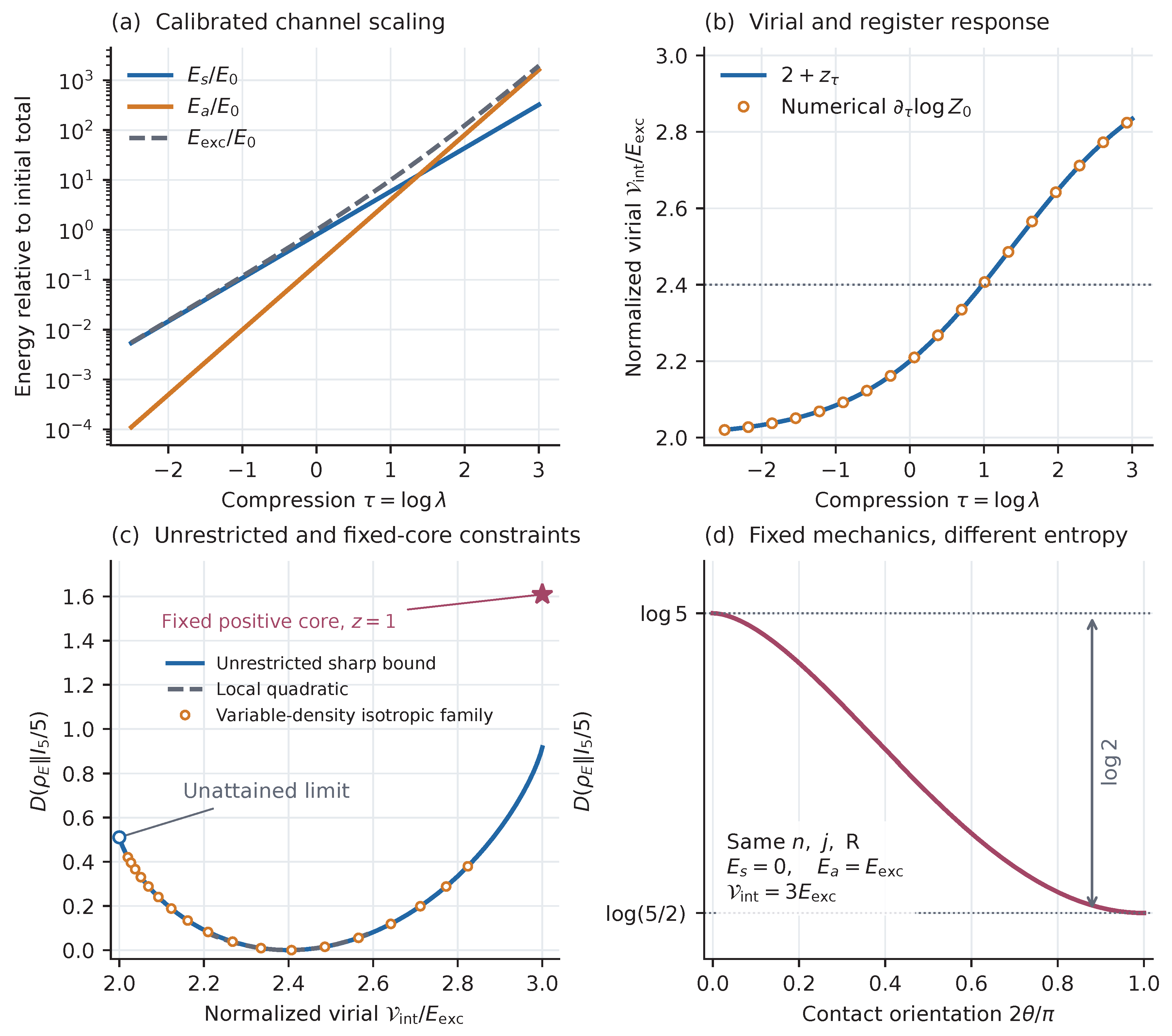

Table 1.
Consistent data losses for the fitted tiers. Full-data medians use 153 galaxies and 3168 rows; outer medians and galaxy-equal means use 131 separate inner-only fits and 659 withheld rows. Each loss is over the evaluated rows, not reduced chi-square or a penalized objective. C adds one core-shape parameter; its NFW fits are exactly B’s. All tiers share the guard.
Table 1.
Consistent data losses for the fitted tiers. Full-data medians use 153 galaxies and 3168 rows; outer medians and galaxy-equal means use 131 separate inner-only fits and 659 withheld rows. Each loss is over the evaluated rows, not reduced chi-square or a penalized objective. C adds one core-shape parameter; its NFW fits are exactly B’s. All tiers share the guard.
| Tier | Model | Full median | Outer median | Outer mean |
|---|---|---|---|---|
| A | Fixed core | 1.754 | 8.798 | 59.121 |
| A | NFW | 1.235 | 2.213 | 19.700 |
| B | Fixed core | 0.804 | 3.890 | 27.802 |
| B | NFW | 0.899 | 1.971 | 12.095 |
| C | Variable core | 0.756 | 4.039 | 28.836 |
Table 2.
Comparison under matched nuisance priors. Loss is , excluding prior penalties. Full-data medians use all 153 galaxies; outer summaries use 131 inner-trained predictions. The profiled baryons-only reference has one infeasible training case, assigned infinite loss; its medians remain finite. RMS is in . The last column counts outer wins against that reference.
Table 2.
Comparison under matched nuisance priors. Loss is , excluding prior penalties. Full-data medians use all 153 galaxies; outer summaries use 131 inner-trained predictions. The profiled baryons-only reference has one infeasible training case, assigned infinite loss; its medians remain finite. RMS is in . The last column counts outer wins against that reference.
| Source model | Full median | Outer median | Outer median RMS | Wins |
|---|---|---|---|---|
| Baryons alone | 9.908 | 24.458 | 24.18 | - |
| Baryons + B core | 0.804 | 3.890 | 10.11 | 101/131 |
| Baryons + C core | 0.756 | 4.039 | 9.72 | 99/131 |
| Baryons + NFW | 0.899 | 1.971 | 5.32 | 116/131 |
Table 3.
Reference core for the controlled dynamics. encloses 99% of the computed mass. These are model outputs, not measurements or fitted uncertainties.
Table 3.
Reference core for the controlled dynamics. encloses 99% of the computed mass. These are model outputs, not measurements or fitted uncertainties.
| Input | Value | Output | Value |
|---|---|---|---|
Disclaimer/Publisher’s Note: The statements, opinions and data contained in all publications are solely those of the individual author(s) and contributor(s) and not of MDPI and/or the editor(s). MDPI and/or the editor(s) disclaim responsibility for any injury to people or property resulting from any ideas, methods, instructions or products referred to in the content. |
© 2026 by the authors. Licensee MDPI, Basel, Switzerland. This article is an open access article distributed under the terms and conditions of the Creative Commons Attribution (CC BY) license (http://creativecommons.org/licenses/by/4.0/).
Copyright: This open access article is published under a Creative Commons CC BY 4.0 license, which permit the free download, distribution, and reuse, provided that the author and preprint are cited in any reuse.