
Submitted:
23 September 2026
Posted:
28 September 2026
You are already at the latest version
Abstract
Vibration-driven robots represent a lightweight and mechanically simple class of locomo tion systems that achieve propulsion through oscillation-induced frictional interactions with the ground, eliminating the need for wheels, legs, or tracks. Despite their promise for tasks such as in-pipe inspection, debris clearance, and small-scale medical operations, most existing models assume purely elastic coupling or linear viscous damping, thereby 1 2 3 4 5 6 neglecting complex dissipative phenomena. This study introduces and analyzes a two- 7 module vibration-driven robot in which the interconnecting element is a spring–damper 8 system filled with a non-Newtonian fluid. The effective damping in this configuration 9 is nonlinear and explicitly dependent on the angular velocity of the unbalanced rotating 10 mass, resulting in strong coupling between actuator dynamics and energy dissipation. A 11 set of governing dynamic equations is derived to capture these interactions and is validated 12 through numerical simulation. Parametric studies are conducted to quantify the influence 13 of design variables such as mass, stiffness, and fluid rheological properties on locomotion 14 velocity and energetic cost. The results demonstrate that nonlinear damping introduced by 15 non-Newtonian fluids significantly alters locomotion regimes, enabling adaptive trade-offs 16 between stability, efficiency, and speed. These findings highlight the potential of velocity- 17 dependent damping to enhance vibration-driven locomotion and provide new pathways 18 for the design and control of next-generation energy-efficient mobile robots.
Keywords:
vibration-driven robots
; non-Newtonian damping
; nonlinear dynamics
; locomotion efficiency
; spring–damper coupling
; multi-objective optimization
; energy-efficient robotics
1. Introduction
Vibration-driven robots are a class of locomotion mechanisms that utilize oscillatory motion to propel themselves across different surfaces [1,2]. Unlike conventional mobile robots that rely on wheels, legs, or tracks, vibration-driven robots exploit oscillation-induced frictional forces to generate net forward motion [3,4]. This principle eliminates the need for complex mechanical transmission systems and reduces structural redundancies, thereby making such robots simple to fabricate, lightweight, and cost-efficient [5,6]. Furthermore, vibration-driven robots can traverse diverse environments, including flat or inclined planes, rough terrains, and irregular surfaces, which highlights their versatility in both engineered and natural settings [8]. These attributes have positioned vibration-driven robots as attractive solutions for a range of tasks, such as post-disaster debris clearance, in-pipe inspection and maintenance, and even targeted medical applications at small scales [9,10,11].
A fundamental feature of vibration-driven robots is their reliance on internal oscillatory components, such as unbalanced rotating or reciprocating masses, piezoelectric actuators, pneumatic chambers, or electromagnetic drivers, to generate propulsion [12,13]. The locomotion efficiency of such robots strongly depends on how the oscillatory input energy is distributed and transformed into translational displacement through interactions with the ground [14]. An essential factor in this process is the coupling mechanism between different modules of the robot, which governs the exchange of energy and the resultant motion profile [15]. Most prior designs have relied on purely elastic coupling, typically springs, to connect modules. While springs can store and release oscillatory energy, they do not account for dissipative effects that naturally occur in real-world systems. This leads to simplified dynamics that may not capture the complex interplay between actuation, damping, and friction [16,17].
Previous research on vibration-driven robots has largely focused on simpler linear models. For instance, [11] analyzed a two-module vibration-driven system with elastic coupling and investigated the influence of friction asymmetry on net displacement. [7] derived governing dynamic equations for a two-body system connected by a spring and driven by unbalanced rotating masses, and validated their models with experiments. [3] explored dynamic modeling and open-loop control for two- and three-module vibration robots actuated by reciprocating internal masses, showing how excitation phase shifts affect steady-state velocity. [24] further analyzed locomotion due to stick–slip effects in two-module systems. While these studies provide valuable insight into the dynamics of vibration-driven systems, they all assume linear elastic coupling and neglect complex damping phenomena.
In order to more accurately represent and exploit such dynamics, damping mechanisms have been incorporated into various robotic systems. Conventional approaches often rely on linear viscous damping with constant coefficients [18,19,20]. However, in practice, damping is rarely linear, and materials or fluids often display nonlinear or rate-dependent behaviors. In particular, non-Newtonian fluids have emerged as a promising candidate for advanced damping applications [21]. Unlike Newtonian fluids, whose viscosity remains constant under varying shear rates, non-Newtonian fluids exhibit shear-dependent viscosity, which can be either shear-thinning (decreasing viscosity with increasing shear rate) or shear-thickening (increasing viscosity with shear rate) [22]. These unique rheological properties allow the design of damping elements whose resistance adapts dynamically to the excitation conditions [23].
Integrating non-Newtonian fluids into vibration-driven robots introduces a new paradigm in locomotion. When such a fluid is embedded in a damper connecting the robot’s modules, the effective damping becomes a nonlinear function of the excitation frequency and velocity. This provides a natural form of adaptive dissipation that can enhance stability, improve energy efficiency, or even generate novel locomotion regimes. Importantly, when the robot is actuated by an unbalanced rotating mass, the angular velocity of the rotor directly influences the shear rate in the non-Newtonian fluid, thereby coupling actuation and damping in a unique manner. As a result, the damping force is not only time-varying but also explicitly dependent on the actuator dynamics, creating a rich nonlinear interaction between oscillatory input, elastic restoring forces, nonlinear damping, and ground friction.
Some works have introduced damping explicitly but in linearized forms. [25] investigated single-module bristle-bots with unbalanced masses, analyzing velocity dependence on excitation and friction coefficients. [15] proposed a capsule-type vibration robot with an electromagnetic actuator and spring coupling, controlled via duty-cycle modulation. [26] presented a one-way wheeled vibration robot actuated by contra-rotating unbalanced masses, where locomotion efficiency was optimized near resonance frequencies. More recently, [5] conducted bi-objective optimization of a two-module vibration robot to simultaneously maximize forward velocity and minimize backward slip, using the NSGA-II algorithm [27]. Despite these advances, damping was always treated as either negligible or constant, leaving the potential of nonlinear, velocity-dependent damping largely unexplored.
The motivation of this work stems from these research gaps. Specifically, there has been limited exploration of how nonlinear damping, especially through non-Newtonian fluids, can influence the performance of vibration-driven robots. Given the strong velocity dependence of such fluids, incorporating them into spring–damper couplings offers the possibility of novel locomotion behaviors and enhanced energy efficiency. Moreover, when the damping characteristics are directly coupled to actuator velocity, the optimization and control strategies must be revisited, as linear assumptions no longer hold.
In this paper, we propose and analyze a two-module vibration-driven robot in which the modules are connected by a spring–damper system filled with a non-Newtonian fluid (as shown in Figure 1). The damper introduces nonlinear, velocity-dependent resistance that varies with the angular velocity of the unbalanced rotating mass. The governing dynamic equations are derived to capture this coupled nonlinear behavior, and the model is validated against numerical simulations. A parametric study is then conducted to assess the influence of key design variables, such as module mass, spring stiffness, and fluid properties, on the robot’s average velocity and energy consumption. Multi-objective optimization using NSGA-II is performed to determine parameter sets that maximize locomotion efficiency while minimizing energy use.
The main contributions of this work can be summarized as follows. First, we introduce a vibration-driven robot with a spring–damper coupling that incorporates a non-Newtonian fluid, resulting in nonlinear and velocity-dependent damping directly linked to the actuator dynamics. Second, we develop and validate governing dynamic equations that capture the interplay between elastic restoring forces, nonlinear damping, and frictional interactions with the ground. Third, we perform a multi-objective optimization of the robot parameters to simultaneously enhance locomotion velocity and reduce energy consumption.
This study advances the field of vibration-driven robotics by incorporating realistic nonlinear damping into the modeling and optimization framework, and by demonstrating that adaptive damping via non-Newtonian fluids can significantly influence locomotion performance and control.
2. Nonlinear Governing Equations of the Spring–Damper Coupled Robot
In this study, we investigate a vibration-driven modular robot composed of two rigid modules, denoted and , connected via a spring–damper element. The coupling mechanism consists of a linear elastic spring of stiffness k and initial rest length d, in parallel with a nonlinear damper containing a non-Newtonian fluid. The damping coefficient is a function of the angular velocity of an unbalanced mass m mounted on a rod of length L pivoted at the center of the front module. The angular position, velocity, and acceleration of this unbalanced mass are , , and , respectively. A schematic of the system is shown in Figure 2.
2.1. Assumptions and Modeling Considerations
To formulate the equations of motion, the following assumptions are made:
- 1.
- The rod carrying the unbalanced mass is considered massless, so its rotational inertia is negligible.
- 2.
- The modules are rigid, with equal masses .
- 3.
- The robot’s motion is constrained along a single horizontal axis, corresponding to translational locomotion.
- 4.
- Static and kinetic coefficients of friction are identical, , to simplify the frictional model.
- 5.
- The unbalanced mass is treated as a point mass, allowing simplification of the torque and centrifugal force expressions.
2.2. Horizontal Dynamics of the Front Module
Applying Newton’s second law in the horizontal direction to the front module yields the sum of all forces acting along the motion axis. These include the spring force, nonlinear damping, centrifugal and tangential contributions of the unbalanced mass, and the frictional resistance . Denoting the displacements of the front and rear modules as and , respectively, the governing equation reads:
The damping coefficient accounts for the non-Newtonian nature of the fluid. For a shear-thickening fluid, increases with , whereas for a shear-thinning fluid, it decreases. A commonly used model is:
where denotes the baseline viscosity-related parameter, is a scaling factor that modulates the degree of rate sensitivity, and defines the non-Newtonian regime, with corresponding to shear-thinning behavior and to shear-thickening behavior.
2.3. Vertical Equilibrium of the Front Module
The vertical forces acting on the front module consist of the module’s weight, the contribution of the unbalanced mass, and the normal reaction from the ground. To ensure continuous contact with the surface:
where g is the gravitational acceleration. This condition imposes bounds on the admissible angular velocity and acceleration of the rotor.
2.4. Dynamics of the Rear Module
The rear module experiences horizontal forces due to the spring, the nonlinear damper, and friction :
Its vertical equilibrium is trivial, as it does not carry the unbalanced mass:
2.5. Frictional Forces
The frictional forces acting on each module depend on the instantaneous motion state :
This piecewise definition ensures smooth transition from static to kinetic friction in simulations.
2.6. Matrix Form Representation
For compactness and suitability for numerical integration, the equations can be expressed in matrix form:
where
and
while the forcing vector is
2.7. Actuator Power and Energy Consumption
The instantaneous power delivered by the unbalanced rotating mass is
where the driving torque is
The total actuation energy consumed over a time interval is therefore
2.8. Remarks on Nonlinear Coupling
The velocity-dependent damping term introduces strong nonlinear coupling between the rotational actuation and translational locomotion. Unlike purely elastic couplings, this system exhibits frequency-dependent locomotion effi- ciency, which must be carefully considered in control and design. In subsequent sections, the validity of these govern- ing equations will be verified through numerical simulations.
3. Optimization of the Robot Parameters with Non-Newtonian Damping
The optimization framework is adapted to a robotic platform in which the inter-module coupling consists of a linear elastic spring arranged in parallel with a nonlinear, non-Newtonian damper. The damping coefficient is not constant, but instead exhibits a strong dependence on the rotor angular velocity, reflecting the rheological properties of shear-thinning or shear-thickening fluids. The velocity-dependent damping is described by Equation (2). This formulation enables a systematic investigation of how (), together with the actuation frequency, influence the trade-offs between locomotion efficiency, stability, and energy consumption.
3.1. Performance Metrics and Evaluation Protocol
The evaluation of locomotion performance is based on a set of metrics that quantify both efficiency and motion quality. The average forward velocity and total actuation energy are retained as primary indicators, while smoothness and contact integrity are included to capture the additional effects introduced by velocity-dependent damping:
where denotes the normal ground reaction force on the front module. The initial cycles of each simulation are discarded to eliminate transients, and metrics are computed over the subsequent cycles within the interval .
3.2. Constraints
The feasible design space is further delimited by physical and mechanical constraints to ensure model validity and hardware safety:
3.3. Non-Dimensional Formulation
To facilitate comparisons across a wide range of operating points, the system dynamics are reformulated in terms of dimensionless groups that naturally incorporate the non- Newtonian damping law:
With fixed, performance can thus be primarily mapped as a function of and , highlighting the interplay between stiffness, damping, and frequency.
3.4. Parametric Study
The influence of system parameters on locomotion performance is examined by considering their effects on , , and . The complete set of design variables is defined as
A Latin Hypercube Design (LHD) Viana, Venter and Balabanov (2010) of size is generated across prescribed parameter ranges:
For each sample, the governing equations introduced in Sec. 2 are integrated with the velocity-dependent damping model of (2), transients are discarded, and the performance metrics (14)–(17) are evaluated. The results are analyzed through: (i) main-effects plots of each parameter against and , (ii) sensitivity indices based on Sobol or Morris screening to rank parameter influence, and (iii) two- dimensional response maps in the space for fixed to reveal the frequency–damping interaction patterns.
3.5. Multi-Objective Optimization Problem
The optimization task seeks parameter configurations that achieve high forward speed with low energy consumption and smooth motion. This is formulated as a multi-objective problem:
where the box of admissible parameter bounds. For scalar selection of a single operating point, a weighted aggregate objective is considered:
with (, , ) determined by the relative priority of speed, energy, and smoothness.
3.6. Optimization Algorithm
A population-based evolutionary strategy (NSGA-II) Deb et al. (2002) is employed to approximate the Pareto front, as described in Giagkiozis and Fleming (2014), in the objective space (Vavg,Eact,Jrms). Due to the enlarged design space arising from the non-Newtonian damping law, surrogate models such as radial basis functions, such as Buhmann (2000), or Gaussian processes, such as Seeger (2004), are trained on the LHD dataset. These surrogates are used for iterative infill based on Expected Improvement (EI) to accelerate convergence. At prescribed intervals, selected candidate solutions are re-evaluated with the high-fidelity dynamics model to ensure accuracy and correct for surrogate bias.
3.7. Reproducibility
Reproducibility is supported by providing explicit bounds for all parameters, initialization seeds for the LHD design, solver tolerances, and post-processing routines for calculating , , and . This ensures that all reported Pareto sets and optimization results can be independently validated and replicated.
4. Results and Discussion
The joint influence of spring stiffness k, baseline damping , and rotor speed on the performance of the vibration–driven robot with non-Newtonian damping was evaluated numerically.
Representative time histories in Figure 3 show alternating stick–slip episodes and a persistent phase lead of the front module relative to the rear. The phase difference is central to net drift generation; it is amplified by appropriate stiffness and moderated by damping. No lift-off was observed at the operating point shown, consistent with the contact constraint satisfied in the simulations. The parameters are based on Table 1, where , , and .
Given that the overall damping factor is modeled as a function of the angular velocity , a comprehensive analysis was conducted to investigate how variations in influence key performance metrics of the robot. Specifically, the study examined the impact of changing angular velocity on drift velocity, total energy consumption, average power output, and the Cost of Transport (CoT). The CoT is a dimensionless parameter that quantifies the energy efficiency of locomotion, defined as the amount of energy required to move a unit mass over a unit distance.
To assess these effects, the angular velocity of the rotating mass was varied systematically from to . The results, illustrated in Figure 4a–d, indicate a clear trend: as the rotational speed increases, there is a corresponding rise in drift velocity, energy consumption, and average power. With the robot almost not moving at angular velocities below 20 , this behavior suggests that while higher angular velocities enhance the translational motion of the robot (as reflected in increased drift velocity), they do so at the cost of greater energy expenditure and power demands, thereby influencing the overall energetic efficiency of the system.
However, the CoT surface in Figure 4d presents a valley that aligns with the drift ridge but is shifted toward slightly higher damping, indicating that minimal transport cost occurs where forward rectification remains effective while excessive oscillatory energy is curtailed by damping. This valley provides a practical design corridor for energy–limited operation.
Figure 5 demonstrates the relationship between total energy consumption and stiffness (k) for two level of damping coefficients, low: and high: . For the lower damping coefficient (), total energy increases with stiffness, peaking around , and then slightly decreasing as stiffness continues to increase. This suggests that with lower damping, the robot requires more energy as stiffness increases, but it reaches a maximum energy consumption at a certain stiffness level. On the other hand, for the higher damping coefficient (), the total energy remains almost constant across the range of stiffness values, indicating that higher damping results in a more energy-efficient system, regardless of stiffness changes.
Figure 6 shows how drift velocity changes with stiffness for the same two damping values. For , drift velocity increases significantly with stiffness, peaking around before gradually decreasing with further increases in stiffness. This indicates that the robot’s drift velocity improves with higher stiffness up to a certain point, after which further stiffening has diminishing effects. However, for the higher damping coefficient (), drift velocity remains nearly constant across the range of stiffness values, showing that higher damping drastically reduces the impact of stiffness on the robot’s motion, resulting in a less responsive system.
Figure 7 illustrates the average power required for the robot as a function of stiffness. For the lower damping coefficient (), average power initially increases with stiffness, peaking and then decreasing at higher stiffness values, suggesting that maximum power consumption occurs at mid-range stiffness. In contrast, for the higher damping coefficient (), the power consumption remains steady across stiffness levels, indicating a stable but less efficient performance. This behavior highlights that while high damping can provide stability, it leads to a less efficient power usage, particularly as stiffness increases.
The results demonstrate that locomotion efficiency arises from a three–way balance between elastic energy storage, velocity–dependent dissipation, and friction–mediated rectification. Quantitative ranges extracted from the simulations indicate average power between – W and total actuation energy between – J across the domain considered, while the cost of transport (CoT) collapses by orders of magnitude once exceeds a threshold near 50 rad/s.
The surface in Figure 8a shows that average power generally increases with both k and , reflecting higher elastic forces and larger viscous losses. Non-monotonic regions appear where added damping stabilizes the stick–slip cycle and reduces wasted oscillation, producing shallow power minima for intermediate .
Figure 8b exhibits a more uniform rise of total energy with stiffness, consistent with the larger work required to sustain oscillations against a stiffer coupling. Increasing produces a gradual energy increase due to enhanced dissipation. Together, Figure 8a,b indicate that tuning stiffness and damping independently is suboptimal; instead, an intermediate band in delivers acceptable power and energy budgets while maintaining viable oscillation amplitudes.
The corresponding drift–velocity map shown in Figure 8c reveals a ridge at moderate stiffness and low-to-moderate damping. Insufficient damping results in nearly symmetric oscillations with limited rectification, whereas excessive damping suppresses oscillation amplitude and reduces stride length. The observed ridge therefore reflects the parameter combination that maximizes phase-lag asymmetry between the modules under Coulomb friction.
The Pareto set in Figure 8d captures the trade–off between speed and energy. Knee–point candidates provide balanced operating points with significant velocity gains for modest energy penalties. Coloring by n indicates that shear–thinning cases () populate the upper–left portion of the Pareto front, corresponding to higher velocity for a given energy expenditure, whereas shear–thickening cases () cluster toward lower velocity and higher energy regions. This trend is consistent with stronger rate–dependent damping at elevated angular velocities .
The results presented in Figure 10 illustrate the influence of the four key parameters on the average velocity and actual energy expenditure . The plots demonstrate that is relatively insensitive to variations in stiffness k, with most data points concentrated near zero regardless of the stiffness values, except for a few isolated outliers. In contrast, exhibits a clearer trend, where increasing frequency generally leads to higher values of , suggesting that oscillatory dynamics play a stronger role in enhancing system speed compared to stiffness adjustments.
Figure 9.
Main effects of model parameters on average velocity () and actual energy expenditure (). The top row illustrates the variation of with stiffness (k) and angular frequency (), whereas the bottom row shows the dependence of on the damping coefficient () and nonlinearity parameter (). The results indicate that is more sensitive to changes in than to variations in k, while exhibits greater variability with respect to both and , with occasional outliers influencing the observed trends. Overall, and appear to exert stronger influence on system performance than k and .
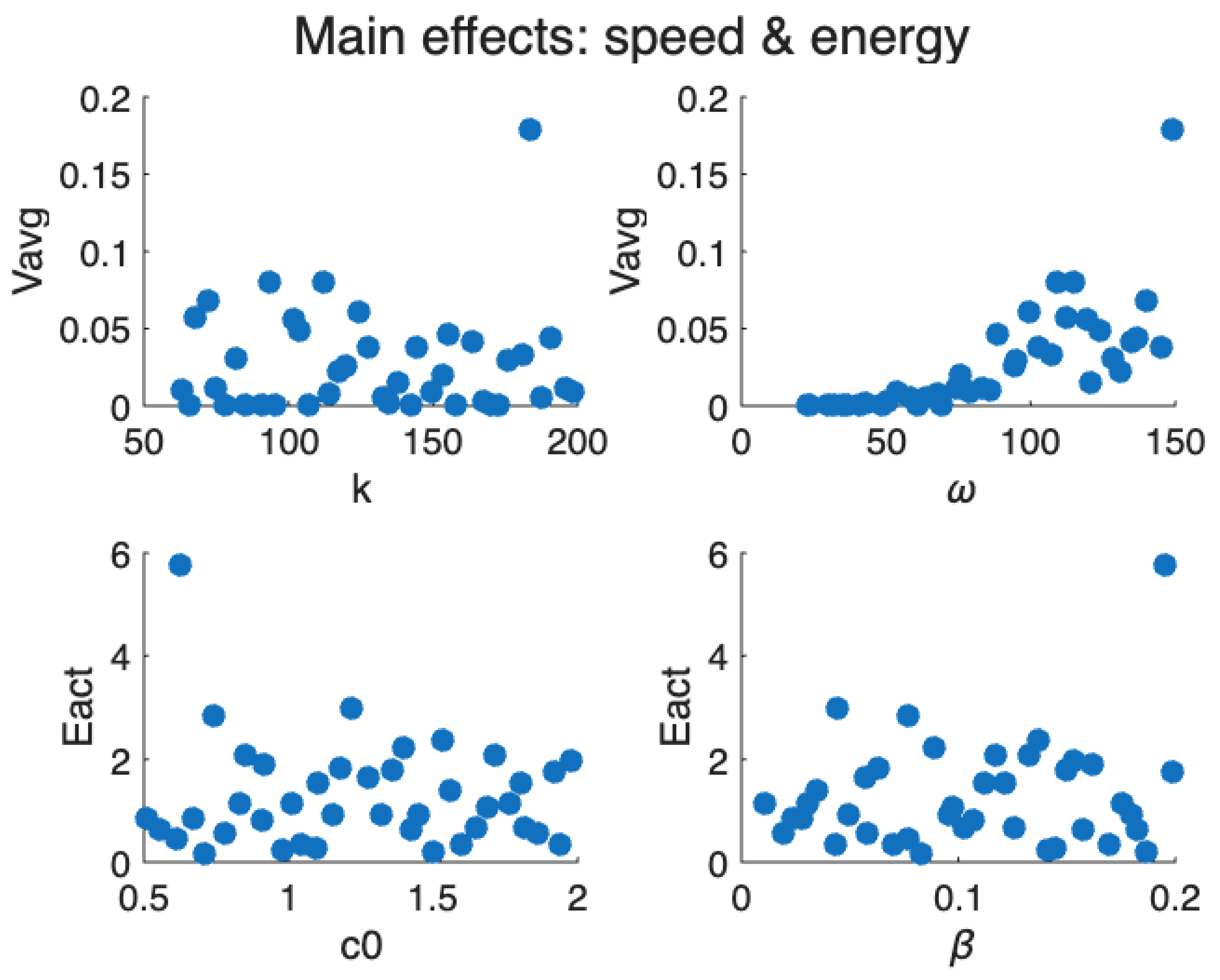
Figure 10.
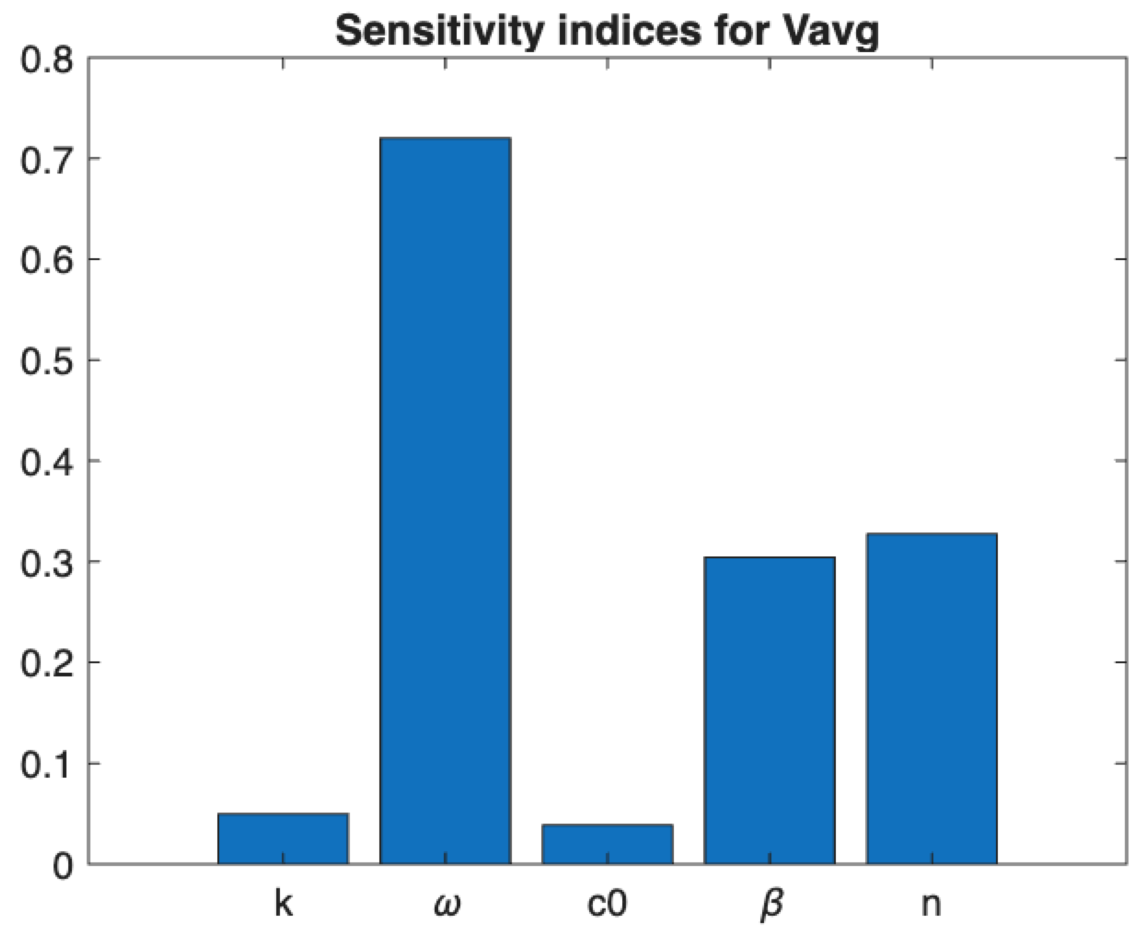
Correlation-based sensitivity of to ().
On the other hand, the energy expenditure does not exhibit a strong deterministic dependence on either or , as indicated by the scattered distributions. While appears to influence only weakly across its range, the effect of is slightly more pronounced, with occasional large increases in energy cost at higher values. These outliers suggest the possibility of nonlinear interactions or unstable operating regimes that may significantly elevate the energy requirements of the system.
These analyses highlight that while velocity performance is governed primarily by the oscillation frequency , energy expenditure is more susceptible to nonlinear effects associated with . This distinction implies that tuning is the most effective strategy for improving speed, whereas careful regulation of is crucial for maintaining energy efficiency.
Sensitivity analysis in Figure 10 ranks and k as the dominant contributors to drift velocity, with exerting a secondary influence and becoming influential primarily in the high–frequency regime where departs significantly from . Although correlation–based indices provide only a first–order ranking, the resulting hierarchy aligns with the underlying physical interpretation: frequency determines the stride cadence, stiffness governs oscillation amplitude and phase relationships, and damping shapes rate–dependent energy dissipation and symmetry breaking.
5. Conclusions and Future Work
The findings indicate that the locomotion efficiency of the proposed vibration–driven robot, consisting of two modules linked by a spring and a damper whose resistance depends on angular velocity, arises from a subtle balance among actuation frequency, stiffness, and nonlinear damping. At low frequencies, inefficient translation results from limited rectification and small displacements per cycle. As the frequency increases, rectification becomes more effective, leading to rapid growth in average velocity and a corresponding reduction in the cost of transport. Beyond a certain threshold, however, further increases in frequency amplify the rate–dependent damping, which curtails oscillation amplitude and limits additional gains in performance. This establishes a transition regime in which efficiency improves sharply before saturating at higher frequencies.
The interaction between stiffness and damping further refines this balance. Intermediate stiffness values provide sufficient compliance for displacement while avoiding excessive elastic energy storage that would otherwise increase the power requirement. Similarly, nonlinear damping modulates system performance depending on whether the fluid operates in a shear–thinning or shear–thickening regime. In shear–thinning fluids, reduced effective damping at moderate frequencies permits larger stride lengths and higher velocities without proportional increases in energy expenditure. Conversely, in shear–thickening regimes, frequency–dependent damping suppresses oscillations, enhancing stability but reducing drift velocity unless compensated through simultaneous adjustments in stiffness and actuation frequency.
Furthermore, the resulting Pareto front was visualized using color maps corresponding to either n (representing shear–thinning versus shear–thickening behavior) or (representing damping sensitivity). Candidate solutions were highlighted through weighted aggregation of objectives and by identifying knee–points along the Pareto front. Constraint activity, such as the proportion of time during which , was also evaluated to exclude operating conditions approaching ground–contact loss.
Theoretical arguments and simulation results revealed several characteristic trends. Increasing either or n enhances at elevated frequencies, which generally reduces oscillation amplitude and lowers , but also suppresses forward velocity unless is adjusted concurrently. In shear–thinning regimes (), moderate angular velocities result in lower effective damping, enabling larger stride lengths per actuation cycle and improved velocity at comparable energy expenditure. Consequently, the optimal combination of frequency and stiffness is not fixed, but shifts according to , highlighting the need for integrated co–design of stiffness and damping characteristics.
These findings establish a clear design principle: optimal locomotion emerges when the excitation frequency is tuned slightly above the rectification threshold, where net displacement increases more rapidly than energy cost, while material parameters are selected to balance compliance with controlled damping. This emphasizes the importance of co–design strategies that integrate actuation frequency with structural and rheological parameters to achieve efficient transport. Moreover, the identification of parameter regimes that naturally align high velocity with low energy expenditure provides a rational basis for guiding future experimental validation and practical implementation of non–Newtonian vibration–driven locomotion systems.
References
- Xu, J.; Fang, H. Improving performance: Recent progress on vibration-driven locomotion systems. Nonlinear Dyn. 2019, 98, 2651–2669. [Google Scholar] [CrossRef]
- Cocuzza, S.; Doria, A.; Reis, M. Vibration-based locomotion of an amphibious robot. Appl. Sci. 2021, 11, 2212. [Google Scholar] [CrossRef]
- Zhan, X.; Xu, J.; Fang, H. A vibration-driven planar locomotion robot—Shell. Robotica 2018, 36, 1402–1420. [Google Scholar] [CrossRef]
- Notomista, G.; Mayya, S.; Mazumdar, A.; Hutchinson, S.; Egerstedt, M. A study of a class of vibration-driven robots: Modeling, analysis, control and design of the brushbot. Proc. IEEE/RSJ Int. Conf. Intelligent Robots and Systems (IROS), 2019; pp. 5101–5106. [Google Scholar]
- Diao, B.; Zhang, X.; Fang, H.; Xu, J. Optimal control of the multi-module vibration-driven locomotion robot. J. Sound Vib. 2022, 527, 116867. [Google Scholar] [CrossRef]
- Reis, M.; Cocuzza, S.; Doria, A.; Adar, N.G. Vibration-based robot locomotion. Front. Robot. AI 2024, 11, 1508130. [Google Scholar] [CrossRef] [PubMed]
- Zimmermann, K.; Zeidis, I.; Bolotnik, N.; Pivovarov, M. Dynamics of a two-module vibration-driven system moving along a rough horizontal plane. Multibody Syst. Dyn. 2009, 22, 199–219. [Google Scholar] [CrossRef]
- Becker, F.; Lysenko, V.; Minchenya, V.T.; Kunze, O.; Zimmermann, K. Locomotion principles for microrobots based on vibrations. In Microactuators and Micromechanisms; Springer, 2016; pp. 91–102. [Google Scholar]
- Diao, B.; Zhang, X.; Xu, J. The optimal control methodology based on normalized Gaussian functions for vibration-driven locomotion robots. Multibody Syst. Dyn. 2024, 1–20. [Google Scholar] [CrossRef]
- Zhou, W. Design of oscillatory movement for ground-based locomotion and synchronized movement in bioinspired robotics; University of California: San Diego, 2022. [Google Scholar]
- Bolotnik, N.N.; Zeidis, I.M.; Zimmermann, K.; Yatsun, S.F. Dynamics of controlled motion of vibration-driven systems. J. Comput. Syst. Sci. Int. 2006, 45, 831–840. [Google Scholar] [CrossRef]
- Sabbadini, A.; Atalla, M.A.; Wiertlewski, M. Simple and fast locomotion of vibrating asymmetric soft robots. Soft Robot. 2023, 10, 1199–1208. [Google Scholar] [CrossRef] [PubMed]
- Schonebaum, J.K.; Alijani, F.; Radaelli, G. Review on mobile robots that exploit resonance. Proc. Inst. Mech. Eng. Part C 2021, 235, 7907–7924. [Google Scholar] [CrossRef]
- Korendiy, V.; Krot, P.; Kachur, O.; Predko, R.; Lanets, O. Influence of the imbalanced rotor and supporting surface inclination angles on locomotion characteristics. In Design, Simulation, Manufacturing; Springer, 2025; pp. 98–109. [Google Scholar]
- Bolotnik, N.N.; Nunuparov, A.M.; Chashchukhin, V.G. Capsule-type vibration-driven robot with an electromagnetic actuator and an opposing spring. J. Comput. Syst. Sci. Int. 2016, 55, 986–1000. [Google Scholar] [CrossRef]
- Amiri, N.; Sohrabi, K.; Eftekharian, G.; Fakhari, V. Optimization and control of an energy-efficient vibration-driven robot. J. Vib. Control 2024, 30, 2184–2199. [Google Scholar] [CrossRef]
- Mousavi, S.M.; Fakhari, V. Design and development of closed-loop controllers for trajectory tracking. J. Vib. Control 2024, 10775463241276026. [Google Scholar] [CrossRef]
- Biglari, H.; Golmohammadi, M.; Hayati, S.; Hemmati, S. Vibration reduction of a flexible robot link using a frictional damper. J. Vib. Control 2021, 27, 985–997. [Google Scholar] [CrossRef]
- Zhan, X.; Xu, J. Locomotion analysis of a vibration-driven system with three acceleration-controlled internal masses. Adv. Mech. Eng. 2015, 7, 1687814015573766. [Google Scholar] [CrossRef]
- Abas, Z.; Kim, H.S.; Zhai, L.; Kim, J. Finite element analysis of vibration-driven electro-active paper energy harvester. Adv. Mech. Eng. 2015, 7, 1687814015571231. [Google Scholar] [CrossRef]
- Chhabra, R.P. Non-Newtonian fluids: An introduction. In Rheology of Complex Fluids; Springer, 2010; pp. 3–34. [Google Scholar]
- Partal, P.; Franco, J.M. Non-newtonian fluids. Rheol. EOLSS 2010, 96–119. [Google Scholar]
- Irgens, F. Rheology and Non-Newtonian Fluids; Springer, 2014. [Google Scholar]
- Chen, Q.; Xu, J. Locomotion of two vibration-driven modules connected by a mechanical position limiter. Int. J. Mech. Sci. 2018, 137, 252–262. [Google Scholar] [CrossRef]
- Becker, F.; Lysenko, V.; Minchenya, V.; Zeidis, I.; Zimmermann, K. An approach to the dynamics of a vibration-driven robot. In ROMANSY 19; Springer, 2013; pp. 299–306. [Google Scholar]
- Loukanov, I.; Vitliemov, V.; Stoyanov, S.; Stoyanov, S. Design developments of vibration-driven mobile robots. Proc. 56th Science Conf. Ruse University, 2017; pp. 50–59. [Google Scholar]
- Deb, K.; Pratap, A.; Agarwal, S.; Meyarivan, T. A fast and elitist multiobjective genetic algorithm: NSGA-II. IEEE Trans. Evol. Comput. 2002, 6, 182–197. [Google Scholar] [CrossRef]
- Giagkiozis, I.; Fleming, P.J. Pareto front estimation for decision making. Evol. Comput. 2014, 22, 651–678. [Google Scholar] [CrossRef] [PubMed]
- Buhmann, M.D. Radial basis functions. Acta Numer. 2000, 9, 1–38. [Google Scholar] [CrossRef]
- Seeger, M. Gaussian processes for machine learning. Int. J. Neural Syst. 2004, 14, 69–106. [Google Scholar] [CrossRef] [PubMed]
- Viana, F.A.C.; Venter, G.; Balabanov, V. An algorithm for fast optimal Latin hypercube design. Int. J. Numer. Methods Eng. 2010, 82, 135–156. [Google Scholar] [CrossRef]
Figure 1.
CAD model of the proposed vibration-driven robot with a spring inside a cylinder filled with non-Newtonian fluid (top) and cross-sectional view of the robot (bottom).
Figure 1.
CAD model of the proposed vibration-driven robot with a spring inside a cylinder filled with non-Newtonian fluid (top) and cross-sectional view of the robot (bottom).
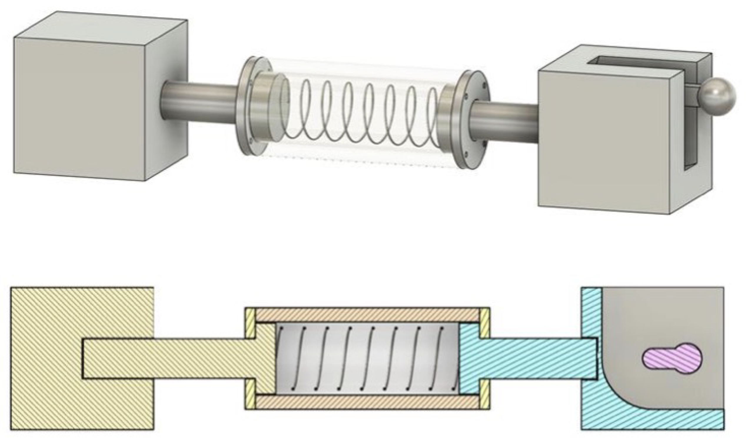
Figure 2.
Schematic of vibration-driven robot with damping as a function of angular velocity of the rotating mass.
Figure 2.
Schematic of vibration-driven robot with damping as a function of angular velocity of the rotating mass.
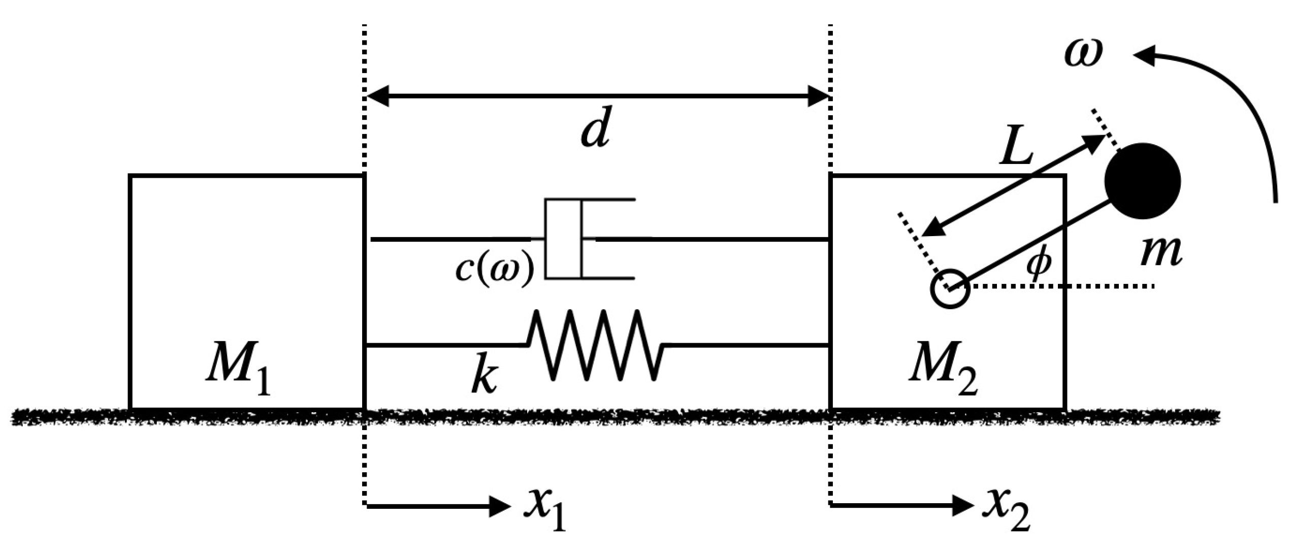
Figure 3.
Representative time histories of positions and velocities at an operating point near the CoT valley. Alternating stick–slip and a consistent phase lead of the front module are evident.
Figure 3.
Representative time histories of positions and velocities at an operating point near the CoT valley. Alternating stick–slip and a consistent phase lead of the front module are evident.
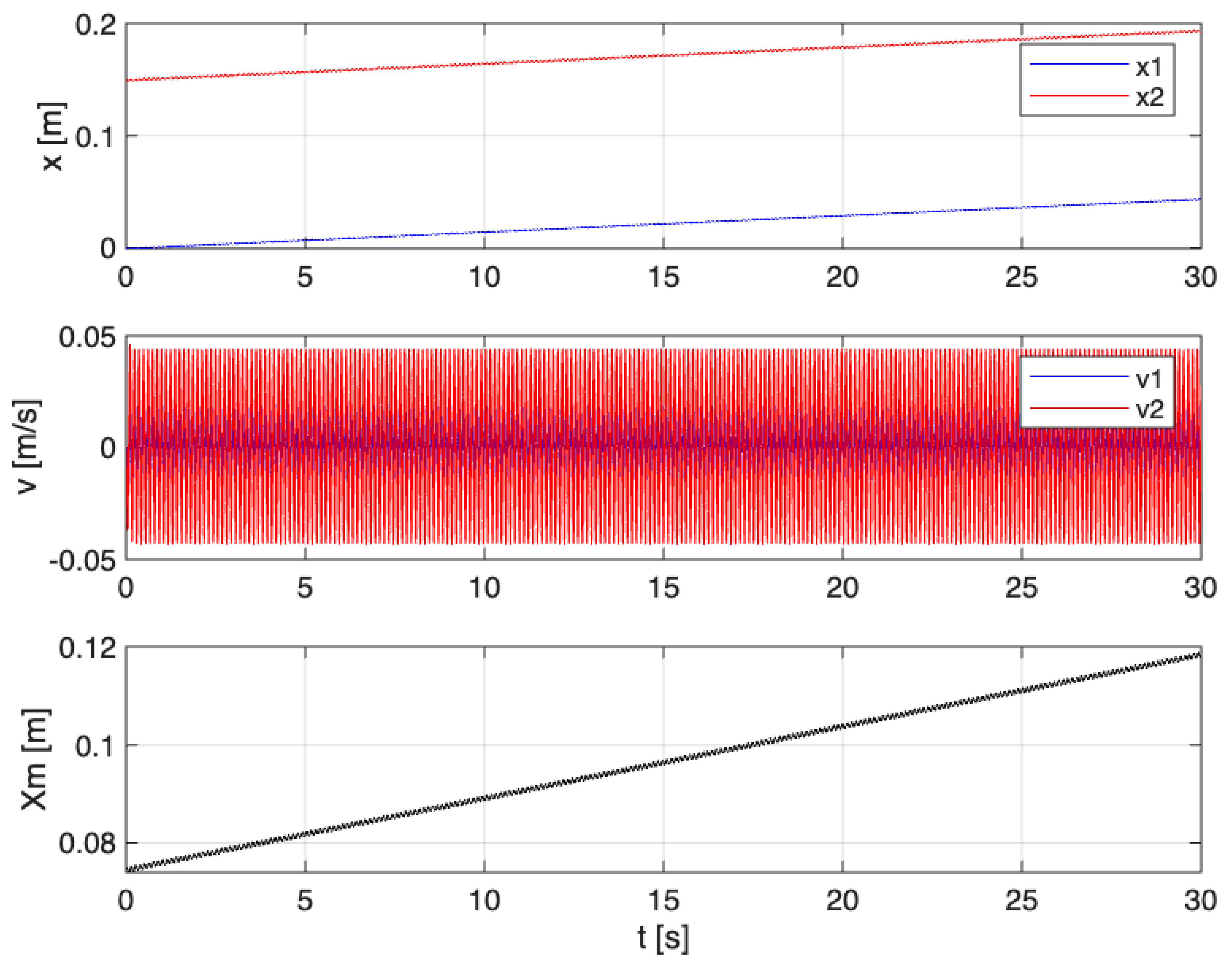
Figure 4.
Effects of angular velocity and system parameters on locomotion performance metrics.
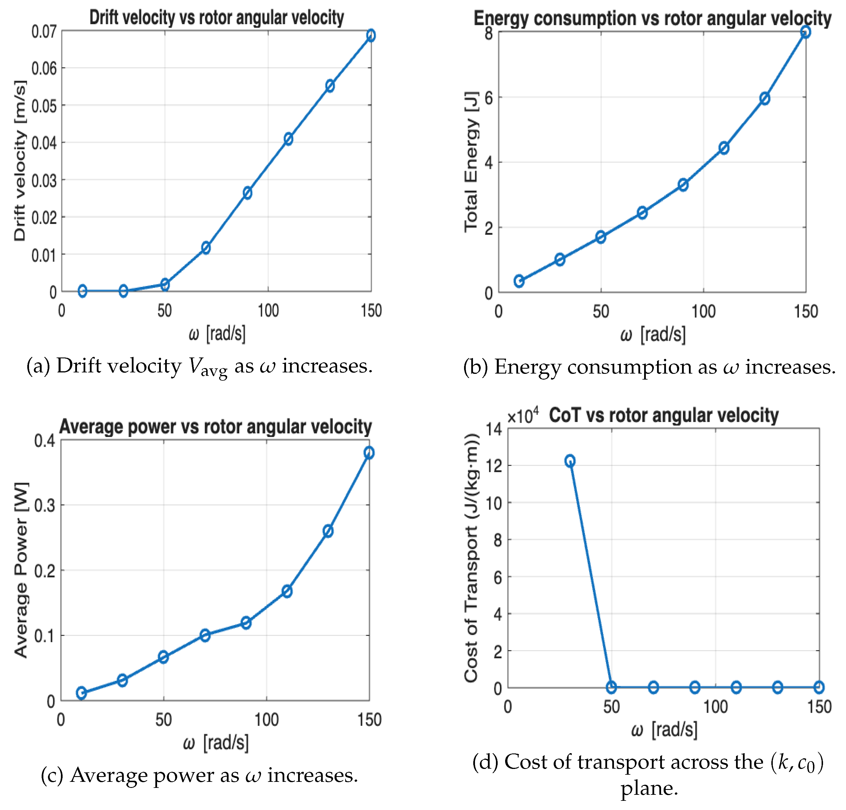
Figure 5.
Total energy consumption versus stiffness for low and high base damping coefficients ( and ). The graph illustrates how energy consumption increases with stiffness for the lower damping coefficient and remains almost constant for the higher damping coefficient.
Figure 5.
Total energy consumption versus stiffness for low and high base damping coefficients ( and ). The graph illustrates how energy consumption increases with stiffness for the lower damping coefficient and remains almost constant for the higher damping coefficient.
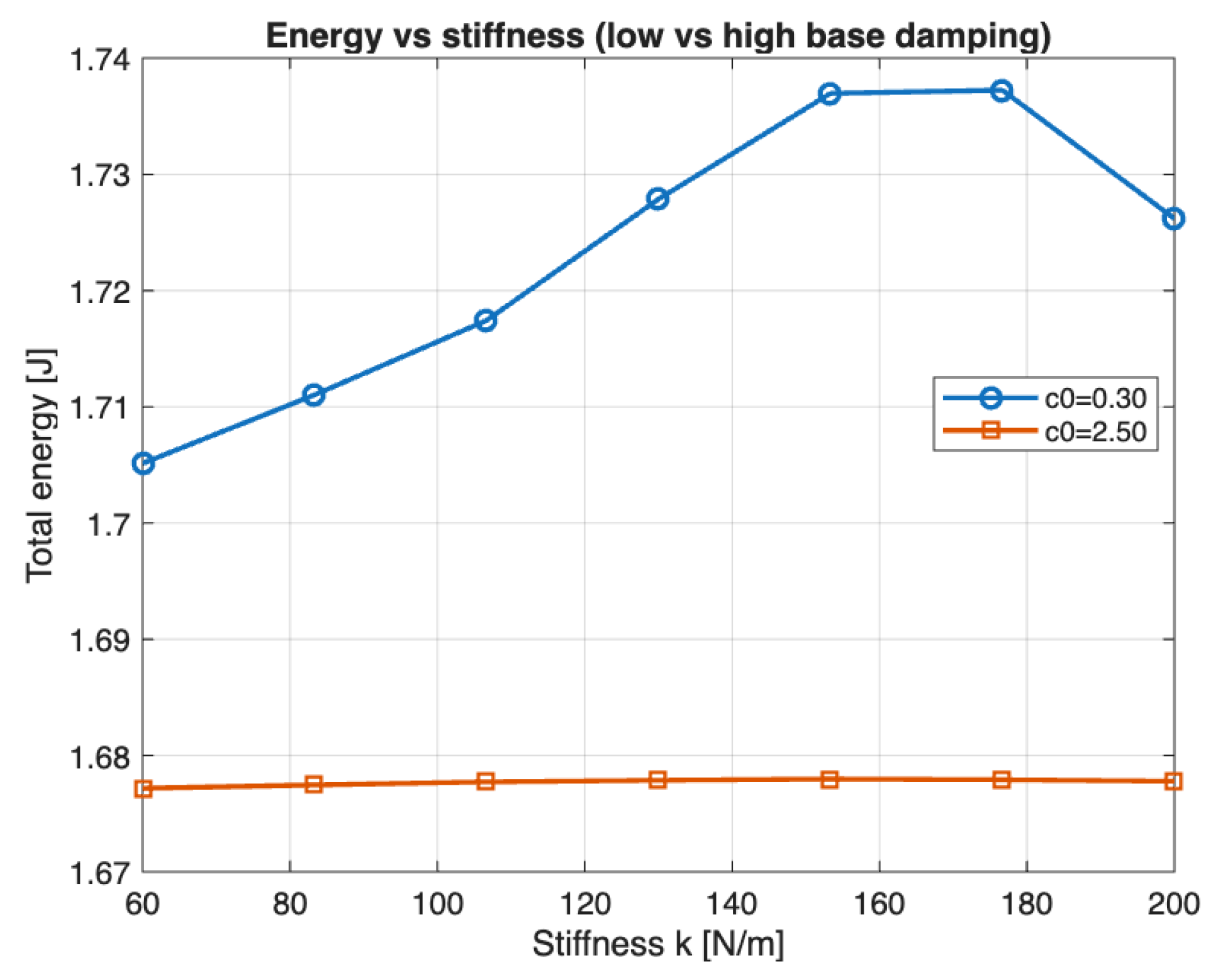
Figure 6.
Drift velocity versus stiffness for low and high base damping coefficients ( and ). The graph shows a significant increase in drift velocity with stiffness for the lower damping coefficient, peaking at around , while the higher damping coefficient shows a constant drift velocity.
Figure 6.
Drift velocity versus stiffness for low and high base damping coefficients ( and ). The graph shows a significant increase in drift velocity with stiffness for the lower damping coefficient, peaking at around , while the higher damping coefficient shows a constant drift velocity.
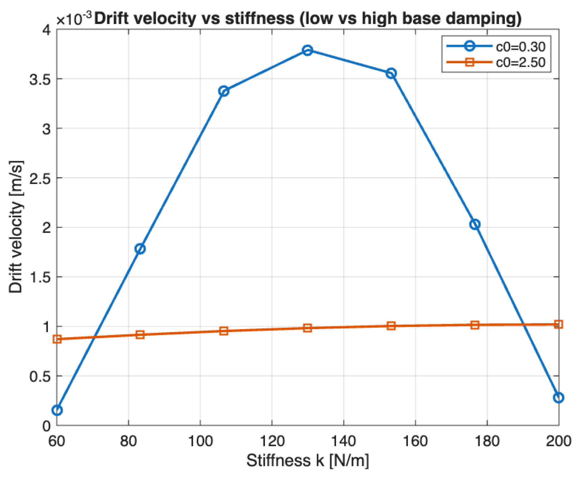
Figure 7.
Average power consumption versus stiffness for low and high base damping coefficients ( and ). For lower damping, average power increases with stiffness and peaks at mid-range values, while the higher damping coefficient shows stable power consumption across all stiffness levels.
Figure 7.
Average power consumption versus stiffness for low and high base damping coefficients ( and ). For lower damping, average power increases with stiffness and peaks at mid-range values, while the higher damping coefficient shows stable power consumption across all stiffness levels.
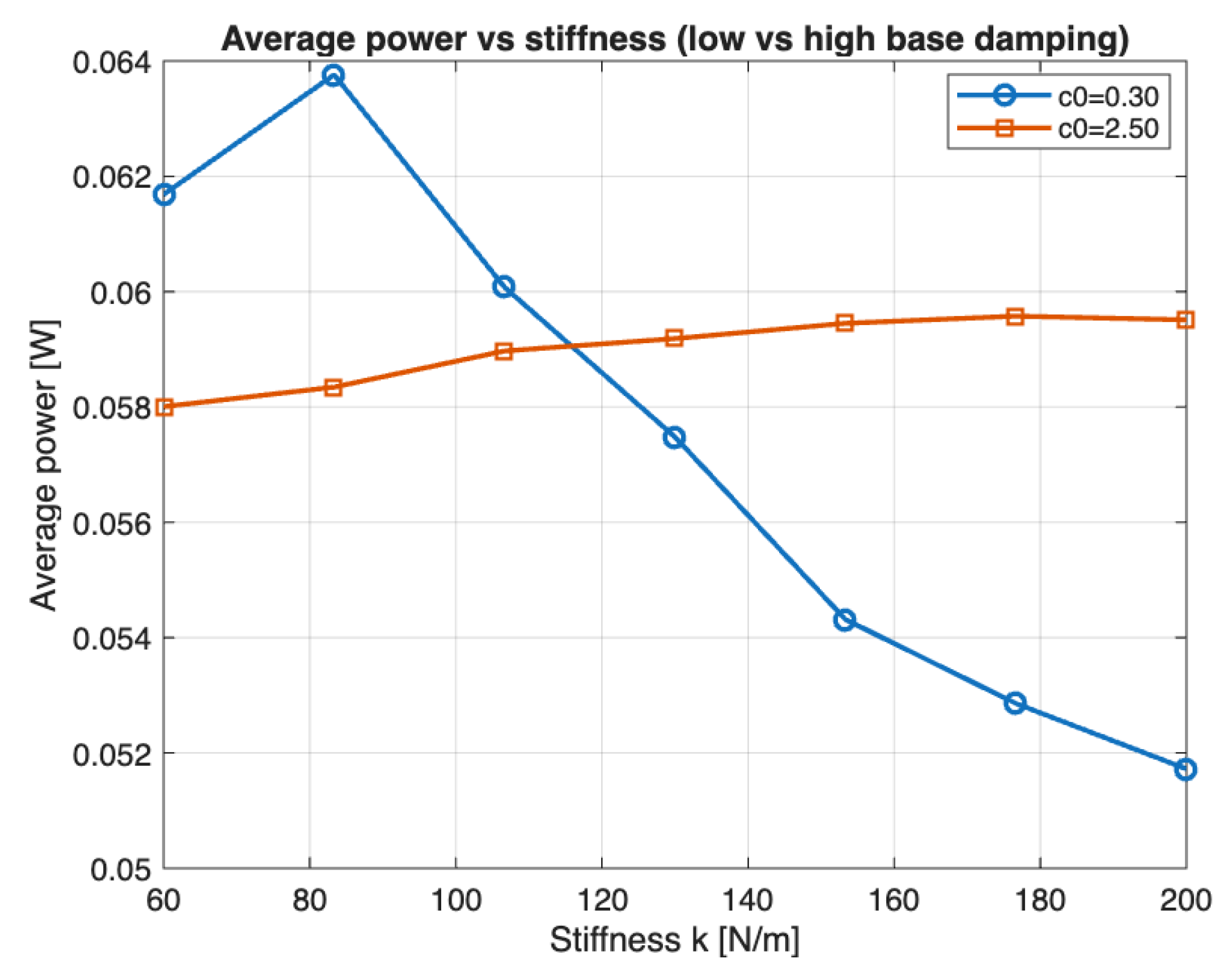
Figure 8.
Performance landscapes and optimization results: (a) average power surface, (b) total actuation energy surface, (c) average drift velocity surface, and (d) Pareto front illustrating the trade-off between drift velocity and energy expenditure.
Figure 8.
Performance landscapes and optimization results: (a) average power surface, (b) total actuation energy surface, (c) average drift velocity surface, and (d) Pareto front illustrating the trade-off between drift velocity and energy expenditure.
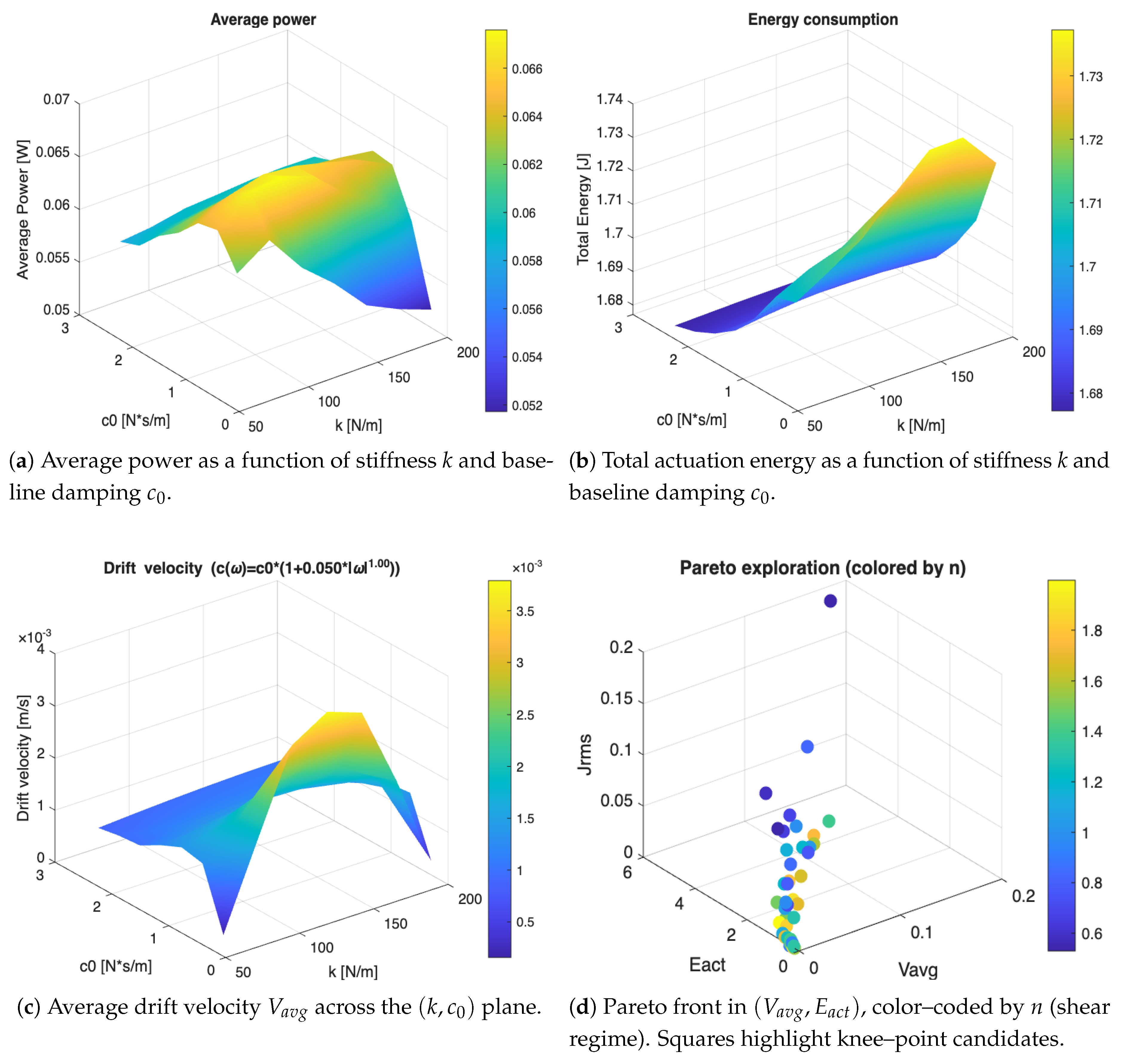

Table 1.
System parameters used in the simulations.
| Parameter | Unit | Value |
|---|---|---|
| M | kg | |
| m | kg | |
| L | m | |
| k | N/m | 130 |
| rad/s | 50 | |
| rad/s2 | 0 | |
| rad | ||
| d | m | |
| — | ||
| g | m/s2 | |
| N/ms | ||
| n | — | |
| — |
Disclaimer/Publisher’s Note: The statements, opinions and data contained in all publications are solely those of the individual author(s) and contributor(s) and not of MDPI and/or the editor(s). MDPI and/or the editor(s) disclaim responsibility for any injury to people or property resulting from any ideas, methods, instructions or products referred to in the content. |
© 2026 by the authors. Licensee MDPI, Basel, Switzerland. This article is an open access article distributed under the terms and conditions of the Creative Commons Attribution (CC BY) license (http://creativecommons.org/licenses/by/4.0/).
Copyright: This open access article is published under a Creative Commons CC BY 4.0 license, which permit the free download, distribution, and reuse, provided that the author and preprint are cited in any reuse.