
Submitted:
24 September 2026
Posted:
28 September 2026
You are already at the latest version
Abstract
The Brinkman equation provides a convenient continuum description of flow through digital cores containing resolved pores, unresolved porous voxels, and solids. Nevertheless, two issues are usually encountered in explicit solvers. The first is the instability in the discrete form of the viscous term when the porosity is violently changing. The second is the extremely small time-step restriction resulting from the stiff Darcy drag. This study addresses the two issues by developing a weakly compressible smoothed particle hydrodynamics (WCSPH) formulation in which the variable-porosity viscous term is expanded and its velocity-linear contribution is combined with the Darcy drag. The instability in the discrete formulation after this operator reorganization is greatly mitigated. For moderately stiff drag, the Strang splitting method with an exact integration of the drag is used to get rid of the drag restriction to the time step. Hence, the timestep is considerably enlarged. For severely stiff drag, the particle is integrated exactly with the enlarged timestep after neglecting the viscous contribution. A local selector based on the local Darcy number chooses between the two integration schemes. Constant-porosity channel tests show errors below 8% over the investigated parameter range, while variable-porosity channels, periodic porous obstacles, and two digital-core examples demonstrate numerical feasibility.
Keywords:
Brinkman equation
; weakly compressible SPH
; stiff drag
; Strang splitting
; exact integration
; digital core
; bulk permeability
1. Introduction
In-depth understanding of fluid flow in multiscale porous media is always required in engineering including but not limited to oil and gas recovery [39,40], carbon sequestration [32,33,34,37,38] and geothermal production [31,35,36]. Porous media in applications of these fields are considered as multiscale because the pores, throats and fractures in them usually span of a wide range in scale, from nanometers to micrometers and from several micrometers to millimeters. Numerical simulations are powerful tools to investigate the characteristic of the flows in these multiscale porous media. However, the classical pore scale simulations by solving the Navier-Stokes equation need too much detailed geometry of pores in all scales of the porous media of interest. Therefore, they require tremendous computational resources to implement the simulation and is impractical in application. A more realistic method is to model the porous media of interest with a properly chosen scale, which depicts the main structure of the porous media with resolved big pores and solid walls on one hand, and hides minor pore-solid structures below that scale in unresolved pixel or voxel on the other. Meanwhile, the sub-grid geometry and flow features in the unresolved pixels or voxels are extracted in terms of the local porosities and the local permeabilities. This procedure is accomplished via industrial microcomputed tomography (). Under a chosen scan resolution, the converted the porous structure of a piece of mineral core into a digital core of 3D CT values. The digital core is further segmented into ternary components, consisting of the pure pore domains for big pores, the unresolved domains for minor pore-solid structures, and the pure solid domains for solid walls [25]. Fluids which flow through the pure pore and the unresolved domains, bounded by the pure solid domains, are controlled by the Brinkman equation [1,20]. This equation is a generalization of the Navier-Stokes equation by adding a linear dragging force term with respect to the velocity. The dragging term depicts the friction between the fluid and the solid within the unresolved domains, and vanishes in the pure pore domains where the Brinkman equation reduce to the Navier-Stokes equation. In the unresolved domains, the strength of dragging is controlled by the permeability to porosity ratio. When the ratio is high, the dragging term is weak and the Brinkman equation falls to the Navier-Stokes limit; when the ratio is low, the flow is dragging force dominant and the Brinkman equation approaches to the Darcy flow limit. Therefore, the Brinkman equation is a perfect model to characterize multiscale porous flows with automatic scaling behavior. One thing is noted that near the Darcy flow limit, both the porosity and permeability are very low, the porous media is pretty like a solid wall and the dragging force becomes so strong to freeze any movement immediately. In this case, numerical simulation becomes difficult. Because the strong force needs to be resolved by a fine enough spatial solution, otherwise it becomes a stiff force numerically. The stiffness of the dragging force is controlled by the local Darcy number, which we define as the quotient of the permeability to porosity ratio over the resolution squared. As the local Darcy number decreases, the stiffness of the dragging force appears increasingly severe. This usually causes that the numerical solutions strongly deviate from correct solutions or even diverge. We will get back to the local Darcy number later when discussing integration scheme.
Numerical methods for the Brinkman equation are either explicit or implicit. The most frequently applied implicit solver for the Brinkman equation is the PIMPLE solver [24], which combines the PISO (Pressure Implicit Splitting Operator) algorithm [22] and the SIMPLE (Semi-Implicit Method of Pressure-Linked Equations) algorithm [21,23] to simulate the transient velocity field of the Brinkman equation. The PIMPLE solver is a finite volume method (FVM) type of algorithm designed for incompressible flows, in which the divergency of the velocity field must be zero. So, solving for the demanding Poisson pressure equation is required at each time step. This means the PIMPLE solver is both computationally expensive and memory demanding as the number of control volume is growing huge in 3D cases. Alternatively, the explicit methods normally close the momentum equation by an equation of state (EOS). This means solving the Poisson pressure equation is unnecessary and the solver is weakly compressible but fast in time integration. The lattice Boltzmann method (LBM) [16] is one of the typical weakly compressible methods, which has two models especially designed for porous flow, namely, the Gray model LBM [13,14] and the Brinkman force LBM [15,17,18]. The Gray model adds a “partial bounce-back” step in the unresolved domains after the “streaming” and “collision” steps of the classical LBM for modeling the resistance from the sub-grid solid to the flow. This model is subject to the fixed permeability-solid fraction relationship, from which the local permeability is binding to the local porosity. The Brinkman force model directly incorporates the linear dragging term of the Brinkman equation into the classical LBM body forcing. Thus, this model solves the Brinkman equation in the same way as solving the Navier-Stokes equation with a specific body force. Though, both of the LBM models show very high efficiency, their shortcomings are apparent as well. Firstly, the fixed permeability-solid fraction relationship is inconsistent to the real digital core. Moreover, the Gray model is subject to numerical inconsistency due to spurious flow oscillation and viscosity dependent permeability. The Brinkman force model, though suffers from less severe inconsistency, is incorrect when the local Darcy number mentioned above is low. This is because the forcing in LBM uses central scheme, which is only valid when the varying of the force is moderate during one time step. But the typical case of a digital core is that the unresolve domain has very low local Darcy number, which results in a stiff rapidly decaying dragging force. In this case, the central scheme forcing in LBM is unacceptable.
The smoothed particle hydrodynamics (SPH) method [2] is another computational fluid dynamics (CFD) method quite different from FVM and LBM. Essentially, it is a many-body particle dynamics simulator under the Lagrangian coordinate system for a broad range of physical phenomena, including the astrophysics [3], the fluid dynamics [27] and the solid mechanics [4]. In fluid dynamics, SPH uses a bunch of regularly distributed particles to represent the fluid and the solid boundary. The field qualities, such as the velocity, the density and the pressure of the fluid, at any specified position, are interpolated through integration of the quantity with a pre-defined kernel function. During simulation, the velocity and the position of each fluid particle are updated with a time integration scheme. This scheme is either explicit or implicit, depending on the choice of the method to close the momentum equation. The WCSPH [5] uses an EOS and is an explicit method. The incompressible SPH (ISPH) [6,7] requires the velocity divergence equal to zero and is a semi-implicit method. At early stage, both WCSPH and ISPH were blamed for its low accuracy due to tensile instability [4,5], which results in particle clumping and forming void regions. This was largely mitigated by using particle shift technique [7,8] or transport velocity correction scheme [9,10,11]. Meanwhile, as the incorporation of the low dissipation Riemann solver [12] into the community of SPH, the accuracy of both WCSPH and ISPH are apparently improved. But SPH is still rarely utilized in solving the Brinkman equation for evaluating the permeability of digital cores. The reason is that on one hand, as an implicit method, ISPH has no advantage over PIMPLE; on the other, as an explicit method, the conventional WCSPH is still highly inefficient, since the time step is extremely small when the local Darcy number tends to zero in the unresolved domains, where the local porosity and permeability are both very low. Recently, we discovered that the tiny time step issue of WCSPH method for the Brinkman flow can be tackled through a modified scheme. This will encourage the application of the powerful WCSPH method in broader applications.
This paper first expands the variable-porosity viscous term of the Brinkman equation. The velocity-linear contribution is combined with the Darcy drag, and a non-negative limiter is introduced when the combined coefficient becomes negative. This formulation stabilized viscous term when the porosity is violently changing. We then address the small timestep restriction of conventional WCSPH. The Strang splitting method is used along with an exact integration for the drag subproblem when the drag stiffness is moderate. The new integration scheme enables the usage of a considerably larger constrained only by the CFL number, the viscosity and the global maximum acceleration. In strongly drag-dominated regions, the viscous term is neglected and an exact integration scheme is used with the larger timestep. A local criterion based on the local Darcy number selects the integration scheme for each particle. The numerical study evaluates constant-porosity accuracy and demonstrates the behavior of the formulation in variable-porosity and digital-core configurations.
The remainder of this paper is organized as follows. Section 2 presents the reorganized Brinkman equation, the corresponding WCSPH spatial discretization, and the details of the two stiff-drag integration strategies. Section 3 reports channel-flow tests, periodic porous-obstacle examples, and 2D and 3D digital-core demonstrations. Section 4 discusses the scope, limitations, and further validation required for quantitative permeability prediction.
2. Materials and Methods
2.1. The Brinkman Equation
The Brinkman equation in the Eulerian form is written as Eq. (1) [1,41].
where is the flow velocity, is the external acceleration, is the density of the fluid, is the pressure of the flow, is the dynamic viscosity of the fluid. and are two position-based functions of the porous media, representing the local porosity and the local permeability, respectively.
In designed testing porous flow problems, the image of the porous media of interest is well segmented into three categories, representing the pure pores, the unresolved regions and the pure solid, where values of the porosity and the permeability are imposed for each pixel (in 2D) or each voxel (in 3D). However, in the real porous flow problems for a digital core, the CT values (or reduced CT values) of the porous media along with the resolution , are all we have at hand. Thus, it is necessary to discuss a little bit about how we obtain the local porosity and the local permeability from the CT values.
In order to obtain the local porosity, we need to know the bulk porosity of the core and this is down by experiment at large. Then, assuming the density and the effective atomic number of each mineral in the unresolved domain are similar, we use a truncated linear function to model the CT value to pixel (in 2D) or voxel (in 3D) porosity relationship, in Eq. (2) [25]:
where and are the threshold CT values for segmenting pure pore domains and pure solid domains, respectively. We can set and adjust the two threshold values with the help of any visualization software, by ensuring the averaged porosity equal to the bulk porosity of the core. For instance, Figure 1 shows that the blue region with low CT value represents the pure pore domain, the red region with high CT value represents the pure solid domain, and the region with gradually changing colors from blue to red represents the unresolved domain with sub-grid porous structure.
In order to obtain the local permeability, we select a few positions of the core with different porosities, drill the core at these positions for little cuts, scan the cuts with a much finer resolution by a CT device, segment the scanned CT imaging for binary structure containing only pores and solid, compute the porosity of each cut. Then, we have two methods for the permeability of each cut. The slower method is to use the pore-scale CFD simulation to solve the Navier-Stokes equation for the averaged velocity in the cut and then compute the permeability with Darcy’s law. The faster method is to use the pore-morphology method to compute the pore size distribution of the cut, compute the weighted average pore diameter of the cut with the pore size distribution, and then use Eq. (3) [25,26]:
to approximate the permeability of the cut. The limiter in Eq. (3) ensures when . Once the permeability of the cuts with different porosities are available, we can interpolate or fit a curve for the local porosity-permeability relation, then locate permeability value for each voxel is obtained.
Back to the Brinkman equation, the Eulerian form of Eq. (1) can be rewritten in the Lagrangian form as Eq. (4):
where , . The viscous term in Eq. (4) can be split into three terms as Eq. (5):
This formulation has two meanings in physics. The first is to provide viscous dissipation to the flow. The second is to make disturbance when the fluid flows through the porous region with varying porosities. When is a spatial constant, the formulation reduces to the normal viscous term as in the Navier-Stokes equation. When is spatially varying, the second and the third term in Eq. (5) start to disturb the flow field. It is noticed that the second term contains derivatives of velocity, which is similar to the first term. Whereas the third term is linear in velocity, which is in accordance with the dragging force term. Therefore, we reorganize the Brinkman equation by absorbing the third term of Eq. (5) into the dragging force as Eq. (6):
where, is the coefficient of the dragging force. Though is dominant in the coefficient for most cases, the use of limiter ensures that the dragging term is absolutely dissipative. We use the artificial equation of state in Eq. (7) to close Eq. (6).
where is the sound speed and is the reference density. We set , where is the maximum expected speed of the flow, to suppress the pressure oscillation down to below 1%. Since, the continuity equation is not directly solved in the chosen WCSPH formulation, where density is evaluated by interpolation with the kernel function and the mass conservation is strictly guaranteed, Eq. (6) and Eq. (7) are the equations we are solving for the rest of the paper. In order to estimate the bulk permeability of the digital cores, we use the no-slip boundary condition at the solid walls and periodic boundary condition at the physical boundary of the digital cores.
2.2. The Classical WCSPH of the Brinkman Equation
2.2.1. The WCSPH Formulation
For a digital core with pure pore domains, unresolved domains and pure solid domains, each pixel (in 2D) or voxel (in 3D) is initially assigned a particle at the center position of its cell. The particles in pure solid domains are labeled as fixed solid particles, and the rest particles are labeled as fluid particles. Each fluid particle interacts with its neighboring fluid particles and solid particles within the range of the support of its kernel function , where is the position of particle . One can be chosen any positive function with compact support as the kernel function . Here, we use the Wendland C2 function [28,29] in Eq. (8) as the kernel function:
where , is the smoothing length deciding the influence range of the kernel function. Here, 2 times the CT imaging resolution is used as the smoothing length, namely, . The coefficient in 2D, and in 3D, to ensure the exact integration of is unity. The density of particle is evaluated by the interpolation in Eq. (9):
where is the mass of the fluid particle, , where and , particle is located in the support of . The density of all solid particles is . The SPH discretization of Eq. (6) is Eq. (10):
where and are the acceleration of particle due to the pressure force, the viscous force and the dragging force, respectively, is the velocity difference of two fluid particles, but when is a solid particle, in order to implement the no-slip boundary condition at the solid wall, in this paper for stationary walls. is the volume of particle . is the coordinate of the pixel or voxel associated with . Supposing the data for the structure of a 3D porous media has the voxel dimensions of and in the length (X axis), the width (Y axis) and the depth (Z axis), is computed in Eq. (11) as:
where and are the three components of in dimension of the length, the width and the depth of the 3D data. Similarly, and are the three components of . The operator is to take the closest integer no greater than the target value. The operator mod is short for modulo. For 2D case, is computed likewise. Since the values of porosity and permeability depend only on the specific pixel (in 2D) or voxel (in 3D), the values of and , as well as the derivatives of , for each pixel or voxel, are computed by using Eq. (2)-(3) or other given information and are saved before the simulation. The derivatives of are calculated by central difference schemes with the periodic extension of the CT imaging to account for boundary effects. It is noticed that is singular at the solid pixels or voxels, where . To avoid this singularity, the central difference scheme reduces to one-sided forward or backward difference scheme adjacent to the solid boundary, where at the singularity is not used. In the pressure acceleration term, is the mean pressure of particle and particle , with a Riemann solver correction, proposed by C. Zhang, X.Y. Hu and N. A. Adams [12] for more accurate pressure fields. The scheme of is different depending on whether is a fluid particle or a solid particle. When particle is fluid, the scheme is written in Eq. (12.1):
where is a limiter defined in Eq. (12.2):
where the coefficient is suggested to take and is adopted in this paper. When particle is solid, the scheme of is written in Eq. (12.3):
where is the unit normal vector of the boundary pointing from the solid wall to the fluid domain. The unit normal vector is computed by , where the vector is interpolated by the solid neighbor particles of particle in Eq. (12.4):
The limiter is defined in Eq. (12.5):
where is also set to 3. Since the solid particles are stationary, the unit normal vector field of the solid wall is computed once before the simulation.
2.2.2. The Particle Shift Technique
The particle shift technique proposed by C. Huang, D.H. Zhang, Y.X. Shi, Y.L. Si and B. Huang [8] is applied to mitigate the tensile instability. The particle shifting displacement and corresponding change of velocity are computed in Eq. (13.1) and Eq. (13.2):
where and are the current time step and maximum speed, respectively. We apply this particle shift technique at the end of each round of time integration.
2.2.3. The Classical Time Integration Scheme
The position-based Verlet scheme [30] is applied for the above WCSPH formulation. Position-based Verlet scheme is a symplectic integrator, which comprises of a half step of pre-update for position, a full step of update for velocity and a half step of post-update for position, sequentially. Denoting the current timestamp by the superscript , the position-based Verlet time integration scheme is written in Eq. (14.1) – Eq. (14.3):
where is the previous time step. After obtaining the intermediate position from Eq. (14.1), we compute the intermediate density and the coordinate of the pixel (in 2D) or voxel (in 3D) where is associated with. Then, we compute the acceleration D by Eq. (10) with the intermediate position , the current velocity , the intermediate density and the pixel’s or voxel’s coordinate . The time step is applied, according to the restriction of the CFL number, the viscosity, the acceleration and the dragging, respectively, in Eq. (15.1) – Eq. (15.4):
The detailed implementation of the classical WCSPH for the Brinkman equation is listed in Algorithm 1.
| Algorithm 1: Algorithm of the classical WCSPH for the Brinkman equation |
| 1. ; |
| 2. ; |
| 3. |
| 4. , do |
| 5. |
| 6. with Eq. (14.1); |
| 7. with Eq. (9); |
| 8. ; |
| 9. with Eq (10); |
| 10. with Eq. (15.1) – Eq. (15.4); |
| 11. with Eq. (14.2); |
| 12. with Eq. (14.3); |
| 12. with Eq. (9); |
| 13. with Eq. (13.1) and Eq. (13.2); |
| 14. |
| 15. End for loop |
| 16. Update the Cell-Link list for all fluid particles; |
| 17. End while loop |
| 18. Terminate the simulation. |
2.3. Time Integration for Stiff Drag
2.3.1. The Strang Splitting Method
From Eq. (15.4), we know that when the coefficient of the dragging force in Eq. (10) is huge, the time step size due to the dragging is likely to become very small, which causes a tiny time step size for the time integration. This is a common situation for the flows through a digital core but a disaster to the explicit time integration for the classical WCSPH simulation. However, we can circumvent this obstacle by treating Eq. (10) with the Strang splitting method [27]. Namely, we rewrite Eq. (10) as a splitting form in Eq. (16.1) and Eq. (16.2):
During the time integration, the Strang splitting method is used to update the velocity of fluid particles, like Eq. (14.2) in the position-based Verlet scheme. The Strang splitting method consists of three steps.
Step 1: we first compute the maximum speed and the maximum acceleration, from Eq. (16.1), then update the time step by with Eq. (15.1) – Eq. (15.3). Then, we integrate the velocity for a half time step with Eq. (16.1) to obtain the intermediate velocity in Eq. (17.1):
Step 2: We solve Eq. (16.2) exactly, with the intermediate velocity as initial state. The solution with one time step is written in Eq. (17.2):
Step 3: Taking as the initial state, we integrate the velocity for another half time step with Eq. (16.1) to obtain the final velocity at the next time step in Eq. (17.3):
It is noticed that step 1 and step 3 in the Strang splitting method are independent with the dragging force. So, we are safe to use the explicit time integration scheme with the time step which is only restricted by the CFL number, the viscosity, the acceleration. The exact solution ensures the accuracy of step 2 and the Strang splitting method has second order of precision locally in time. During the time integration of the modified method, Eq. (17.1) – Eq. (17.3) replace Eq. (14.2) and the original time step in Eq. (14.1) and Eq. (14.3) is replaced by
2.3.2. The Exact Integration Scheme Neglecting Viscous Contribution
When the resolved viscous acceleration is apparently small relative to the drag acceleration, the viscous contribution is neglected over one step and Eq. (10) is reduced to Eq. (18). This approximation is intended for the drag-dominated regime where the stiffness of the drag is severe.
Considering as an ODE with respect to the velocity , Eq. (18) can be solved analytically with the solution in Eq. (19.1) - Eq. (19.3):
Since the velocity solution is exact, we can apply any time step with it. To be accordance with the Strang Splitting method above, the time step is used. The velocity update scheme with time step is written in Eq. (20):
Meanwhile, the position of fluid particle at timestamp can be exactly updated in Eq. (21):
The half time step and the complete time step position update with time step are written in Eq. (22.1) and Eq. (22.2), respectively:
2.3.3. The Integration Selector
The stiffness of the linear drag is related to the local Darcy number Because is approximately away from strong porosity curvature, scales with when is fixed. We therefore use as a practical indicator of drag stiffness and set a threshold to distinguish between the severely and the moderately stiff situations of the drag, by using Inequality (23):
When Inequality (23) is satisfied, the exact integration scheme by neglecting the viscous contribution is applied; otherwise, the Strang splitting method retaining viscosity is used. The value is calibrated from the constant-body-force channel tests reported below because the two updates have comparable errors near this value. It should be noted that the selector should be interpreted as an empirical resolution-dependent criterion rather than a universal physical boundary between viscous and drag-dominated flow.
The integration selector is used by each fluid particle before step 9 of Algorithm 1. The decision is made by checking Inequality (23). If it is satisfied, we skip step 9 and the exact integration is applied; otherwise, we continue with step 9 and follow the position-based Verlet scheme with Strang splitting method. Besides, it is noticed that, in step 10 of Algorithm 1, the maximum acceleration is obtained only from fluid particles with the Strang splitting method.
The detailed implementation of the modified WCSPH for the Brinkman equation is listed in Algorithm 2.
| Algorithm 2: Algorithm of the modified WCSPH for the Brinkman equation |
|
| 2. ; |
| 3. , do |
| 4. |
| 5. ; |
| 6. with Eq. (9); |
| 7. with Eq. (13.1) and Eq. (13.2); |
| 8. with Eq. (9); |
| 9. ; |
| 10. ; |
| 11. with Eq. (15.1) – Eq. (15.3); |
| 12. ; |
| 13. with Eq. (22.2); |
| 14. |
| 15. End for loop |
| 16. Update the Cell-Link list for all fluid particles; |
| 17. End while loop |
| 18. Terminate the simulation. |
3. Numerical Results
In this section, 2D channel flows with constant and varying porosity are used to validate the proposed method. Then, the method is applied to 2D porous flows over a periodic lattice of cylinders and flows through 2D and 3D digital cores. For all test cases, the fluid starts at rest with zero initial pressure; flows are driven by a constant acceleration; periodic boundary conditions are applied in all axial directions; no-slip boundary condition is applied at the interface between the fluid and pure solid regions; water is used as the fluid, with density and dynamic viscosity .
3.1. 2D Channel Flows with Constant Porosity and Permeability
As shown in Figure 2, we study the 2D flows through a channel along the X axis confined by two parallel plates with separation distance . Each of the plates consists of four layers of pure solid particles with spacing . The channel is filled with unresolved porous media possessing constant porosity and constant permeability . The coefficient of the dragging force reduces to . Two dimensionless numbers to characterize this flow are the Reynolds number and the Darcy number , where is the maximum speed of the flow. Since our interest to the flow focuses on the low Reynolds number and low Darcy number regime, we can adjust the values of and the magnitude of the acceleration, i.e., , to control the values of Re and Da. With low Reynolds number, the well-developed flow is steady flow with an exact solution , where the origin of the coordinate is located at the left side of the channel center and the X-component of the velocity is given in Eq. (24):
From Eq. (24) the maximum flow speed is .
In the following, we set the channel separation and implement serval of simulations for the channel flows with five empirical porosity-permeability pairs from former digital core analysis. In all simulations, we set the magnitude of acceleration 5m/s2. The numerical solutions of the flows are obtained along the vertical centerline of the channel via interpolation, and are compared with the exact solutions. The accuracy of the numerical solutions is measured by the root mean square error percentage (RMSEP) [19] given by Eq. (25):
where and are the exact solution and numerical solution, respectively. Here, we set
In the first group of simulations, we show that is a proper threshold for Inequality (23). First, we solve the equation for with the five porosity-permeability pairs, respectively. Then, we implement the simulations with the solved resolutions and corresponding porosity-permeability pairs. Actually, for each parameter set, two simulations are conducted, one for the Strang splitting method and the other for the exact integration without viscous force. Thus, during the time integration step of the two simulations, we deliberately switch off the integration selector and impose one of the integration schemes, respectively. Figure 3 compares the two numerical solutions with the corresponding exact solution for the five parameter sets.
The solved critical resolution when the RMSEP for Strang splitting method and the RMSEP for the exact integration scheme neglecting viscous force, corresponding to the porosity-permeability pairs, are listed in Table 1.
It is observed that for each porosity-permeability pair, the corresponding RMSEPs of the two integration schemes are very close. And all RMSEPs values are below 5%. This demonstrates that the gap between severe and moderate stiff regions of the dragging force can be bridged smoothly by setting the threshold . Meanwhile, near this threshold, numerical solutions all present satisfactory precision.
Then, we fix the resolution and channel separation to test the accuracy of the proposed method when simulating flows with different Reynolds numbers and Darcy numbers. In Figure 4, comparisons of the velocities are made for and .
The porosity-permeability pairs of the channel, along with corresponding Reynolds number and Darcy number of the flows, and the RMSEP of the numerical solutions when the channel separation are listed in Table 2.
It is noted that during this group of simulations, the integration selectors all point to the Strang splitting method. This shows that for the five numerical cases, the resolution is fine enough to keep the stiffness of the dragging force at a low level. The RMSEP of the five cases are all below 5%, showing good accuracy of the Strang splitting method when the stiffness of the dragging force is weak.
The porosity-permeability pairs of the channel, along with corresponding Reynolds number and Darcy number of the flows, and the RMSEP of the numerical solutions when the channel separation is listed in Table 3.
Figure 5 compares the velocities for and .
During this group of simulations, the integration selectors point to the Strang splitting method when the porosity-permeability pairs ; and point to the exact integration scheme without viscous force when the porosity-permeability pairs. The RMSEP of the former two cases are between 5%-8%, showing the accuracy of the Strang splitting method decreases a little as the stiffness of the dragging force enhances. When the stiffness of the dragging force surpasses the threshold, the RMSEP of the latter three cases are all below 4%, showing good accuracy of the exact integration scheme without viscous force when the dragging force is severely stiff.
Figure 6 compares the velocities for and . The porosity-permeability pairs of the channel, along with corresponding Reynolds number and Darcy number of the flows, and the RMSEP of the numerical solutions when the channel separation is listed in Table 4.
In this group of simulations, the integration selectors all point to the exact integration scheme without viscous force. This shows that for the five numerical cases, the resolution is not fine enough to resolve the dragging force. But the RMSEP of the five cases are all below 4%. Moreover, the stiffer the dragging force is, the lower RMSEP appears.
In the last group of simulation with constant porosity and permeability, we verify that the numerical solution of the Strang splitting method will greatly deviate from the exact solution in lack of fine resolution. We keep and and redo the previous group of simulation. But this time, we switch off the integration selector and impose Strang splitting method during the time integration step. Figure 7 compares the numerical solutions with the corresponding exact solutions.
It is observed that even if the Strang splitting method is stable for all simulation, the numerical solutions all deviate from respective exact solutions when the spatial resolution is not fine enough. Therefore, when the simulation is in lack of fine resolution, or in another word, the dragging force is severely stiff, we need to use the exact integration scheme without viscous force.
3.2. 2D Channel Flows with Varying Porosity and Permeability
When the channel is filled with unresolved porous media with varying porosity and permeability, the derivatives of in the coefficient of the dragging force start to impact the fluid flow. In this study, we only set varying porosity and permeability along the streamwise direction. Thus, the same as in the previous cases, the flow is only in the streamwise direction and the spanwise component of velocity is zero. The channel length . We set the porosity changing along X axis with the cosine profile in one period, where and are the mean porosity and porosity amplitude, respectively. This setting ensure that the porosity is smoothly changing in the streamwise direction without any jump. Besides, we build a pseudo relation between the porosity and the local average pore diameter: . Substituting this pseudo relation into Eq. (3), we obtain the position dependent permeability and the simulations are ready.
We conduct three numerical tests, in which we fix and So, the channel length and the channel separation . The magnitude of acceleration is fixed at 15m/s2. With is acceleration, the fully developed flow is steady. We choose five vertical lines: for observation. At each of the vertical lines, we compute the X-component of the reference velocity with Eq. (26):
After each simulation, we compare the numerical solution with the reference velocity at all vertical observation lines by computing the RMSEP. It should be noted that the reference velocity is not the exact solution of flow. Since the porosity is periodically varying in the streamwise direction, the fluid in the flow is either dragged or pushed by its upwind or downwind neighbors. Although the dragging forces and the pushing forces negate in general, they do not locally. As a result, the flow velocity is attracted toward its mean value. Therefore, at the observation vertical lines with higher porosity, the computed velocity is supposed to lag behind the reference velocity, and at those with lower porosity, the computed velocity is expected to surpass the reference velocity.
Figure 8 compares the numerical solution with the reference velocities at five observation lines when and . It is observed that with this strong porosity amplitude, the numerical solution has apparent difference with the reference velocity at respective observation lines, where the RMSEP varies from 4% to 27%. The computed velocity at and is lower than the corresponding reference velocity, where the porosities and are greater than mean porosity . While the computed velocity at , and is higher than the corresponding reference velocity, where the porosities , and are less than or equal to . This agrees well with our expectation.
In the second test, Figure 9 compares the numerical solution with the reference velocities at five observation lines when and . With weaker porosity magnitude, the numerical solution has minor difference with the reference velocity at respective observation lines, where the RMSEP only varies from 0.4% to 3%. Likewise, the computed velocity is lower than the reference velocity at position with higher porosity, and is higher than the reference velocity at position with lower porosity.
In the last test, Figure 10 compares the numerical solution with the reference velocities at the observation lines when and . With this tiny porosity magnitude, the RMSEP at five observation lines all drop to below 1%. The velocity difference between the computed and the reference maintains the same pattern as that appeared in Figure 8 and Figure 9. The magnitude of all velocities at the five observation lines shrinks to a narrow band between and . This shows the numerical solution is asymptotically convergent.
3.3. 2D Porous Flows over a Periodic Lattice of Cylinders
The 2D channel flows validated the accuracy of the proposed method and show that the numerical solution is asymptotically convergent when the local porosity and local permeability is continuously varying. However, these test cases are only one-dimensional or simple two-dimensional flows. In order to test two-dimensional flows with apparent variation both in velocity and pressure field, we study the 2D porous flows over a square lattice of cylinders. As shown in Figure 11, the configuration of this problem is converted to a single cylinder placed at the center of a 2D square lattice. The length of the lattice is and the radius of the cylinder is . The origin of the coordinate is located at the lower left corner of the lattice. The constant acceleration driving the flow points to the X-axis direction and the periodic boundary conditions at the four edges of the lattice duplicate an infinite periodic array of the same configuration.
Within the square lattice, the area is divided into two regions, one inside the cylinder and the other outside the cylinder. In the numerical tests, we fill the region outside the cylinder using unresolved porous media with constant porosity and constant permeability. While, the region inside the cylinder is either pure solid or filled with unresolved porous media with varying porosity and permeability. The purpose of designing such porous regions is threefold: 1) testing porous flows over a pure solid cylinder and comparing the impact of different porosities and permeabilities to the flow fields; 2) observing a high porosity and high permeability porous flow over a gradually denser obstacle; 3) observing a porous flow with median porosity and permeability over a gradually looser hole.
In the following, we choose the resolution and set the lattice length , the cylinder radius . The magnitude of acceleration is fixed at 15m/s2. We use the same pseudo relation between the porosity and the local average pore diameter: . Along with Eq. (3), we obtain the porosity dependent permeability . The porosity of the region outside and inside the cylinder are denoted as and , respectively. All simulations are conducted for 0.01s to ensure the flows are well developed.
In the first two numerical tests, the cylinder is pure solid, is set as 0.9 and 0.15, respectively. The velocity and pressure contours, along with the velocity vector field and streamlines are shown in Figure 12 and Figure 13, respectively. When , the corresponding permeability is as high as 53.8Da, resulting in a weak dragging force. The maximum speed of the flow is around and is located at the midpoint of two vertically adjacent cylinders. From Figure 12, it is observed that all contours and the streamlines are very smooth. This flow is very similar to the classical low Reynolds number flow over a periodic lattice of pure solid cylinders, where no porous media is present.
Whereas, when , the corresponding permeability is 101.8mD, a typical value for a mineral core with median permeability. The stiffness of the dragging force is moderate under current resolution. Comparing with the previous test, the flow is apparently resisted from the porous media outside the cylinder. The maximum speed of the flow is around and is located at all the 1/3 the of lattice region to the right of the cylinder. As viewed from Figure 13, the velocity and pressure contours, as well as the streamlines and the velocity field, show huge differences with the previous case. It is noticed that the streamlines in the middle 1/2 of the lattice region are strongly perturbed by the solid cylinder. The streamlines in front of the cylinder are squeezed and pushed towards the upper and lower side the cylinder in a gathering manner until they pass over it.
In the next two tests, we apply a position dependent porosity for the region inside the cylinder. The porosity is changing along the radial direction, given by Eq. (27):
Where and are the imposed porosities at the cylinder center and edge, respectively. is the coordinate of the cylinder center. The operator is to take the closest integer no greater than the target value. For the third test, we set and , where the porosity decreases from the edge to the center of the cylinder, modeling a gradually denser obstacle.
From Figure 14, it is observed that the flow pattern is quite similar to that of the first test in this subsection. Again, all contours and the streamlines are very smooth. Differences only appear inside the cylinder, where detailed flow structures in both velocity and pressure are clearly viewed. The streamlines inside the cylinder are only mildly squeezed by the gradually denser porous media.
In the fourth test, we set and , where the porosity increases from the edge to the center of the cylinder, modeling a gradually looser hole. It is observed from Figure 15, that this flow has a nearly uniform flow field outside the cylinder, where the velocity aligns with streamwise direction, with the magnitude of around . Inside the cylinder, the velocity field is mildly perturbed by the porous media with varying porosity but reserves nearly symmetric flow structure, where maximum speed of around appears at the center of the cylinder.
3.4. Flows Through 2D and 3D Digital Cores
The method is next applied to digital-core flows driven by a constant acceleration . The superficial streamwise velocity is evaluated as the bulk-volume average , with zero contribution from solid pixels or voxels. The apparent bulk permeability is then calculated from Darcy’s law in Eq. (28):
A simulation is stopped when the relative change in over 100 timesteps is below . This operational criterion identifies an approximately steady average flux, but it is not a substitute for a full momentum-residual and mass-balance analysis. The following 2D and 3D cases therefore demonstrate permeability calculation under the adopted model assumptions. Both simulations use.
The 2D calculation is a feasibility illustration rather than an independent permeability validation. A core with an experimentally measured bulk porosity of approximately 7% is imaged by CT at 15 resolution and trimmed to a voxel cube. The central slice normal to the Z-axis is used as the 2D domain. Reduced CT values are mapped to local porosity using Eq. (2), with and selected to reproduce the measured average porosity. The same illustrative porosity-pore-diameter relation used in the preceding tests, together with Eq. (3), supplies voxel permeability. A constant acceleration is applied in the X-axis direction.
Figure 16 shows the contour of the velocity component in the streamwise direction, the pressure contour and the porosity contour of the flow through the 2D digital core.
Figure 16 shows that the largest velocities occur along the approximately 0.3-porosity crack, while the background porosity is mostly below 0.1. Under the adopted CT-to-porosity and porosity-to-permeability mappings, Eq. (28) gives an apparent permeability of 39.1mD. Because no measured permeability or independent numerical reference is available for this 2D slice, this value should be interpreted as a model prediction rather than a validated estimate.
The 3D example uses a core with an experimentally measured bulk porosity of approximately 10%, imaged by CT at 46 resolution and trimmed to 200³ voxels. Equation (2), with and , maps reduced CT values to local porosity. Three selected sub-samples are imaged at 1 μm resolution. Their porosity and pore-size distributions give the pairs and . The relation and Eq. (3) are then used to assign voxel permeability. Because the three calibration points occupy a narrow porosity interval, use of this relation outside that interval is an extrapolation and is a major source of uncertainty. The body acceleration is applied in the Z-axis direction.
Figure 17 shows preferential flow through higher-porosity voxels. Under the adopted image mappings and convergence criterion, Eq. (28) gives an apparent z-direction permeability of 169.3mD. This prediction has not been compared with laboratory permeability, pore-scale DNS, FVM, or LBM for the same sample. Quantitative validation and calculation of the full permeability tensor remain necessary before the result can be used predictively.
The 200³ voxel calculation was performed on one NVIDIA Titan V GPU and reached the operational flux criterion after 3000 steps, requiring approximately 45 min of wall-clock time and 478 MB of GPU memory.
4. Discussion
This study develops an explicit WCSPH framework for simulating stiff Darcy-Brinkman flow in ternary digital-core domains comprising resolved pores, unresolved porous regions, and solid grains. The variable-porosity viscous operator is decomposed so that its velocity-linear contribution can be combined with the Darcy drag term, yielding a stabilized formulation for strongly heterogeneous porosity fields. To alleviate the severe timestep restriction imposed by stiff drag, two complementary integration strategies are introduced. For moderately stiff drag, Strang splitting isolates the linear drag term, which is integrated analytically within the split update. In strongly stiff drag regions, the viscous contribution is neglected and particle updates are achieved by an exact integration scheme. A local selector based on determines the appropriate update for each particle. These treatments substantially relax the classical drag-induced stability restriction, although the global timestep remains constrained by acoustic propagation, viscous diffusion, particle acceleration.
The constant-porosity channel-flow tests demonstrate that the proposed formulation maintains satisfactory accuracy over the investigated Reynolds and Darcy number ranges, with RMSEP values generally below 8%. The variable-porosity channel tests further show that the numerical response approaches the constant-porosity limit as the amplitude of porosity variation decreases. This behavior supports the internal consistency of the formulation but should not be interpreted as a formal spatial or temporal convergence demonstration because the underlying physical problem changes with the porosity amplitude. The cases of the periodic lattice of cylinders illustrate the capability of the method to represent heterogeneous velocity and pressure fields in the presence of spatially varying porosity and permeability.
The 2D and 3D digital-core examples demonstrate the practical implementation of the method for multiscale porous structures. Under the adopted CT-to-porosity and porosity-to-permeability mappings, the calculated apparent permeabilities are 39.1mD for the 2D slice and 169.3mD in the Z-axis direction for the 3D sample. These values should be regarded as model predictions rather than independently validated permeability measurements. They depend on image segmentation, the limited porosity-pore-size calibration, the stabilized continuum formulation, and the operational steady-state criterion. In particular, the three calibration samples used for the 3D core cover a relatively narrow porosity interval, and extrapolation of the fitted relationship outside this range represents an important source of uncertainty.
Accordingly, the present results establish the proposed WCSPH method as a computationally feasible framework for stiff multiscale digital-core flow, rather than a fully validated permeability predictor. Further work should compare the method with high-resolution FVM, LBM, or pore-scale DNS solutions and, where possible, laboratory permeability measurements for the same samples. Additional investigations should evaluate the sensitivity to the integration threshold, limiter activation, CT segmentation, and local permeability calibration; and calculate the full permeability tensor in the three principal directions under consistent boundary conditions. These developments will be essential for establishing the quantitative accuracy, robustness, and general applicability of the proposed framework.
Funding
This research received no external funding.
Data Availability Statement
The CT images, numerical inputs, and source code required to reproduce the reported calculations are available from the corresponding authors upon reasonable request.:
Conflicts of Interest
The authors declare no conflicts of interest.
References
- Brinkman, H. C. A calculation of the viscous force exerted by a flowing fluid on a dense swarm of particles. Flow Turbul. Combust. 1949, 1, 27–34. [Google Scholar] [CrossRef]
- Lucy, L. B. A numerical approach to the testing of the fission hypothesis. Astron. J. 1977, 82, 1013–1024. [Google Scholar] [CrossRef] [PubMed]
- Gingold, R. A.; Monaghan, J. J. Smoothed particle hydrodynamics: theory and application to non-spherical stars. Mon. Not. R. Astron. Soc. 1977, 181, 375–389. [Google Scholar] [CrossRef]
- Monaghan, J. J. SPH without a tensile instability. J. Comput. Phys. 2000, 159, 290–311. [Google Scholar] [CrossRef]
- Xu, X.; Yu, P. A technique to remove the tensile instability in weakly compressible SPH. Comput. Mech. 2018, 62, 963–990. [Google Scholar] [CrossRef]
- Hu, X. Y.; Adams, N. A. An incompressible multi-phase SPH method. J. Comput. Phys. 2007, 227, 264–278. [Google Scholar] [CrossRef]
- Xu, R.; Stansby, P.; Laurence, D. Accuracy and stability in incompressible SPH (ISPH) based on the projection method and a new approach. J. Comput. Phys. 2009, 228, 6703–6725. [Google Scholar] [CrossRef]
- Huang, C.; Zhang, D. H.; Shi, Y. X.; Si, Y. L.; Huang, B. Coupled finite particle method with a modified particle shifting technology. Int. J. Numer. Methods Eng. 2018, 113, 179–207. [Google Scholar] [CrossRef]
- Adami, S.; Hu, X. Y.; Adams, N. A. A transport-velocity formulation for smoothed particle hydrodynamics. J. Comput. Phys. 2013, 241, 292–307. [Google Scholar] [CrossRef]
- Zhang, C.; Hu, X. Y.; Adams, N. A. A generalized transport-velocity formulation for smoothed particle hydrodynamics. J. Comput. Phys. 2017, 337, 216–232. [Google Scholar] [CrossRef]
- Wang, Z. T.; Haidn, O. J.; Hu, X. Y. Efficient implementation of transport velocity formulation. J. Comput. Phys. 2025, 538, 114203. [Google Scholar] [CrossRef]
- Zhang, C.; Hu, X. Y.; Adams, N. A. A weakly compressible SPH method based on a low-dissipation Riemann solver. J. Comput. Phys. 2017, 335, 605–620. [Google Scholar] [CrossRef]
- Chen, Y.; Zhu, K. A study of the upper limit of solid scatters density for gray lattice Boltzmann method. Acta Mech. Sin. 2008, 24, 515–522. [Google Scholar] [CrossRef]
- Zhu, J.; Ma, J. An improved gray lattice Boltzmann model for simulating fluid flow in multi-scale porous media. Adv. Water Resour. 2013, 56, 61–76. [Google Scholar] [CrossRef]
- Guo, Z. L.; Zhao, T. S. Lattice Boltzmann model for incompressible flows through porous media. Phys. Rev. E 2002, 66, 036304. [Google Scholar] [CrossRef] [PubMed]
- Ahrenholz, B.; Tölke, J.; Krafczyk, M. Lattice-Boltzmann simulations in reconstructed parametrized porous media. Int. J. Comput. Fluid Dyn. 2006, 20, 369–377. [Google Scholar] [CrossRef]
- Ginzburg, I. Consistent lattice Boltzmann schemes for the Brinkman model of porous flow and infinite chapman-Enskog expansion. Phys. Rev. E 2008, 77, 066704. [Google Scholar] [CrossRef] [PubMed]
- Ginzburg, I.; Silva, G.; Talon, L. Analysis and improvement of Brinkman lattice Boltzmann scheme: Bulk, boundary, interface. Similarity and distinctness with finite elements in heterogeneous porous media. Phys. Rev. E – Stat. Nonlinear Soft Matter Phys. 2015, 91, 023307. [Google Scholar] [CrossRef] [PubMed]
- Holmes, D. W.; Pivonka, P. Novel pressure inlet and outlet boundary conditions for smoothed particle hydrodynamics, applied to real problems in porous media flow. J. Comput. Phys. 2021, 429, 110029. [Google Scholar] [CrossRef]
- Carrillo, F. J.; Bourg, I. C. A Darcy-Brinkman-Biot approach to modeling the hydrology and mechanics of porous media containing macropores and deformable micro-porous regions. Water Resour. Res. 2019, 55, 8096–8121. [Google Scholar] [CrossRef]
- Patankar, S. V.; Spalding, D. B. A calculation procedure for heat, mass and momentum transfer in three-dimensional parabolic flows. Int. J. Heat Mass Transf. 1972, 15, 1787–1806. [Google Scholar] [CrossRef]
- Issa, R. I. Solution of the implicitly discretised fluid flow equations by operator-splitting. J. Comput. Phys. 1986, 62, 40–65. [Google Scholar] [CrossRef]
- Rhie, C. M.; Chow, W. L. Numerical study of the turbulent flow past an airfoil with trailing edge separation. AIAA J. 1983, 21, 1525–1532. [Google Scholar] [CrossRef] [PubMed]
- Jasak, H.; Jemcov, A.; Tukovic, Z. OpenFOAM: A C++ Library for Complex Physics Simulations. 2007. [Google Scholar]
- Kang, D. H.; Yang, E.; Yun, T. S. Stokes-Brinkman Flow Simulation Based on 3-D μ-CT Image of Porous Rock Using Grayscale Pore Voxel Permeability. Water Resour. Res. 2019, 55, 4448–4464. [Google Scholar] [CrossRef]
- Barrande, M.; Bouchet, R.; Denoyel, R. Tortuosity of porous particles. Anal. Chem. 2007, 79, 9115–9121. [Google Scholar] [CrossRef] [PubMed]
- Monaghan, J. J. On the integration of the SPH equations for a highly viscous fluid. J. Comput. Phys. 2019, 394, 166–176. [Google Scholar] [CrossRef]
- Wendland, H. Piecewise polynomial, positive definite and compactly supported radial functions of minimal degree. Adv. Comput. Math. 1995, 4, 389–396. [Google Scholar] [CrossRef]
- Wendland, H. Divergence-Free Kernel Methods for Approximating the Stokes Problem. SIAM J. NUMER. ANAL. 2009, 47, 3158–3179. [Google Scholar] [CrossRef]
- Batcho, P. F.; Schlick, T. Special stability advantages of position-Verlet over velocity-Verlet in multiple-time step integration. J. Chem. Phys. 2001, 115, 4019–4029. [Google Scholar] [CrossRef]
- Ranjbarzadeh, R.; Sappa, G. Numerical and Experimental Study of Fluid Flow and Heat Transfer in Porous Media: A Review Article. Energies 2025, 18, 976. [Google Scholar] [CrossRef]
- Mijic, A.; Laforce, T. C.; Muggeridge, A. H. CO2 injectivity in saline aquifers: The impact of non-Darcy flow, phase miscibility, and gas compressibility. Water Resour. Res. 2014, 50, 4163–4185. [Google Scholar] [CrossRef]
- Zhu, X.; Fu, Y.; De Paoli, M. Transport scaling in porous media convection. J. Fuild Mech. 2024, 991, A4. [Google Scholar] [CrossRef]
- Pegler, S. S.; Maskell, A. S. D.; Daniels, K. A.; Bickle, M. J. Fluid transport in geological reservoirs with back ground flow. J. Fluid Mech. 2017, 827, 536–571. [Google Scholar] [CrossRef]
- Gasow, S.; Lin, Z.; Zhang, H. C.; Kuznetsov, A. V.; Avila, M.; Jin, Y. Effects of pore scale on the macroscopic properties of natural convection in porous media. J. Fluid Mech. 2020, 891, A25. [Google Scholar] [CrossRef]
- Liu, S.; Jiang, L. F.; Chong, K. L.; Zhu, X. J.; Wan, Z. H.; Verzicco, R.; Stevens, R. J. A. M.; Lohse, D.; Sun, C. From Rayleigh-Bénard convection to porous-media convection: how porosity affects heat transfer and flow structure. J. Fluid Mech. 2020, 895, A18. [Google Scholar] [CrossRef]
- Liu, Z. W.; Yang, Y. F.; Zhang, Q.; Imani, G.; Zhang, L.; Sun, H.; Zhong, J. J.; Zhang, K.; Yao, J. Pore-scale flow simulation of CO2 sequestration in deep shale based on thermal-hydro-mechanical coupled model. Phys. Fluids 2024, 36, 022005. [Google Scholar] [CrossRef]
- Liu, P. Y.; Ju, L.; Pu, J.; Guo, Z. L. Numerical study on the effects of fracture on density-driven flows in CO2 sequestration. Phys. Fluids 2024, 36, 046615. [Google Scholar] [CrossRef]
- Le, T. D.; Murad, M. A.; Pereira, P. A. A New Matrix/Fracture Multiscale Coupled Model for Flow in Shale-Gas Reservoirs. SPE J. 2016, 22, 265–288. [Google Scholar] [CrossRef]
- Lei, Z. D.; Li, J. C.; Chen, Z. W.; Dai, X.; Ji, D. Q.; Wang, Y. H.; Liu, Y. S. Characterization of Multiphase Flow in Shale Oil Reservoirs Considering Multiscale Porous Media by High-Resolution Numerical Simulation. SPE J. 2023, 28, 3101–3116. [Google Scholar] [CrossRef]
- COMSOL Multiphysics® v. 6.3. www.comsol.com. COMSOL AB, Stockholm, Sweden.
Figure 1.
(a). The 3D view of a digital core, with blue color representing low CT value for high porosity and red representing high CT value for low porosity, where the reduced CT values ranging from 0 to 255. (b). The 2D intersection of the digital core at the center position perpendicular to z-axis. (c). Ternary segmented 2D intersection from Fig. 1b, with blue representing the pure pore domain, green representing the unresolved domain, and red representing the pure solid domain. (d). Segmented unresolved domain with sub-grid porous structure. (e). Colored map of the unresolved domain, with lower CT value for higher porosity and higher CT value for lower porosity.
Figure 1.
(a). The 3D view of a digital core, with blue color representing low CT value for high porosity and red representing high CT value for low porosity, where the reduced CT values ranging from 0 to 255. (b). The 2D intersection of the digital core at the center position perpendicular to z-axis. (c). Ternary segmented 2D intersection from Fig. 1b, with blue representing the pure pore domain, green representing the unresolved domain, and red representing the pure solid domain. (d). Segmented unresolved domain with sub-grid porous structure. (e). Colored map of the unresolved domain, with lower CT value for higher porosity and higher CT value for lower porosity.
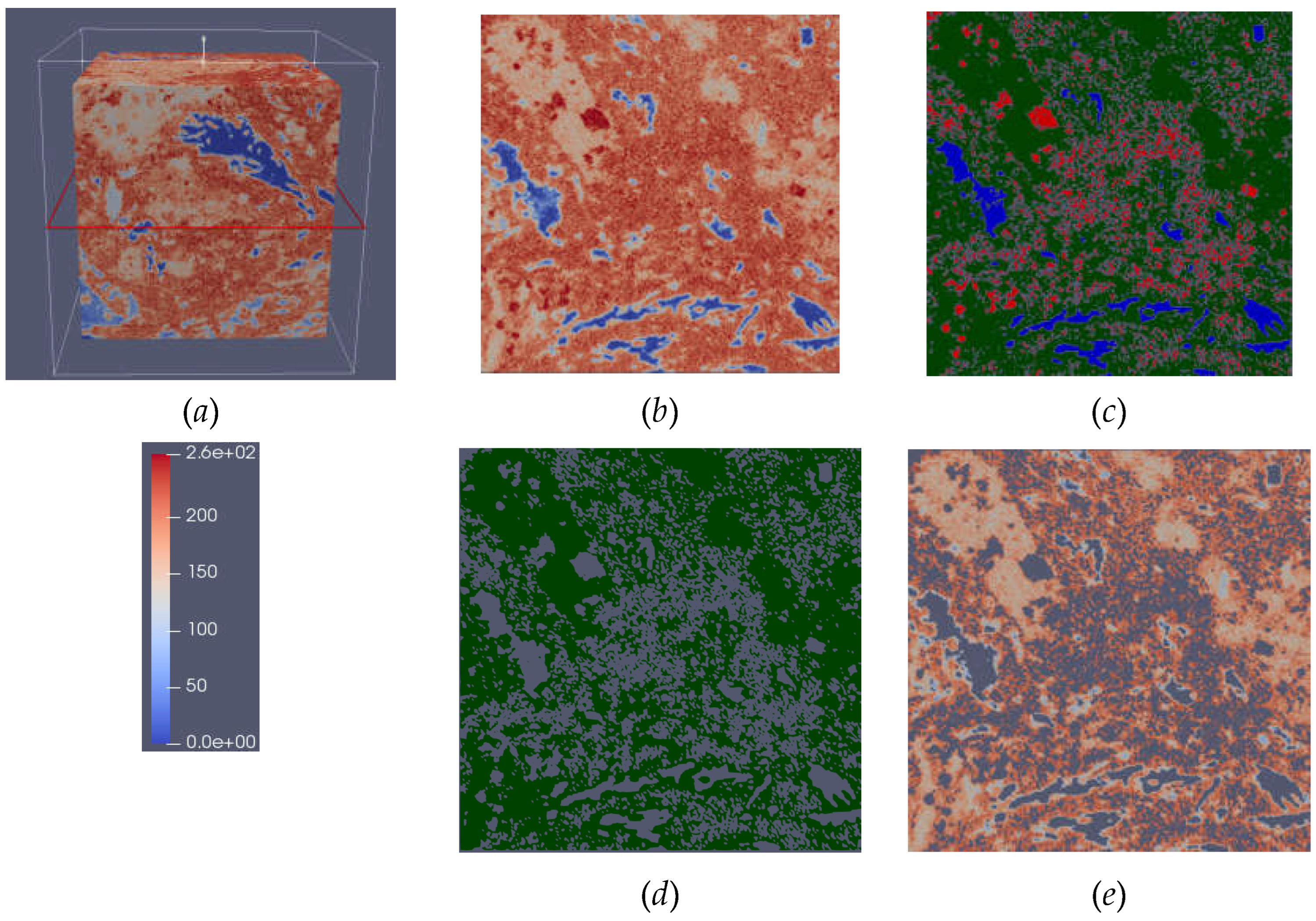
Figure 2.
The schematic of the 2D channel with separation and direction of the constant acceleration .
Figure 2.
The schematic of the 2D channel with separation and direction of the constant acceleration .
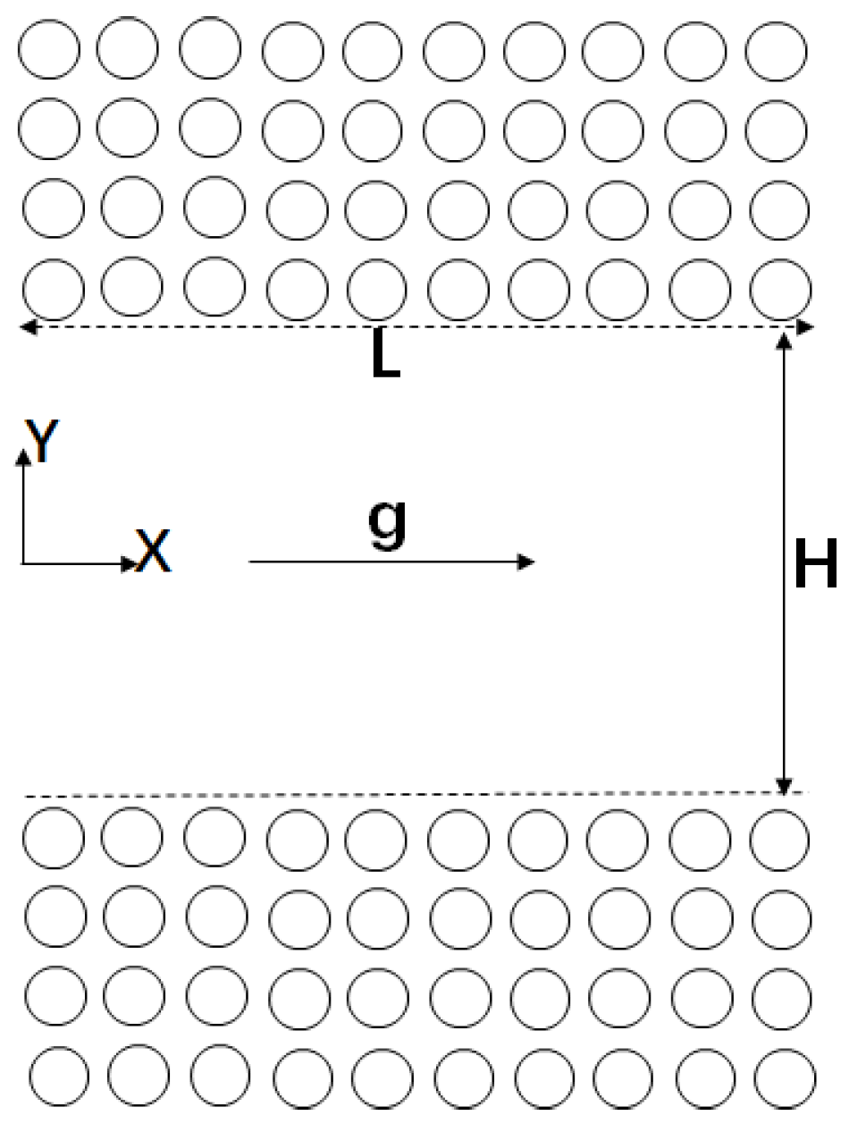
Figure 3.
Comparisons of the numerical solutions using two different integration schemes, respectively, with the corresponding exact solutions of the 2D channel flows with constant porosity and permeability.
Figure 3.
Comparisons of the numerical solutions using two different integration schemes, respectively, with the corresponding exact solutions of the 2D channel flows with constant porosity and permeability.
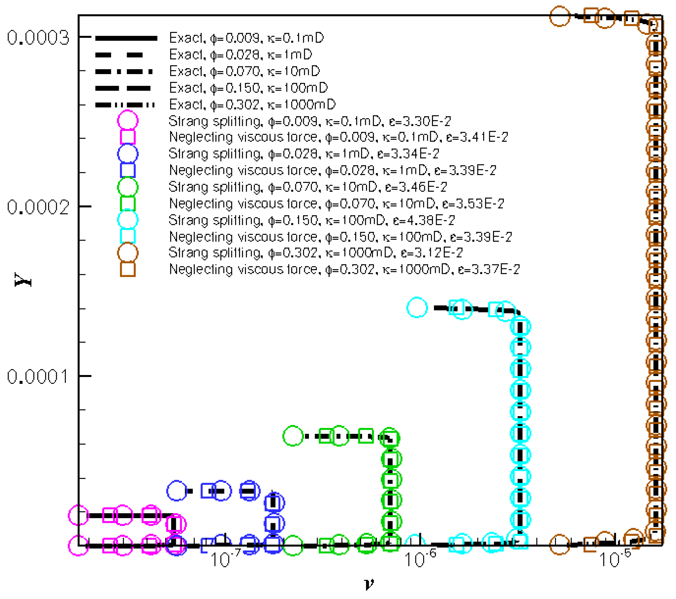
Figure 4.
Comparisons of the numerical solutions with the corresponding exact solutions of the 2D channel flows with constant porosity and permeability when the channel separation .
Figure 4.
Comparisons of the numerical solutions with the corresponding exact solutions of the 2D channel flows with constant porosity and permeability when the channel separation .
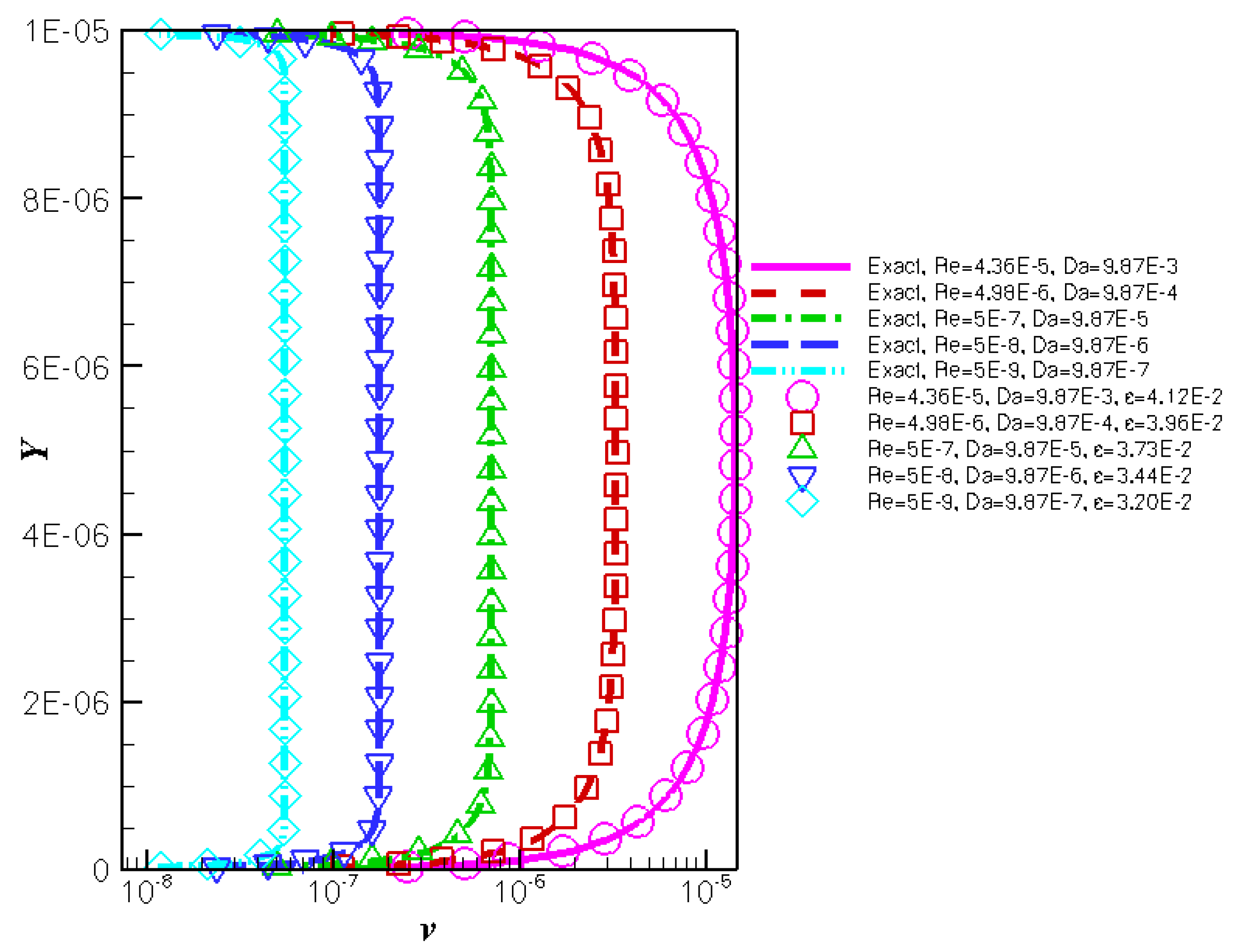
Figure 5.
Comparisons of the numerical solutions with the corresponding exact solutions of the 2D channel flows with constant porosity and permeability when the channel separation .
Figure 5.
Comparisons of the numerical solutions with the corresponding exact solutions of the 2D channel flows with constant porosity and permeability when the channel separation .
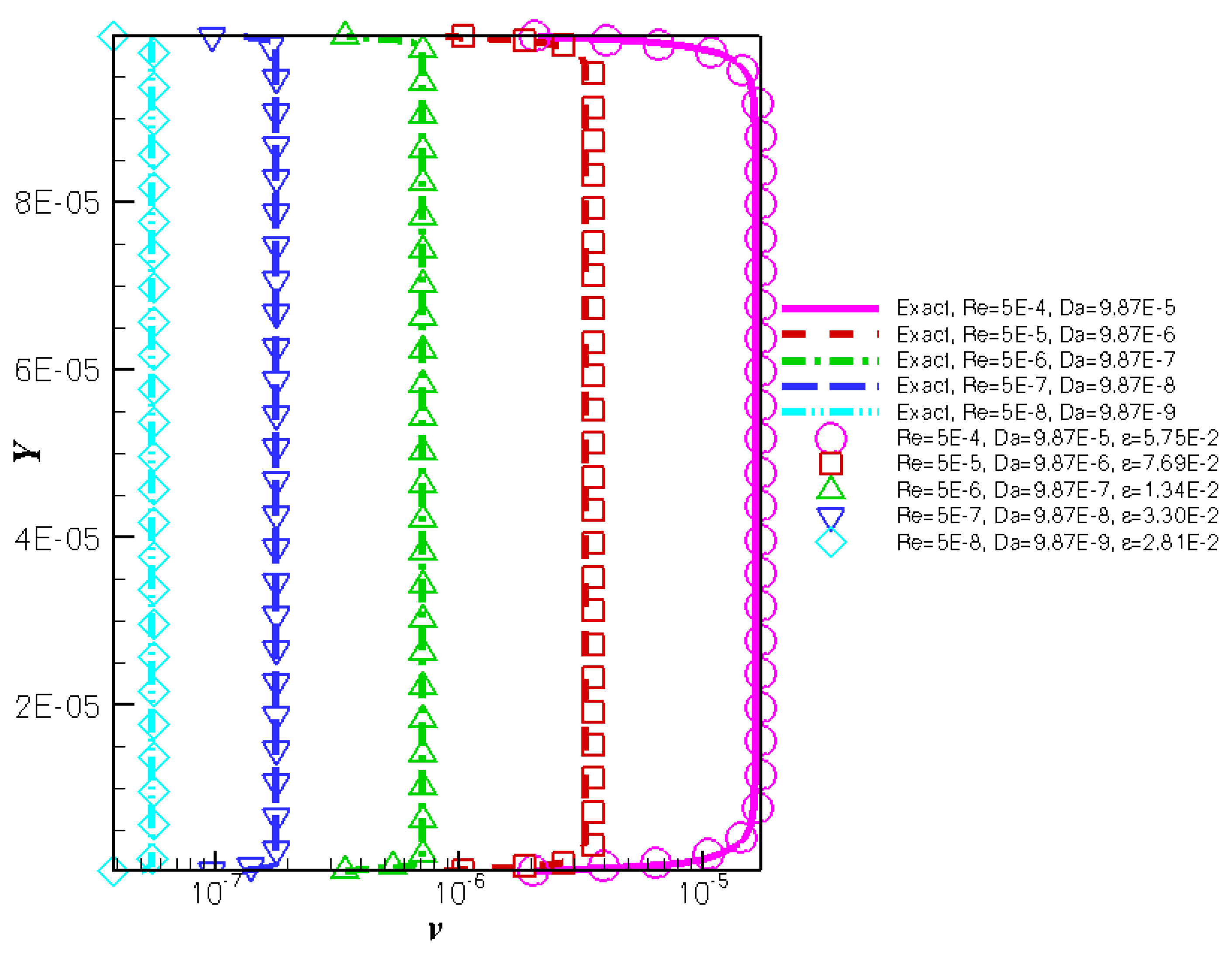
Figure 6.
Comparisons of the numerical solutions with the corresponding exact solutions of the 2D channel flows with constant porosity and permeability when the channel separation .
Figure 6.
Comparisons of the numerical solutions with the corresponding exact solutions of the 2D channel flows with constant porosity and permeability when the channel separation .
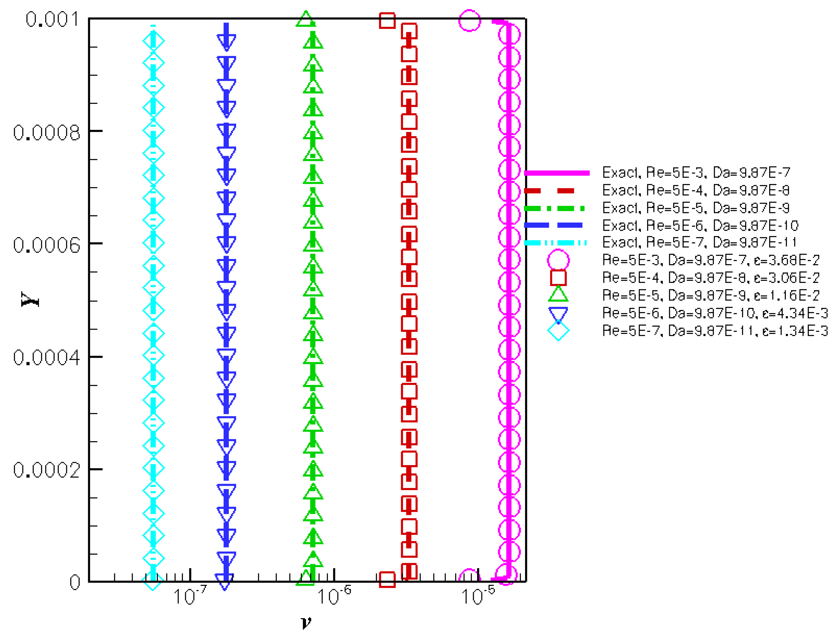
Figure 7.
Comparisons of the numerical solutions with the corresponding exact solutions of the 2D channel flows with constant porosity and permeability when the channel separation , during the time integration step the Strang splitting method is coercively applied.
Figure 7.
Comparisons of the numerical solutions with the corresponding exact solutions of the 2D channel flows with constant porosity and permeability when the channel separation , during the time integration step the Strang splitting method is coercively applied.
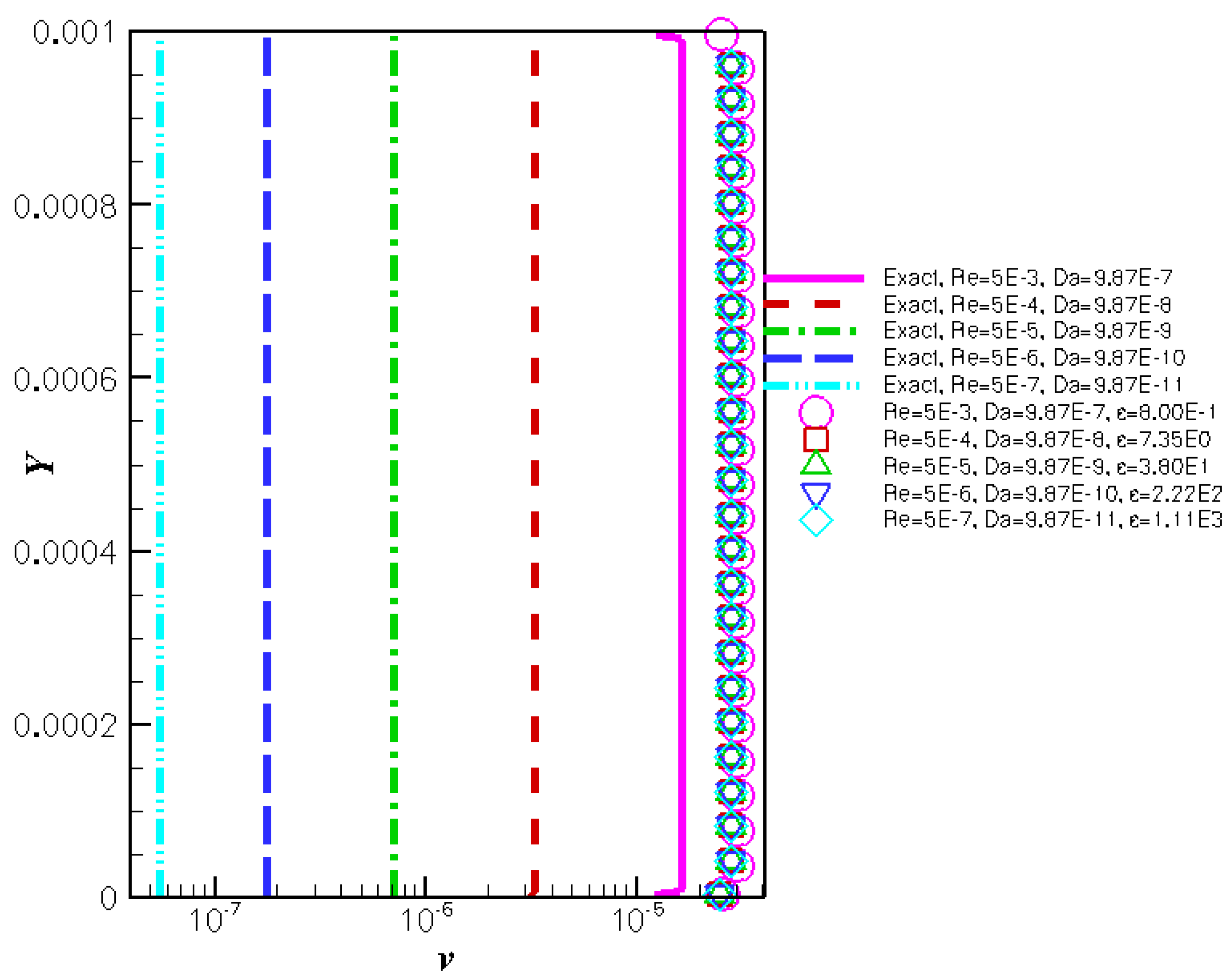
Figure 8.
Comparisons of the numerical solution for varying porosity 2D channel flow with the corresponding reference velocity at five observation lines, when .
Figure 8.
Comparisons of the numerical solution for varying porosity 2D channel flow with the corresponding reference velocity at five observation lines, when .
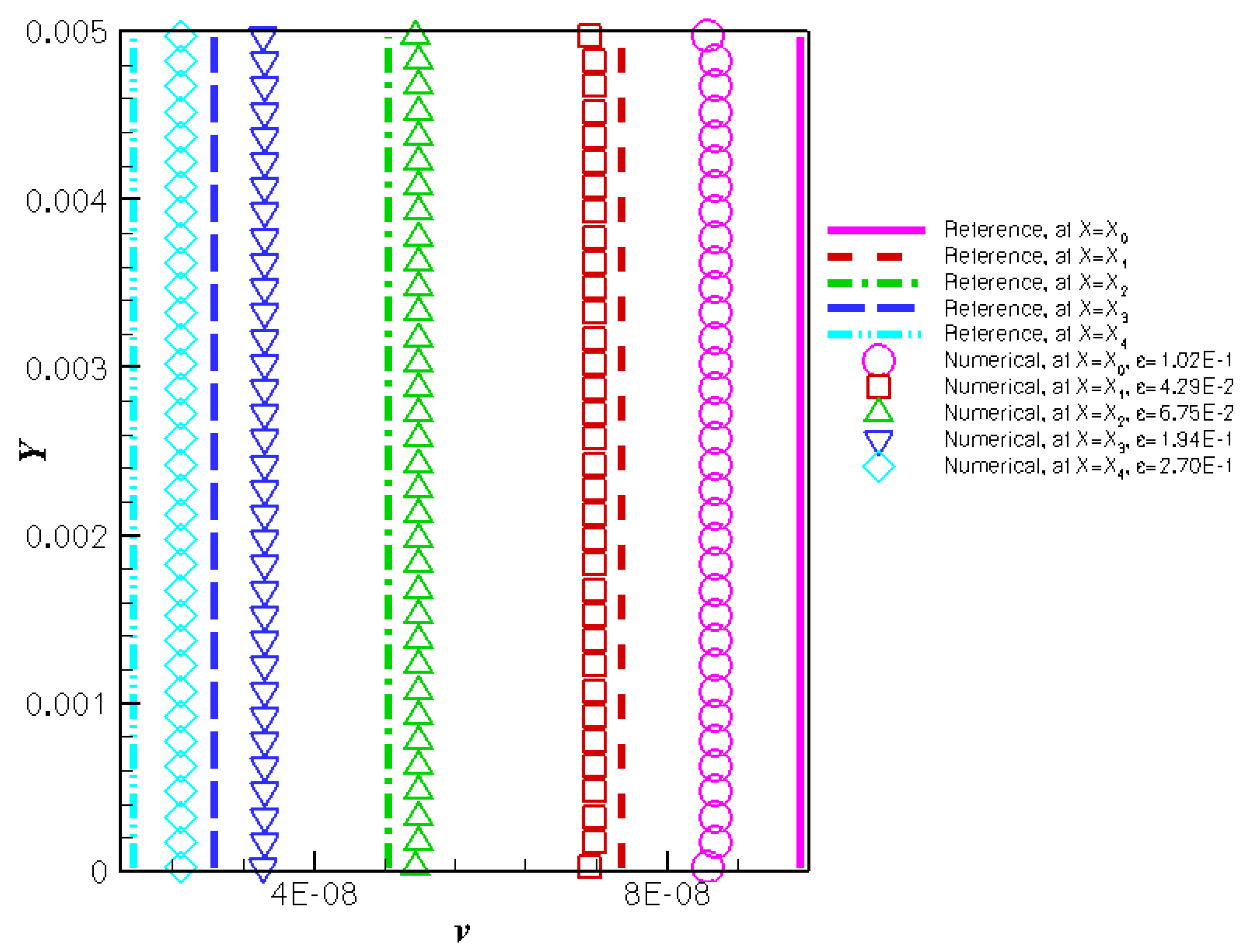
Figure 9.
Comparisons of the numerical solution for varying porosity 2D channel flow with the corresponding reference velocity at five observation lines, when and
Figure 9.
Comparisons of the numerical solution for varying porosity 2D channel flow with the corresponding reference velocity at five observation lines, when and
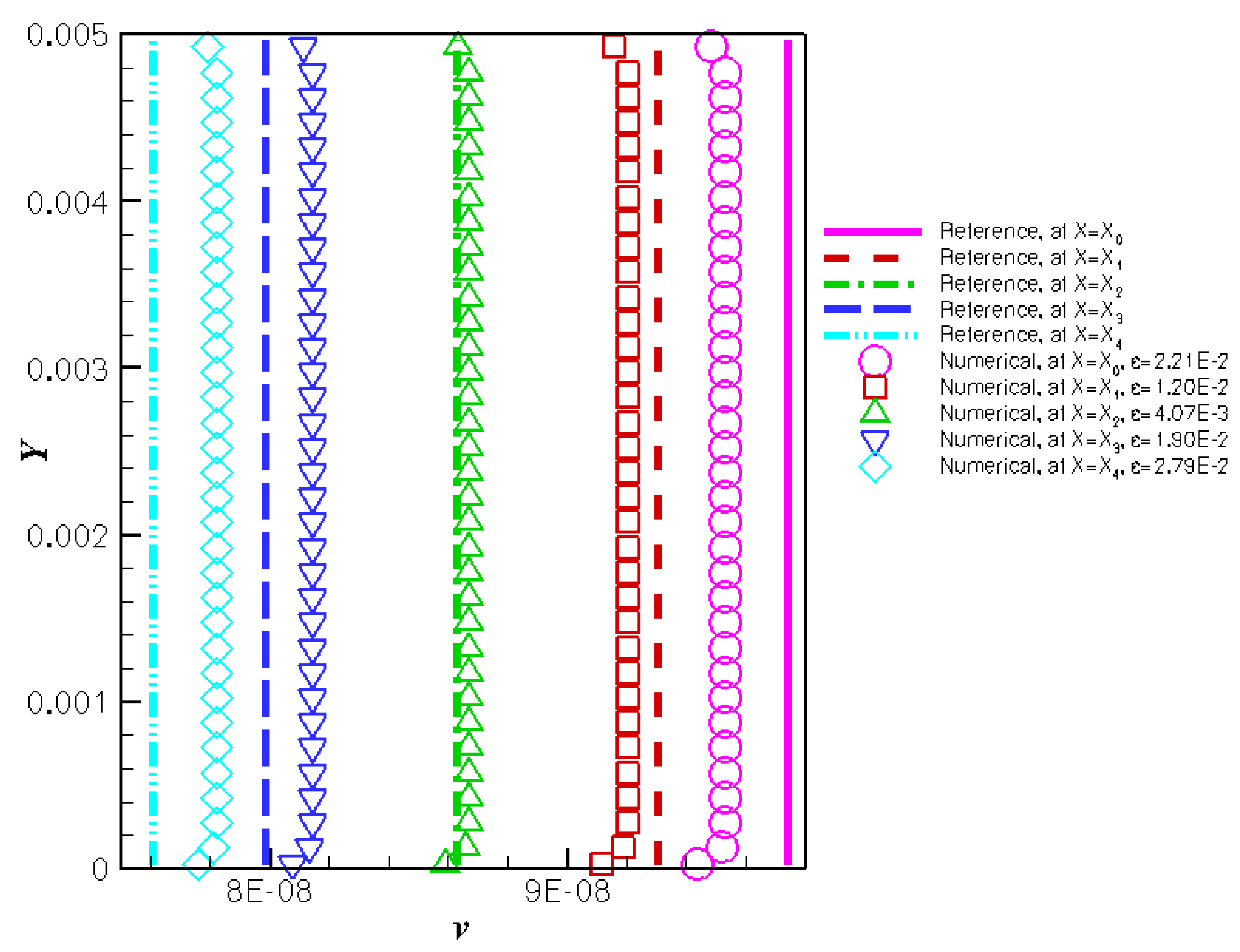
Figure 10.
Comparisons of the numerical solution for varying porosity 2D channel flow with the corresponding reference velocity at five observation lines, when and
Figure 10.
Comparisons of the numerical solution for varying porosity 2D channel flow with the corresponding reference velocity at five observation lines, when and
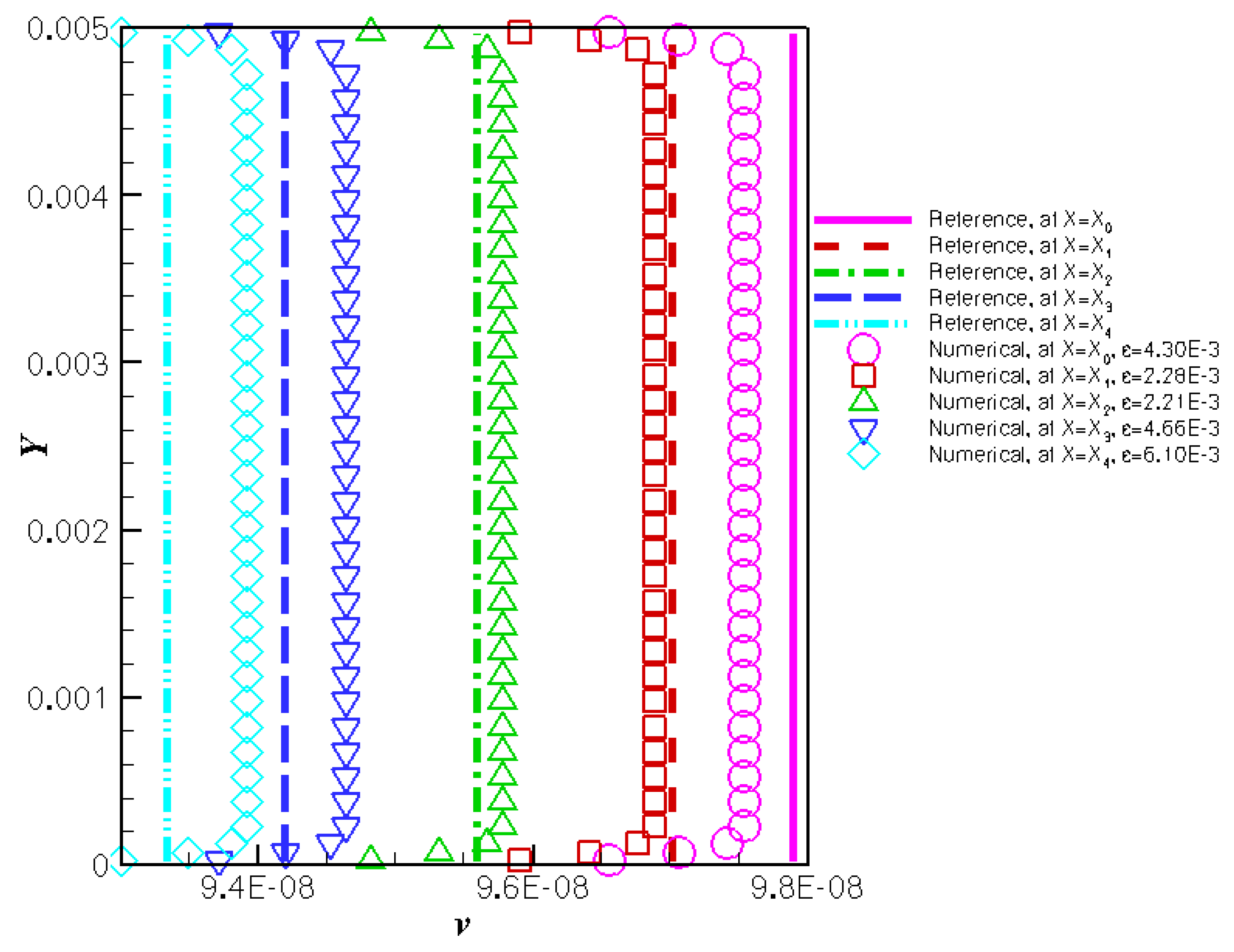
Figure 11.
Single cylinder in a periodic square lattice.
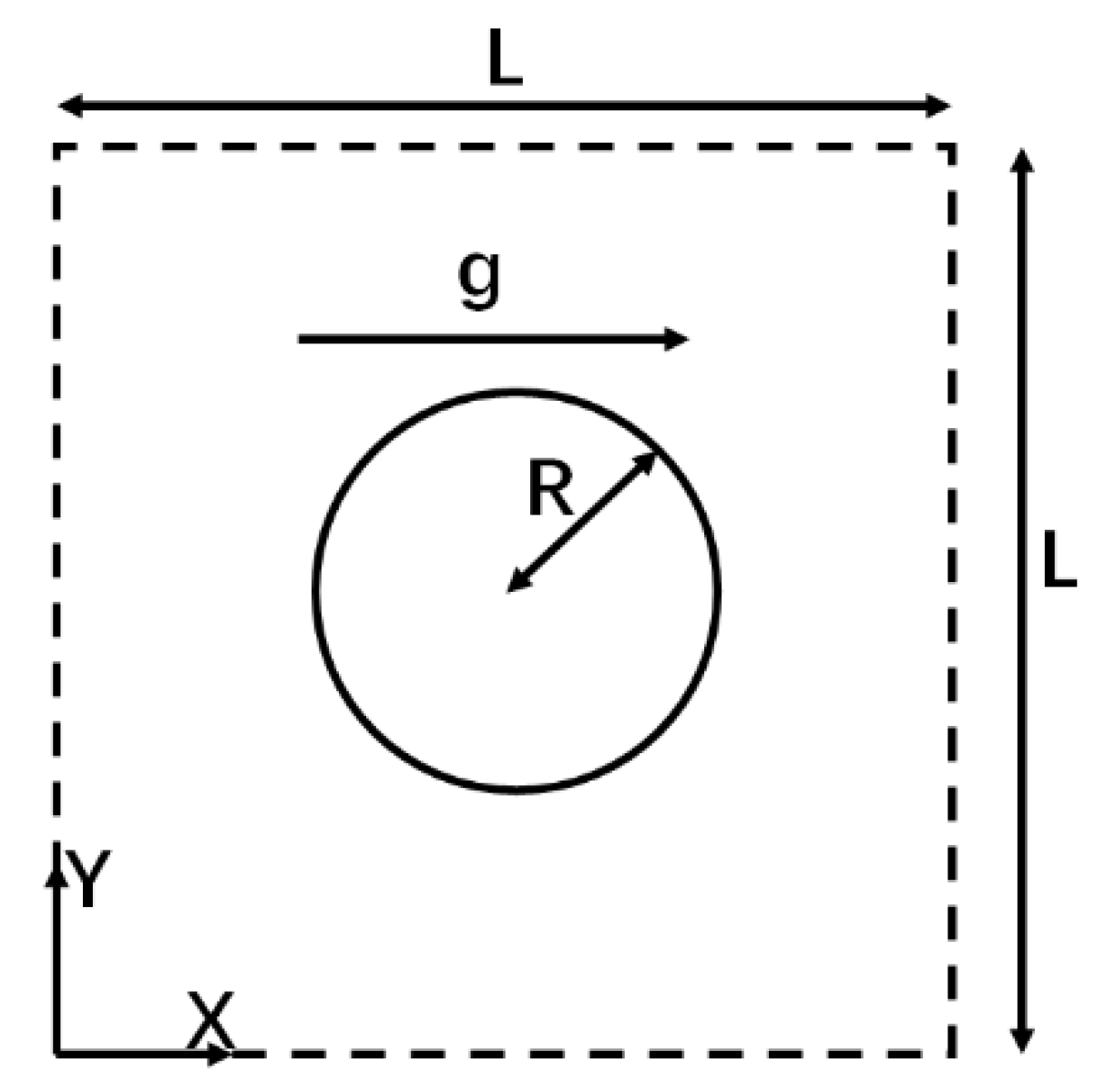
Figure 12.
Simulation result of the porous flow with over a pure solid cylinder (the white region): (a). The contour of X-component of velocity . (b). The contour of Y-component of velocity . (c). The pressure contour. (d). The velocity field (red) and streamlines (black).
Figure 12.
Simulation result of the porous flow with over a pure solid cylinder (the white region): (a). The contour of X-component of velocity . (b). The contour of Y-component of velocity . (c). The pressure contour. (d). The velocity field (red) and streamlines (black).
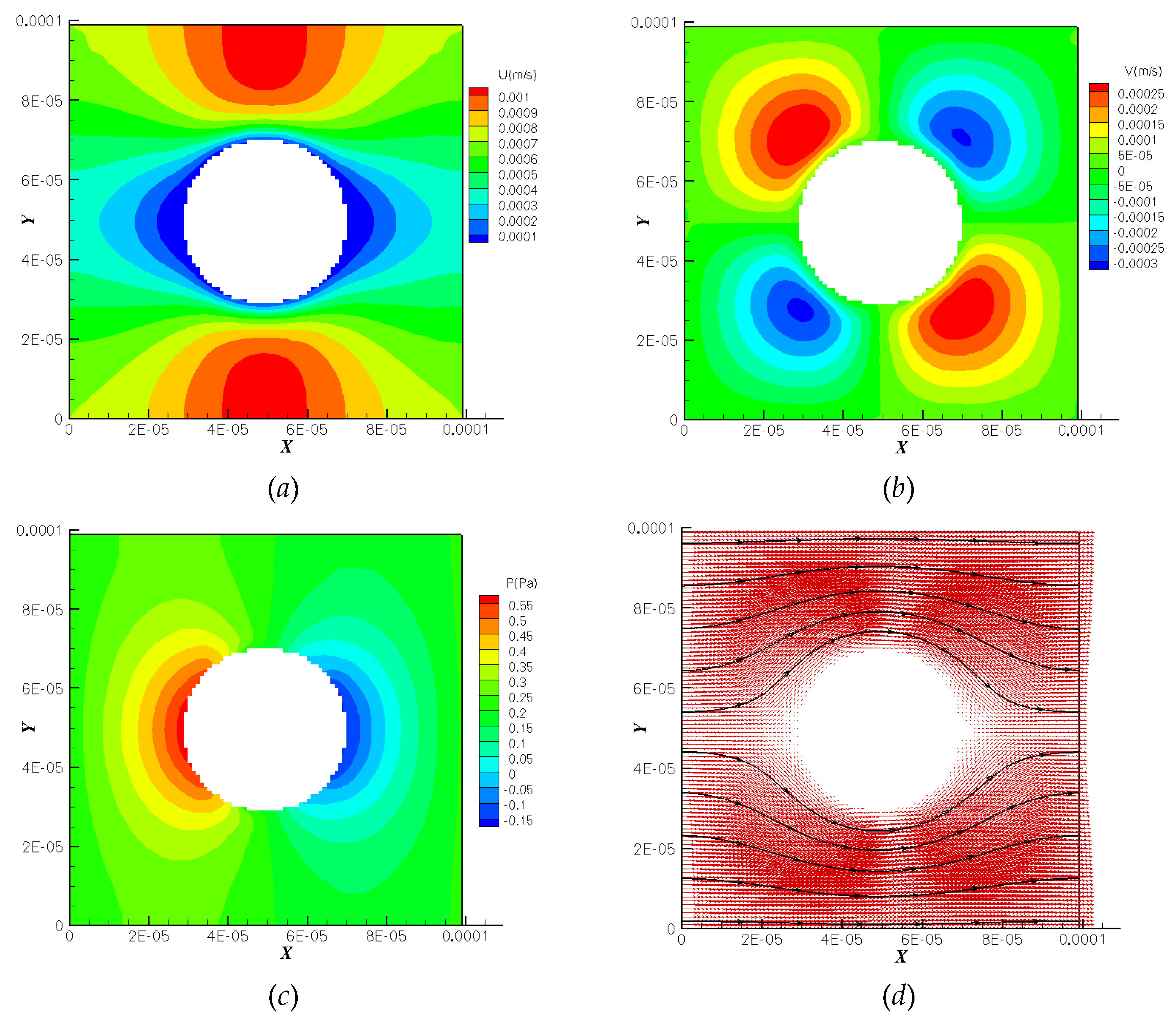
Figure 13.
Simulation result of the porous flow with over a pure solid cylinder (the white region): (a). The contour of X-component of velocity . (b). The contour of Y-component of velocity . (c). The pressure contour. (d). The velocity field (red) and streamlines (black).
Figure 13.
Simulation result of the porous flow with over a pure solid cylinder (the white region): (a). The contour of X-component of velocity . (b). The contour of Y-component of velocity . (c). The pressure contour. (d). The velocity field (red) and streamlines (black).
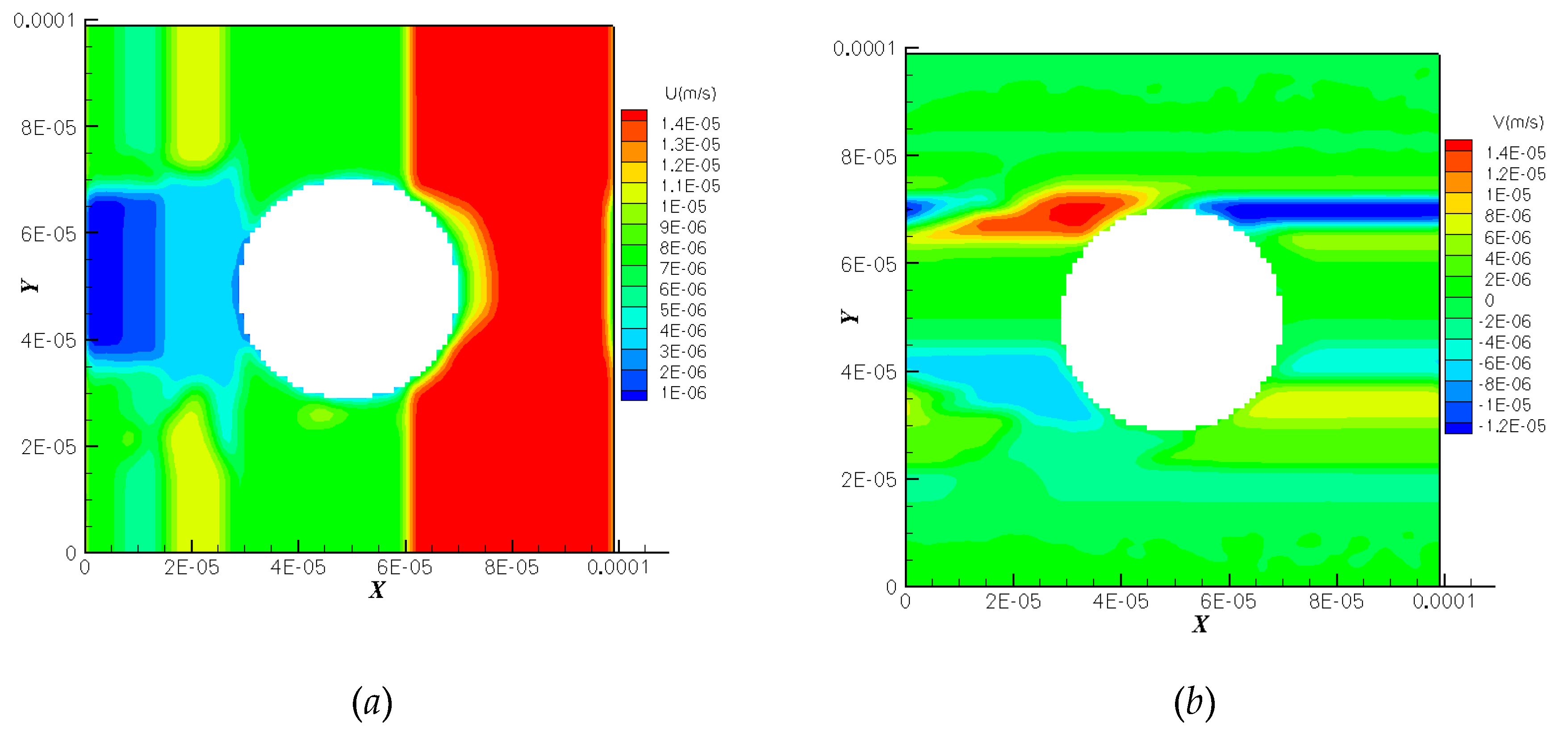
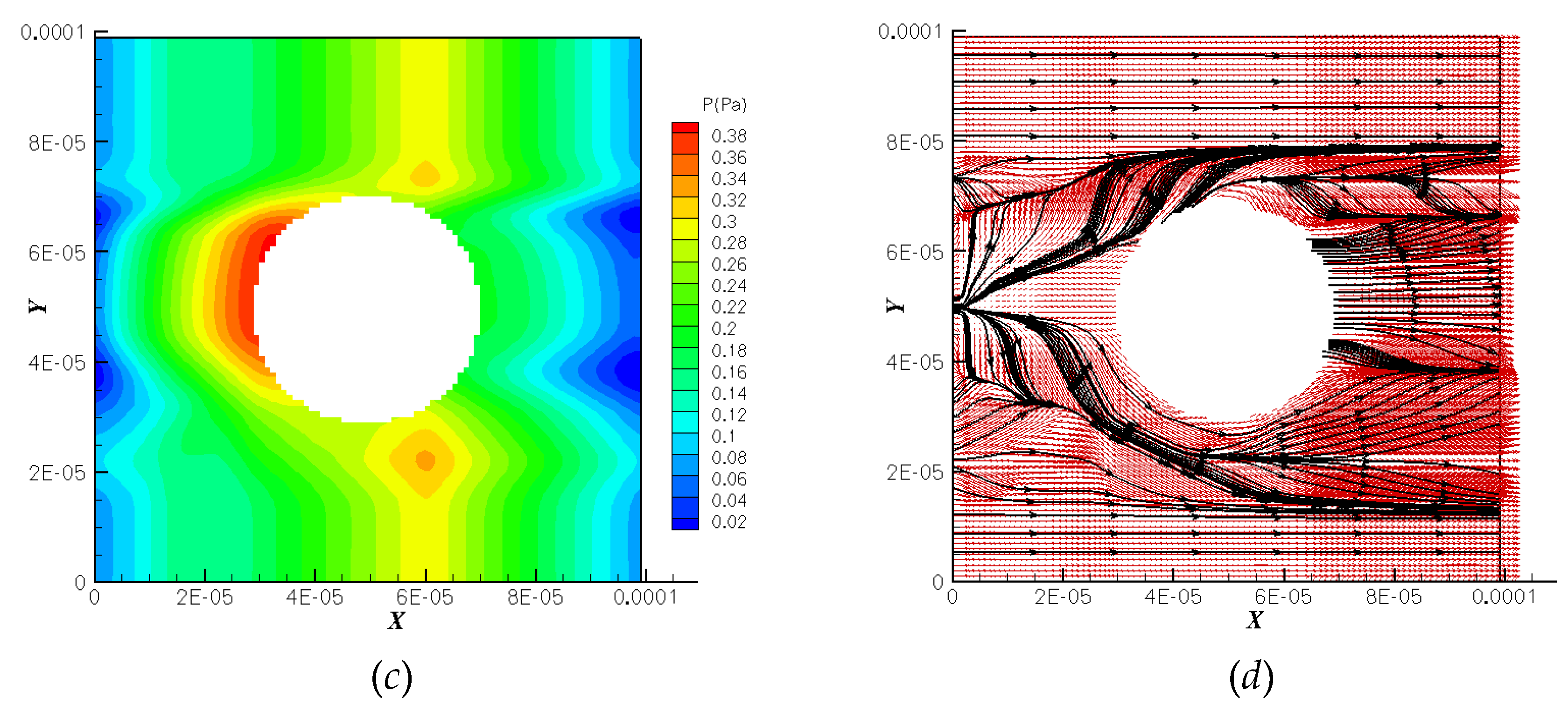
Figure 14.
Simulation result of the porous flow with over a gradually denser cylinder (within the pink dashed line) where the porosity decreases from at the edge to at the center: (a). The contour of X-component of velocity . (b). The contour of Y-component of velocity . (c). The pressure contour. (d). The velocity field (red) and streamlines (black).
Figure 14.
Simulation result of the porous flow with over a gradually denser cylinder (within the pink dashed line) where the porosity decreases from at the edge to at the center: (a). The contour of X-component of velocity . (b). The contour of Y-component of velocity . (c). The pressure contour. (d). The velocity field (red) and streamlines (black).
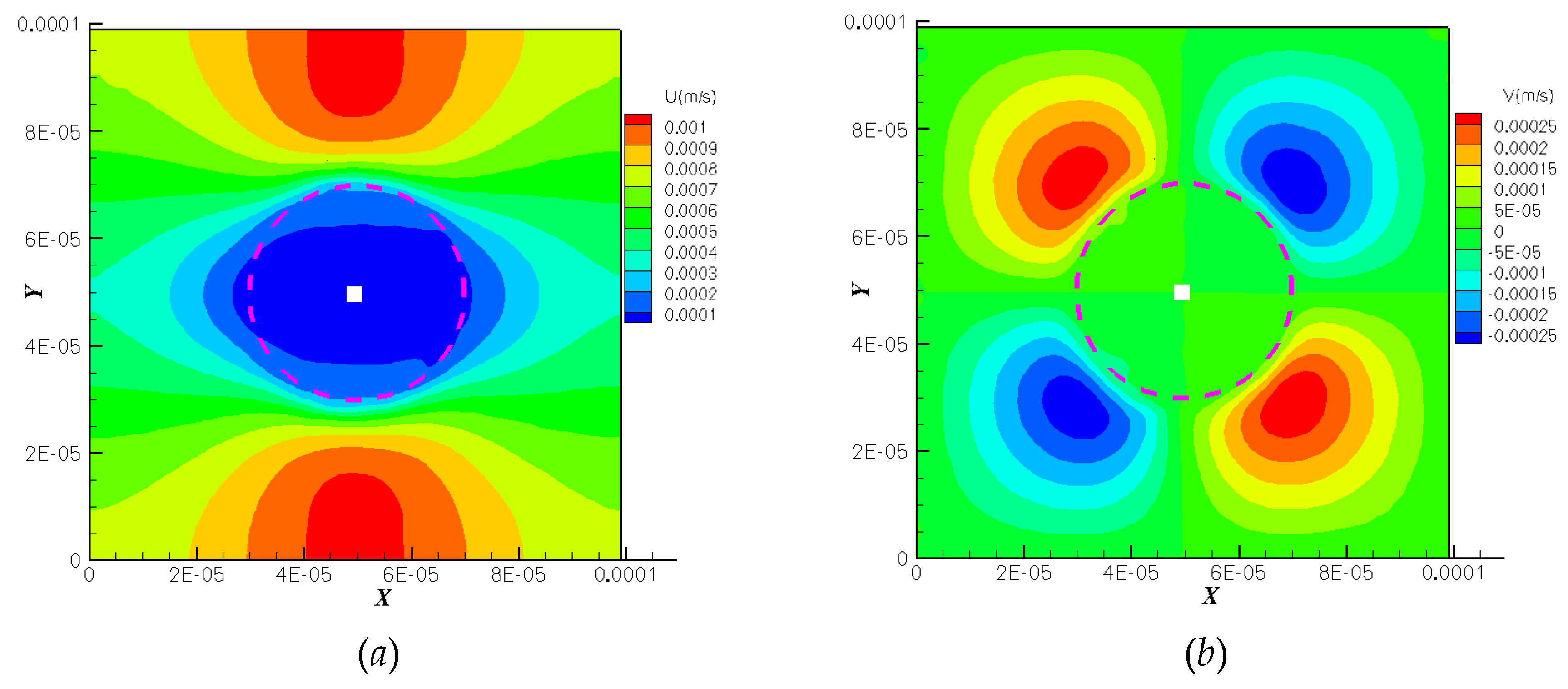
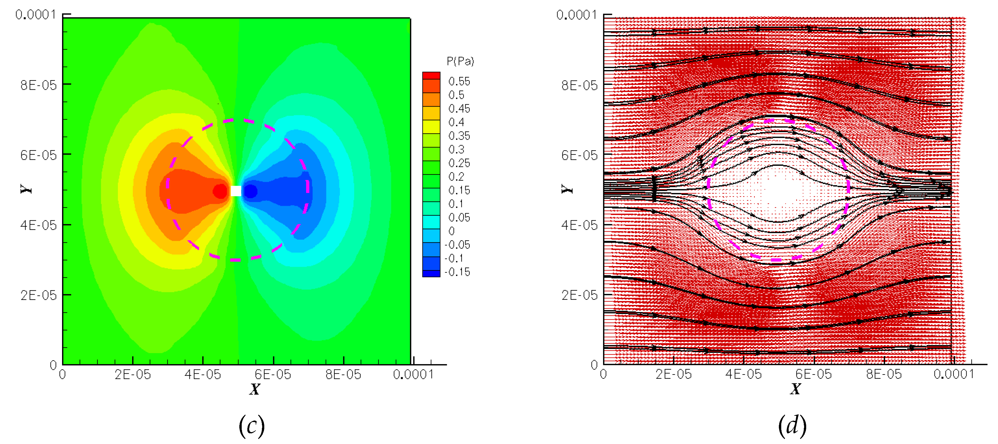
Figure 15.
Simulation result of the porous flow with over a gradually looser cylinder (within the pink dashed line) where the porosity increases from at the edge to at the center: (a). The contour of X-component of velocity . (b). The contour of Y-component of velocity . (c). The pressure contour. (d). The velocity field (red) and streamlines (black).
Figure 15.
Simulation result of the porous flow with over a gradually looser cylinder (within the pink dashed line) where the porosity increases from at the edge to at the center: (a). The contour of X-component of velocity . (b). The contour of Y-component of velocity . (c). The pressure contour. (d). The velocity field (red) and streamlines (black).
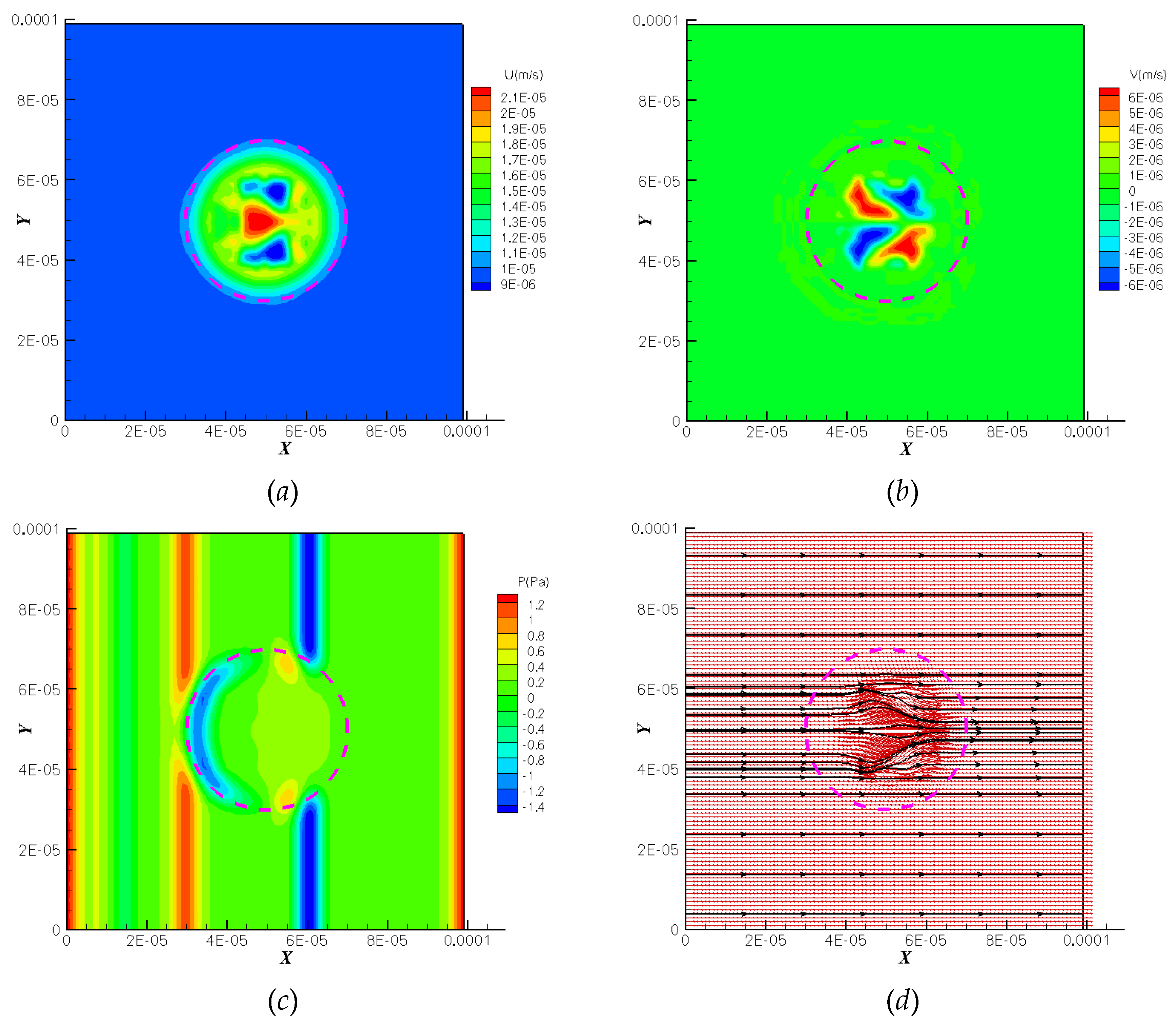
Figure 16.
Simulation result of the flow through a 2D digital core: (a). The contour of X-component of velocity . (b). The pressure contour. (c). The porosity contour.
Figure 16.
Simulation result of the flow through a 2D digital core: (a). The contour of X-component of velocity . (b). The pressure contour. (c). The porosity contour.
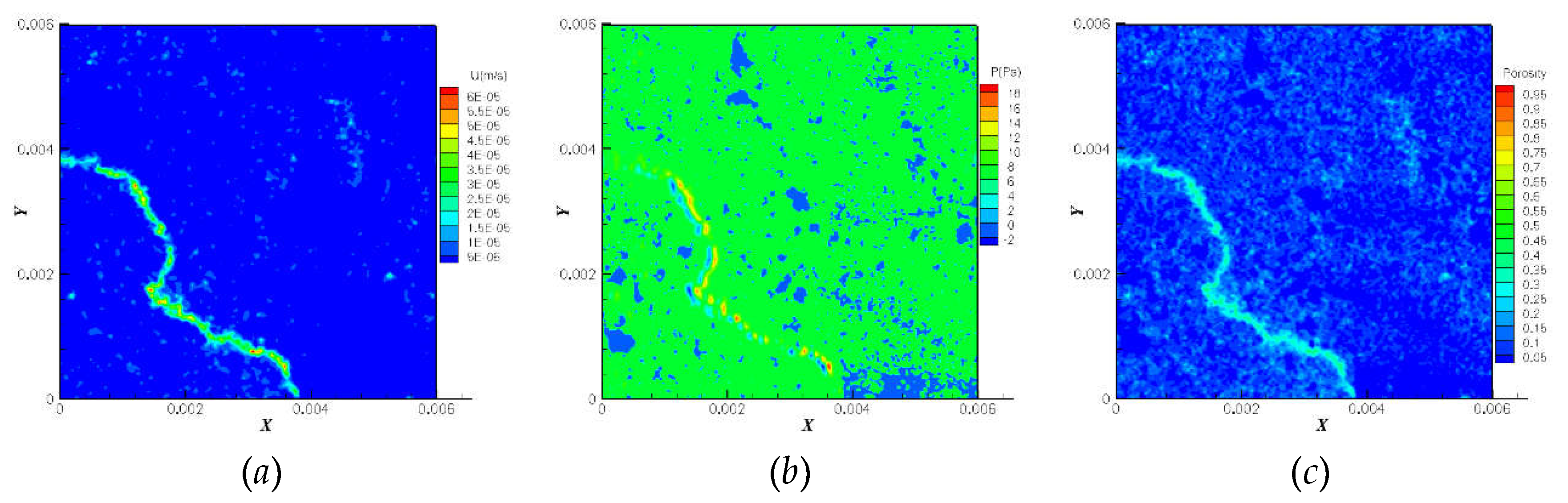
Figure 17.
Simulation result of the flow through a 3D digital core: (a). The contour of Z-component of velocity (values of are displayed). (b). The pressure contour (values of and are displayed). (c). The porosity contour (values of are displayed).
Figure 17.
Simulation result of the flow through a 3D digital core: (a). The contour of Z-component of velocity (values of are displayed). (b). The pressure contour (values of and are displayed). (c). The porosity contour (values of are displayed).
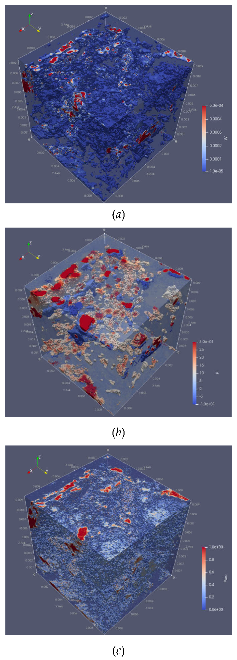

Table 1.
The porosity-permeability pairs of the channel and the critical resolutions when , and the RMSEP by using two different integration schemes, respectively.
Table 1.
The porosity-permeability pairs of the channel and the critical resolutions when , and the RMSEP by using two different integration schemes, respectively.
| m | m | m | m | m | |
Table 2.
The porosity-permeability pairs of the channel and the Reynolds number and Darcy number of the flows and the RMSEP of the numerical solution when .
Table 2.
The porosity-permeability pairs of the channel and the Reynolds number and Darcy number of the flows and the RMSEP of the numerical solution when .
| Re | |||||
| Da | |||||
Table 3.
The porosity-permeability pairs of the channel and the Reynolds number and Darcy number of the flows and the RMSEP of the numerical solution when.
Table 3.
The porosity-permeability pairs of the channel and the Reynolds number and Darcy number of the flows and the RMSEP of the numerical solution when.
| Re | |||||
| Da | |||||
Table 4.
The porosity-permeability pairs of the channel and the Reynolds number and Darcy number of the flows and the RMSEP of the numerical solution when .
Table 4.
The porosity-permeability pairs of the channel and the Reynolds number and Darcy number of the flows and the RMSEP of the numerical solution when .
| Re | |||||
| Da | |||||
Disclaimer/Publisher’s Note: The statements, opinions and data contained in all publications are solely those of the individual author(s) and contributor(s) and not of MDPI and/or the editor(s). MDPI and/or the editor(s) disclaim responsibility for any injury to people or property resulting from any ideas, methods, instructions or products referred to in the content. |
© 2026 by the authors. Licensee MDPI, Basel, Switzerland. This article is an open access article distributed under the terms and conditions of the Creative Commons Attribution (CC BY) license (http://creativecommons.org/licenses/by/4.0/).
Copyright: This open access article is published under a Creative Commons CC BY 4.0 license, which permit the free download, distribution, and reuse, provided that the author and preprint are cited in any reuse.