
Submitted:
22 September 2026
Posted:
23 September 2026
You are already at the latest version
Abstract
Sensor failures, communication interruptions, and other monitoring problems can lead to missing acceleration responses in structural health monitoring of offshore platforms. To address this issue, a hierarchical feature fusion reconstruction (HFFR) method is proposed. The method employs multi-scale local morphology encoding to characterize local response morphology over different temporal neighborhoods, uses bidirectional temporal modeling to capture response evolution before and after the missing data, and adaptively weights temporal information according to feature correlation. A dataset is constructed using numerical simulation data from an offshore platform under different wave–current conditions, and the proposed method is evaluated through ablation and comparative experiments. After introducing multi-scale local morphology encoding and adaptive feature weighting into the bidirectional temporal modeling framework, the RMSE decreases from 0.5036 to 0.1109, while R² increases from 0.7581 to 0.9883, confirming the effectiveness of the hierarchical information representation framework. The results show that HFFR can recover the major peaks and valleys, amplitude envelopes, and local fluctuations of the missing responses, thereby improving both reconstruction accuracy and the preservation of dynamic response characteristics. The current validation is mainly based on high-fidelity numerical simulations; therefore, the applicability of the proposed method in real monitoring environments should be further verified through physical model tests.
Keywords:
offshore platform
; structural health monitoring
; time series
; acceleration response
; missing data reconstruction
; hierarchical feature fusion
; deep learning
1. Introduction
Offshore platforms are continuously exposed to complex environmental loads induced by wind, waves, and currents throughout their service life. Their structural performance may also gradually deteriorate due to seawater corrosion, material aging, and accumulated fatigue damage. Structural health monitoring (SHM) systems provide essential data for modal parameter identification, structural condition assessment, damage diagnosis, and remaining service life prediction by continuously collecting structural responses such as acceleration, strain, and displacement[1,2]. For large offshore structures, sensor deployment is generally limited to a number of critical locations because of installation constraints, deployment costs, and maintenance difficulties. Therefore, long-term monitoring data collected at each measurement location are of considerable value[3,4]. However, sensor failures, power supply abnormalities, communication interruptions, and data transmission errors are difficult to completely avoid in complex marine environments and may result in continuous loss of monitoring data[5]. Missing data can disrupt the integrity and continuity of structural response time histories and may consequently reduce the reliability of subsequent modal identification, condition assessment, and damage diagnosis. Accurate reconstruction of missing structural responses is therefore important for maintaining the quality of SHM data from offshore platforms[6].
Existing methods for reconstructing missing structural responses can generally be divided into physics-based and data-driven approaches. Physics-based methods establish relationships between unknown and measured responses using prior knowledge such as structural dynamic equations, finite element models, modal parameters, or external loads. Structural responses have been reconstructed using approaches such as modal superposition, finite element model updating, and load identification[7,8,9]. These methods have relatively clear physical interpretations, but their performance depends strongly on the accuracy of the structural model, boundary conditions, and loading information. For large structures operating for long periods in complex marine environments, both structural parameters and environmental loads involve uncertainties. Consequently, constructing and continuously updating a high-fidelity reference model remains challenging.
In contrast, data-driven methods recover missing data directly from the statistical correlations and temporal dependencies contained in historical monitoring responses, without requiring accurate external loading information or a high-fidelity finite element model. Representative approaches include Kalman filtering[10,11,12], Bayesian inference[13,14,15,16], and compressed sensing[17,18,19,20]. These methods can achieve satisfactory reconstruction under appropriate conditions. However, they generally rely on specific assumptions regarding state-space models, probability distributions, or signal sparsity[21], which may limit their ability to represent nonlinear relationships in complex and nonstationary structural responses.
In recent years, deep learning has provided new approaches for recovering missing data in structural monitoring[22,23]. Fan et al.[24] employed a convolutional neural network to learn the mapping between incomplete and complete acceleration responses. Oh et al.[25] used a CNN to recover structural responses under data-loss conditions. Pan et al.[26] combined long short-term memory (LSTM) networks with correlations among sensors to recover structural monitoring data. Lu et al.[27] employed a bidirectional long short-term memory (BiLSTM) network to extract temporal information in both directions from acceleration responses, thereby improving the reconstruction of long-term structural responses. Wang et al.[28] introduced an attention mechanism into a BiLSTM network to improve acceleration response reconstruction by adjusting the contributions of features at all timesteps.
Despite the progress achieved by deep learning methods in recovering missing structural monitoring data, effective reconstruction still requires the coordinated use of local dynamic information and temporal relationships. First, structural acceleration responses exhibit different local response morphology over different temporal neighborhoods, and features extracted at a single scale may not adequately represent both rapid oscillations and slowly varying response patterns. Second, no valid observations are available within continuously missing data, making it necessary to exploit the available responses before and after the missing data as well as the temporal evolution of the structural response. In addition, temporal features at different timesteps have diverse degrees of correlation with the response to be reconstructed. How to identify and strengthen the temporal information that is more closely related to response reconstruction therefore remains an important issue for improving reconstruction performance.
To address these issues, a hierarchical feature fusion reconstruction (HFFR) method is proposed for reconstructing missing acceleration responses of offshore platforms. Rather than directly learning a single mapping from the original time series, HFFR organizes structural response information at three levels: local response morphology, temporal evolution, and feature correlation. Local response morphology is characterized using response information from different temporal neighborhoods. Bidirectional temporal modeling is then used to learn response evolution from the available observations before and after the missing data, while the contributions of temporal features are adaptively adjusted according to feature correlation. In this way, the proposed method reconstructs missing acceleration responses through hierarchical information representation. A missing-data dataset is constructed from numerical responses of a jacket offshore platform under multiple wave–current conditions, and the reconstruction performance of HFFR is evaluated through ablation studies and comparisons with baseline models.
The remainder of this paper is organized as follows. Section 2 presents the basic principles and overall framework of HFFR, including multi-scale local response morphology encoding, bidirectional temporal modeling, and correlation-based adaptive feature weighting. Section 3 describes the numerical model of the offshore platform, dataset construction, data preprocessing, and model training settings. Section 4 presents the ablation study and reconstruction results obtained using different models, followed by an analysis and discussion of their performance. Finally, Section 5 summarizes the main conclusions, discusses the limitations of the current study, and outlines directions for future research.
2. Materials and Methods
The proposed hierarchical feature fusion reconstruction method considers three complementary aspects of structural response information: local morphological characteristics, temporal evolution, and differences in the importance of temporal information. Accordingly, multi-scale local response morphology encoding, bidirectional temporal modeling, and correlation-based adaptive feature weighting are employed to characterize these different aspects.
2.1. Multi-Scale Local Response Morphology Encoding
Structural acceleration responses exhibit pronounced local oscillatory characteristics, and temporal neighborhoods of different widths reflect response morphology at different scales. Within a relatively narrow temporal neighborhood, the response is mainly characterized by peak-to-valley transitions, rapid amplitude variations, and local oscillations. In a wider temporal neighborhood, local amplitude envelopes, slowly varying waveforms, and local periodic variations can be observed. Feature extraction with a fixed receptive field is therefore difficult to simultaneously represent information at these different scales.
To address this issue, multi-scale local response morphology encoding is employed to characterize structural acceleration responses in parallel over multiple temporal receptive fields. Smaller receptive fields are more sensitive to rapid variations between adjacent timesteps, whereas larger receptive fields facilitate the aggregation of slowly varying information over wider local neighborhoods. The features obtained at different scales are then concatenated along the channel dimension to form a multi-scale feature sequence containing complementary local response morphology information.
2.2. Bidirectional Temporal Modeling
Structural acceleration responses exhibit clear temporal dependencies among different timesteps. Relying only on local information is insufficient for complete recovery of missing data, and the response evolution over a longer temporal range should therefore be considered. LSTM networks use cell states and gating mechanisms to adaptively control the retention, forgetting, and updating of historical information, thereby improving the modeling of both short- and long-term temporal dependencies.
However, unidirectional prediction based only on the responses preceding the missing data cannot fully exploit all available temporal information and may lead to increasing prediction errors as the amount of missing data increases. Therefore, a bidirectional long short-term memory (BiLSTM) network is employed to model bidirectional temporal dependencies in the structural dynamic response, allowing the available responses both before and after the missing data to contribute to the reconstruction process.
2.3. Correlation-Based Adaptive Feature Weighting
During missing-response reconstruction, information at various timesteps does not contribute equally to the recovery of the target response. Temporal features with stronger correlation to the dynamic state of the target response generally provide more useful information, whereas weakly correlated features may introduce redundancy and interfere with reconstruction. Therefore, temporal dependency modeling alone is insufficient to distinguish the different contributions of temporal features to the reconstruction result.
A correlation-based adaptive feature weighting mechanism is employed to fuse temporal features from different timesteps. The mechanism quantifies feature correlation across all timesteps and adaptively adjusts their contributions to the fused representation, allowing information more strongly correlated with the target response to receive greater weight.
2.4. Hierarchical Feature Fusion and Overall Framework
Based on the three information representation mechanisms described above, a hierarchical feature fusion reconstruction method is developed for missing acceleration responses. The overall framework is shown in Figure 1.
First, the input response sequence of length is processed using multi-scale local response morphology encoding. The feature representation obtained from the m-th convolutional branch is expressed as follows:
(1)
and the features extracted at different scales are concatenated along the channel dimension:
(2)
where denotes the number of convolutional branches, and are the weight parameters and bias of the m-th convolutional branch, respectively, and denotes the nonlinear activation function.
The multi-scale local features are subsequently processed using long short-term memory networks to model temporal dependencies. For the input feature at timestep , the LSTM controls the retention and updating of historical information through the input, forget, and output gates. The calculation can be expressed as follow:
(3)
where , , and denote the input, forget, and output gates, respectively; is the candidate cell state; and are the cell and hidden states, respectively; and denote the sigmoid and hyperbolic tangent activation functions; and represents element-wise multiplication.
To simultaneously use the available responses before and after the missing data, a BiLSTM is further employed to update the hidden states in the forward and backward temporal directions:
(4)
(5)
The hidden states from the two directions are then combined as follows:
(6)
The bidirectional temporal feature matrix over all timesteps is therefore obtained as follows:
(7)
To further distinguish the contributions of temporal features at different timesteps to the reconstruction process, the bidirectional temporal feature matrix is projected into the query matrix , key matrix , and value matrix using learnable transformation matrices:
(8)
Feature correlation among different timesteps is obtained from the scaled dot product of Q and K, and the resulting values are normalized using the SoftMax function to obtain the attention weights:
(9)
where WQ, WK, and WV denote the learnable transformation matrices for the query, key, and value, respectively, and dk is the dimension of the key vector.
The value matrix V is then weighted using A to obtain the weighted feature representation:
(10)
The weighted temporal features are transformed through a linear mapping followed by a Gaussian Error Linear Unit (GELU) activation function, and the reconstructed response is finally obtained through the output layer:
(11)
(12)
where and are the weight matrix and bias of the linear mapping layer, respectively; denotes the Gaussian Error Linear Unit activation function; and are the weight matrix and bias of the output layer, respectively.
3. Numerical Dataset Generation and Experimental Setup
To evaluate the capability of the proposed hierarchical feature fusion reconstruction method to recover missing acceleration responses of offshore platforms, complete acceleration responses under different wave–current conditions were first obtained using a finite element model of a jacket offshore platform. A missing-response dataset was then constructed based on these complete responses. The original data were subsequently partitioned, standardized, and segmented using sliding windows to generate sequence samples for model training, validation, and testing.
3.1. Numerical Simulation of the Offshore Platform
All numerical simulations in this study were performed using ANSYS 2022 R1. The jacket offshore platform has an overall height of 65 m, a deck length of 30 m, a deck width of 20 m, and an operating water depth of 45 m. The structural material has a density of 7850 kg/ m³, an elastic modulus of 205 GPa, and a Poisson’s ratio of 0.3. PIPE288 elements were used for the platform legs and supporting members, PIPE20 elements for the legs below the mudline, BEAM4 elements for the upper-platform beam system, and SHELL43 elements for the deck. Fixed boundary conditions were applied at the bottoms of the four platform legs to simplify the pile–soil interaction. Rayleigh damping was adopted in the dynamic analysis, with the mass-proportional and stiffness-proportional damping coefficients set to α=0.1575 and β=2.5389×10⁻³, respectively.
Considering sensor installation conditions and maintenance accessibility, acceleration monitoring points were arranged on both the lower and upper decks of the platform. Each deck was divided into six regions, with one monitoring point placed in each region, resulting in a total of 12 acceleration monitoring points. Monitoring points 1–6 were located on the lower deck, whereas monitoring points 7–12 were located on the upper deck. The finite element model and monitoring-point layout are shown in Figure 2.
To obtain structural dynamic responses under different sea states, environmental loads induced by the combined effects of random waves and currents were considered. Random waves were described using the JONSWAP spectrum, in which the peak enhancement factor characterizes the concentration of wave energy around the spectral peak. The JONSWAP spectrum is expressed as follows:
(13)
(14)
where is the wave angular frequency, is the spectral peak angular frequency, is the peak enhancement factor, is the spectral intensity parameter, and is the spectral width parameter.
The hydrodynamic forces induced by the combined action of waves and currents were calculated using the Morison equation. For a cylindrical member of unit length, the normal hydrodynamic force consists of drag and inertia components:
(15)
where is the seawater density, is the outer diameter of the member, and are the drag and inertia coefficients, respectively, is the normal velocity of the fluid relative to the member under the combined action of waves and currents, and represents the wave-induced normal water-particle acceleration.
The JONSWAP peak enhancement factor was set to, and 400 wave components were used to generate the random wave time histories. In the Morison equation, the drag coefficient was set to , the inertia coefficient to , and the seawater density to .
Transient dynamic analyses of the platform were performed under the combined action of waves and currents. To cover structural response states under different environmental load intensities, five wave–current conditions were considered. The corresponding significant wave height , spectral peak period , and surface current velocity are listed in Table 1. During the numerical simulations, acceleration responses at the 12 monitoring points were sampled at 10 Hz, and each condition was simulated for 1000 s.
Structural responses under different wave–current conditions exhibit differences in amplitude level, local response morphology, and temporal evolution. Incorporating responses from multiple conditions into the dataset increases the range of structural dynamic states represented in the training data and reduces the model’s dependence on response characteristics associated with a single condition. The complete acceleration time histories obtained from the numerical simulations were used to construct different missing-data scenarios and served as the target responses for model training.
3.2. Dataset Construction
The three-component acceleration responses from the 12 monitoring points under each wave–current condition were used as the basic data units. For each monitoring point, the acceleration responses in the X, Y, and Z directions were synchronously organized as a three-channel sequence. The three-component response at each monitoring point was treated as an independent sequence sample, and all samples were used to train a unified single-point three-channel reconstruction model. The dataset was partitioned into 70% for training, 15% for validation, and 15% for testing. The training set was used to learn the mapping between the input and target responses, the validation set was used to monitor the training process and identify trends of underfitting or overfitting, and the testing was used to evaluate the generalization performance of the trained model on unseen data. After the time histories were divided, subsequent preprocessing and sample construction were performed independently within the training, validation, and testing to prevent information leakage among the different data subsets.
Because the acceleration amplitudes and statistical distributions vary among different wave–current conditions and monitoring points, Z-score standardization was applied to the data. The standardization parameters were calculated exclusively from the training set, and the same mean and standard deviation were then applied to the validation and testing to prevent information from these datasets from being involved in model training. The standardization is defined as follows:
(16)
where denotes the original acceleration response, denotes the standardized response, and are the mean and standard deviation calculated from the training set, respectively.
To simulate continuous data loss caused by sensor failures, communication interruptions, and similar monitoring problems, the central 40% of each sequence sample was set to zero after standardization, and the X, Y, and Z channels were synchronously masked at the same temporal positions. The resulting incomplete three-channel sequence was used as the model input, while the corresponding complete standardized response was retained as the target response. Under this setting, the model reconstructs the missing acceleration response using the valid observations in the first and last 30% of the sequence.
To generate sequence inputs suitable for the model and increase the number of available samples, sliding-window segmentation was independently applied to the training, validation, and testing. A window length of 1024 timesteps and a stride of 512 timesteps were used to divide the long-duration acceleration responses into equal-length subsequences. This setting preserves local response morphology and temporal information over a sufficient temporal range, while the partial overlap between adjacent windows improves the utilization of the original time-history data and increases the number of sequence samples available for model training.
3.3. Model Configuration and Training Strategy
The proposed HFFR model was implemented using Python 3.12.4 and PyTorch 2.9.0, with CUDA 12.6 used for GPU acceleration. The computational platform was equipped with an NVIDIA GeForce GTX 1050Ti GPU with 4 GB of memory. Multi-scale local response morphology encoding was implemented using three parallel one-dimensional convolutional branches with kernel sizes of 3, 9, and 15 to cover local temporal receptive fields of different widths. Bidirectional temporal modeling was performed using a two-layer BiLSTM with a hidden dimension of 64 in each layer to characterize response evolution in both forward and backward temporal directions. Correlation-based adaptive feature weighting was implemented using single-head attention with a feature dimension of 16, allowing the contribution of temporal information to be adjusted according to feature correlation across different timesteps. Dropout regularization was applied after the major network layers with a dropout rate of 0.1 to reduce overfitting to specific features.
The model parameters were optimized using the Adam optimizer, with the maximum number of training epochs set to 1000. Mean squared error (MSE) was adopted as the loss function to quantify the difference between the reconstructed response and the target response. The initial learning rate was set to 0.0005 and the batch size to 32 to achieve an appropriate balance among convergence stability, parameter-update efficiency, and computational cost. Model convergence was monitored using the validation loss during training. Early stopping was triggered when the validation loss failed to decrease for 20 consecutive epochs, and the model parameters corresponding to the minimum validation loss were retained. This strategy reduces unnecessary training and lowers the risk of overfitting caused by excessive training.
3.4. Evaluation Metrics
To quantitatively evaluate the performance of different methods in reconstructing missing acceleration responses, the root mean square error (RMSE) and coefficient of determination (R2) were selected as the primary evaluation metrics. Both metrics were calculated at the reconstructed positions corresponding to the missing data. RMSE measures the amplitude difference between the reconstructed response and the target response, with a smaller value indicating higher reconstruction accuracy. R2 evaluates the degree to which the reconstructed response reproduces the variation of the target response, with a value closer to 1 indicating stronger agreement. The two metrics are defined as follows:
(17)
(18)
where and denote the target response and reconstructed response, respectively, is the mean of the target response, and is the number of reconstructed positions included in the evaluation.
RMSE reflects reconstruction accuracy from the perspective of error magnitude, whereas R2 describes the overall ability of the model to reproduce variations in the target response. Using the two metrics together therefore provides a complementary evaluation of reconstruction error and response consistency.
4. Results and Discussion
Based on the constructed missing acceleration response dataset, ablation studies and comparisons with baseline models were conducted to evaluate the proposed HFFR method. First, the contributions of different information representation mechanisms to missing-response reconstruction were investigated by progressively modifying the functional components of HFFR. The proposed method was then compared with representative temporal reconstruction models with different feature modeling capabilities to evaluate its overall reconstruction performance.
4.1. Ablation Study
To investigate the contributions of different functional mechanisms in HFFR to the reconstruction of continuously missing acceleration responses, three progressive model configurations were constructed while keeping the data input, training strategy, and other model settings unchanged. Variant 1 employed only bidirectional temporal modeling (BTM) to establish temporal relationships between the responses before and after the missing data. Variant 2 further introduced multi-scale local response morphology encoding (MLME), enabling the model to characterize local response morphology over temporal neighborhoods of different widths. The complete HFFR additionally incorporated correlation-based adaptive feature weighting (AFW) to adjust the contributions of temporal information according to feature correlation. The corresponding results are presented in Table 2.
Variant 1 achieved an RMSE of 0.5036 and an R2 of 0.7581 when only BTM was used. This indicates that temporal relationships between the responses before and after the missing data can support partial reconstruction, but the ability to characterize detailed local response morphology remains limited. After introducing MLME, the RMSE of Variant 2 decreased to 0.2300, representing a reduction of 54.33% compared with Variant 1, while R2 increased from 0.7581 to 0.9495. These results indicate that local response morphology obtained from temporal neighborhoods of different widths provides more comprehensive feature information for missing-data reconstruction and improves reconstruction performance.
After AFW was further incorporated into Variant 2, the RMSE decreased to 0.1109, corresponding to a further reduction of 51.78%, while R2 increased to 0.9883. This result suggests that, after local response morphology and bidirectional temporal information have been effectively represented, correlation-based adaptive weighting can further improve the use of temporal information and enhance missing-response reconstruction accuracy.
Overall, progressively introducing multi-scale local response morphology encoding and adaptive feature weighting into the bidirectional temporal modeling framework reduced the RMSE from 0.5036 to 0.1109, corresponding to an overall reduction of 77.98%, while R2 increased from 0.7581 to 0.9883. These results indicate that the reconstruction of missing acceleration responses does not rely solely on a single temporal prediction relationship. Multi-scale local response morphology and bidirectional temporal relationships before and after the missing data provide the main basis for response representation, while correlation-based adaptive feature weighting further improves the use of informative temporal features. The three functional mechanisms therefore provide complementary information at different levels, supporting the hierarchical feature fusion strategy adopted in HFFR.
4.2. Comparison with Baseline Models
To further evaluate the effectiveness of the proposed HFFR method for missing acceleration response reconstruction, CNN-LSTM and BiLSTM-SA were selected as representative deep learning temporal models for comparison. To ensure a fair comparison, all models used the same dataset partition, data preprocessing procedure, loss function, optimization strategy, and major training parameters. The evaluation was conducted from four complementary aspects: model optimization, preservation of time- and frequency-domain characteristics in representative samples, amplitude consistency over the entire test set, and quantitative reconstruction errors.
Figure 3 shows the training and validation loss curves of CNN-LSTM, BiLSTM-SA, and HFFR. As the number of training epochs increases, the losses of all three models generally decrease and gradually stabilize, indicating that each model can learn the mapping between the missing acceleration responses and the target responses from the training data. However, clear differences can be observed in their convergence processes and minimum validation losses. BiLSTM-SA reaches its minimum validation loss of 0.18199 at epoch 263 and enters a relatively stable state earlier, although the error remains comparatively high. CNN-LSTM achieves a lower minimum validation loss of 0.09845, but reaches its optimal validation state only at epoch 474, resulting in a relatively long convergence process. In comparison, HFFR reaches its minimum validation loss of 0.00953 at epoch 287, with rapid loss reduction and relatively small fluctuations. Its training and validation losses also show similar trends. These results indicate that, under the same training conditions, HFFR achieves a lower validation error together with a stable optimization process and favorable convergence behavior.
To visually examine the ability of HFFR to recover the local waveform characteristics of missing acceleration responses, the reconstructed responses at monitoring point 1 were compared with the corresponding target responses under five wave–current conditions, as shown in Figure 4. The responses under different conditions exhibit clear differences in vibration amplitude, local fluctuation density, and peak-to-valley variation, providing representative cases for evaluating time-domain reconstruction under different dynamic response states.
The HFFR-reconstructed responses follow the temporal variations of the target responses well under all five conditions. In particular, in regions with dense local oscillations, rapid alternation between positive and negative peaks, and pronounced increases in response amplitude, the reconstructed curves still capture the main variations of the target responses without evident persistent baseline drift or overall temporal misalignment. Further inspection shows that HFFR reproduces not only the overall variation of the missing data, but also local amplitude envelopes, peak-to-valley transitions, and fine-scale fluctuations. In relatively stable regions, the reconstructed and target responses show an even higher degree of overlap.
These results indicate that HFFR can use the temporal information contained in the observable responses before and after the missing data to reconstruct continuously missing responses while preserving the main local response morphology under different wave–current conditions. Unlike pointwise error metrics, the time-history results further demonstrate the ability of the model to recover the local dynamic evolution of the structural response.
To further evaluate the ability of HFFR to preserve the frequency characteristics of the missing responses, fast Fourier transform (FFT) analysis was performed on the target and reconstructed responses under the five wave–current conditions. Using the same measurement points, wave-current conditions, and data as in Figure 4 to ensure a direct correspondence between the time-domain and frequency-domain analyses, the results are shown in Figure 5.
The structural acceleration responses under all five conditions exhibit two relatively stable frequency regions. The first is concentrated approximately within 0.05-0.3 Hz, where the dominant spectral peaks correspond well to the wave peak-frequency range of the respective conditions. This frequency band therefore mainly reflects the forced response induced by wave loading. The second pronounced frequency component is concentrated around 1.2 Hz, which is consistent with the lower-order natural-frequency range obtained from the modal analysis of the platform, indicating a close relationship with the intrinsic lower-order dynamic characteristics of the structure.
The relative contributions of these two frequency regions vary with the wave–current conditions. Under Conditions 1 and 2, the amplitudes within the wave-excitation frequency band are relatively small, whereas the structural-dominant frequency band is more pronounced. This indicates a stronger relative contribution of the lower-order structural dynamics under lower environmental loading levels. As the environmental loading intensity increases, the amplitudes near the wave peak frequency increase noticeably under Conditions 3 and 4, and the contribution of the wave-excitation band to the overall response becomes more significant. Meanwhile, the locations of the dominant structural peaks remain essentially unchanged. This indicates that variations in the wave–current conditions mainly affect the response amplitudes and relative distributions of different frequency components, without substantially altering the principal dynamic frequencies governed by the structural mass and stiffness. Under Condition 5, relatively large amplitudes are observed in both the wave-excitation and structural-dominant frequency bands, indicating that stronger environmental excitation enhances the forced response near the wave frequencies while maintaining a pronounced response within the lower-order structural dynamic range.
The reconstruction results show that HFFR preserves both major frequency characteristics well under all five conditions. The target and reconstructed responses exhibit strong agreement in terms of spectral peak locations and overall spectral shape within both the wave-excitation and structural-dominant frequency bands. In particular, near the dominant peaks corresponding to the lower-order natural frequencies, the reconstructed spectra closely follow the local variations of the target spectra. This indicates that HFFR preserves the principal frequency information associated with the structural dynamic characteristics while reconstructing the missing time-domain responses.
Some amplitude differences remain between the reconstructed and target spectra for several weak frequency components above 2 Hz. Because these components have relatively small amplitudes, their contribution to the overall response is limited. Together with the time-history results, the frequency-domain analysis shows that HFFR not only preserves the peak and valley locations, amplitude envelopes, and local fluctuations of the missing responses, but also recovers the main spectral characteristics within both the wave-induced forced-response band and the lower-order structural dynamic band. Therefore, the reconstruction performance of HFFR is not limited to reducing time-domain errors, but also includes preservation of the principal dynamic information in both the time and frequency domains.
The time- and frequency-domain results above characterize the recovery of local waveform features and principal dynamic frequency components in representative samples. However, they cannot fully evaluate reconstruction consistency over the entire test set and across different response amplitude ranges. Therefore, all target and reconstructed responses in the test set were plotted as scatter plots for the three models, as shown in Figure 6. The line represents the ideal reconstruction reference, and a higher concentration of points around this line indicates closer agreement between the reconstructed and target responses.
The three models exhibit clearly different scatter distributions. BiLSTM-SA shows the largest dispersion, with an evident contraction toward the central region at relatively large positive and negative response amplitudes, indicating noticeable underestimation of some extreme responses. The scatter distribution of CNN-LSTM is more concentrated than that of BiLSTM-SA, and most samples maintain a reasonable overall linear relationship, although deviations remain in high-amplitude regions and near local extrema. In comparison, the HFFR results are more closely concentrated around the reference line over the entire response range, with good consistency maintained for both positive and negative responses.
Contraction of the scatter distribution toward the mean response level generally indicates insufficient recovery of response amplitude variations and may particularly weaken local dynamic characteristics such as peaks and valleys. This effect is substantially reduced for HFFR, indicating that its improvement is reflected not only in reproducing the overall response trend but also in maintaining a stable reconstruction relationship across different amplitude levels. This observation is consistent with the preservation of peaks, valleys, and amplitude envelopes shown in Figure 4 and further indicates that HFFR reduces reconstruction errors without noticeably sacrificing the dynamic range of large-amplitude responses.
RMSE and R2 were further used to quantitatively evaluate the reconstruction performance of the three models at the missing positions in the test set, as summarized in Table 3. HFFR achieves the lowest RMSE and the highest R2, with an RMSE of 0.1109, substantially lower than 0.2856 for CNN-LSTM and 0.5026 for BiLSTM-SA. Its R2 reaches 0.9883, compared with 0.9222 for CNN-LSTM and 0.7591 for BiLSTM-SA. Relative to CNN-LSTM, HFFR reduces the RMSE by 61.17% and increases R2 by 0.0661. Relative to BiLSTM-SA, the RMSE is reduced by 77.93% and R2 is increased by 0.2292.
The quantitative results are consistent with the time-domain waveforms in Figure 4 and scatter distributions shown in Figure 6. They indicate that HFFR not only reduces the response amplitude error at the missing positions but also reproduces the overall variation of the target response more accurately. Combined with the frequency-domain results in Figure 5, these findings further show that the main structural dynamic frequency information is preserved while a low reconstruction error is achieved. Therefore, the performance improvement of HFFR cannot be attributed simply to smoothing of the reconstructed response.
Considering the training process, time-domain responses, frequency-domain characteristics, scatter distributions, and quantitative evaluation results together, HFFR demonstrates stable reconstruction performance for continuously missing acceleration responses across different evaluation levels. The training and validation losses show that HFFR achieves a lower validation error under the same training conditions. The time-history results indicate that the model preserves local response morphology, including peak and valley locations, amplitude envelopes, and local fluctuations. The FFT spectra further show that the wave-excitation frequency band and the principal dynamic frequency components associated with the lower-order natural frequencies are well preserved after reconstruction. The scatter distributions together with the RMSE and R2 results further demonstrate high reconstruction consistency and accuracy across different response amplitude ranges.
5. Conclusion
To address missing structural acceleration responses in structural health monitoring of offshore platforms, this study proposes a hierarchical feature fusion reconstruction (HFFR) method and evaluates its reconstruction performance using numerical responses of a jacket offshore platform under different wave–current conditions. The main conclusions are summarized as follows:
- HFFR organizes structural response information at three levels: local response morphology, temporal evolution, and temporal feature correlation. Multi-scale local response morphology encoding is used to characterize local dynamic features over different temporal neighborhoods. Bidirectional temporal modeling establishes temporal relationships between the available responses before and after the missing data, while correlation-based adaptive feature weighting adjusts the contributions of temporal information according to feature correlation. These three functional mechanisms operate at different information levels, transforming missing acceleration response reconstruction from a single feature-mapping process into a hierarchical feature fusion framework with clearly defined functional roles.
- The ablation study confirms the complementary effects of the three functional mechanisms. The results show that multi-scale representation of local response morphology and the use of bidirectional temporal information provide an important basis for reconstructing continuously missing acceleration responses. On this basis, correlation-based adaptive weighting further improves the utilization of informative temporal features. The complementary roles of the three mechanisms at different information levels contribute to the reconstruction capability of HFFR and provide experimental support for the effectiveness of the hierarchical feature fusion strategy.
- Compared with two representative deep temporal models, HFFR achieves higher accuracy in reconstructing continuously missing acceleration responses, with an RMSE of 0.1109 and an
\( R^2\) of 0.9883. Its reconstruction performance is further supported by the training process, time-domain responses, frequency-domain characteristics, scatter distributions, and quantitative evaluation results. The time-domain results show that HFFR effectively preserves peak and valley locations, amplitude envelopes, and local fluctuations. The frequency-domain analysis further indicates that the reconstructed responses retain the principal frequency components. The scatter results show high consistency across different response amplitude ranges, with noticeably reduced amplitude contraction in the extreme-response regions. These findings indicate that the improvement achieved by HFFR is reflected not only in reduced reconstruction errors, but also in the preservation of local dynamic variations and principal frequency information.
The present study is mainly based on numerical simulation data, and complex factors encountered in real monitoring environments, such as measurement noise, model uncertainty, and variations in environmental and operational conditions, have not yet been fully considered. In addition, the current reconstruction framework mainly relies on temporal information from individual monitoring points, while potential spatial correlations among different sensor locations remain underutilized. Future work will therefore focus on three directions: (1) using long-term monitoring data from actual offshore structures and data from scaled physical model tests to further evaluate the reconstruction accuracy and generalization capability of the proposed method under different operating and missing-data conditions; (2) incorporating signal preprocessing methods, such as wavelet threshold denoising and variational mode decomposition (VMD), to address environmental noise and measurement interference in field monitoring data, and investigating their effects on the preservation of dynamic characteristics and missing-data reconstruction performance; and (3) exploiting spatial correlations among multiple sensors to develop spatiotemporal collaborative reconstruction methods for improving response recovery under more complex missing-data patterns.
Funding
This research was funded by the National Natural Science Foundation of China (No. 52671392) and the Natural Science Foundation of Hubei Province (No. 2025AFB086).
Institutional Review Board Statement
Not applicable.
Informed Consent Statement
Not applicable.
Data Availability Statement
The data given in this article and the data supporting the results of this study are available upon request.
Conflicts of Interest
The authors declare no conflicts of interest.
References
- Soliman, M.; Barone, G.; Frangopol, D.M. Fatigue Reliability and Service Life Prediction of Aluminum Naval Ship Details Based on Monitoring Data. Struct. Health Monit. 2015, 14, 3–19. [Google Scholar] [CrossRef]
- Okasha, N.M.; Frangopol, D.M.; Saydam, D.; Salvino, L.W. Reliability Analysis and Damage Detection in High-Speed Naval Craft Based on Structural Health Monitoring Data. Struct. Health Monit. 2011, 10, 361–379. [Google Scholar] [CrossRef]
- Sun, Z.; Mahmoodian, M.; Sidiq, A.; Jayasinghe, S.; Shahrivar, F.; Setunge, S. Optimal Sensor Placement for Structural Health Monitoring: A Comprehensive Review. J. Sens. Actuator Netw. 2025, 14, 22. [Google Scholar] [CrossRef]
- Wang, J.; Law, S.S.; Yang, Q.S. Sensor Placement Method for Dynamic Response Reconstruction. J. Sound Vib. 2014, 333, 2469–2482. [Google Scholar] [CrossRef]
- Bao, Y.; Chen, Z.; Wei, S.; Xu, Y.; Tang, Z.; Li, H. The State of the Art of Data Science and Engineering in Structural Health Monitoring. Engineering 2019, 5, 234–242. [Google Scholar] [CrossRef]
- Mardanshahi, A.; Sreekumar, A.; Yang, X.; Barman, S.K.; Chronopoulos, D. Sensing Techniques for Structural Health Monitoring: A State-of-the-Art Review on Performance Criteria and New-Generation Technologies. Sensors 2025, 25, 1424. [Google Scholar] [CrossRef] [PubMed]
- Zhang, J.; Huang, M.; Wan, N.; Deng, Z.; He, Z.; Luo, J. Missing Measurement Data Recovery Methods in Structural Health Monitoring: The State, Challenges and Case Study. Measurement 2024, 231, 114528. [Google Scholar] [CrossRef]
- Yang, J.; Fu, Z.; Zou, Y.; He, X.; Wei, X.; Wang, T. A Response Reconstruction Method Based on Empirical Mode Decomposition and Modal Synthesis Method. Mech. Syst. Signal Process. 2023, 184, 109716. [Google Scholar] [CrossRef]
- Li, Y.; Huang, H.; Zhang, W.; Sun, L. Structural Full-Field Responses Reconstruction by the SVD and Pseudo-Inverse Operator-Estimated Force with Two-Degree Multi-Scale Models. Eng. Struct. 2021, 249, 112986. [Google Scholar] [CrossRef]
- Ding, Y.; Peng, Z. An Improved Dual Kalman Filter Method for Structural Response Reconstruction with Adaptive Noise Covariance Adjustment. Structures 2025, 78, 109288. [Google Scholar] [CrossRef]
- Qi, Y.; Peng, Z. Equivalent Force Pattern Combined with Kalman Filtering for Structural Response Reconstruction. Structures 2025, 82, 110781. [Google Scholar] [CrossRef]
- Gao, K.; Weng, S.; Zhu, H.-P.; Chen, C.-J. Recovery of Missing Strain Data under Multiple Time-Varying Effects Using IMM Kalman Filtering. Eng. Struct. 2025, 329, 119830. [Google Scholar] [CrossRef]
- Huang, Y.; Beck, J.L.; Wu, S.; Li, H. Bayesian Compressive Sensing for Approximately Sparse Signals and Application to Structural Health Monitoring Signals for Data Loss Recovery. Probabilistic Eng. Mech. 2016, 46, 62–79. [Google Scholar] [CrossRef]
- Ren, P.; Chen, X.; Sun, L.; Sun, H. Incremental Bayesian Matrix/Tensor Learning for Structural Monitoring Data Imputation and Response Forecasting. Mech. Syst. Signal Process. 2021, 158, 107734. [Google Scholar] [CrossRef]
- Wan, H.-P.; Ni, Y.-Q. Bayesian Multi-Task Learning Methodology for Reconstruction of Structural Health Monitoring Data. Struct. Health Monit. 2019, 18, 1282–1309. [Google Scholar] [CrossRef]
- Zhang, Y.-M.; Wang, H.; Bai, Y.; Mao, J.-X.; Xu, Y.-C. Bayesian Dynamic Regression for Reconstructing Missing Data in Structural Health Monitoring. Struct. Health Monit. 2022, 21, 2097–2115. [Google Scholar] [CrossRef]
- Sawant, S.; Banerjee, S.; Tallur, S. Compressive Sensing Based Data-Loss Recovery Enables Robust Estimation of Damage Index in Ultrasonic Structural Health Monitoring. In Proceedings of the 2020 IEEE SENSORS, October 2020; pp. 1–4. [Google Scholar]
- Bao, Y.; Tang, Z.; Li, H. Compressive-Sensing Data Reconstruction for Structural Health Monitoring: A Machine-Learning Approach. Struct. Health Monit. 2020, 19, 293–304. [Google Scholar] [CrossRef]
- Amini, F.; Hedayati, Y.; Zanddizari, H. Exploiting the Inter-Correlation of Structural Vibration Signals for Data Loss Recovery: A Distributed Compressive Sensing Based Approach. Mech. Syst. Signal Process. 2021, 152, 107473. [Google Scholar] [CrossRef]
- Yang, Y.; Nagarajaiah, S. Robust Data Transmission and Recovery of Images by Compressed Sensing for Structural Health Diagnosis. Struct. Control Health Monit. 2017, 24, e1856. [Google Scholar] [CrossRef]
- Yang, Y.; Nagarajaiah, S. Harnessing Data Structure for Recovery of Randomly Missing Structural Vibration Responses Time History: Sparse Representation versus Low-Rank Structure. Mech. Syst. Signal Process. 2016, 74, 165–182. [Google Scholar] [CrossRef]
- Cha, Y.-J.; Ali, R.; Lewis, J.; Büyükӧztürk, O. Deep Learning-Based Structural Health Monitoring. Autom. Constr. 2024, 161, 105328. [Google Scholar] [CrossRef]
- Cha, Y.-J.; Ali, R.; Lewis, J.; Büyükӧztürk, O. Deep Learning-Based Structural Health Monitoring. Autom. Constr. 2024, 161, 105328. [Google Scholar] [CrossRef]
- Fan, G.; Li, J.; Hao, H. Lost Data Recovery for Structural Health Monitoring Based on Convolutional Neural Networks. Struct. Control Health Monit. 2019, 26, e2433. [Google Scholar] [CrossRef]
- Oh, B.K.; Glisic, B.; Kim, Y.; Park, H.S. Convolutional Neural Network–Based Data Recovery Method for Structural Health Monitoring. Struct. Health Monit. 2020, 19, 1821–1838. [Google Scholar] [CrossRef]
- Panfeng, B.; Songlin, Z.; Hongyu, C.; Caiwei, L.; Pengtao, W.; Lichang, Q. Structural Monitoring Data Repair Based on a Long Short-Term Memory Neural Network. Sci. Rep. 2024, 14, 9974. [Google Scholar] [CrossRef] [PubMed]
- Lu, Y.; Tang, L.; Chen, C.; Zhou, L.; Liu, Z.; Liu, Y.; Jiang, Z.; Yang, B. Reconstruction of Structural Long-Term Acceleration Response Based on BiLSTM Networks. Eng. Struct. 2023, 285, 116000. [Google Scholar] [CrossRef]
- Wang, Z.; Peng, Z. Structural Acceleration Response Reconstruction Based on BiLSTM Network and Multi-Head Attention Mechanism. Structures 2024, 64, 106602. [Google Scholar] [CrossRef]
Figure 1.
Overall framework of the proposed HFFR method for missing acceleration response reconstruction.
Figure 1.
Overall framework of the proposed HFFR method for missing acceleration response reconstruction.
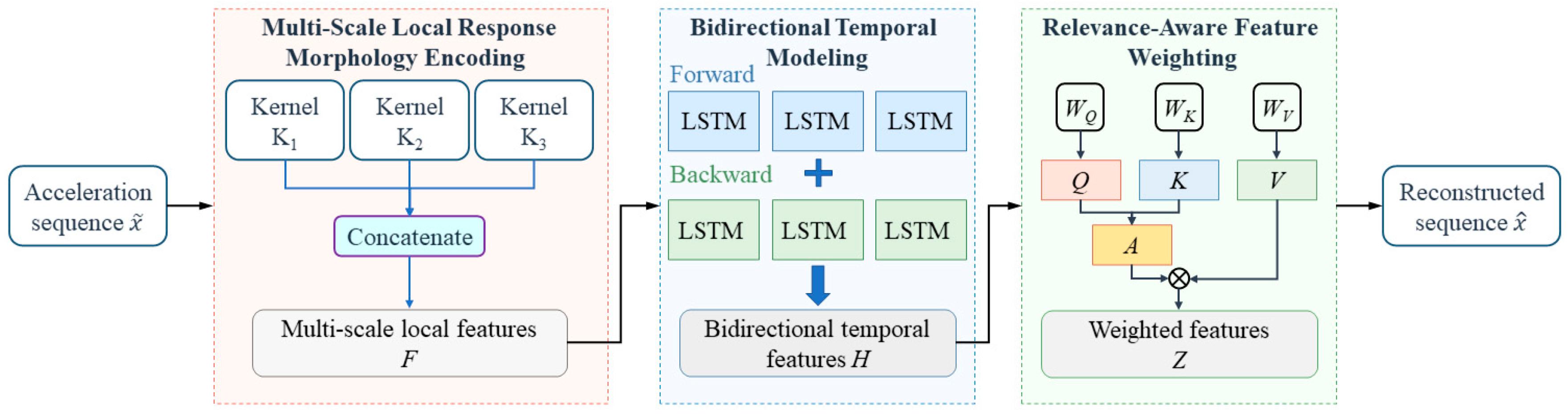
Figure 2.
Finite element model and monitoring-point layout of the offshore platform: (a) Front view; (b) Side view; (c) Top view; (d) Monitoring-point layout on the decks.
Figure 2.
Finite element model and monitoring-point layout of the offshore platform: (a) Front view; (b) Side view; (c) Top view; (d) Monitoring-point layout on the decks.
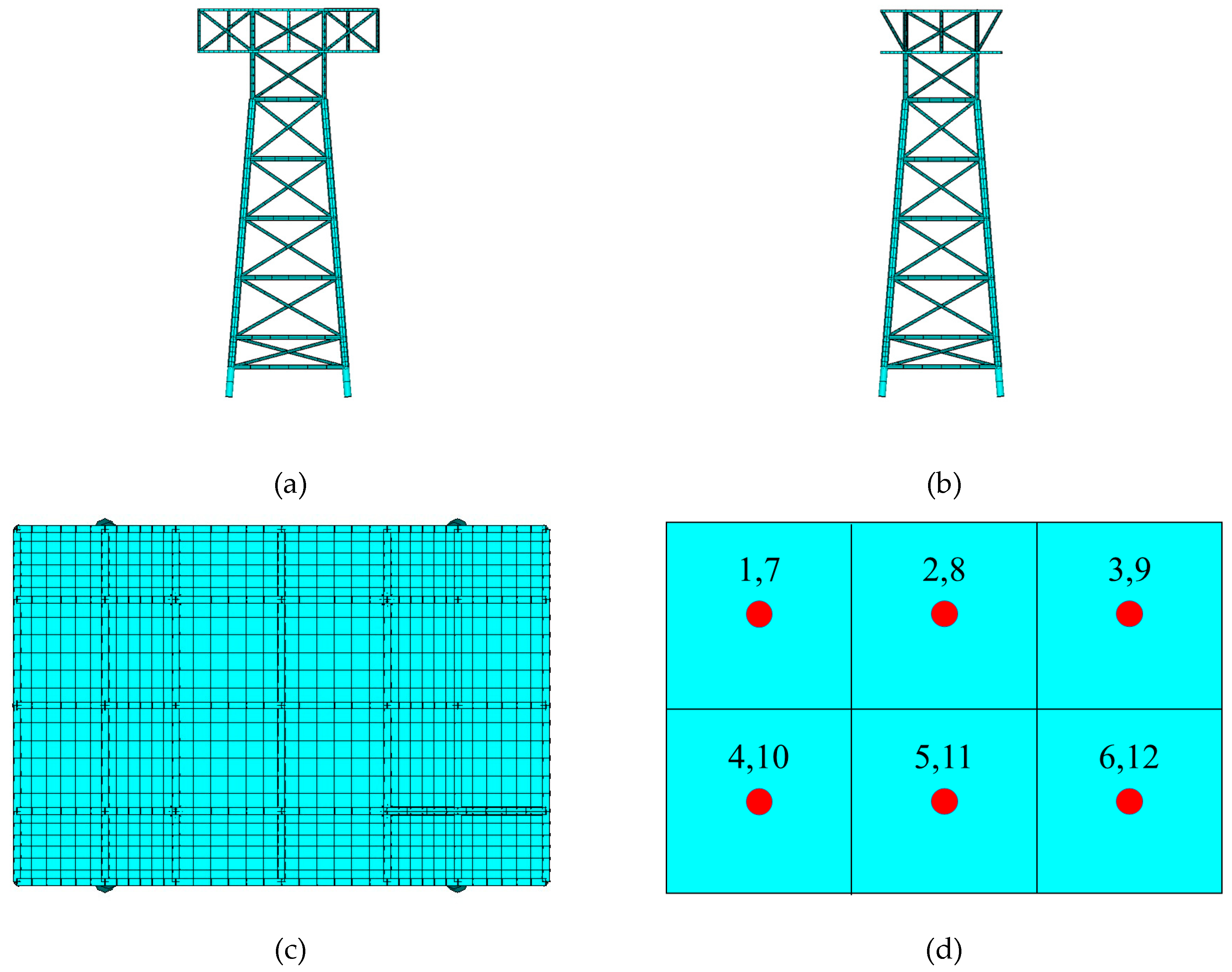
Figure 3.
Training and validation loss curves of the three models: (a) Training loss; (b) Validation loss.
Figure 3.
Training and validation loss curves of the three models: (a) Training loss; (b) Validation loss.
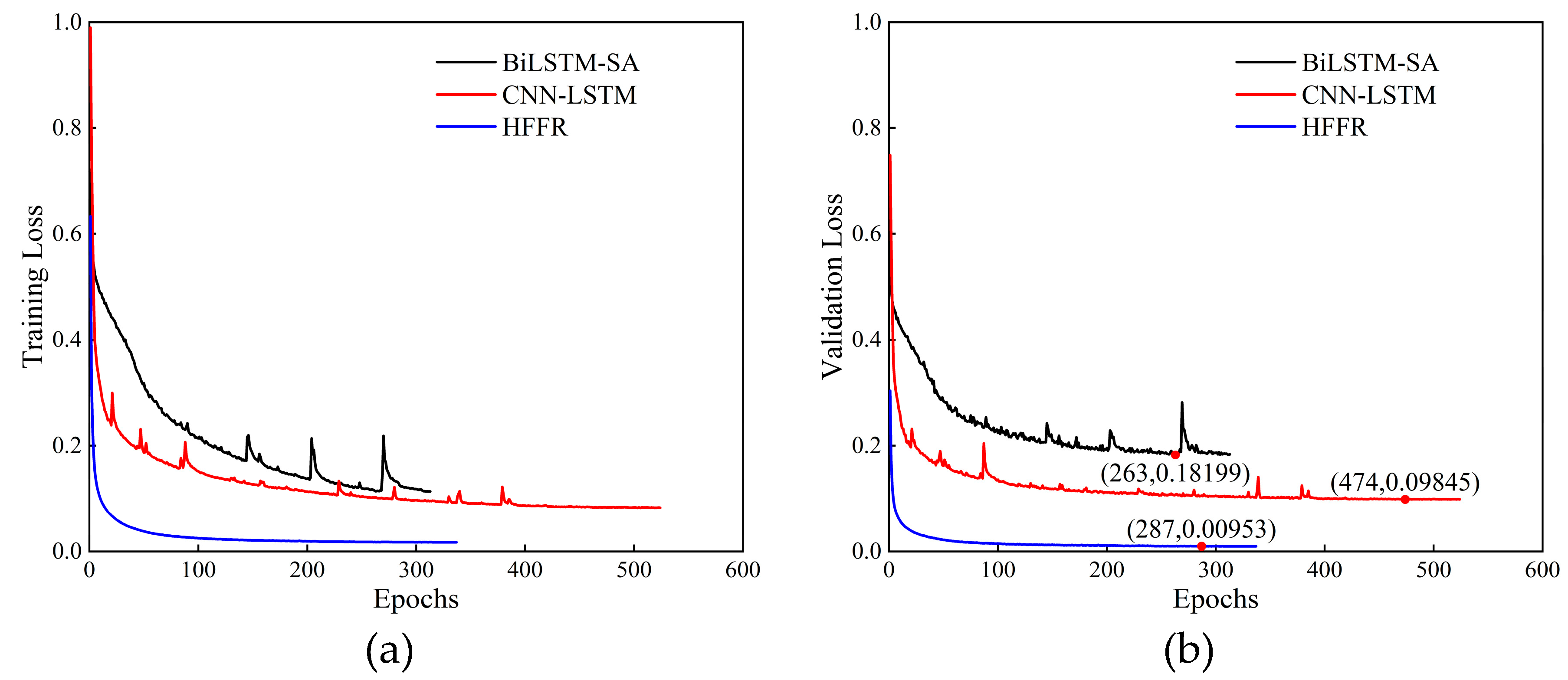
Figure 4.
Comparison between the target and HFFR-reconstructed acceleration responses under different wave–current conditions: (a) Condition 1; (b) Condition 2; (c) Condition 3; (d) Condition 4; (e) Condition 5.
Figure 4.
Comparison between the target and HFFR-reconstructed acceleration responses under different wave–current conditions: (a) Condition 1; (b) Condition 2; (c) Condition 3; (d) Condition 4; (e) Condition 5.
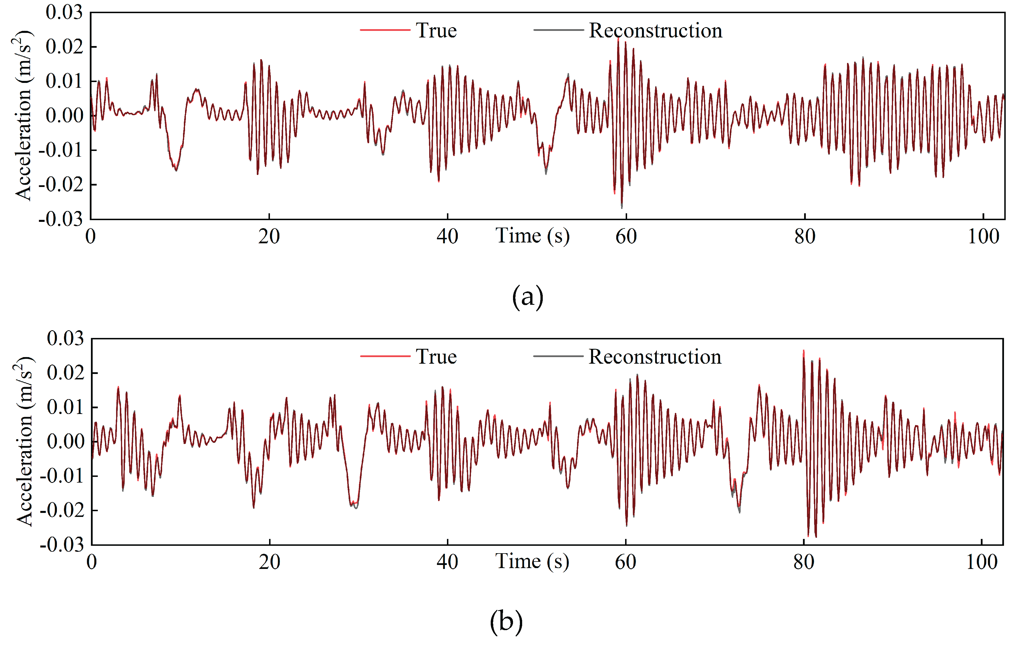
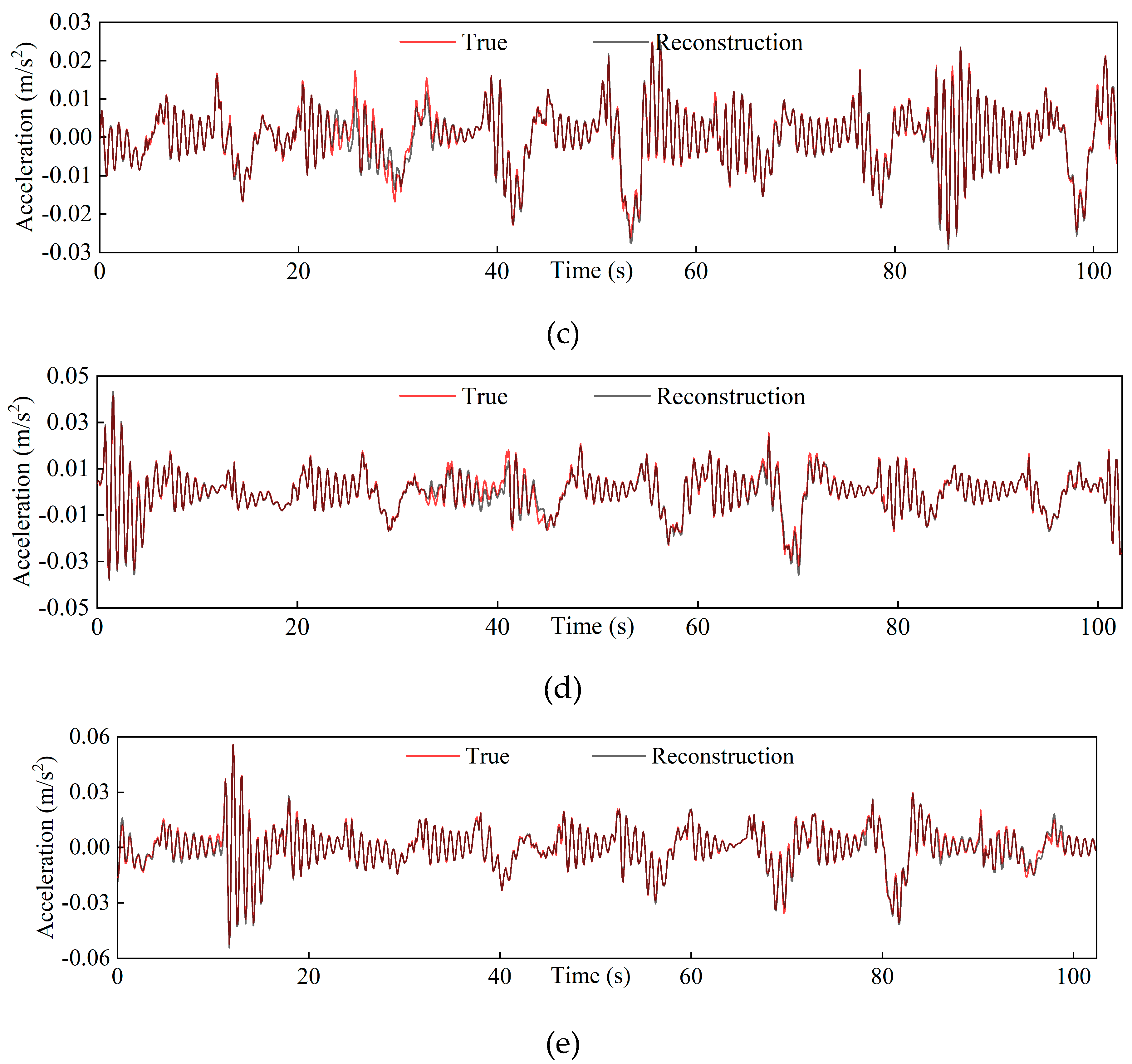
Figure 5.
Comparison of reconstructed acceleration responses in the frequency domain under different wave–current conditions: (a) Condition 1; (b) Condition 2; (c) Condition 3; (d) Condition 4; (e) Condition 5.
Figure 5.
Comparison of reconstructed acceleration responses in the frequency domain under different wave–current conditions: (a) Condition 1; (b) Condition 2; (c) Condition 3; (d) Condition 4; (e) Condition 5.
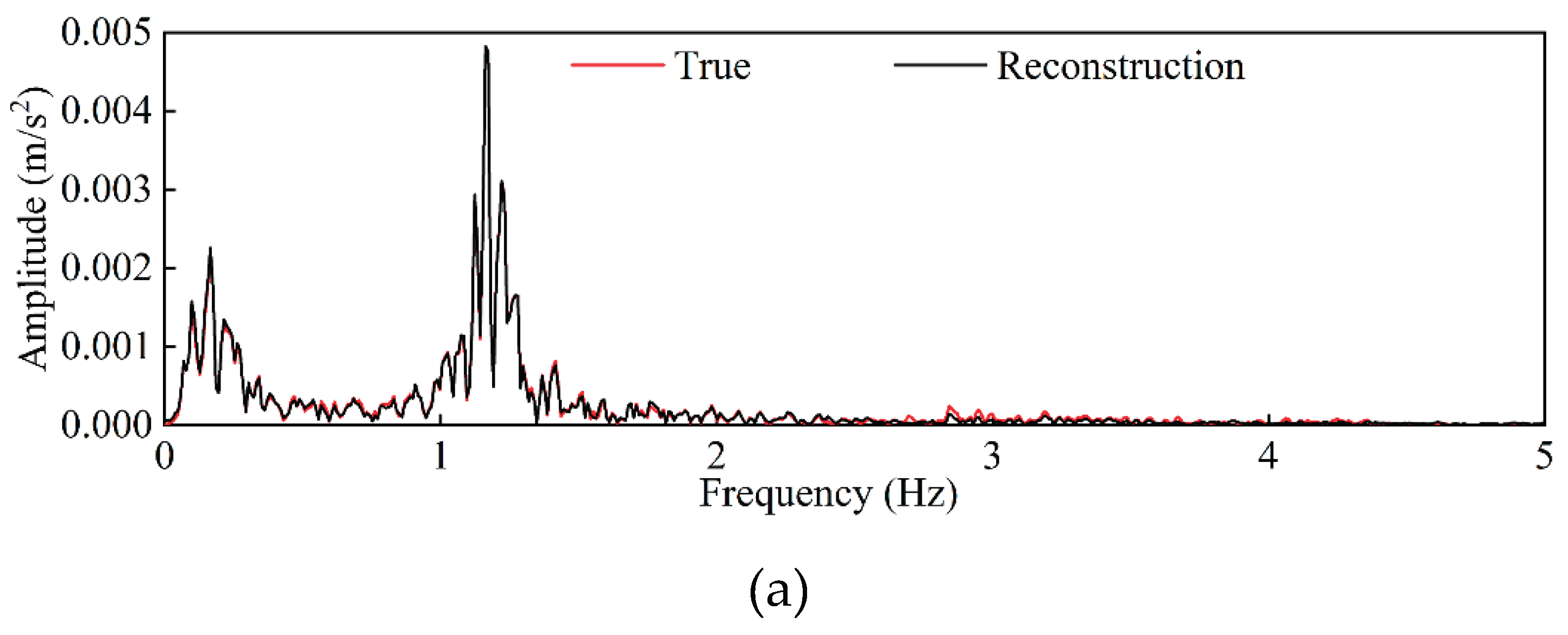
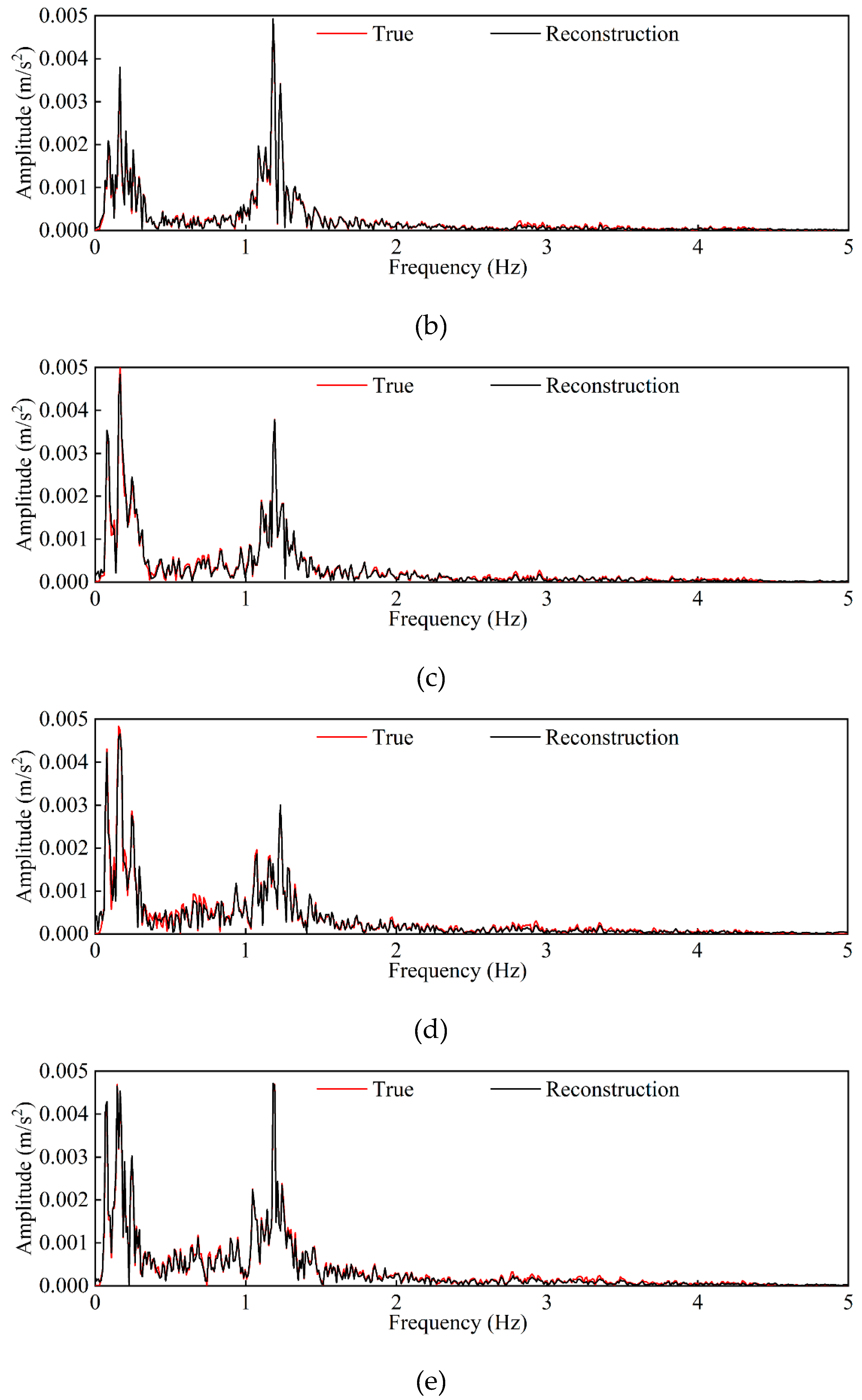
Figure 6.
Scatter plots of target and reconstructed acceleration responses for different models: (a) HFFR; (b) CNN-LSTM; (c) BiLSTM-SA.
Figure 6.
Scatter plots of target and reconstructed acceleration responses for different models: (a) HFFR; (b) CNN-LSTM; (c) BiLSTM-SA.
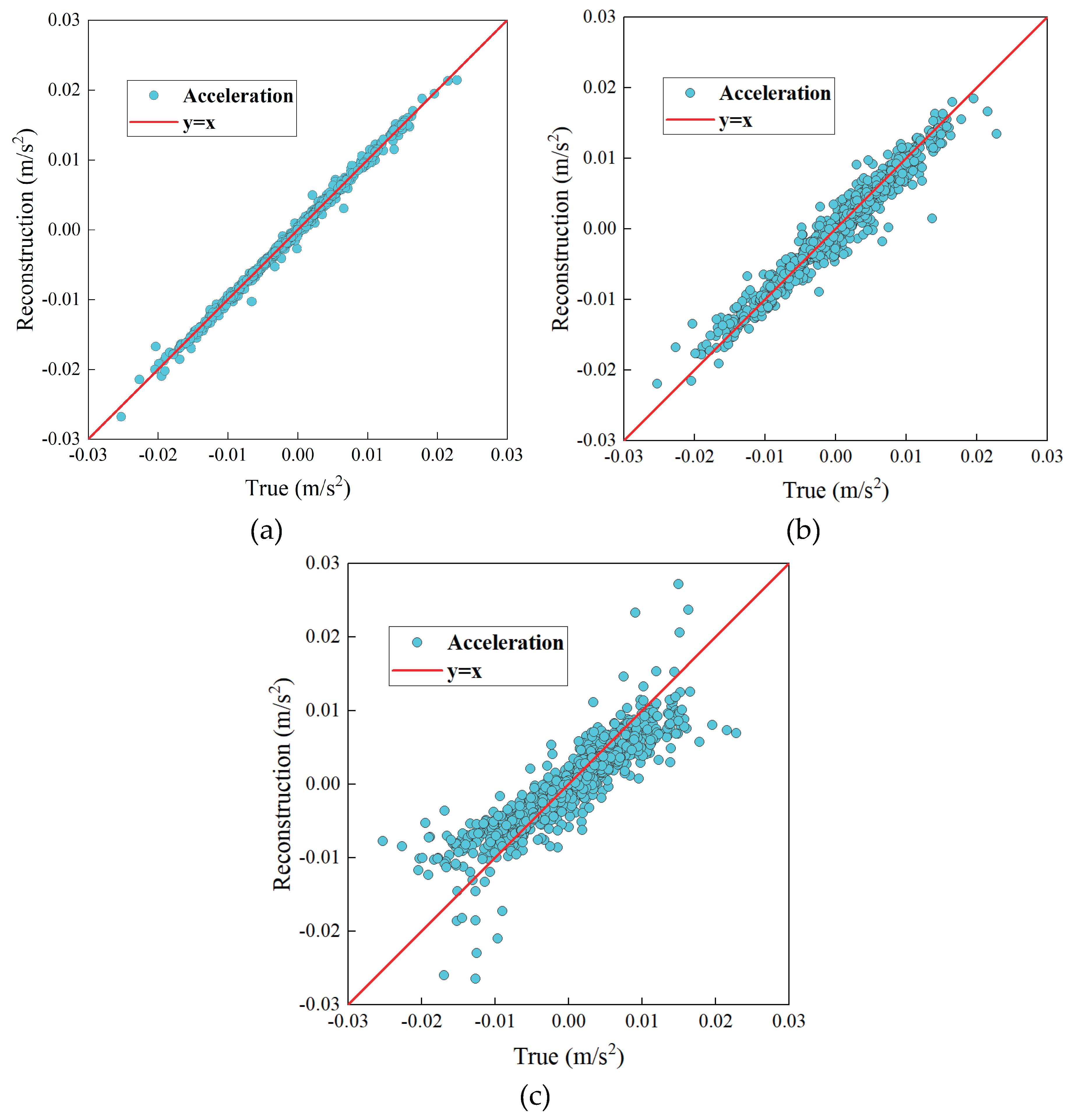

Table 1.
Wave–current condition parameters.
| Condition | Hs [m] | Tp [s] | V [m/s] |
|---|---|---|---|
| 1 | 4.4 | 8.9 | 1.63 |
| 2 | 5.1 | 9.6 | 1.68 |
| 3 | 5.9 | 10.4 | 1.75 |
| 4 | 6.5 | 11.0 | 1.80 |
| 5 | 7.1 | 11.5 | 1.85 |
Table 2.
Ablation configurations and reconstruction performance of HFFR.
| Configuration | BTM | MLME | AFW | RMSE | R2 |
|---|---|---|---|---|---|
| Variant 1 | √ | 0.5036 | 0.7581 | ||
| Variant 2 | √ | √ | 0.2300 | 0.9495 | |
| HFFR | √ | √ | √ | 0.1109 | 0.9883 |
Table 3.
Reconstruction performance of different models.
| Model | RMSE | R2 |
|---|---|---|
| HFFR | 0.1109 | 0.9883 |
| CNN-LSTM | 0.2856 | 0.9222 |
| BiLSTM-SA | 0.5026 | 0.7591 |
Disclaimer/Publisher’s Note: The statements, opinions and data contained in all publications are solely those of the individual author(s) and contributor(s) and not of MDPI and/or the editor(s). MDPI and/or the editor(s) disclaim responsibility for any injury to people or property resulting from any ideas, methods, instructions or products referred to in the content. |
© 2026 by the authors. Licensee MDPI, Basel, Switzerland. This article is an open access article distributed under the terms and conditions of the Creative Commons Attribution (CC BY) license (http://creativecommons.org/licenses/by/4.0/).
Copyright: This open access article is published under a Creative Commons CC BY 4.0 license, which permit the free download, distribution, and reuse, provided that the author and preprint are cited in any reuse.