PySkyLumos: A Python-Based Polarized Skylight Simulator

1. Introduction

Light is electromagnetic radiation that propagates as a transverse wave of mutually perpendicular electric and magnetic fields; the electric field’s oscillation defines the polarization state [1,2,3]. Sunlight is unpolarized before entering the atmosphere, but scattering by air molecules and aerosols generates characteristic polarized sky patterns [4,5,6,7]. As with many other early discoveries it is hard to point exactly when and by whom polarized light was observed or used first. Although systematic optical studies began being documented with Bartholin’s work on Icelandic spar in 1669 [1,2], historical evidence suggests earlier use of polarization cues, such as Viking navigation with “sunstones” [2,3]. Polarization sensitivity is also widespread in the animal kingdom, enabling navigation, scene recognition, and communication [3,8,9,10,11,12]. Inspired by these natural strategies, modern measurement science has increasingly employed polarized light across domains such as remote sensing [13,14], cloud reconstruction [15], navigation [16], material analysis and characterization [17], and even consumer products [18].

Due to its broad applicability, polarized light has become an important research focus. With the rapid growth of artificial intelligence, studies have attempted to combine polarization imaging with machine learning and deep learning methods [13,14,19]. Since humans cannot directly perceive the polarization state of light, dedicated sensors are required [20,21,22]. However, such sensors are often costly, and collecting sufficient measurements for algorithm training is time-consuming. To mitigate these challenges, several polarization image datasets [23,24] and simulators [24,25,26] have been released. Yet, existing datasets typically lack polarization-specific metadata, such as the astronomical positions of singularity points, and current simulators do not provide functionality for generating datasets enriched with this information. Consequently, researchers must invest significant effort into dataset construction and into learning complex astronomical computations (e.g., frame transformations, sun-position algorithms) before they can focus on advancing new studies. Furthermore, none of the available datasets or simulators incorporate the latest skylight polarization model, namely the Pan model [7].

To address this gap, we have developed PySkyLumos [27,28]. It is a self-contained Python toolkit for fast, physically consistent skylight-polarization simulation and sensor emulation. Unlike previously reported tools, it implements the state-of-the-art Pan model [7]. It runs faster than prior Python simulators using modern software methods, and outputs rich metadata, including astronomical locations of polarization singularities to support instrumentation and bio-inspired perception.

The rest of the paper is organized as follows: Section 1.1 reviews related work; Section 2 introduces the Rayleigh, Berry, and Pan models and details the PySkyLumos methodology and implementation; Section 3 reports benchmarks, comparisons to OpenSky, and validation against field measurements; Section 4 discusses their implications; and Section 5 concludes with future directions.

1.1. Related Work

Existing simulators have primarily focus on the Rayleigh and Berry models, and have not included the recently developed Pan model [7]. The Rayleigh model [4], while analytically simple, provides only a coarse approximation of the sky polarization pattern, whereas the Berry model [5,6] offers improved accuracy at the cost of greater complexity. The Pan model can be viewed as an extension to the Berry model, with elevation dependent singularity points positioning.We first summarize recent developments in this area and then outline the key improvements introduced by the present work.

1.1.1. Polarized Skylight Navigation Simulation Dataset (PSNS)

In [24], the authors constructed a polarized-skylight navigation dataset based on the Berry model [5,6] combined with the Hosek luminance model [29,30]. The dataset contains approximately 138,000 images recorded at analyzer orientations of 0, 45, 90, and 135, including both noise-free and noisy variants. It was generated using the hypothetical polarization camera described by prior work [25], together with an external Sun-position model. A Lucid Vision Labs polarization camera [31] incorporating a Sony micropolarizer array [32] was used to inform the sensor model. While several sensor parameters are included, noise characteristics and lens conjugation are not explicitly modeled. Moreover, the dataset does not provide polarization-specific metadata, such as the anti-sun position or the astronomical locations of singularity points and neither does their simulator. The associated C++ software has been made publicly available on GitHub [33,34], although only the Rayleigh sky model is implemented in that release.

1.1.2. OpenSky

OpenSky is the current state-of-the-art Python-based skylight polarization simulator [26], with a parallel MATLAB implementation. It supports both the Rayleigh and Berry models, together with a photometric relative-radiance formulation, namely the CIE model [29,35,36,37,38]. OpenSky’s modular design allows users to choose between purely theoretical physical-model outputs and simulated sensor outputs based on a micro-polarizer imaging sensor, specifically the Sony IMX250MZR [32]. Compared with work described in [24,25], it additionally includes five optical models for the objective lens, as described in [39]. However, as with other work, it does not provide polarization-specific metadata. The simulator was validated experimentally by recording real-world recordings from the Sony sensor in conjunction with standard cameras and comparing them with simulated results.

OpenSky has been released on GitHub [40] for both Python and Matlab, together with a sample Jupyter Notebook illustrating its use. In the example script, the solar vector is fixed at 0 altitude and 84 azimuth, which enforces sky symmetry and yields consistent agreement between theoretical and sensor-modeled outputs. When the solar vector is shifted to asymmetric positions, however, we have found that simulated sensor results deviate from theoretical predictions, highlighting potential limitations in the current implementation for more general scenarios.

1.1.3. Motivation for current work

Building on our analysis of existing simulators, PySkyLumos was designed to address several limitations found in the existing tools, thereby extending the applicability of skylight-polarization simulation. In particular, integrating a solar-ephemeris routine and automated reference-frame calculation eliminates the substantial pre-processing required in both PSNS [24,25] and OpenSky [26]. The PSNS framework [24,25,33,34], although centered on theoretical rendering, could be strengthened by extending its public code base beyond the Rayleigh implementation to include the Berry formulation, consistent with its dataset release. OpenSky [26], by contrast, would benefit from a mosaic-agnostic sensor layer, adoption of the Pan model [7], and fuller use of Python’s vectorized numerical libraries to improve throughput. Both platforms would also gain from incorporating polarization-specific metadata, such as singularity-point positions, as it enables more precise downstream analysis. Together, these enhancements would broaden the scientific utility of such tools while reducing barriers to their effective use.

2. Materials and Methods

2.1. Skylight Polarization Models

This section introduces the principal analytical models [4,5,6,7] of the skylight polarization distribution. The distribution of skylight polarization is determined primarily by the solar position [2,7,9,22,24,26]. Our study focuses on analytical rather than numerical formulations, as they offer greater computational efficiency and this allow direct access to polarization-specific metadata. Although the Wilkie model [35] has seen wide use in computer graphics, it is excluded here because it cannot represent key physical features of skylight polarization, such as the neutral points, as noted by its authors [35]. The skylight polarization distribution is characterized by 2 parameters, the degree of polarization (DOP) and the angle of polarization (AOP). The DOP quantifies the fraction of light that is polarized, while the AOP specifies the orientation of the electric field’s vibration direction [1,2,3,4,5,6,7].

2.1.1. Rayleigh

The Rayleigh model [4] provides the simplest analytical description of skylight polarization and is historically the earliest framework used. It characterizes scattering by atmospheric particles much smaller than the wavelength of light, which results in stronger scattering at shorter wavelengths [22,24,26]. This wavelength dependence explains the blue appearance of the daytime sky and the red hues observed at sunrise and sunset [4]. The model assumes that sunlight undergoes single elastic scattering by isotropic, homogeneous spherical molecules, thereby neglecting multiple scattering and atmospheric inhomogeneities. While useful for its simplicity, the Rayleigh model predicts only two neutral points (locations where the degree of linear polarization vanishes), situated in the solar and anti-solar directions [22,24,26].

2.1.2. Berry

The Berry sky model extends the Rayleigh formulation by incorporating multiple scattering and atmospheric turbidity through the framework of singularity theory [5,6]. This leads to the appearance of four neutral points, named after their discoverers: Brewster (below the Sun), Babinet (above the Sun), Arago (above the anti-Sun), and the Horváth or “Fourth” point (below the anti-Sun) [3]. These neutral points are located approximately 15° above and below the solar and anti-solar directions, yielding a closer match to observed polarization distributions. In addition, the Berry model captures the displacement and asymmetry of neutral points under varying atmospheric conditions, such as partial cloud cover, thereby offering a more realistic description of skylight polarization patterns [5,6,24,26].

2.1.3. Pan

The Pan model can be seen as an extension of the Berry model. Towards the horizon, the increased atmospheric thickness leads to stronger scattering effects [7,26]. In Berry’s model, the Sun and anti-Sun are positioned midway between their corresponding neutral points, which are assumed to remain at a fixed angular distance [5,6,7]. In reality, this angular separation varies with solar elevation due to the influence of atmospheric thickness [7,26]. The Pan model explicitly incorporates this variability, extending the Berry formulation to account for the shifting positions of neutral points and thereby providing a more accurate representation of observed skylight polarization patterns [7].

2.2. Methodology

This section describes the software structure and methodology, with emphasis on four major improvements: integration of solar-ephemeris modeling, generation of polarization-specific image metadata, enhancement of computational efficiency, and implementation of the skylight polarization models. We begin by detailing the use of vectorization and broadcasting techniques to accelerate processing. We then describe the incorporation of Sun trajectory calculations to automate ephemeris handling and the generation of polarization-specific metadata, including parameters such as singularity-point positions. Finally, we present the implementation of the skylight polarization models, including the latest model, extending the simulator’s physical fidelity.

OpenAI Codex and ChatGPT, using GPT-4o, were used for code review and documentation generation during the preparation of PySkyLumos and its documentation.

2.2.1. Computational Efficiency Enhancement

PySkyLumos achieves near C-level performance by leveraging NumPy’s vectorized operations and broadcasting, built on high-performance back-ends. NumPy enables efficient vectorized computation by combining broadcasting—automatic alignment of array shapes without redundant copies—with SIMD (single instruction multiple data) based operations that apply a single instruction to multiple data elements simultaneously [41,42].

PySkyLumos introduces the SlicingPattern class, a data class [43] that encodes the start row, start column, and step of each analyzer type in the micro-polarizer array. Serving as the core of the StokesCalculator. It enables vectorized operations, efficient polarization-parameter extraction, and flexible support for arbitrary sensor mosaics. This contrasts with OpenSky [26], which relies on nested loops and hard-coded sensor layouts. However, the sensor, micro-polarizer array, and lens models in [26,39] follow well-established textbook formulations and were therefore adopted directly in our implementation.

2.2.2. Sun Trajectory and Polarization Metadata

PySkyLumos uses Astropy [44] to compute Sun motion and perform WGS84 frame transformations [45], where WGS84 is the standard Earth reference ellipsoid for geodetic positioning. By default, it applies the VSOP2000 analytical ephemeris [46], accurate to about 4 km over 1900–2100 C.E., with optional JPL ephemerides [47] for higher precision at greater cost. Both yield a SkyCoord object in the GCRS frame, representing geocentric celestial coordinates, which is then converted to the local altitude–azimuth frame. PySkyLumos simplifies this process by exposing only the ephemeris selection to the user.

Through its integration with Astropy, PySkyLumos provides a methodological capability absent from comparable tools. Each simulated image is enriched with model-specific polarization metadata, including the scattering angle, Sun and anti-Sun positions, and singularity point coordinates defined by the selected sky model, according to their placement on the great circle connecting the observer and the Sun [48,49].

2.2.3. Skylight Polarization Models

PySkyLumos implements the standard Rayleigh and Berry skylight polarization models [4,5,6]. For the Rayleigh model, the AOP and DOP are computed as:

$$\begin{array}{cc}\hfill N& =\sin {\theta }_p\sin {\theta }_s\cos ({\alpha }_p-{\alpha }_s)-\cos {\theta }_p\sin {\theta }_s,\hfill \\ \hfill D& =\cos {\theta }_s\sin ({\alpha }_p-{\alpha }_s),\hfill \\ \hfill AOP& ={\tan }^{-1}\left[\tan \left({\tan }^{-1}{\displaystyle \frac{N}{D}}+{\alpha }_p\right)\right],\hfill \\ \hfill DOP& ={\displaystyle \frac{{\sin }^2\gamma }{1+{\cos }^2\gamma }}DO{P}_{max}.\hfill \end{array}$$

(1)

here ${\theta }_p$ and ${\alpha }_p$ are the altitude and azimuth of the observation point, ${\theta }_s$ and ${\alpha }_s$ are the Sun altitude and azimuth, and $\gamma$ is the scattering angle.

The Berry model is more complex. Using the observer’s zenith angle ${\phi }_p$, the Sun’s zenith angle ${\phi }_s$, and the angular distance between singularities $\delta$, which we have set as 30 as it is the middle value of the ranges provided by previous research [5,6,48,49], the complex projections are:

$$\begin{array}{cc}\hfill \xi & =\tan {\displaystyle \frac{{\phi }_p}{2}}{e}^{i{\alpha }_p},\hfill \\ \hfill {\xi }_{+}& =e^{i{\alpha }_s}{\displaystyle \frac{\tan \frac{{\phi }_s}{2}+\tan \frac{\delta }{4}}{1-\tan \frac{{\phi }_s}{2}\tan \frac{\delta }{4}}},\hfill \\ \hfill {\xi }_{-}& =e^{i{\alpha }_s}{\displaystyle \frac{\tan \frac{{\phi }_s}{2}-\tan \frac{\delta }{4}}{1+\tan \frac{{\phi }_s}{2}\tan \frac{\delta }{4}}}.\hfill \end{array}$$

(2)

the transformation $\xi \mapsto \omega \left(\xi \right)$ is:

$$\omega \left(\xi \right)={\displaystyle \frac{4(\xi -{\xi }_{+})(\xi -{\xi }_{-})(\xi +{\xi }_{+}^{*})(\xi +{\xi }_{-}^{*})}{{(1+|\xi |}^2{)}^2|{\xi }_{+}+1/{\xi }_{+}^{*}\left|\right|{\xi }_{-}+1/{\xi }_{-}^{*}|}}.$$

(3)

finally, the angle and degree of polarization are:

$$\begin{array}{cc}\hfill AOP& =\frac{1}{2}\arg \left[\omega \left(\xi \right)e^{-2i{\alpha }_s}\right],\hfill \\ \hfill DOP& ={\displaystyle \frac{\left|\omega \right(\xi \left)\right|}{2-\left|\omega \right(\xi \left)\right|}}DO{P}_{max}.\hfill \end{array}$$

(4)

The Pan model [7] extends the Berry model [5,6] by allowing the angular separation of the singularity points to vary with the Sun’s altitude. Accordingly, PySkyLumos implements the Pan model by replacing the Berry parameter ${\displaystyle \frac{\delta }{4}}$ with elevation-dependent terms that differ for the Brewster and Babinet projections. The angular distances between the Sun and the Brewster and Babinet points as functions of solar altitude are given by:

$$\begin{array}{cc}\hfill {\delta }_{\mathrm{Babinet}}\left({\theta }_s\right)& =42.53-0.56·{\theta }_s\hfill \\ \hfill {\delta }_{\mathrm{Brewster}}\left({\theta }_s\right)& =\left\{\begin{array}{cc}56.84-0.25·{\theta }_s,\hfill & {\theta }_s\ge {27}^{\circ }\hfill \\ 37.34+0.49·{\theta }_s,\hfill & {\theta }_s\le {27}^{\circ }\hfill \end{array}\right.\hfill \end{array}$$

(5)

where ${\delta }_{Brewster}$ and ${\delta }_{Babinet}$ denote the angular distances between the Sun and the Brewster and Babinet points, respectively. Using these elevation dependent distances in place of Berry’s constant parameter yields the following expression:

$$\begin{array}{cc}\hfill & {\xi }_{+}=e^{i{\alpha }_s}{\displaystyle \frac{\tan \left(\frac{{\phi }_s}{2}\right)+\tan \left(\frac{{\delta }_{Brewster}}{2}\right)}{1-\tan \left(\frac{{\phi }_s}{2}\right)·\tan \left(\frac{{\delta }_{Brewster}}{2}\right)}}\hfill \\ \hfill & {\xi }_{-}=e^{i{\alpha }_s}{\displaystyle \frac{\tan \left(\frac{{\phi }_s}{2}\right)-\tan \left(\frac{{\delta }_{Babinet}}{2}\right)}{1+\tan \left(\frac{{\phi }_s}{2}\right)·\tan \left(\frac{{\delta }_{Babinet}}{2}\right)}}\hfill \end{array}$$

(6)

where the halving follows from the stereographic projection, which maps a true sky angle $\delta$ on the sphere to the complex plane radius as $\tan \left({\displaystyle \frac{\delta }{2}}\right)$; unlike Berry’s constant split, where each singularity is offset by half the pairwise separation, giving ${\displaystyle \frac{\delta }{4}}$, Pan directly uses the individual Sun–singularity distances, requiring only the division by 2.

3. Results

This section presents the results obtained with the PySkyLumos software and comparisons against OpenSky [26]. It first reports processing-speed benchmarks on Apple-silicon and Intel-based systems, followed by a performance comparison with OpenSky using the same evaluation procedure. Finally, the Pan model implementation is validated against real-world recordings from a commercial polarization camera.

3.1. Computational Efficiency Enhancement

Each simulation was run ten times with identical parameters, and average, minimum, and maximum times were recorded. OpenSky’s meridian-frame AOP step was omitted for fairness. Benchmarks were conducted on a 2024 MacBook Pro (M4 Pro, 14 cores, 24 GB RAM) and an HP EliteBook 850 G8 (i5-1135G7, 4 cores/8 threads, 16 GB RAM). Results are shown in the tables below.

Table 1 and Table 2 show that PySkyLumos achieves substantially higher computational efficiency than OpenSky while providing additional frame calculations, polarization specific metadata, and Sun-motion modeling. On both test platforms, the overall simulation time is reduced by roughly a factor of five on average. The largest gain occurs in the Stokes-parameter image formation, where PySkyLumos executes on average approximately 100 times faster than OpenSky on the MacBook and 124 on the Windows PC.

Table 1. Overall software simulation runtime on a Windows PC (s).

	PySkyLumos			OpenSky
	Rayleigh	Berry	Pan	Rayleigh	Berry
MIN	2.86	3.03	3.08	13.69	13.87
AVG	3.06	3.24	3.29	15.47	15.65
MAX	3.36	3.45	3.57	22.90	24.76

Table 1. Overall software simulation runtime on a Windows PC (s).

	PySkyLumos			OpenSky
	Rayleigh	Berry	Pan	Rayleigh	Berry
MIN	2.86	3.03	3.08	13.69	13.87
AVG	3.06	3.24	3.29	15.47	15.65
MAX	3.36	3.45	3.57	22.90	24.76

Table 2. Overall software simulation runtime on an Apple M4 Pro (s).

	PySkyLumos			OpenSky
	Rayleigh	Berry	Pan	Rayleigh	Berry
MIN	0.66	0.67	0.66	3.41	3.42
AVG	0.67	0.68	0.67	3.45	3.49
MAX	0.69	0.68	0.69	3.53	3.55

Table 2. Overall software simulation runtime on an Apple M4 Pro (s).

	PySkyLumos			OpenSky
	Rayleigh	Berry	Pan	Rayleigh	Berry
MIN	0.66	0.67	0.66	3.41	3.42
AVG	0.67	0.68	0.67	3.45	3.49
MAX	0.69	0.68	0.69	3.53	3.55

Table 3. Stokes-parameter image formation runtime on a Windows PC (s).

	PySkyLumos			OpenSky
	Rayleigh	Berry	Pan	Rayleigh	Berry
MIN	0.054	0.055	0.056	10.59	10.68
AVG	0.057	0.058	0.059	10.74	10.87
MAX	0.06	0.06	0.06	10.98	11.5

Table 3. Stokes-parameter image formation runtime on a Windows PC (s).

	PySkyLumos			OpenSky
	Rayleigh	Berry	Pan	Rayleigh	Berry
MIN	0.054	0.055	0.056	10.59	10.68
AVG	0.057	0.058	0.059	10.74	10.87
MAX	0.06	0.06	0.06	10.98	11.5

Table 4. Stokes-parameter image formation runtime on an Apple M4 Pro (s).

	PySkyLumos			OpenSky
	Rayleigh	Berry	Pan	Rayleigh	Berry
MIN	0.017	0.017	0.017	2.62	2.71
AVG	0.018	0.018	0.018	2.65	2.72
MAX	0.019	0.021	0.022	2.69	2.74

Table 4. Stokes-parameter image formation runtime on an Apple M4 Pro (s).

	PySkyLumos			OpenSky
	Rayleigh	Berry	Pan	Rayleigh	Berry
MIN	0.017	0.017	0.017	2.62	2.71
AVG	0.018	0.018	0.018	2.65	2.72
MAX	0.019	0.021	0.022	2.69	2.74

3.2. Skylight Polarization Models Extension

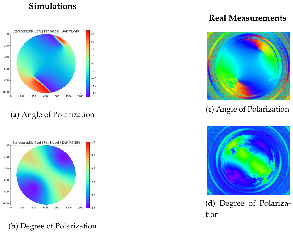
To validate the simulator, measurements were taken at two sites: University of Liverpool, UK (53.4052, $-2.9650$) on 11 Nov 2024 at 12:52 and Iancului–Pantelimon, Bucharest, Romania (44.4427, 26.1491) on 11 Jan 2025 at 15:47. A Thorlabs 5 MP Kiralux polarization-sensitive CMOS camera with a polarizer array and a Fujinon FE185C057HA-1 [50] 1.8 mm f/1.4 fisheye lens (185 field of view) was used. Recordings are shown below in the order Liverpool-Bucharest.

Figure 1. Comparison between PySkyLumos images and measurements from Liverpool. Top of each image points East.

Figure 1. Comparison between PySkyLumos images and measurements from Liverpool. Top of each image points East.

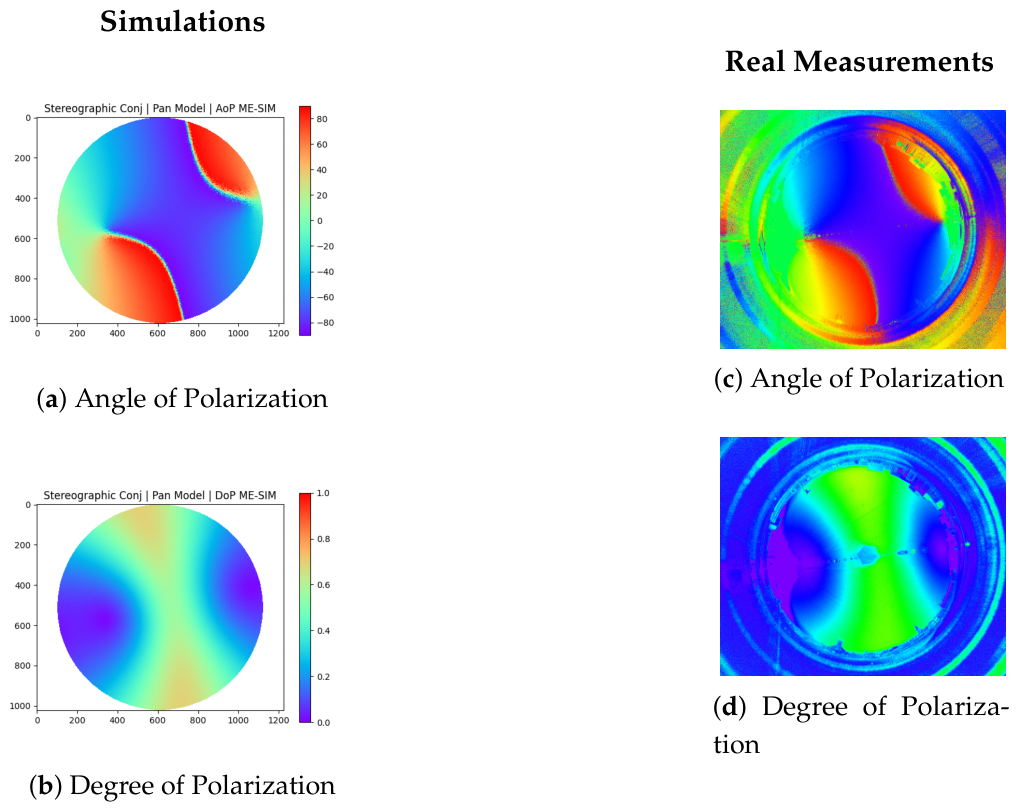
Figure 2. Comparison between PySkyLumos images and measurements from Bucharest. Top of each image points East.

Figure 2. Comparison between PySkyLumos images and measurements from Bucharest. Top of each image points East.

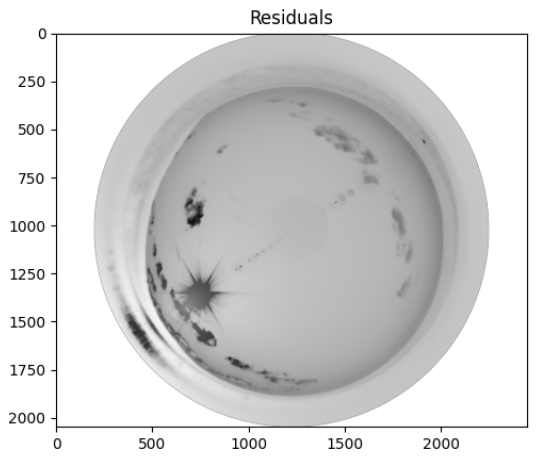
For a quantitative analysis, additional data were collected in Belmont, UK (lat 53.6358, lon -2.5222) on 22^nd of September 2025 at 15:05 UTC to extract the angle and degree of polarization from the raw bits images. The Belmont simulation used seed of 9, a 15 azimuthal rotation, the Pan sky model, a CIE value of 8, a 1 altitude clipping, and the parameters of the sensor built mentioned above. The visual results can be observed below along with the simulation residuals where the darker areas indicate mismatches:

Figure 3. Comparison between PySkyLumos raw bits image and measurements from Belmont. Top of each image points East.

Figure 3. Comparison between PySkyLumos raw bits image and measurements from Belmont. Top of each image points East.

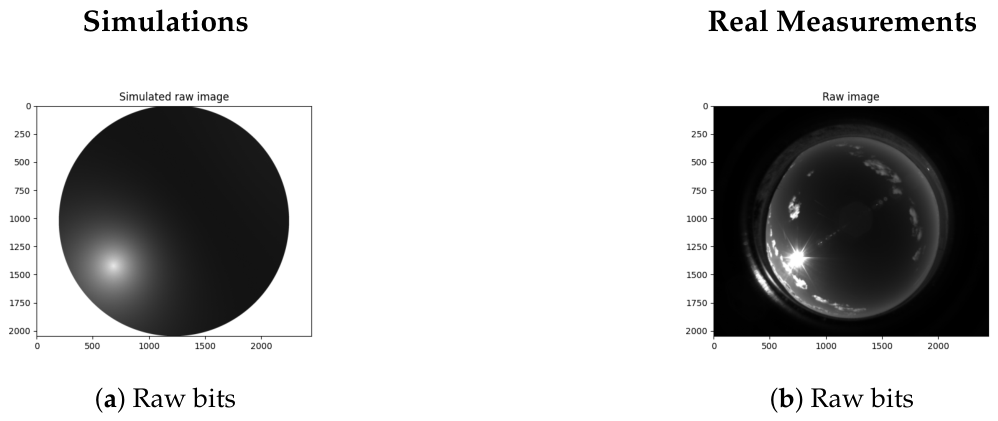
Both mean absolute error (MAE) and root mean square error (RMSE) were computed to capture average deviations and outlier effects, with normalized values reported for the angle of polarization. The raw image simulation produced an MAE of 351 and an RMSE of 503.7; the degree of polarization yielded an MAE of 0.14 and an RMSE of 0.16; and the angle of polarization showed an MAE of 2.69 (normalized 0.0075) and an RMSE of 14.95 (normalized 0.041). The errors were normalized by the maximum possible angular difference, allowing for scale-independent comparison.

4. Discussion

This level of acceleration enables the generation of large-scale synthetic datasets and real-time testing scenarios that were previously impractical. For example, producing millions of sky-polarization frames for deep-learning model training can now be completed in hours instead of days, and real-time sensor simulation becomes feasible.

Figure 4 shows that the largest errors arise from clouds, Sun glare, and overlapping Sun rays, which are outside the scope of the current study but important for future updates.

5. Conclusions

This work has introduced PySkyLumos, an open-source Python framework for generating physically accurate skylight-polarization data with associated astronomical metadata. It implements the Rayleigh, Berry, and Pan models to capture both fundamental scattering and elevation-dependent singularity motion. By integrating Astropy’s solar-ephemeris routines and automated frame transformations, PySkyLumos produces polarization maps and singularity locations without the manual pre-processing required by previous tools.

Benchmarking against OpenSky showed that PySkyLumos achieves fivefold faster overall simulation and up to 100× faster Stokes-parameter formation across Apple and Intel platforms. Validation with data from Liverpool, Bucharest, and Belmont confirmed close agreement with real measurements, with errors mainly due to atmospheric effects such as clouds and Sun glare.

Combining high computational efficiency with modern Python design and advanced sky-polarization models, PySkyLumos provides a practical foundation for dataset generation, algorithm development, and instrument testing, with direct relevance to animal vision, bio-inspired computer vision, navigation, robotics, and atmospheric sensing. This makes PySkyLumos a practical tool for rapid prototyping, algorithm benchmarking, and instrument design in polarization-based systems.

References

- Collett, E. Field guide to polarization; SPIE press Bellingham, 2005; Vol. 15. [Google Scholar]
- Goldstein, D.H. Polarized Light, 3rd ed.; CRC Press: Boca Raton, FL, USA, 2017. [Google Scholar] [CrossRef]
- Horváth, G. Polarization Vision and Environmental Polarized Light; Springer Nature, 2024. [Google Scholar] [CrossRef]
- Young, A.T. Rayleigh scattering. Phys. Today 1982, 35, 42–48. [Google Scholar] [CrossRef]
- Berry, M.; Dennis, M.; Lee, R. Polarization singularities in the clear sky. New J. Phys. 2004, 6, 162. [Google Scholar] [CrossRef]
- Berry, M. Nature’s optics and our understanding of light. Contemp. Phys. 2015, 56, 2–16. [Google Scholar] [CrossRef]
- Pan, P.; Wang, X.; Yang, T.; Pu, X.; Wang, W.; Bao, C.; Gao, J. High-similarity analytical model of skylight polarization pattern based on position variations of neutral points. Opt. Express 2023, 31, 15189–15203. [Google Scholar] [CrossRef] [PubMed]
- Waterman, T.H. Polarized light and animal navigation. Sci. Am. 1955, 193, 88–95. [Google Scholar] [CrossRef]
- Waldvogel, J.A. The Bird’s Eye View. Am. Sci. 1990, 78, 342–353. [Google Scholar]
- Wehner, R.d. Polarized-light navigation by insects. Sci. Am. 1976, 235, 106–115. [Google Scholar] [CrossRef] [PubMed]
- van den Berg, C.P.; Troscianko, J.; Endler, J.A.; Marshall, N.J.; Cheney, K.L. Quantitative Colour Pattern Analysis (QCPA): A comprehensive framework for the analysis of colour patterns in nature. Methods Ecol. Evol. 2020, 11, 316–332. [Google Scholar] [CrossRef]
- Cronin, T.W.; Shashar, N.; Caldwell, R.L.; Marshall, J.; Cheroske, A.G.; Chiou, T.H. Polarization Vision and Its Role in Biological Signaling. Integr. Comp. Biol. 2003, 43, 549–558. [Google Scholar] [CrossRef]
- Wang, Y.; Cai, J.; Louie, D.C.; Lui, H.; Lee, T.K.; Jane Wang, Z. Classifying Melanoma and Seborrheic Keratosis Automatically with Polarization Speckle Imaging. In Proceedings of the 2019 IEEE Global Conference on Signal and Information Processing (GlobalSIP), 2019; pp. 1–4. [Google Scholar] [CrossRef]
- Rodríguez-Cortés, O.I.; Martínez-Ponce, G. Towards Skin Lesion Classification Using Machine Learning Algorithms and Stokes Imaging Polarimetry. In Proceedings of the 2024 Conference on Lasers and Electro-Optics Pacific Rim (CLEO-PR), 2024; pp. 1–2. [Google Scholar] [CrossRef]
- Liu, Y.; Long, Y.; Cao, Y.; Liu, W.; Li, W. Three-dimensional model of cloud layers based on all-sky polarization imaging data. In Proceedings of the Ninth Symposium on Novel Photoelectronic Detection Technology and Applications; Chu, J., Liu, W., Xu, H., Eds.; International Society for Optics and Photonics, SPIE, 2023; Vol. 12617, p. 126171K. [Google Scholar] [CrossRef]
- Li, G.; Zhang, Y.; Fan, S.; Yu, F.; Wang, Y. Dynamic-Wave Interference Suppression Based on Angular Increment Assistance for Underwater Imaging Polarization Sensor. IEEE Trans. Instrum. Meas. 2025, 74, 1–13. [Google Scholar] [CrossRef]
- Su, F.; Wu, S.; Zhang, Z. A brief review of the photoelasticity based on a pixelated polarization camera: principle, advantages/disadvantages and typical applications http://arxiv.org/abs/https://academic.oup.com/jom/article-pdf/doi/10.1093/jom/ufae051/61156112/ufae051.pdfhttp://arxiv.org/abs/https://http://arxiv.org/abs/https://academic.oup.com/jom/article-pdf/doi/10.1093/jom/ufae051/61156112/ufae051.pdfhttp://arxiv.org/abs/. J. Mech. 2024, 40, 698–710. Available online: https://academic.oup.com/jom/article-pdf/doi/10.1093/jom/ufae051/61156112/ufae051.pdf][https://academic.oup.com/jom/article-pdf/doi/10.1093/jom/ufae051/61156112/ufae051.pdf. [CrossRef]
- Choi, S.K.; Yang, Y.J.; Kim, K.N.; Choi, J.W.; Choi, Y.J.; Han, S.H. A Study of the Optical Properties of Cosmetics Measured by Polarized Light Goniophotometry. J. Opt. Soc. Korea 2012, 16, 36–41. [Google Scholar] [CrossRef]
- Xu, X.; Wu, J.; Wang, J.; Qu, Q.; Tan, Z.; Luo, M. Materials Identification of Polarized Pulse Laser Detection Based on Sparse Autoencoder and Softmax Classifier Framework. IEEE Trans. Instrum. Meas. 2022, 71, 1–9. [Google Scholar] [CrossRef]
- Karman, S.B.; Diah, S.Z.M.; Gebeshuber, I.C. Bio-inspired polarized skylight-based navigation sensors: A review. Sensors 2012, 12, 14232–14261. [Google Scholar] [CrossRef] [PubMed]
- Li, S.; Kong, F.; Xu, H.; Guo, X.; Li, H.; Ruan, Y.; Cao, S.; Guo, Y. Biomimetic Polarized Light Navigation Sensor: A Review. Sensors 2023, 23, 5848. [Google Scholar] [CrossRef] [PubMed]
- Fang, K.; Yingjing, G.; Zhang, J.; Xiaojing, F.; Xiaohan, G. Review on bio-inspired polarized skylight navigation. Chin. J. Aeronaut. 2023, 36, 14–37. [Google Scholar] [CrossRef]
- Poughon, L.; Aubry, V.; Monnoyer, J.; Viollet, S.; Serres, J.R. An extended database of annotated skylight polarization images covering a period of two months. BMC Res. Notes 2024, 17, 306. [Google Scholar] [CrossRef] [PubMed]
- Liang, H.; Bai, H. Polarized skylight navigation simulation (PSNS) dataset. arXiv 2020, arXiv:2007.13081. [Google Scholar]
- Liang, H.; Bai, H.; Liu, N.; Shen, K. Limitation of Rayleigh sky model for bioinspired polarized skylight navigation in three-dimensional attitude determination. Bioinspiration Biomim. 2020, 15, 046007. [Google Scholar] [CrossRef] [PubMed]
- Moutenet, A.; Poughon, L.; Toulon, B.; Serres, J.R.; Viollet, S. OpenSky: a modular and open-source simulator of sky polarization measurements. IEEE Trans. Instrum. Meas. 2024, 73, 1–16. [Google Scholar] [CrossRef]
- Ciochirca, T.A.; Chadwick, D.J.; Sandall, I.; Ralph, J.F. PySkyLumos (GitHub). 2025. Version as of September 2025.
- Ciochirca, T.A.; Chadwick, D.J.; Sandall, I.; Ralph, J.F. PySkyLumos (Python Package Index). Version. 2025.
- Hosek, L.; Wilkie, A. An analytic model for full spectral sky-dome radiance. ACM Trans. Graph. (TOG) 2012, 31, 1–9. [Google Scholar] [CrossRef]
- Hošek, L.; Wilkie, A. Adding a solar-radiance function to the hošek-wilkie skylight model. IEEE Comput. Graph. Appl. 2013, 33, 44–52. [Google Scholar] [CrossRef] [PubMed]
- LUCID Vision Labs. Phoenix 5.0 MP Polarization Camera (Sony IMX250MZR/MYR). 2024. (accessed on 2024-05-23).
- Sony Semiconductor Solutions Corporation. IMX250/264/253MZR/MYR: Polarization Image Sensor with Four-Directional on-chip Polarizer and global shutter function. Product flyer. Sony Semiconductor Solutions Corporation, 2021. (accessed on 2024-05-23).
- Liang, H.; Bai, H.; Liu, N.; Shen, K. Hypothetical Polarization Camera, 2020. (accessed on 2 April 2025).
- Liang, H.; Bai, H. Original Light Intensity, 2020. (accessed on 2 April 2025).
- Wilkie, A.; Ulbricht, C.; Tobler, R.F.; Zotti, G.; Purgathofer, W. An analytical model for skylight polarisation. In Proceedings of the Rendering Techniques, 2004; pp. 387–398. [Google Scholar]
- Li, D.; Li, C.; Lou, S.; Tsang, E.; Lam, J. Analysis of vertical sky components under various CIE standard general skies. Indoor Built Environ. 2016, 25, 703–711. [Google Scholar] [CrossRef]
- Wang, X.; Gao, J.; Fan, Z.; Roberts, N.W. An analytical model for the celestial distribution of polarized light, accounting for polarization singularities, wavelength and atmospheric turbidity. J. Opt. 2016, 18, 065601. [Google Scholar] [CrossRef]
- Darula, S.; Kittler, R. CIE general sky standard defining luminance distributions. Proc. eSim. 2002, 11, 13. [Google Scholar]
- Hou, W.; Ding, M.; Qin, N.; Lai, X. Digital deformation model for fisheye image rectification. Opt. Express 2012, 20, 22252–22261. [Google Scholar] [CrossRef] [PubMed]
- Moutenet, A.; Poughon, L.; Toulon, B.; Serres, J.R.; Viollet, S. OpenSky GitHub, 2024. (accessed on 2 April 2025).
- Harris, C.R.; Millman, K.J.; van der Walt, S.J.; Gommers, R.; Virtanen, P.; Cournapeau, D.; Wieser, E.; Taylor, J.; Berg, S.; Smith, N.J.; et al. Array programming with NumPy. Nature 2020, 585, 357–362. [Google Scholar] [CrossRef]
- Gorelick, M.; Ozsvald, I. High Performance Python: Practical Performant Programming for Humans; O’Reilly Media, 2020. [Google Scholar]
- Python Core Team. Python: A dynamic, open source programming language; Python Software Foundation; Version 3.12.2, 2025. [Google Scholar]
- et al., A. The Astropy Project: Sustaining and Growing a Community-oriented Open-source Project and the Latest Major Release (v5.0) of the Core Package. Astrophys. J. 2022, 935, 167. [CrossRef]
- Slater, J.A.; Malys, S. WGS 84 — Past, Present and Future. In Proceedings of the Advances in Positioning and Reference Frames; Brunner, F.K., Ed.; Berlin, Heidelberg, 1998; pp. 1–7. [Google Scholar]
- Moisson, X.; Bretagnon, P. Analytical planetary solution VSOP2000. Celest. Mech. Dyn. Astron. 2001, 80, 205–213. [Google Scholar] [CrossRef]
- Moiseev, Y.A.; Emelyanov, N.V. Ephemeris Theories JPL DE, INPOP, and EPM. Astron. Rep. 2024, 68, 1098–1118. [Google Scholar] [CrossRef]
- Clarke, D. Stellar polarimetry; John Wiley & Sons, 2009. [Google Scholar]
- Brewster, D. LXVIII. On the polarization of the atmosphere. Lond. Edinb. Dublin Philos. Mag. J. Sci. 1847, 31, 444–454. [Google Scholar] [CrossRef]
- Fujinon, F. Fujinon FE185C057HA-1 Technical Datasheet. Available online: https://downloads.machinevisiondirect.com/wp-content/uploads/Fujinon/FE185C057HA-1/FE185C057HA-1_Datasheet.pdf (accessed on 2025-09-16). 2023.
Figure 4.
Residuals between simulation and measurement in Belmont
Disclaimer/Publisher’s Note: The statements, opinions and data contained in all publications are solely those of the individual author(s) and contributor(s) and not of MDPI and/or the editor(s). MDPI and/or the editor(s) disclaim responsibility for any injury to people or property resulting from any ideas, methods, instructions or products referred to in the content. |
© 2026 by the authors. Licensee MDPI, Basel, Switzerland. This article is an open access article distributed under the terms and conditions of the Creative Commons Attribution (CC BY) license (http://creativecommons.org/licenses/by/4.0/).
Copyright: This open access article is published under a Creative Commons CC BY 4.0 license, which permit the free download, distribution, and reuse, provided that the author and preprint are cited in any reuse.