
Submitted:
22 September 2026
Posted:
23 September 2026
You are already at the latest version
Abstract
The increasing penetration of distributed energy resources (DERs) and new electric loads associated with decarbonization is pushing Distribution System Operators (DSOs) towards more proactive management of Medium Voltage (MV) and Low Voltage (LV) networks. In this context, short-term load forecasting (STLF) at the secondary substation (SS) level is becoming increasingly relevant for network operation and planning. However, conventional approaches typically use exclusively the data at SS level. without exploiting information available across the distribution network. This paper proposes a data-driven hierarchical forecasting framework that combines substation level predictions with aggregated forecasts of the underlying connection points. SS are characterized according to their operating conditions, based on the balance between annually consumed and produced energy, to investigate how these affect predictability. Forecasts from one to five days ahead are obtained using horizon-specific Random Forest (RF) models combining autoregressive, meteorological, and calendar information. Minimum Trace (MinT) reconciliation then ensures coherence between substation level and connection point forecasts. The analysis reveals markedly different forecasting behavior across operating conditions, with consumption-dominated substations proving considerably more predictable than their generation-dominated counterparts. Hierarchical reconciliation follows the same pattern, delivering its most consistent gains for passive substations, with an average day-ahead MAE reduction of 3.4%, reaching up to 6.4%, while its benefit gradually fades as local generation grows. The results provide DSOs with practical indications for adapting forecasting and reconciliation strategies across heterogeneous distribution networks.
Keywords:
distribution networks
; hierarchical reconciliation
; load forecasting
; machine learning
; power distribution
; random forests
1. Introduction
In recent years, power distribution systems have undergone significant transformations due to the increasing integration of Renewable Energy Sources (RES), Energy Storage Systems (ESS), and the electrification of sectors such as transport and heating through Electric Vehicles (EVs) and Heat Pumps (HPs) [1,2]. These Distributed Energy Resources (DERs), increasingly connected to Medium Voltage (MV) and Low Voltage (LV) networks, are progressively reshaping the operating conditions of distribution grids by introducing more variable, heterogeneous, and potentially bidirectional power flows [3]. Consequently, Distribution System Operators (DSOs) are required to move toward a more proactive management approach [4]. The ability to anticipate the evolution of electrical demand and power flows becomes increasingly important to identify potential operating issues before they occur and to plan suitable corrective actions in advance. Accurate short-term load forecasting (STLF) therefore represents a key enabling tool for distribution system operation [5]. Forecasts ranging from the next few hours to a few days ahead can support the early identification of critical operating conditions, the scheduling of flexibility resources, and the efficient use of existing network infrastructure. However, the operational value of these forecasts depends not only on their temporal horizon, but also on the spatial level at which load is predicted.
Distribution system operation involves decisions at different aggregation levels, ranging from the overall network to individual feeders, substations, and local network areas [6]. Consequently, the spatial granularity of load forecasts plays a crucial role in determining the type of operational information they can provide [7]. While highly aggregated forecasts provide an overall view of expected system loading, forecasts at lower aggregation levels allow local variations in demand and potential network constraints to be captured more effectively.
1.1. State-of-the-Art and Research Objectives
The problem under investigation is schematically illustrated in Figure 1. DSOs can access and manage measurements collected by the meters installed at the end users’ connection points, as well as measurements provided by the meter associated with the MV/LV distribution transformer. The objective is to forecast the power profile measured at the transformer level, which represents the aggregated power exchange between the LV distribution network and the upstream MV grid resulting from the consumption and generation of the connected users. Such information could enable more efficient and reliable operation of the MV grid.
Considerable research has been devoted to STLF in distribution networks. Conventional statistical approaches, including linear regression and autoregressive models, remain widely used because of their limited computational requirements and straightforward implementation [8]. Autoregressive terms are often combined with calendar and meteorological information to capture temporal periodicities and weather-dependent variations [8,9]. More recently, machine learning techniques have gained increasing attention because of their ability to model nonlinear relationships between historical measurements and heterogeneous input variables. Random Forest (RF) and Gradient Boosting (GB) have been successfully applied to distribution level forecasting, including MV feeders and distribution transformers [8,10], while Artificial Neural Networks (ANNs) and recurrent architectures, particularly Long Short-Term Memory (LSTM) networks, have been investigated to capture more complex temporal dependencies [11,12]. Global forecasting approaches, where a single model is trained across multiple distribution-level time series, have also been proposed to improve scalability by exploiting common patterns among different loads [13]. Neural-network-based methods have further been applied to load forecasting at LV substations with distributed generation [14].
Despite these advances, forecasting at the distribution level remains challenging, as lower aggregation levels are characterized by increasingly heterogeneous consumption and generation patterns [15]. As illustrated in Figure 1, different types of users may be connected to the LV feeders, and different distribution grids may therefore exhibit heterogeneous user compositions. Consequently, forecasting performance can vary significantly with the characteristics of the considered load or generation profile [16,17,18,19] . This heterogeneity becomes particularly relevant when forecasting methods are applied to large populations of secondary substations (SSs) [13,20].
A further challenge arises when forecasts are produced across multiple aggregation levels of the distribution network. Forecasts obtained independently for individual customers, substations, and higher-level aggregates are not necessarily coherent with the physical aggregation structure of the network. Forecast reconciliation methods address this issue by adjusting independently generated base forecasts to enforce consistency across aggregation levels [21]. Among them, the Minimum Trace (MinT) method proposed in [22] exploits the covariance structure of forecast errors to obtain coherent predictions while minimizing the overall forecast error variance. Its application to distribution systems has been investigated in [23], where forecasts at customer, phase, and distribution transformer levels were reconciled using Advanced Metering Infrastructure (AMI) data. However, reconciliation introduces additional computational requirements, which may become critical when the procedure is deployed over a large number of substations.
Although the literature provides a wide range of forecasting and reconciliation techniques, fewer studies jointly address heterogeneous SSs, multi-day forecasting, and hierarchical reconciliation within the same framework. Practical DSO applications therefore require forecasting approaches that combine accuracy, robustness across heterogeneous operating conditions, and computational scalability. In this context, it is also important to assess how forecasting performance varies across substations with different consumption and generation characteristics and, consequently, under which conditions the resulting forecasts can be considered reliable.
1.2. Paper Contribution
The gaps just highlighted motivate the analysis performed in this paper. The main contributions of this work are:
- A characterization of SSs according to their consumption and generation behavior, distinguishing passive, hybrid, and active operating profiles.
- The development of a STLF framework over a five-day horizon, based on autoregressive, meteorological, and calendar features.
- The assessment of the forecasting methodology on real distribution system measurements over an extended one-year time window.
- The application and assessment of hierarchical reconciliation to improve the coherence and accuracy of predictions across different aggregation levels.
The rest of the paper is organized as follows: Section 2 presents the proposed methodology, including SSs classification, short-term forecasting, and hierarchical reconciliation. Section 3 presents the case study and discusses the results in terms of SSs classification, forecasting performance across the different operating classes, forecasting drivers, and the impact of hierarchical reconciliation. Finally, Section 4 summarizes the main findings and conclusions.
2. Methodology
The proposed methodology is organized into sequential stages. Each SS is first classified based on the ratio between its annual energy consumption and production. The classification is then complemented by an autocorrelation analysis of the substation power profile. Second, a five day ahead STLF framework is developed based on a family of RF models, with a dedicated model for each forecasting horizon and a daily-specific feature-engineering procedure. Third, a hierarchical reconciliation stage based on the MinT method is applied to ensure coherence between the substation level forecast and the forecasts of the underlying connection point clusters, while assessing its impact on forecasting performance. The three stages are detailed in the following subsections.
2.1. Secondary Substation Classification
The dataset provided by the DSO includes, for each SS, measurements from the balance meter on the MV side of the transformer, describing the aggregated active power consumed (A1) and produced (A2), together with the corresponding measurements from all underlying connection points. Given the heterogeneous operating conditions across substations, a preliminary classification is introduced to characterize their different load and generation profiles.
Let Eᴬ¹ and Eᴬ² denote the energy consumed and produced by the balance-metering point over the reference year, obtained by integrating the corresponding quarter-hourly power profiles as in Eq.(1):
where T = 35040 is the number of quarter-hour samples in one year and Δt = 0.25h. The classification index ρ is defined in Eq.(2) as the ratio between consumed and produced energy:
Each substation is then assigned to one of three classes:
- Passive: ρ > 10
- Hybrid: 1 ≤ ρ ≤ 10
- Active: ρ < 1
The resulting classes represent different balances between consumption and local generation. Passive substations are characterized by energy consumption largely exceeding production, hybrid substations exhibit more comparable levels of consumed and produced energy, whereas active substations are characterized by annual production exceeding consumption.
Beyond describing the operating characteristics of the substations, this classification provides a basis for investigating whether different consumption-generation patterns are associated with different levels of predictability. To make this link explicit, the sample autocorrelation function (ACF) and partial autocorrelation function (PACF) of the balance series are computed.
For a stationary series {xₜ} of mean x̄, the Correlation Function (CF) measures the linear dependence between observations separated by k time steps. The sample autocorrelation at lag k is given by Eq.(3).
While the ACF captures both direct and indirect correlations transmitted through intermediate lags, the PACF isolates the linear dependence between xₜ and xₜ₋ₖ after removing the effects of the intermediate lags. To obtain the PACF, an autoregressive model of order k is considered, as expressed in Eq.(4).
The autoregressive coefficients are determined by solving the Yule-Walker equations reported in Eq.(5).
The PACF at lag k is then given by , as expressed in Eq.(6).
The ACF and PACF therefore characterize the linear dependence of the balance series on its past values and provide an indication of the relevance of autoregressive information for forecasting.
2.2. Short-Term Load Forecasting
The forecasting framework provides load predictions from one to five days ahead. Because the information available at the prediction instant differs for each horizon, a single multi-output model is inadequate. Multiple-input multiple-output architectures were considered but discarded due to their higher computational cost [24]. Instead, five independent RF regressors {RFₖ}, k = 1, …, 5, have been trained, each associated with a specific forecasting horizon from D-1 to D-5.
2.2.1. Feature Engineering
For each horizon k, three families of features are used to predict the target series:
- autoregressive terms
- weather forecasts
- calendar variables
The autoregressive terms are constructed from two families of past values, motivated by the two dominant periodicities of the load. The first two families include daily and weekly lags, based on multiples of 96 and 672 quarter-hourly samples, respectively, to capture short-term persistence and recurring weekly patterns.
Lag selection depends on the forecasting horizon k. Since observations between days d and d + k are unavailable, only lags satisfying ℓ ≥ 96k are used. Each model retains five autoregressive features within this range.
The resulting lags for the five models are reported in Table 1.
The weather features are retrieved from the OpenMeteo service by querying the geographic coordinates of each substation [25]. Seven variables are collected:
- i.
- air temperature at 2 m
- ii.
- relative humidity
- iii.
- precipitation
- iv.
- wind speed at 10 m
- v.
- wind direction at 10 m
- vi.
- surface pressure
- vii.
- shortwave radiation
Finally, calendar information is represented through cyclical sine-cosine encoding. Denoting by q ∈ {0, …, 95} the quarter-hour of the day (period 96), by w ∈ {0, …, 6} the day of the week (period 7), and by m ∈ {1, …, 12} the month (period 12), the three variables are encoded as in Eq.(7), Eq.(8), and Eq.(9):
The trigonometric features are then complemented by a binary indicator identifying weekends and national holidays, thereby accounting for differences between working and non-working days.
2.2.2. Model, Training and Validation
RF is adopted as the base learner for its robustness to non-linearities and overfitting [26]. It combines multiple regression trees, with the final forecast obtained as their ensemble average, as given by Eq.(10):
where hb is the b-th tree and xₜ the engineered feature vector at instant t. Averaging predictions across multiple, weakly correlated trees reduces prediction variance and improves the stability of the resulting model [26].
The forecasting procedure is applied separately to the two power-flow directions, with independent RF models developed for withdrawn (A1) and injected (A2) power, allowing the forecasting performance to be evaluated according to the operating class of each SS.
The first 80% of the year is used for training and the remaining 20% for validation, preserving the temporal order of the series. This approach prevents information leakage by ensuring that future observations are not used during model training [27].
Model accuracy is assessed on the validation set through three complementary metrics. Denoting by yᵢ the measured value, by ŷᵢ the forecast, by ȳ the mean of the measurements, and by n the number of validation samples, the metrics are defined in Eq.(11), Eq.(12), and Eq.(13):
The Mean Absolute Error (MAE) quantifies the absolute magnitude of the forecasting error. The Mean Absolute Percentage Error (MAPE) expresses the error relative to the measured values, while R² measures the share of the target variance reproduced by the model.
RF hyperparameters, such as the number of trees, the maximum depth, and the minimum number of samples per leaf, are tuned by a grid search over the values listed in Table 2.
2.3. Hierarchical Reconciliation
Forecasts generated independently at different aggregation levels do not necessarily satisfy the physical consistency constraints of the network. Hierarchical reconciliation addresses this issue by adjusting the base forecasts according to the underlying aggregation structure. In the considered setting, the SS represents the aggregate level, while the connection points constitute its underlying components. Accordingly, at each time step t, the power measured at the substation can be expressed through Eq.(14):
Where Errₜ is the error index defined as the difference between the direct forecast of the aggregated power and the aggregation of the individual forecasts of the underlying connection points. For reconciliation, its predictability is more relevant than its magnitude, as an accurate forecast allows this discrepancy to be effectively accounted for.
2.3.1. Clustering of the Connection Points
Since each SS may include a large number of underlying , forecasting them individually would significantly increase the computational effort. The connection points are therefore grouped according to their maximum recorded power Pmax into three classes, defined by , and .
Within each class, the individual profiles are summed to obtain an aggregated time series, for which a dedicated RF model is trained.
The base forecasts are collected in the vector ŷₜ, defined in Eq.(15), which includes the SS forecast, the three cluster forecasts and the error index forecast.
The coherence constraint is represented through the summing matrix S, which maps the bottom-level vector bₜ, containing the three cluster series and the error index, into the complete vector yₜ, as defined in Eq.(16).
According to this structure, coherence requires the SS forecast to equal the sum of the forecasts associated with the three connection-point clusters and the error index.
2.3.2. Minimum Trace Reconciliation
Since the independently generated base forecasts do not necessarily satisfy this constraint, they are reconciled by projecting them onto the coherent space defined by S. The reconciled forecast vector ỹₜ is obtained according to Eq.(17).
The MinT approach determines G by minimizing the total variance of the reconciled forecast errors while preserving unbiasedness. Let W denote the covariance matrix of the base forecast errors. Under the constraint GS=I, the MinT optimization problem can be written according to Eq.(18).
Solving this problem yields the reconciliation matrix in Eq.(19):
The covariance matrix W is estimated from a historical sample of T base forecast errors. At each time step t, the errors associated with the SS, the three connection-point clusters, and the error index are collected in the vector et. The sample covariance estimator is therefore given by Eq.(20).
By accounting for both individual error variances and cross-covariances, W allows MinT to exploit the joint error structure of the base forecasts. The resulting forecasts are coherent by construction, ensuring consistency between the SS forecast and its lower-level components. The reconciliation framework requires additional forecasting models for the three connection-point clusters and the error index. Most of the associated computational burden therefore arises from generating the additional base forecasts, whereas the MinT projection itself introduces a comparatively limited computational overhead. This aspect becomes particularly relevant when the methodology is extended to a large population of substations and multiple forecasting horizons.
3. Results
This section evaluates the proposed methodology on a real distribution system dataset. The analysis covers the identification of substation operating profiles, the short-term forecasting performance, and the impact of hierarchical reconciliation on forecast accuracy.
3.1. Case Study and Data
The methodology is assessed on a dataset comprising 17 SSs located in central-southern Italy, whose geographical distribution is shown in Figure 2. For each SS, the dataset covers one year of active power measurements with a 15-min resolution, including both consumed (A1) and produced (A2) power measured at the MV side of the transformer, together with the corresponding measurements of all underlying connection points.
The composition of the analyzed SSs is shown in in terms of the number of connection points associated with consumption (A1) and production (A2).
Figure 3.
Distribution of withdrawn (A1) and injected (A2) connection points across the analysed secondary substations.
Figure 3.
Distribution of withdrawn (A1) and injected (A2) connection points across the analysed secondary substations.
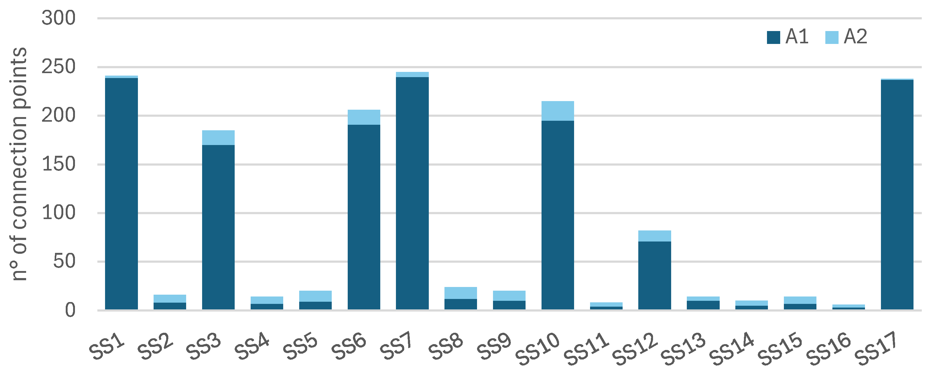
The dataset includes substations with markedly different sizes and user compositions, ranging from small SSs with only a few connection points to larger ones supplying more than 200 connection points. Moreover, the relative presence of consumption and production connection points varies considerably across the analyzed SSs, providing a heterogeneous set of operating conditions for the subsequent forecasting analysis.
3.2. Secondary Substation Classification
Applying the energy-ratio criterion defined in Eq.(2) to the 17 secondary substations reveals markedly different operating conditions across the analyzed distribution area. Figure 4 shows, for each substation, the annual consumed energy (A1), produced energy (A2), their ratio , and the resulting operating class.
Overall, the analysis distinguishes consumption-dominated passive substations, generation-dominated active substations, and intermediate hybrid cases where both consumption and local generation contribute significantly to the annual energy balance. These differences are also reflected in the measured power profiles. As shown by the representative examples in Figure 5, passive substations exhibit a regular and recurrent daily pattern in withdrawn power (A1), whereas injected power (A2) is shown for hybrid and active substations. Hybrid substations display a recognizable daily generation pattern, concentrated during daylight hours and characterized by a bell-shaped profile, consistent with a predominant photovoltaic contribution. Conversely, active substations exhibit more irregular generation, with large variations throughout the day and no clearly repeatable daily pattern, consistent with the predominance of wind generation. The temporal profiles therefore complement the annual energy balance by revealing distinct operating patterns across the three classes. These differences are further confirmed by the corresponding autocorrelation functions. Passive substations exhibit pronounced ACF peaks at approximately 24 h and its multiples, reflecting the strong daily periodicity of consumption. A similarly clear structure is observed for hybrid substations, where photovoltaic generation produces recurring daily peaks. In contrast, active substations show a much weaker autocorrelation structure, with a rapid decay and limited periodicity at longer lags, reflecting the greater variability of wind generation.
The classification therefore captures not only different balances between consumption and generation, but also distinct temporal structures that directly affect forecasting. The strong autocorrelation of passive and photovoltaic-dominated hybrid substations provides useful information for autoregressive forecasting, whereas wind-dominated active substations are less predictable from historical power measurements alone. These differences provide a physical and statistical basis for interpreting the forecasting performance of the three classes in the following analysis.
3.3. Short-Term Load Forecasting
Forecasting performance is analyzed separately for passive, hybrid, and active substations to highlight the differences associated with their operating characteristics.
3.3.1. Passive Substations
Passive substations represent the conventional load forecasting case, as their power exchange is predominantly determined by the consumption of the underlying connection points. Their profiles exhibit regular daily and weekly patterns, providing a strong temporal structure that can be exploited by the autoregressive and calendar features of the forecasting framework.
Figure 6 shows an example for SS1 over five days of the validation period. The five horizon-specific models reproduce the main evolution of the measured load, including the overnight minimum, the morning increase, and the daily load cycles. Differences among the forecasts become more evident during the periods of rapid load variation and around the daily peaks. The lower panel confirms that the largest errors occur mainly during these high load periods, whereas the forecasts remain closer to the measurements during the more stable overnight conditions.
Table 3 extends the analysis to all passive substations and reports both MAE and MAPE for the five forecasting horizons. At D-1, the MAE ranges from 4.34 kW for SS3 to 8.01 kW for SS7, while the MAPE remains between 6.95% and 14.41%. The performance progressively deteriorates as the forecast horizon increases. At D-5, the MAE ranges from 4.83 to 11.94 kW and the MAPE from 9.70% to 15.35%. This trend is observed across all six passive substations.
Overall, the results indicate that the proposed approach provides consistent short-term forecasts for passive substations, while confirming the expected loss of accuracy as the available historical information becomes more distant from the target day. The relatively gradual degradation from D-1 to D-5 suggests that the recurring daily and weekly structure of passive demand remains informative even at longer forecasting horizons.
3.3.2. Hybrid Substations
Hybrid substations are characterized by significant contributions from both consumption (A1) and local generation (A2), which are therefore forecast separately.
Figure 7 shows the validation results for SS12 over five representative days. For A1, the five horizon-specific models reproduce the main load pattern, with the largest errors occurring around daily peaks and sharp variations. For A2, the models correctly capture the photovoltaic generation windows but show larger discrepancies in peak magnitude. In particular, the measured peaks vary considerably from day to day, while the forecasts tend to reproduce a more regular generation pattern.
Table 4 extends the analysis to both hybrid substations and reports the MAE and MAPE for A1 and A2 across the five forecasting horizons.
For A1, the D-1 MAE is 6.75 kW for SS12 and 10.39 kW for SS13, with corresponding MAPE values of 19.06% and 22.09%. Accuracy progressively decreases toward D-5, where the MAE reaches 8.15 kW and 11.40 kW, respectively. Compared with passive substations, the withdrawal forecast therefore exhibits higher relative errors, while maintaining a similar gradual degradation with the forecasting horizon.
For A2, the absolute errors are considerably smaller, with D-1 MAE values of 2.05 kW for SS12 and 1.31 kW for SS13. However, the corresponding MAPE values are much higher, ranging from 53.61% to 69.12% at D-1 and reaching up to 98.09% at D-5.
Overall, the results show that the forecasting framework retains good capability in reproducing the temporal evolution of withdrawn power in hybrid substations, although with higher errors than in the passive case. The injected power forecast captures the occurrence and timing of the daily generation periods, but reproducing their amplitude is more challenging. The distinction between A1 and A2 therefore highlights the different forecasting behavior of the consumption and generation-related components within the same operating class.
3.3.3. Active Substations
Active substations represent the most challenging forecasting case due to the highly variable behaviour of their injected power (A2).
Figure 8 shows the validation results for SS2 over five representative days. The five horizon-specific models capture the general evolution of A2 and the main periods of high and low generation but show larger discrepancies during rapid variations and transitions between operating levels. In particular, the forecasts tend to smooth the measured profile, failing to fully reproduce the magnitude and timing of short-term fluctuations. Consequently, the largest errors occur during the most abrupt changes in injected power.
Table 5 extends the analysis to all active substations and reports the MAE and MAPE across the five forecasting horizons.
At D-1, the MAE varies considerably across the class, from 3.36 kW for SS16 to 39.82 kW for SS8, while the MAPE ranges from 62.97% to 87.51%. Unlike the passive and hybrid cases, however, increasing the forecasting horizon does not result in a systematic degradation of performance. For several substations, the MAE and MAPE remain nearly unchanged from D-1 to D-5, while in some cases they even decrease slightly.
Overall, the results indicate that injected power forecasting in active substations is substantially more challenging than load forecasting in passive substations. More importantly, the limited variation in accuracy across D-1 to D-5 suggests that reducing the forecasting horizon provides only a modest advantage for these profiles. The dominant limitation is therefore not the progressive loss of recent historical information with increasing horizon, but the difficulty of reproducing the short-term variability of the generation profile from the information available to the forecasting model. This is particularly relevant for the active substations considered here, whose injected power is predominantly associated with wind generation. Accurate wind power forecasting generally requires dedicated forecasting approaches combining meteorological information with plant-specific characteristics, such as wind conditions at hub height, turbine technology and power curves, and other operational data [28]. The absence of this information limits the ability of the present general-purpose framework to reproduce the highly variable generation profiles observed in this class.
3.4. Forecasting Drivers
The differences in forecasting performance across the operating classes can be interpreted by examining the information exploited by the trained models. To this purpose, the RF feature importance is grouped into three families: autoregressive, weather, and calendar variables. Figure 9 reports the relative contribution of each family for the relevant combinations of operating class and power-flow direction.
A clear distinction emerges between consumption and generation forecasting. For A1, autoregressive features dominate in both passive and hybrid substations, accounting for 89% and 78% of the total importance, respectively. This is consistent with the regular temporal structure of consumption observed in these classes. For hybrid A2, the autoregressive contribution decreases to 69%, while meteorological variables increase to 20%, reflecting the greater influence of weather conditions on the predominantly photovoltaic generation. A markedly different distribution is observed for active substations. For A2, meteorological variables become dominant, accounting for 74% of the total importance, while the autoregressive contribution drops to 15%. This is consistent with the predominantly wind-driven generation of this class, whose evolution is more strongly influenced by meteorological conditions than by past power measurements.
These results also help explain the differences observed across forecasting horizons. The strong autoregressive contribution in passive and hybrid substations is consistent with the progressive loss of accuracy from D-1 to D-5, as recent historical information becomes less accessible at longer horizons. Conversely, the limited role of autoregressive features in active substations is consistent with the smaller performance differences across horizons, as their forecasts rely primarily on meteorological information.
3.5. Hierarchical Reconciliation
The reconciliation results are analyzed separately for the three operating classes, as its effectiveness depends on the composition of the underlying hierarchy. Figure 10 shows the distribution of connection points across the three contractual power clusters for each substation. Passive substations generally include a large number of connection points distributed across multiple clusters, allowing individual behavior to be averaged within each aggregate. For instance, SS1 includes 139 points below 3.3 kW and 76 between 3.3 and 6.6 kW, compared with only 3 above 6.6 kW. In contrast, active substations concentrate their injection in the largest power cluster, typically comprising only 1 to 6 connection points. Their hierarchy therefore consists of a few large generators, providing little aggregation compared with passive substations.
Figure 11 shows the four lower-level nodes of the hierarchy for SS1 over a representative five-day period. Their forecasting performance varies considerably across nodes. The two smaller contractual clusters, which aggregate a larger number of connection points, achieve R2 values of 0.84 and 0.85, whereas the largest-power cluster, composed of fewer and more irregular connection points, reaches only 0.40. The error index also exhibits a recurring daily pattern and is forecast with an R2 of 0.64. These differences are relevant for reconciliation, as the effectiveness of the MinT projection depends on the predictive information provided by the lower-level forecasts.
3.5.1. Passive Substations
Passive substations provide favorable conditions for hierarchical reconciliation, as their connection point aggregates retain the regular temporal structure of the substation load. Figure 12 compares the base (RF) and reconciled (RF+MinT) day-ahead forecasts for SS1. Both closely reproduce the measured load profile, with the largest deviations occurring around the sharpest peaks. Reconciliation mainly reduces local forecast errors rather than altering the overall profile, with the RF+MinT errors generally confined to a narrower range and fewer pronounced deviations. MinT therefore provides a targeted correction of the base forecast while preserving its overall temporal evolution.
Table 6 extends the comparison to all passive substations. Reconciliation reduces the MAE on 6 of the 6 substations, with a median change of -3.4% and a largest change of -6.4%, and it improves the MAPE on the same cases, with a median change of -0.33 percentage points. The improvement is consistent across the class and both metrics, although moderate in magnitude, indicating that reconciliation primarily corrects local deviations while preserving the overall forecast profile.
3.5.2. Hybrid Substations
In hybrid substations, reconciliation is performed separately for the two power-flow directions, allowing its impact on A1 and A2 forecasting to be assessed independently. Figure 13 compares the base and reconciled forecasts of SS12 for both power-flow directions. For A1, reconciliation introduces moderate corrections throughout the profile, with the largest differences occurring around daily peaks and rapid load variations. For A2, the effect is more localized but also more pronounced, with MinT mainly modifying the magnitude of the daily generation peaks. These corrections do not systematically bring the forecast closer to the measured profile, indicating that the effectiveness of reconciliation differs between the two power-flow directions.
Table 7 reports the reconciliation results for both targets of the two hybrid substations. For A1, the median MAE decreases by 0.99%, indicating a smaller and less consistent improvement than for passive substations. For A2, the median MAE increases slightly by 1.49%, while MAPE decreases by 0.54 percentage points. Overall, reconciliation therefore provides limited benefits for hybrid substations, with its impact depending on both the considered target and performance metric.
3.5.3. Active Substations
For active substations the analysis is restricted to the injected power. Figure 14 shows that the base and reconciled forecasts of SS2 are nearly coincident over the whole window, and that their error traces are almost identical. The limited benefit of reconciliation is consistent with the low predictability of the lower-level nodes, which provides MinT with less informative error structures to exploit.
Table 8 confirms this across the class. The median change in MAE is -0.20%, with improvements on 5 of the 9 substations only, and the individual values vary around zero, ranging from -0.5% to +7.9%. The median change in MAPE is negligible, at +0.05 percentage points. Enforcing coherence on this class therefore neither helps nor harms the accuracy of the substation forecast in any systematic way.
Reconciliation also entails an additional computational cost, which is the same for every class. The hierarchical framework requires one model for each connection-point cluster, together with separate models for the error index and the substation, resulting in a higher computational cost than the base forecast. Most of this additional cost is associated with training the lower-level forecasting models, while the MinT projection itself introduces only a limited computational overhead. While acceptable for an individual substation, this overhead becomes significant when the procedure is extended across a large population, two flow directions and five forecasting horizons.
Overall, the results show that the main benefit of hierarchical reconciliation is the enforcement of coherence across aggregation levels, while improvements in forecasting accuracy depend on the quality of the lower-level forecasts. For passive substations, where connection-point aggregates are based on a large number of customers and retain regular temporal patterns, MinT provides a consistent, although moderate, improvement across the entire class. The benefit becomes less systematic for hybrid substations and is negligible for active substations, where the lower-level nodes consist of fewer and more variable generators. These results indicate that the effectiveness of reconciliation is closely related to the predictability of the underlying hierarchy. MinT therefore guarantees coherent forecasts in all cases, while its contribution to forecasting accuracy is greatest when the lower-level aggregates provide reliable predictive information.
4. Conclusions
This paper presented a data-driven framework for short-term forecasting at SS level, combining the characterization of substation operating conditions, horizon specific RF models, and hierarchical reconciliation through the MinT method. The methodology was assessed on one year of quarter-hourly measurements from 17 secondary substations and their underlying connection points, considering withdrawn (A1) and injected (A2) power separately.
The results show that the operating characteristics of a substation strongly affect its forecasting performance. Passive substations exhibit regular and highly autocorrelated consumption profiles, resulting in accurate forecasts and a gradual loss of performance from D-1 to D-5. Hybrid substations retain similar characteristics for withdrawn power, while their predominantly photovoltaic injection introduces greater variability, particularly in the magnitude of generation peaks. Active substations represent the most challenging case. Their predominantly wind-driven injection exhibits weaker temporal persistence and substantially higher forecasting errors, with comparatively limited differences across forecasting horizons. This indicates that increasing the availability of recent historical measurements alone is insufficient to improve forecasts for highly variable generation profiles.
The feature-importance analysis supports this interpretation. Autoregressive information dominates withdrawn-power forecasting for passive and hybrid substations, accounting for 89% and 78% of the total importance, respectively, and remains relevant for photovoltaic-dominated hybrid injection at 69%. Conversely, meteorological variables account for 74% of the importance for active-substation injection, while the autoregressive contribution decreases to 15%. These results show that the most relevant forecasting information varies with the operating characteristics of the substation, supporting the use of differentiated forecasting approaches across the analyzed classes.
Hierarchical reconciliation exhibits a similar dependence on the characteristics of the underlying hierarchy. MinT guarantees coherence between substation and lower level forecasts in all cases, but its contribution to forecasting accuracy depends on the predictability of the connection point aggregates. For passive substations, where clusters aggregate many connection points with regular consumption patterns, reconciliation consistently improves the day-ahead forecast, reducing MAE for all six substations with a median improvement of 3.4%. Its benefit becomes less systematic for hybrid substations and negligible for active substations, whose lower-level hierarchy consists of fewer and more variable generation units. Thus, while coherence is ensured independently of forecasting accuracy, the accuracy benefit of reconciliation is greatest when reliable information is available at the lower levels of the hierarchy.
Overall, the study shows that forecasting performance at SS level cannot be considered independently of the operating characteristics of the underlying network. The proposed classification provides a simple means of identifying different forecasting conditions and interpreting the expected performance of both the base and reconciled forecasts. From a DSO perspective, this supports a differentiated forecasting strategy in which conventional autoregressive approaches remain effective for consumption dominated substations, while generation dominated substations require more specialized models and information. Future work should therefore focus on generation aware forecasting approaches incorporating more detailed meteorological forecasts and plant specific information, particularly for wind dominated substations, together with scalable reconciliation strategies suitable for deployment across large substation populations.
Author Contributions
Conceptualization, D.A., M.S., G.R. and M.M.; methodology, D.A., M.S., G.R. and M.M.; software, D.A. and M.S.; validation, D.A., M.S., G.R. and M.M.; formal analysis, M.S. and M.M.; investigation, D.A. and M.S.; resources, G.R. and M.M.; data curation, D.A. and M.S.; writing—original draft preparation, D.A.; writing—review and editing, M.S., G.R. and M.M.; visualization, D.A. and M.S.; supervision, G.R. and M.M.; project administration, G.R. and M.M.; funding acquisition, G.R. and M.M. All authors have read and agreed to the published version of the manuscript.
Funding
This work was supported by the G.E.M.I.N.I. project, funded by the Italian Ministry of Environment and Energy Security (MASE) under Mission Innovation 2.0 – Green Powered Future Mission (GPFM), pursuant to Ministerial Decree No. 386 of 17 November 2023.
Data Availability Statement
The datasets presented in this article are not publicly available because they contain sensitive information and were provided to the authors under confidentiality restrictions that prohibit their disclosure.
Conflicts of Interest
The authors declare no conflicts of interest.
References
- EU Market Outlook for Solar Power 2024-2028 - SolarPower Europe. Available online: https://www.solarpowereurope.org/insights/outlooks/eu-market-outlook-for-solar-power-2024-2028/detail (accessed on Aug. 13 2026).
- Number of EVs, air conditioners, and heat pumps in operation in the Stated Policies Scenario, 2023 and 2035 – Charts – Data & Statistics - IEA. Available online: https://www.iea.org/data-and-statistics/charts/number-of-evs-air-conditioners-and-heat-pumps-in-operation-in-the-stated-policies-scenario-2023-and-2035 (accessed on Aug. 13 2026).
- Kotsonias; Hadjidemetriou, L.; Asprou, M.; Panayiotou, C. G. Operational challenges and solution approaches for low voltage distribution grids — A review. Electr. Power Syst. Res. 2025, vol. 239, 111258. [Google Scholar] [CrossRef]
- Scrocca, et al. Local flexibility markets in Europe: A critical review of market designs, operational maturity and stakeholder perspectives. Renew. Sustain. Energy Rev. 2026, vol. 226, 116434. [Google Scholar] [CrossRef]
- Wang, Y.; Zhang, N.; Chen, Q.; Kirschen, D. S.; Li, P.; Xia, Q. Data-Driven Probabilistic Net Load Forecasting With High Penetration of Behind-the-Meter PV. IEEE Trans. Power Syst. 2018, vol. 33(no. 3), 3255–3264. [Google Scholar] [CrossRef]
- Dorostkar-Ghamsari, M. R.; Fotuhi-Firuzabad, M.; Lehtonen, M.; Safdarian, A.; Hoshyarzade, A. S. Stochastic Operation Framework for Distribution Networks Hosting High Wind Penetrations. IEEE Trans. Sustain. Energy 2019, vol. 10(no. 1), 344–354. [Google Scholar] [CrossRef]
- Lusis, P.; Khalilpour, K. R.; Andrew, L.; Liebman, A. Short-term residential load forecasting: Impact of calendar effects and forecast granularity. Appl. Energy 2017, vol. 205, 654–669. [Google Scholar] [CrossRef]
- Khan, Z. A.; et al. Efficient Short-Term Electricity Load Forecasting for Effective Energy Management. Sustain. Energy Technol. Assess. 2022, vol. 53, 102337. [Google Scholar] [CrossRef]
- Sun, X.; et al. An Efficient Approach to Short-Term Load Forecasting at the Distribution Level. IEEE Trans. Power Syst. 2016, vol. 31(no. 4), 2526–2537. [Google Scholar] [CrossRef]
- Rouwhorst, G.; Duque, E. M. S.; Nguyen, P. H.; Slootweg, H. Improving Clustering-Based Forecasting of Aggregated Distribution Transformer Loadings with Gradient Boosting and Feature Selection. IEEE Access 2022, vol. 10, 443–455. [Google Scholar] [CrossRef]
- Ding, N.; Benoit, C.; Foggia, G.; Besanger, Y.; Wurtz, F. Neural network-based model design for short-term load forecast in distribution systems. IEEE Trans. Power Syst. 2016, vol. 31(no. 1), 72–81. [Google Scholar] [CrossRef]
- Kong, W.; Dong, Z. Y.; Jia, Y.; Hill, D. J.; Xu, Y.; Zhang, Y. Short-Term Residential Load Forecasting Based on LSTM Recurrent Neural Network. IEEE Trans. Smart Grid 2019, vol. 10(no. 1), 841–851. [Google Scholar] [CrossRef]
- Grabner, M.; Wang, Y.; Wen, Q.; Blazic, B.; Struc, V. A Global Modeling Framework for Load Forecasting in Distribution Networks. IEEE Trans. Smart Grid 2023, vol. 14(no. 6), 4927–4941. [Google Scholar] [CrossRef]
- Faustine; Nunes, N. J.; Pereira, L. Efficiency Through Simplicity: MLP-Based Approach for Net-Load Forecasting With Uncertainty Estimates in Low-Voltage Distribution Networks. IEEE Trans. Power Syst. 2025, vol. 40(no. 1), 46–56. [Google Scholar] [CrossRef]
- Caballero-Peña, J.; Cadena-Zarate, C.; Parrado-Duque, A.; Osma-Pinto, G. Distributed energy resources on distribution networks: A systematic review of modelling, simulation, metrics, and impacts. Int. J. Electr. Power Energy Syst. 2022, vol. 138, 107900. [Google Scholar] [CrossRef]
- Wilms, H.; Cupelli, M.; Monti, A. On the Necessity of Exogenous Variables for Load, PV and Wind Day-Ahead Forecasts using Recurrent Neural Networks. 2018 IEEE Electrical Power and Energy Conference, EPEC 2018, Dec. 2018. [Google Scholar] [CrossRef]
- Hayes, P.; Gruber, J. K.; Prodanovic, M. Multi-nodal short-term energy forecasting using smart meter data. In IET Generation, Transmission and Distribution; WEBSITE:WEBSITE:IET-SITE; STRING:PUBLICATION: WGROUP, Jul 2018; vol. 12, no. 12, pp. 2988–2994. [Google Scholar] [CrossRef]
- Shering, T.; Alonso, E.; Apostolopoulou, D. Investigation of Load, Solar and Wind Generation as Target Variables in LSTM Time Series Forecasting, Using Exogenous Weather Variables. Energies 2024, Vol. 17, vol. 17(no. 8). [Google Scholar] [CrossRef]
- Wang, J.; Zhong, H.; Lai, X.; Xia, Q.; Wang, Y.; Kang, C. Exploring key weather factors from analytical modeling toward improved solar power forecasting. IEEE Trans. Smart Grid 2019, vol. 10(no. 2), 1417–1427. [Google Scholar] [CrossRef]
- Pinheiro, M. G.; Madeira, S. C.; Francisco, A. P. Short-term electricity load forecasting—A systematic approach from system level to secondary substations. Appl. Energy 2023, vol. 332, 120493. [Google Scholar] [CrossRef]
- Nespoli, L.; Medici, V.; Lopatichki, K.; Sossan, F. Hierarchical demand forecasting benchmark for the distribution grid. Electr. Power Syst. Res. 2020, vol. 189, 106755. [Google Scholar] [CrossRef]
- Wickramasuriya, S. L.; Athanasopoulos, G.; Hyndman, R. J. Optimal Forecast Reconciliation for Hierarchical and Grouped Time Series Through Trace Minimization. J. Am. Stat. Assoc. 2019, vol. 114(no. 526), 804–819. [Google Scholar] [CrossRef]
- Mogos, S.; Ansari, O. A.; Liang, X.; Chung, C. Y. Hierarchical Load Forecast Aggregation for Distribution Transformers Using Minimum Trace Optimal Reconciliation and AMI Data. IEEE Access 2023, vol. 11, 93472–93486. [Google Scholar] [CrossRef]
- Bao, Y.; Xiong, T.; Hu, Z. Multi-step-ahead time series prediction using multiple-output support vector regression. Neurocomputing 2014, vol. 129, 482–493. [Google Scholar] [CrossRef]
- Free Open-Source Weather API | Open-Meteo.com. Available online: https://open-meteo.com/ (accessed on Aug. 14 2026).
- Breiman, L. “Random forests,”. Mach. Learn. 2001, vol. 45(no. 1), 5–32. [Google Scholar] [CrossRef]
- Cerqueira, V.; Torgo, L.; Mozetič, I.; Soldatova, L.; Vanschoren, J.; Mozetič igormozetic, I. Evaluating time series forecasting models: an empirical study on performance estimation methods. Mach. Learn. 2020 109 11 2020, vol. 109(no. 11), 1997–2028. [Google Scholar] [CrossRef]
- Hanifi, S.; Liu, X.; Lin, Z.; Lotfian, S. A Critical Review of Wind Power Forecasting Methods—Past, Present and Future. Energies 2020 2020, Vol. 13, vol. 13(no. 15). [Google Scholar] [CrossRef]
Figure 1.
Reference structure of the LV grids under investigation.
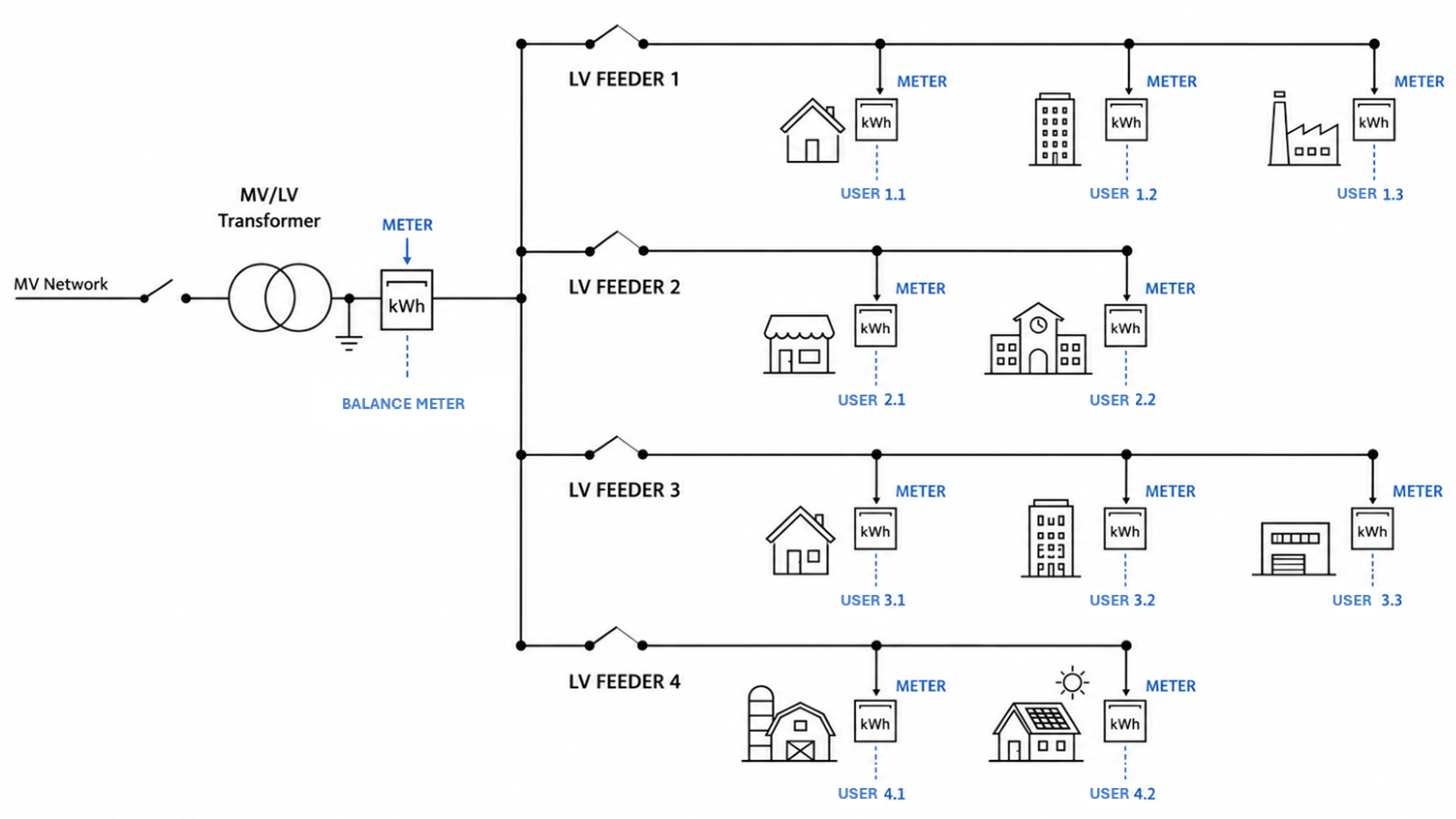
Figure 2.
Geographical distribution of the analysed secondary substations.
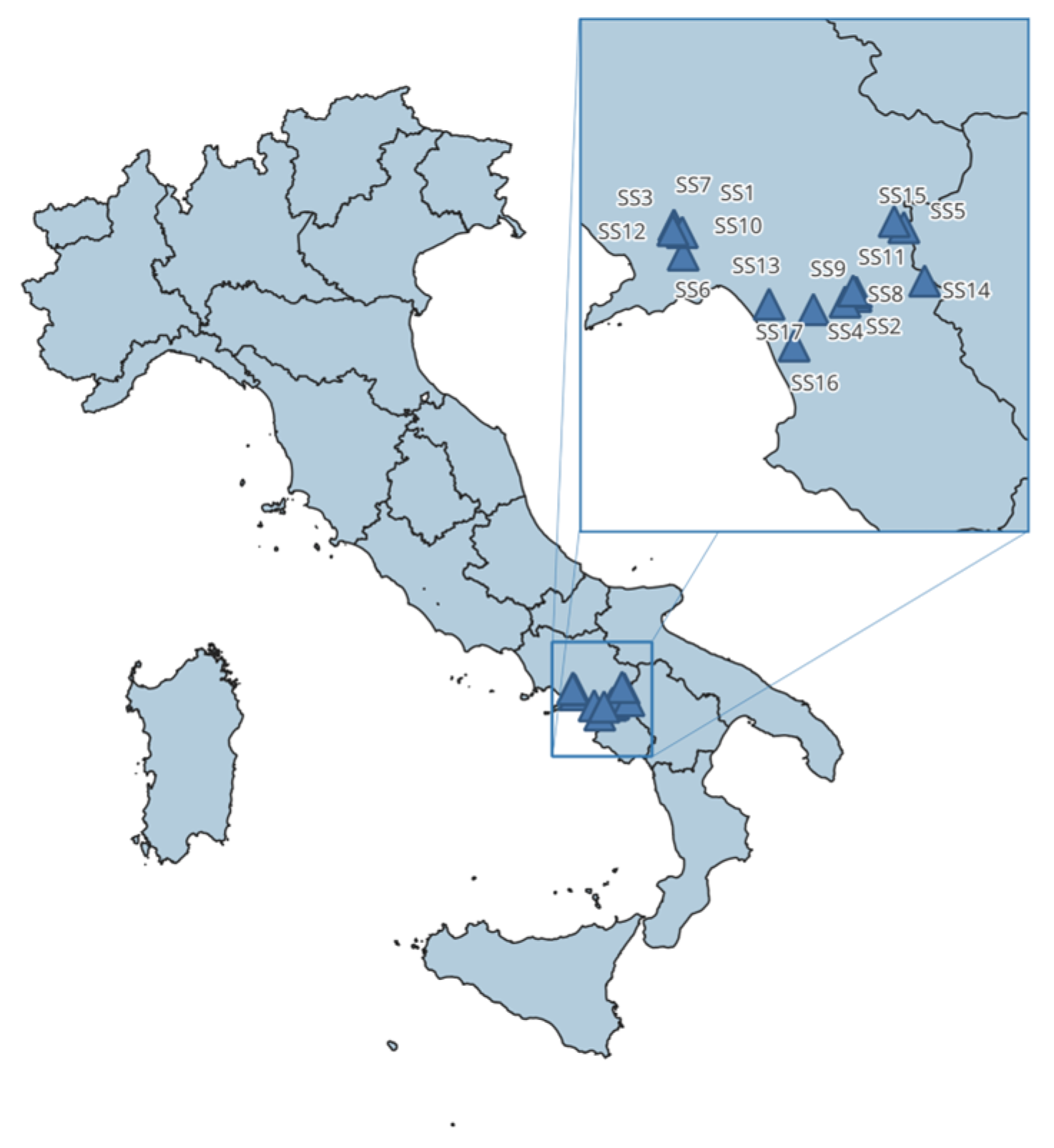
Figure 4.
Energy balance and operating classification of the analysed secondary substations.
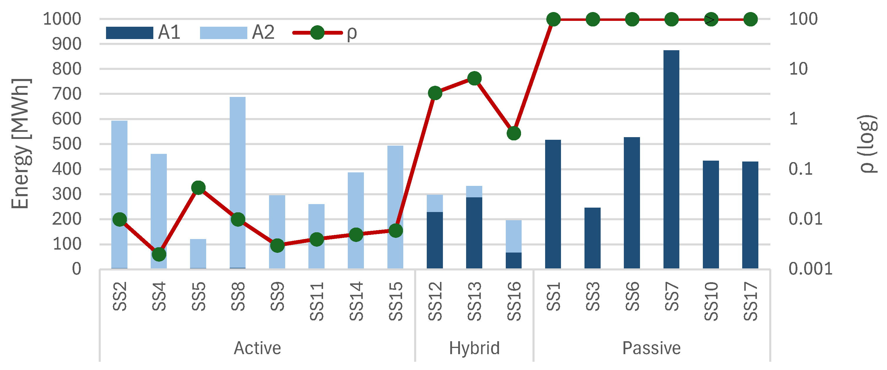
Figure 5.
Weekly power profiles with the corresponding ACF and PACF for (a) a passive (SS1), (b) a hybrid (SS16), and (c) an active (SS2) secondary substation.
Figure 5.
Weekly power profiles with the corresponding ACF and PACF for (a) a passive (SS1), (b) a hybrid (SS16), and (c) an active (SS2) secondary substation.
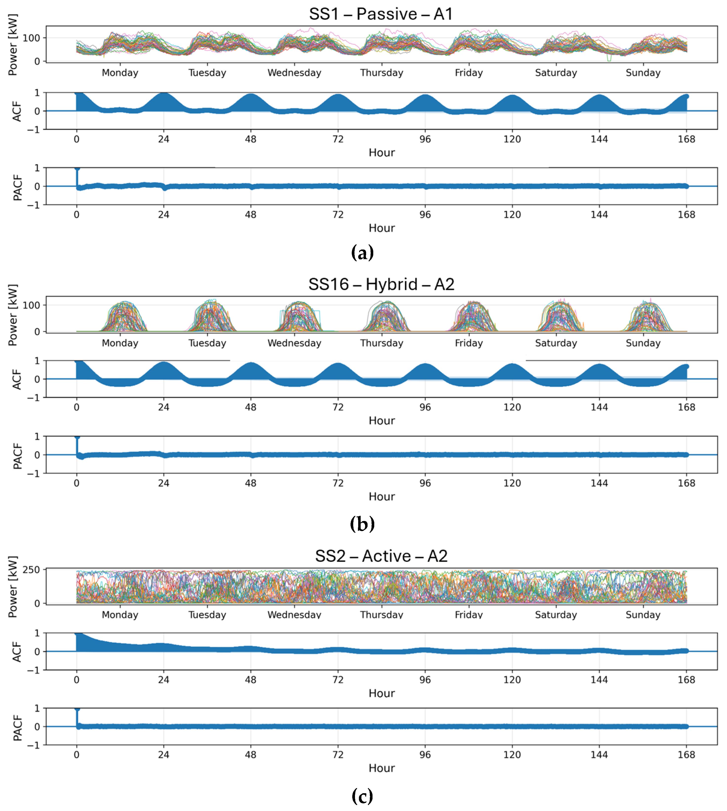
Figure 6.
Validation for the passive substation SS1: measured load (A1) and the five model predictions (top) and the corresponding errors (bottom).
Figure 6.
Validation for the passive substation SS1: measured load (A1) and the five model predictions (top) and the corresponding errors (bottom).
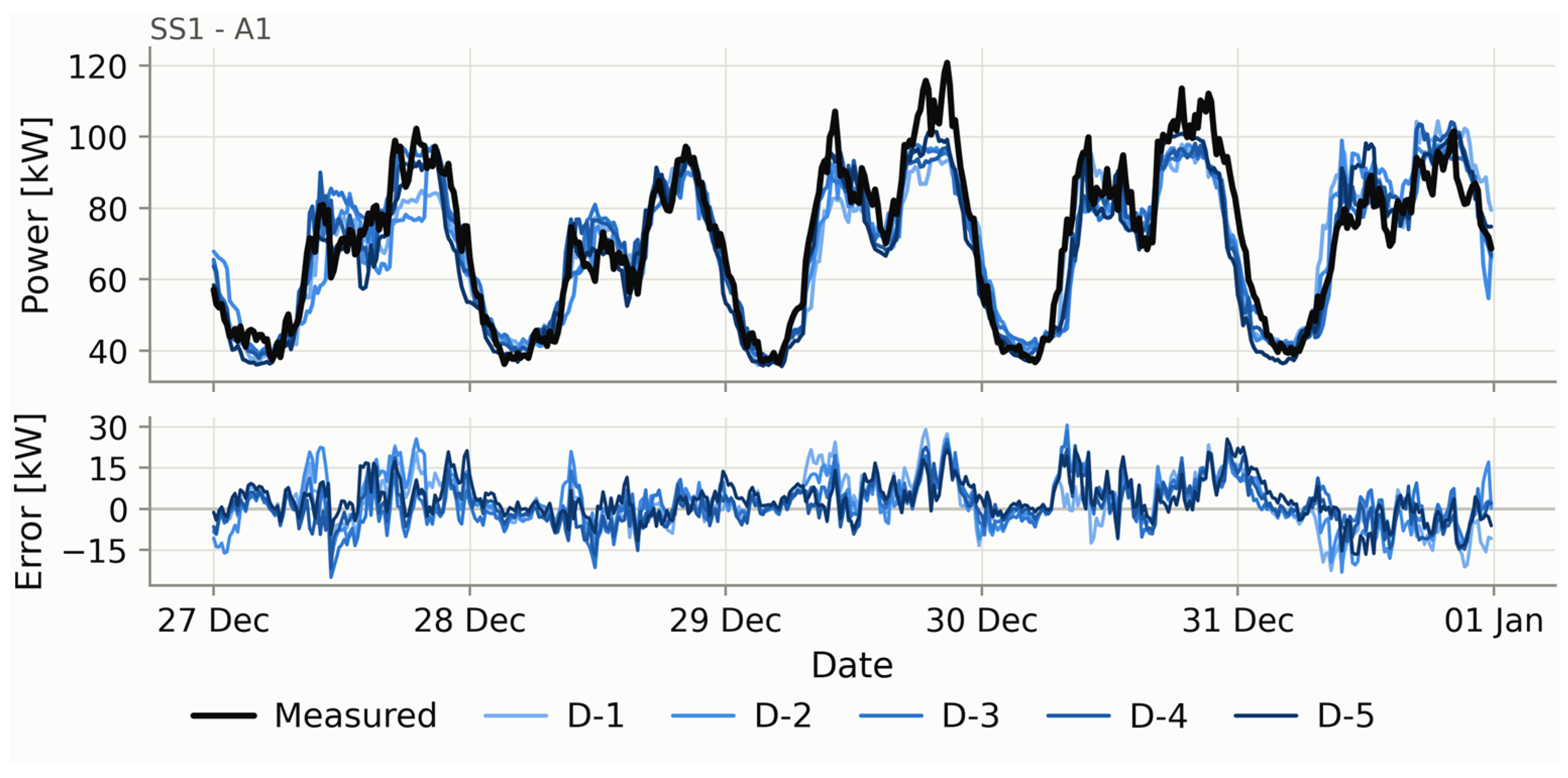
Figure 7.
Validation for the passive substation SS12: measured load (A1 and A2) and the five model predictions (top) and the corresponding errors (bottom).
Figure 7.
Validation for the passive substation SS12: measured load (A1 and A2) and the five model predictions (top) and the corresponding errors (bottom).
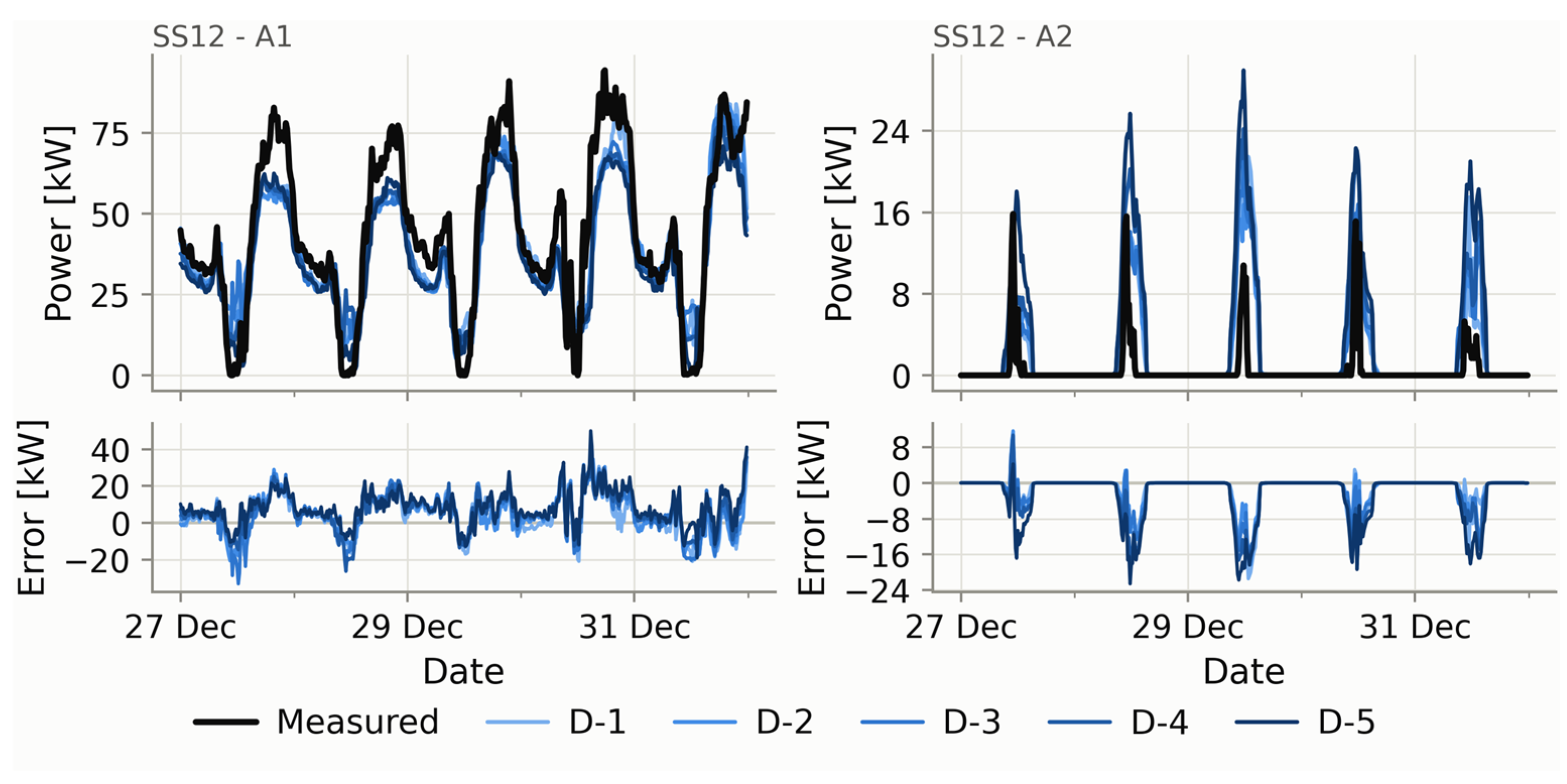
Figure 8.
Validation for the passive substation SS2: measured load (A2) and the five model predictions (top) and the corresponding errors (bottom).
Figure 8.
Validation for the passive substation SS2: measured load (A2) and the five model predictions (top) and the corresponding errors (bottom).
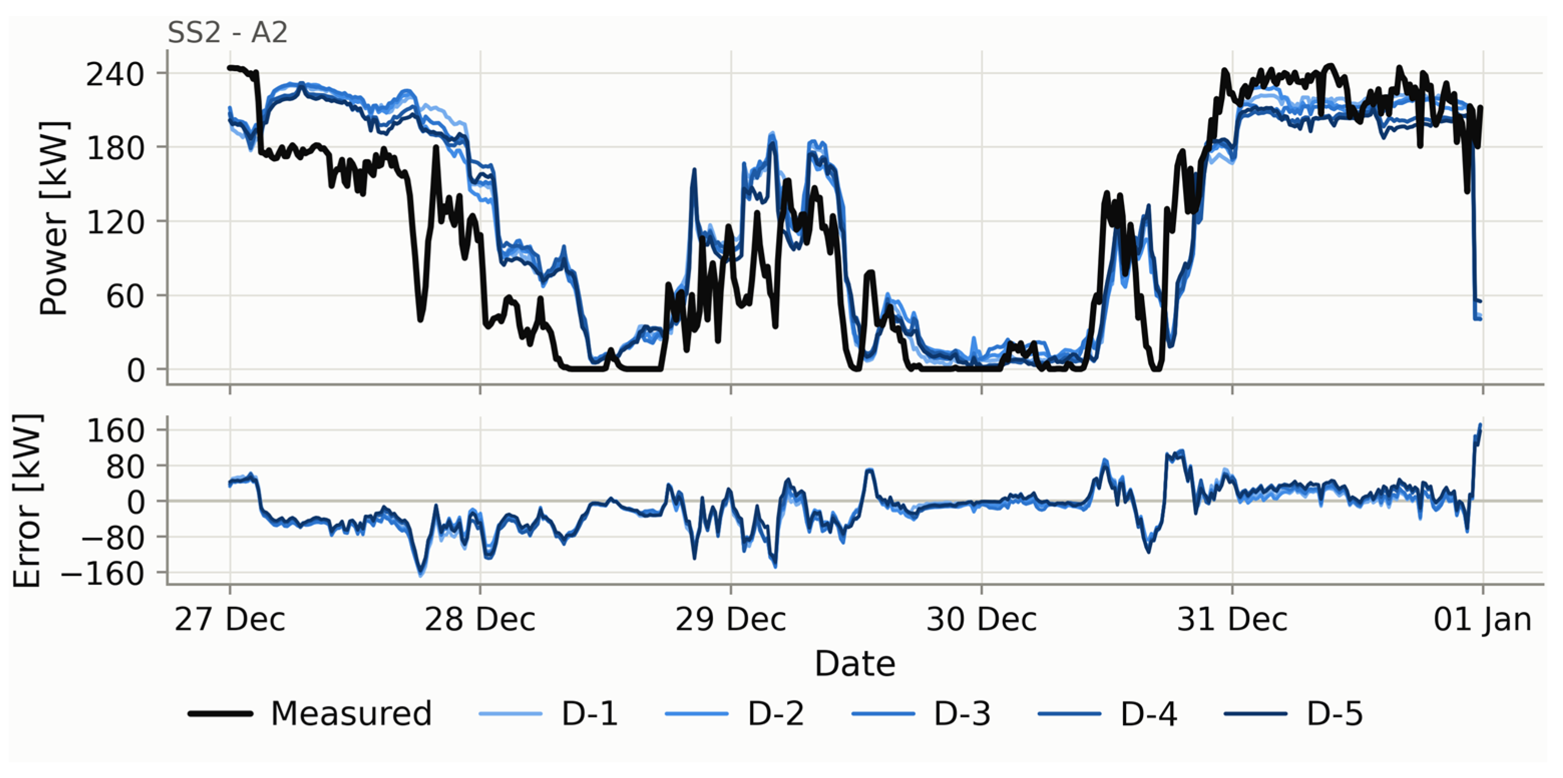
Figure 9.
Distribution of RF feature importance across the analyzed operating classes and power-flow directions.
Figure 9.
Distribution of RF feature importance across the analyzed operating classes and power-flow directions.
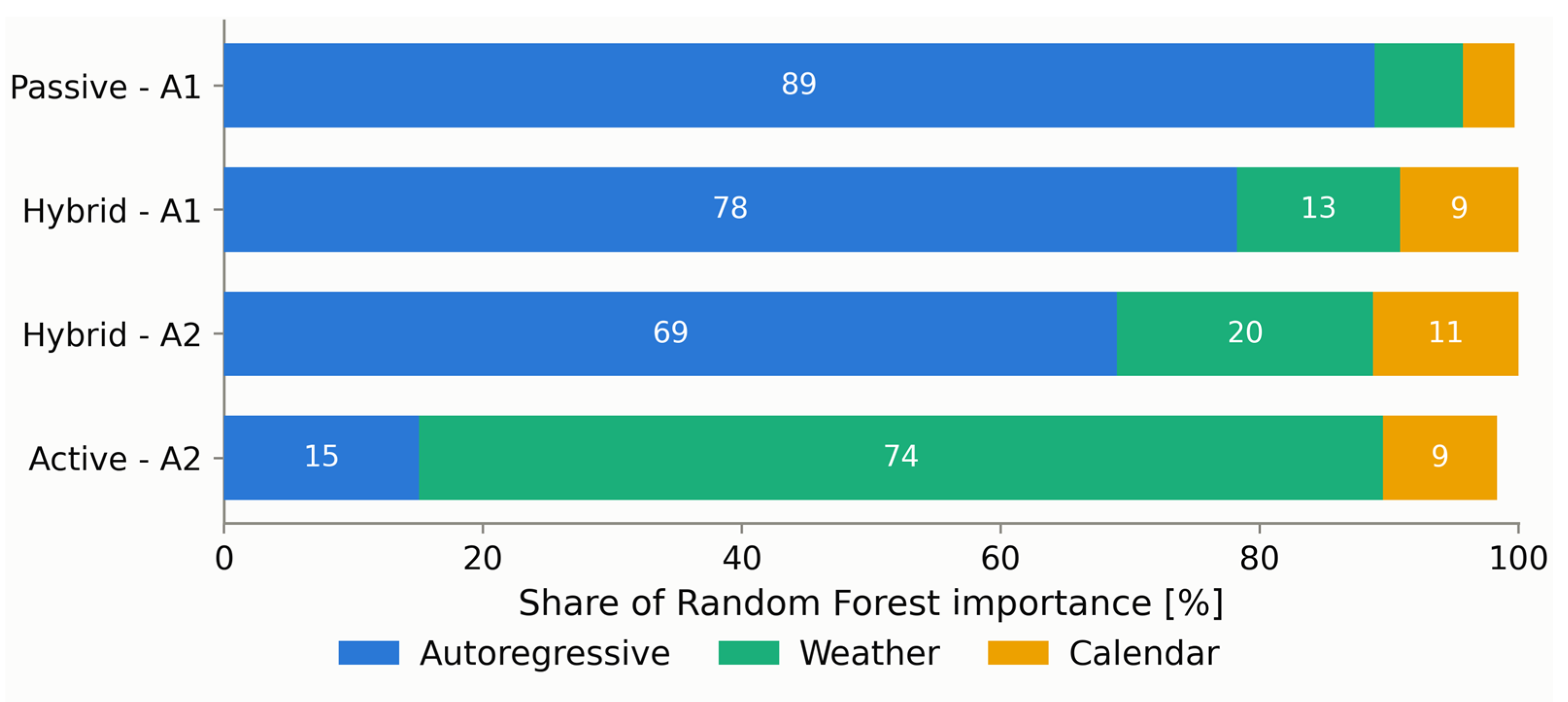
Figure 10.
Distribution of connection points among the three contractual-power clusters (<3.3 kW, 3.3–6.6 kW, and >6.6 kW) for each substation and odelled power-flow direction.
Figure 10.
Distribution of connection points among the three contractual-power clusters (<3.3 kW, 3.3–6.6 kW, and >6.6 kW) for each substation and odelled power-flow direction.
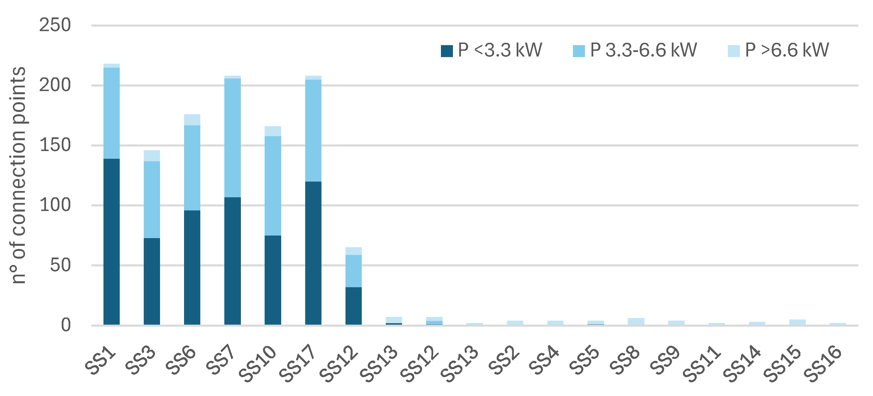
Figure 11.
Forecasting performance of the lower-level hierarchy for SS1 over the selected validation period.
Figure 11.
Forecasting performance of the lower-level hierarchy for SS1 over the selected validation period.
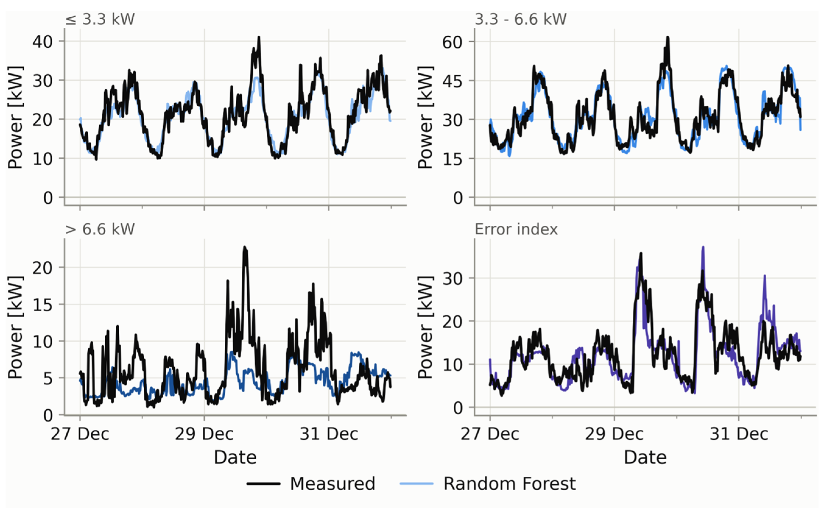
Figure 12.
Comparison of base and MinT day-ahead forecasts for passive substation SS1.
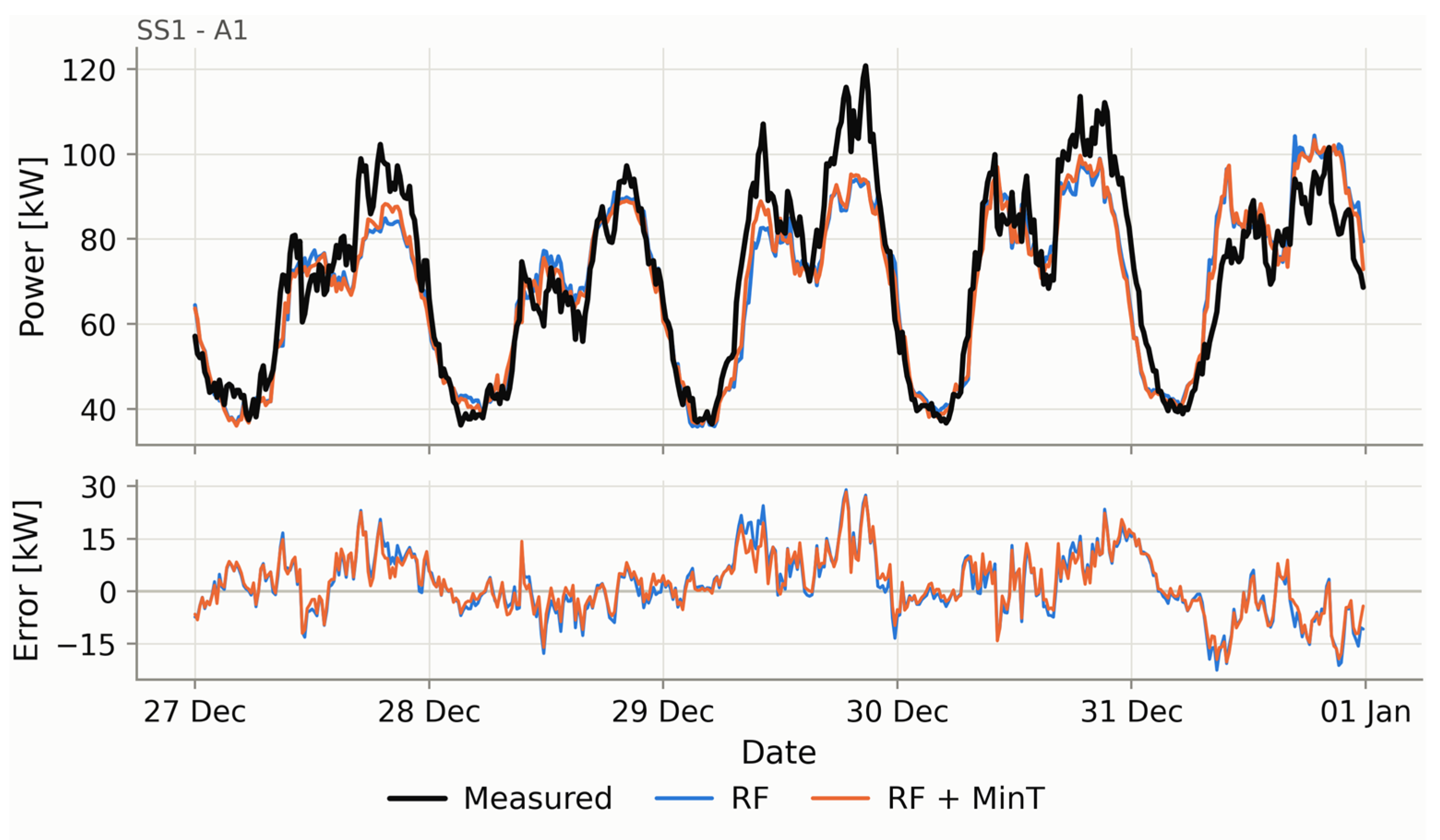
Figure 13.
Hybrid substation SS12: comparison of day-ahead base and MinT-reconciled forecasts for withdrawn power (A1) and injected power (A2), with corresponding errors.
Figure 13.
Hybrid substation SS12: comparison of day-ahead base and MinT-reconciled forecasts for withdrawn power (A1) and injected power (A2), with corresponding errors.
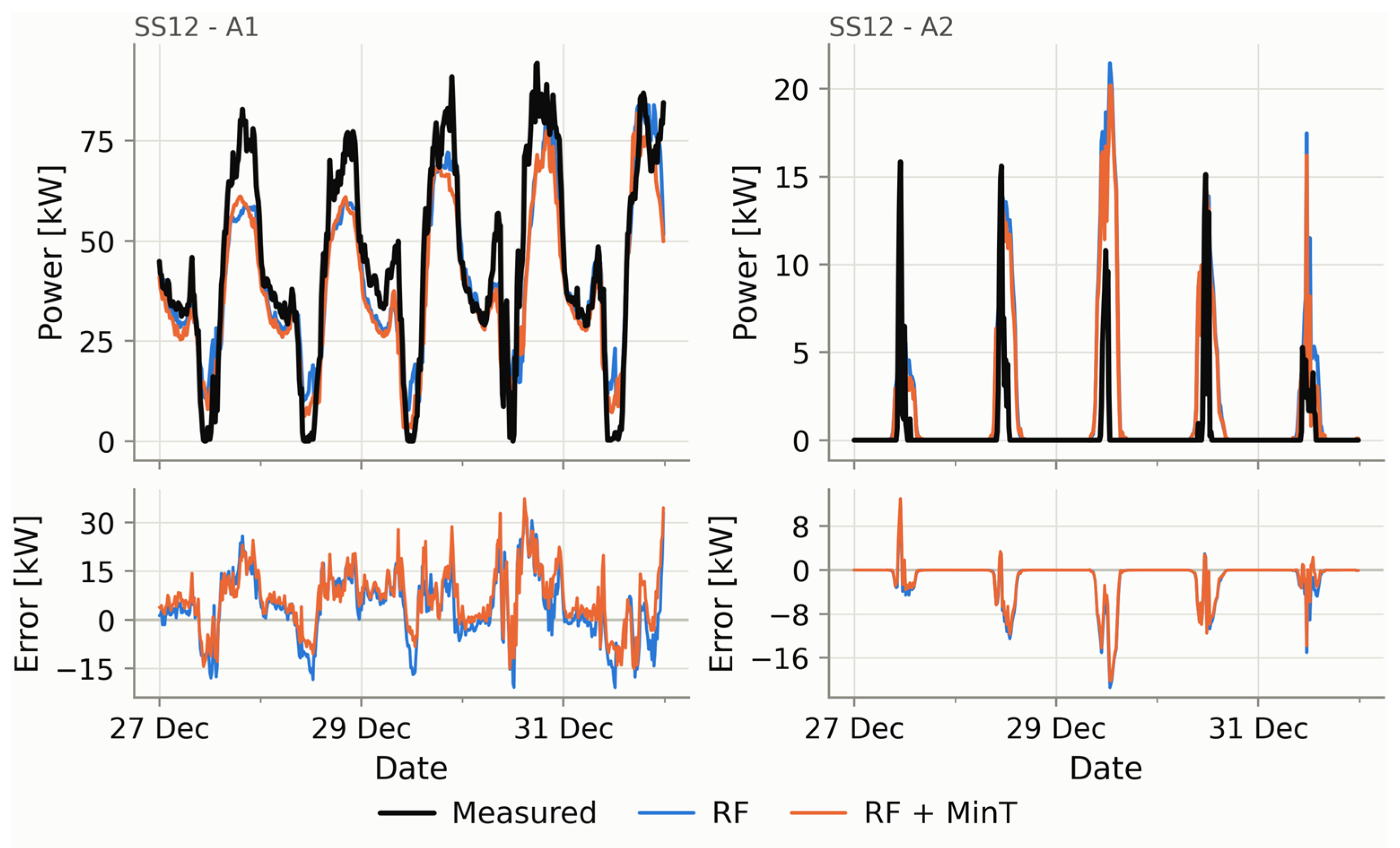
Figure 14.
Active substation SS2: comparison of the day-ahead base Random-Forest forecast and the MinT-reconciled forecast for injected power (A2), with corresponding errors.
Figure 14.
Active substation SS2: comparison of the day-ahead base Random-Forest forecast and the MinT-reconciled forecast for injected power (A2), with corresponding errors.
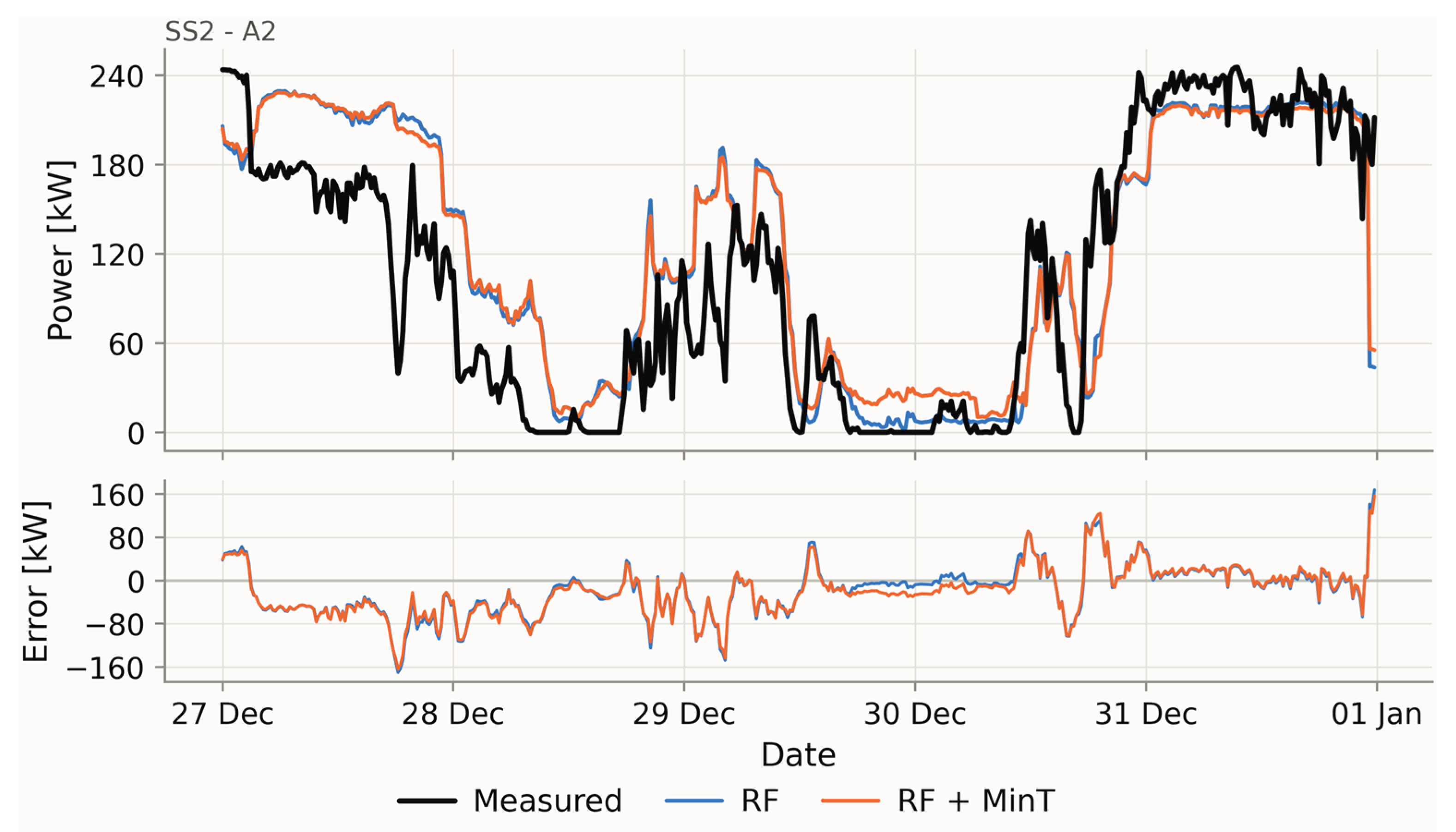

Table 1.
Autoregressive lags retained for each forecasting model.
| Model | Lag 1 | Lag 2 | Lag 3 | Lag 4 | Lag 5 |
|---|---|---|---|---|---|
|
RF1 (D-1) |
96 (1d) | 192 (2d) | 288 (3d) | 384 (4d) | 672 (1w) |
|
RF2 (D-2) |
192 (2d) | 288 (3d) | 384 (4d) | 480 (5d) | 672 (1w) |
|
RF3 (D-3) |
288 (3d) | 384 (4d) | 480 (5d) | 576 (6d) | 672 (1w) |
|
RF4 (D-4) |
384 (4d) | 480 (5d) | 576 (6d) | 672 (1w) | 1344 (2w) |
|
RF5 (D-5) |
480 (5d) | 576 (6d) | 672 (1w) | 1344 (2w) | 2016 (3w) |
Table 2.
Random Forest hyperparameter grid explored by the grid-search procedure.
| No. of trees | Max depth | Min samples/leaf | Max features |
|---|---|---|---|
| 200 | 10 | 1 | “sqrt” |
| 300 | 20 | 5 | 0.5 |
| 500 | 30 | 10 | 1 |
| - | None | - | - |
Table 3.
Validation MAE, MAPE, R2 of the 5 forecasting models (D-1 to D-5) for passive substations.
| Metric | D-1 | D-2 | D-3 | D-4 | D-5 | |
|---|---|---|---|---|---|---|
| SS1 | MAE [kW] | 5.833 | 6.077 | 6.211 | 6.703 | 7.864 |
| MAPE [%] | 8.71 | 9.00 | 9.28 | 10.01 | 11.48 | |
| R2 [-] | 0.869 | 0.862 | 0.855 | 0.832 | 0.767 | |
| SS3 | MAE [kW] | 4.340 | 4.511 | 4.407 | 4.614 | 4.834 |
| MAPE [%] | 14.41 | 14.94 | 14.56 | 14.76 | 15.35 | |
| R2 [-] | 0.766 | 0.743 | 0.753 | 0.717 | 0.689 | |
| SS6 | MAE [kW] | 6.626 | 7.070 | 7.096 | 7.411 | 8.406 |
| MAPE [%] | 9.04 | 9.50 | 9.50 | 9.82 | 11.00 | |
| R2 [-] | 0.809 | 0.782 | 0.783 | 0.765 | 0.712 | |
| SS7 | MAE [kW] | 8.013 | 8.710 | 9.181 | 10.336 | 11.940 |
| MAPE [%] | 6.95 | 7.49 | 7.85 | 8.67 | 9.77 | |
| R2 [-] | 0.902 | 0.880 | 0.869 | 0.833 | 0.781 | |
| SS10 | MAE [kW] | 6.900 | 7.266 | 7.415 | 9.132 | 9.555 |
| MAPE [%] | 11.65 | 12.03 | 12.23 | 14.44 | 14.98 | |
| R2 [-] | 0.821 | 0.797 | 0.784 | 0.684 | 0.655 | |
| SS17 | MAE [kW] | 4.675 | 4.861 | 4.897 | 5.032 | 5.669 |
| MAPE [%] | 8.44 | 8.70 | 8.77 | 8.89 | 9.70 | |
| R2 [-] | 0.876 | 0.864 | 0.864 | 0.855 | 0.810 |
Table 4.
Validation MAE, MAPE, R2 of the 5 forecasting models (D-1 to D-5) for hybrid substations.
| Target | Metric | D-1 | D-2 | D-3 | D-4 | D-5 | |
|---|---|---|---|---|---|---|---|
| SS12 | A1 | MAE [kW] | 6.750 | 6.982 | 7.207 | 7.593 | 8.145 |
| MAPE [%] | 19.06 | 19.21 | 19.83 | 20.78 | 22.39 | ||
| R2 [-] | 0.771 | 0.766 | 0.755 | 0.732 | 0.707 | ||
| A2 | MAE [kW] | 2.052 | 2.061 | 2.045 | 2.343 | 2.610 | |
| MAPE [%] | 69.12 | 71.61 | 72.57 | 83.09 | 98.09 | ||
| R2 [-] | 0.415 | 0.391 | 0.417 | 0.285 | 0.132 | ||
| SS13 | A1 | MAE [kW] | 10.390 | 10.693 | 11.370 | 11.386 | 11.402 |
| MAPE [%] | 22.09 | 22.98 | 24.02 | 24.23 | 24.08 | ||
| R2 [-] | 0.661 | 0.629 | 0.585 | 0.577 | 0.587 | ||
| A2 | MAE [kW] | 1.309 | 1.384 | 1.469 | 1.433 | 1.433 | |
| MAPE [%] | 53.61 | 56.34 | 60.76 | 59.86 | 60.49 | ||
| R2 [-] | 0.723 | 0.679 | 0.655 | 0.658 | 0.653 |
Table 5.
Validation MAE, MAPE, R2 of the 5 forecasting models (D-1 to D-5) for active substations.
| Metric | D-1 | D-2 | D-3 | D-4 | D-5 | |
|---|---|---|---|---|---|---|
| SS2 | MAE [kW] | 33.99 | 34.77 | 35.43 | 34.97 | 35.41 |
| MAPE [%] | 69.57 | 73.03 | 76.16 | 73.25 | 75.63 | |
| R2 [-] | 0.575 | 0.559 | 0.537 | 0.560 | 0.545 | |
| SS4 | MAE [kW] | 27.37 | 27.88 | 29.29 | 28.84 | 28.32 |
| MAPE [%] | 71.65 | 73.56 | 78.21 | 74.96 | 76.09 | |
| R2 [-] | 0.433 | 0.407 | 0.332 | 0.361 | 0.395 | |
| SS5 | MAE [kW] | 13.59 | 13.70 | 13.50 | 13.41 | 12.71 |
| MAPE [%] | 64.11 | 65.45 | 63.86 | 65.14 | 65.03 | |
| R2 [-] | 0.354 | 0.318 | 0.344 | 0.315 | 0.392 | |
| SS8 | MAE [kW] | 39.82 | 40.92 | 41.30 | 40.32 | 43.00 |
| MAPE [%] | 67.53 | 70.73 | 70.79 | 68.19 | 74.52 | |
| R2 [-] | 0.584 | 0.560 | 0.556 | 0.570 | 0.508 | |
| SS9 | MAE [kW] | 14.75 | 14.37 | 13.84 | 13.80 | 13.73 |
| MAPE [%] | 71.45 | 70.32 | 66.89 | 67.93 | 67.67 | |
| R2 [-] | 0.577 | 0.609 | 0.638 | 0.649 | 0.636 | |
| SS11 | MAE [kW] | 14.71 | 14.81 | 15.24 | 14.50 | 14.39 |
| MAPE [%] | 64.93 | 66.48 | 68.99 | 65.30 | 67.66 | |
| R2 [-] | 0.578 | 0.578 | 0.548 | 0.583 | 0.582 | |
| SS14 | MAE [kW] | 35.40 | 37.41 | 35.09 | 41.77 | 37.36 |
| MAPE [%] | 87.51 | 88.26 | 84.57 | 95.19 | 85.16 | |
| R2 [-] | 0.174 | 0.096 | 0.157 | -0.232 | 0.040 | |
| SS15 | MAE [kW] | 33.50 | 33.34 | 33.49 | 32.29 | 32.66 |
| MAPE [%] | 82.02 | 80.92 | 79.05 | 78.95 | 81.10 | |
| R2 [-] | 0.278 | 0.269 | 0.250 | 0.269 | 0.290 | |
| SS16 | MAE [kW] | 3.36 | 3.72 | 4.00 | 4.36 | 4.65 |
| MAPE [%] | 62.97 | 70.98 | 75.47 | 85.29 | 92.10 | |
| R2 [-] | 0.691 | 0.628 | 0.569 | 0.542 | 0.481 |
Table 6.
Day-ahead forecasting performance before and after MinT for passive substations.
| MAE RF [kW] | MAE RF+MinT [kW] | ΔMAE [%] | MAPE RF [%] | MAPE RF+MinT [%] | ΔMAPE [p.p.] | R2 RF | R2 RF+MinT | ΔR2 | |
|---|---|---|---|---|---|---|---|---|---|
| SS1 | 5.833 | 5.724 | -1.9 | 8.71 | 8.56 | -0.14 | 0.869 | 0.875 | +0.006 |
| SS3 | 4.340 | 4.144 | -4.5 | 14.41 | 13.85 | -0.56 | 0.766 | 0.789 | +0.023 |
| SS6 | 6.626 | 6.205 | -6.4 | 9.04 | 8.46 | -0.58 | 0.809 | 0.835 | +0.026 |
| SS7 | 8.013 | 7.824 | -2.4 | 6.95 | 6.75 | -0.21 | 0.902 | 0.906 | +0.004 |
| SS10 | 6.900 | 6.624 | -4.0 | 11.65 | 11.24 | -0.41 | 0.821 | 0.837 | +0.016 |
| SS17 | 4.675 | 4.541 | -2.9 | 8.44 | 8.19 | -0.25 | 0.876 | 0.883 | +0.007 |
Table 7.
Day-ahead forecasting performance before and after MinT reconciliation for hybrid substations, reported separately for withdrawn (A1) and injected (A2) power.
Table 7.
Day-ahead forecasting performance before and after MinT reconciliation for hybrid substations, reported separately for withdrawn (A1) and injected (A2) power.
| Target | MAE RF [kW] | MAE RF+MinT [kW] | ΔMAE [%] | MAPE RF [%] | MAPE RF+MinT [%] | ΔMAPE [p.p.] | R2 RF | R2 RF+MinT | ΔR2 | |
|---|---|---|---|---|---|---|---|---|---|---|
| SS12 | A1 | 6.750 | 6.607 | -2.1 | 19.06 | 18.62 | -0.44 | 0.771 | 0.783 | +0.012 |
| A2 | 2.052 | 2.043 | -0.5 | 69.12 | 68.42 | -0.70 | 0.415 | 0.419 | +0.004 | |
| SS13 | A1 | 10.390 | 10.405 | +0.1 | 22.09 | 22.06 | -0.03 | 0.661 | 0.669 | +0.008 |
| A2 | 1.309 | 1.355 | +3.5 | 53.61 | 53.23 | -0.37 | 0.723 | 0.725 | +0.002 |
Table 8.
Day-ahead forecasting performance before and after MinT reconciliation for active substations.
Table 8.
Day-ahead forecasting performance before and after MinT reconciliation for active substations.
| MAE RF [kW] | MAE RF+MinT [kW] | ΔMAE [%] | MAPE RF [%] | MAPE RF+MinT [%] | ΔMAPE [p.p.] | R2 RF | R2 RF+MinT | ΔR2 | |
|---|---|---|---|---|---|---|---|---|---|
| SS2 | 33.994 | 36.681 | +7.9 | 69.57 | 70.75 | +1.19 | 0.575 | 0.560 | -0.014 |
| SS4 | 27.373 | 27.935 | +2.1 | 71.65 | 70.85 | -0.80 | 0.433 | 0.430 | -0.003 |
| SS5 | 13.592 | 13.565 | -0.2 | 64.11 | 64.94 | +0.83 | 0.354 | 0.361 | +0.006 |
| SS8 | 39.825 | 39.645 | -0.5 | 67.53 | 67.47 | -0.06 | 0.584 | 0.585 | +0.001 |
| SS9 | 14.748 | 14.713 | -0.2 | 71.45 | 71.63 | +0.18 | 0.577 | 0.583 | +0.006 |
| SS11 | 14.713 | 14.724 | +0.1 | 64.93 | 64.99 | +0.05 | 0.578 | 0.578 | -0.000 |
| SS14 | 35.404 | 35.265 | -0.4 | 87.51 | 85.44 | -2.06 | 0.174 | 0.188 | +0.014 |
| SS15 | 33.501 | 33.384 | -0.3 | 82.02 | 81.87 | -0.14 | 0.278 | 0.279 | +0.001 |
| SS16 | 3.355 | 3.446 | +2.7 | 62.97 | 63.54 | +0.57 | 0.691 | 0.691 | +0.001 |
Disclaimer/Publisher’s Note: The statements, opinions and data contained in all publications are solely those of the individual author(s) and contributor(s) and not of MDPI and/or the editor(s). MDPI and/or the editor(s) disclaim responsibility for any injury to people or property resulting from any ideas, methods, instructions or products referred to in the content. |
© 2026 by the authors. Licensee MDPI, Basel, Switzerland. This article is an open access article distributed under the terms and conditions of the Creative Commons Attribution (CC BY) license (http://creativecommons.org/licenses/by/4.0/).
Copyright: This open access article is published under a Creative Commons CC BY 4.0 license, which permit the free download, distribution, and reuse, provided that the author and preprint are cited in any reuse.