

Submitted:
21 September 2026
Posted:
23 September 2026
You are already at the latest version
Abstract
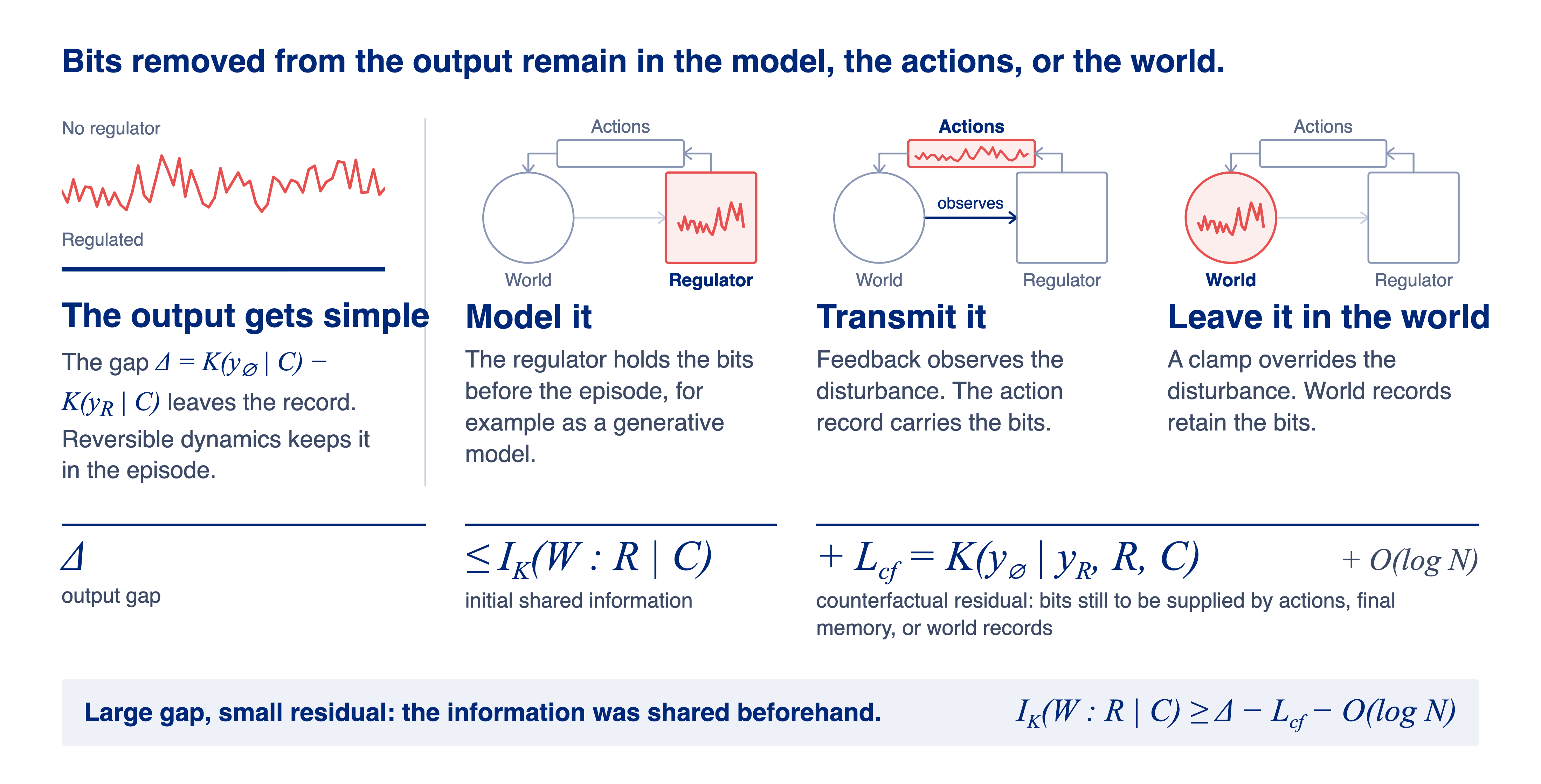
The idea that successful regulation requires an internal world model helps motivate both the generative models of active inference and the modeling engine of Kolmogorov Theory's algorithmic agent. Conant and Ashby's good regulator theorem and the internal model principle support this idea under specific assumptions. We ask when successful regulation implies that a regulator already contains information about the world. We compare finite output records of the same world with and without regulation, holding initial world conditions, disturbance inputs, and measurement rules fixed, and quantify the complexity reduction using prefix Kolmogorov complexity. Our starting point is precise information accounting, organized through an information-conserving logical construction. A computable reversible realization preserves the descriptions needed to recover the initial world and reconstruct its uncontrolled output. This realization may be auxiliary: physical determinism and reversibility are not general requirements of the resulting finite-record bounds. The Good Algorithmic Regulator Theorem (GART) bounds the reduction by the mutual algorithmic information initially shared by world and regulator plus a counterfactual residual, up to logarithmic coding overhead. The residual is the additional description needed to reconstruct the uncontrolled output given the regulated output and the regulator's initial description. A large reduction therefore requires substantial initial shared information when the residual is independently bounded well below the reduction. When actions, final regulator memory, and complementary world records suffice for reconstruction, they account for the residual: model it, transmit it, or leave it in the world. A generative-model example makes the output constant while preserving reconstruction information; feedback and clamps can also yield large reductions, with information carried by actions or retained in the world. Compact intervention knowledge can sustain regulation while supplying little additional compression of the uncontrolled record. The deterministic bound applies to individual finite records without a disturbance distribution or a prior over programs. The earlier Algorithmic Regulator Theorem (ART) bounded the posterior weight of a specified world–regulator explanation, but a fixed-clamp family with nonvanishing posterior mass defeats its unrestricted aggregate inference. Conditioning on a bounded residual guarantees, under any probability law on admissible world–regulator pairs, that initial shared information cannot fall below the reduction by more than the residual bound and coding allowance. For independent initial draws from fixed computable laws, an exponential bound limits the probability of a large reduction with a small residual.
Keywords:
algorithmic information theory
; Kolmogorov complexity
; regulation
; Good Algorithmic Regulator Theorem
; mutual algorithmic information
; counterfactual residual
; information conservation
1. Introduction
A regulator keeps a chosen aspect of a system within an acceptable range despite disturbances. A thermostat holds temperature near a target; a physiological circuit maintains a variable within a viable range. We ask what successful regulation, observed from outside, establishes about the information a regulator contained about the world before regulation began.
Even the same constant output can arise through different mechanisms. A regulator may already contain a generative model of the relevant world dynamics and use it to cancel predictable variation. Another may use a much shorter intervention rule to activate regulatory machinery already in the world, as when an agent switches on an air-conditioning system. A feedback regulator can also acquire disturbance information as it acts; a clamp can leave that information in the world. The generative model and the compact intervention rule both embody initial world information, but knowing how to intervene need not amount to describing the uncontrolled trajectory. The question is how much the regulator initially shares with the world, and how information acquired or retained elsewhere supports the same output reduction. Observing a simple output does not, by itself, distinguish these mechanisms.
The idea that regulation requires an internal world model helps motivate both Kolmogorov Theory and active inference. In Kolmogorov Theory, an algorithmic agent has a modeling engine (ME), an objective function (OF), and a planning engine (PE): it learns world regularities and uses them to select actions that support its persistence [1]. Active inference likewise connects perception and action through generative models and a free-energy objective [2,3]. Conant and Ashby’s good regulator theorem identifies a model relation for the simplest optimal regulator in its setting [4].
Ashby related regulation to reducing the variety of outcomes, measured by entropy, with constancy as the limiting case; his law of requisite variety bounds that reduction by the regulator’s own variety [5]. The Algorithmic Regulator Theorem (ART) brought this viewpoint to finite records [1]. Regulation as compression concerns the record that expresses the task. For stabilization, this can be the deviation from a setpoint; for tracking, the deviation from a prescribed trajectory; for homeostasis, the departure from a viable range. The target, output rule, and absolute measurement resolution are fixed before comparing regulation with its absence. Exact tracking produces zeros even when the reference trajectory is complex. Remaining within a prescribed range likewise makes its violation record zero. At a fixed measurement resolution, restricting deviations to a narrower range can shorten their range codes. Several task variables can be recorded together. This gives a common information criterion for maintaining desired conditions and following desired changes.
Write for the prefix Kolmogorov complexity of a finite record y: the bit length of its shortest self-delimiting program on a fixed universal machine. Such a program identifies its own end. A constant record has a short description once its length is given. Comparing uncontrolled and regulated records asks how much simpler the intervention makes the selected output, without assuming a disturbance distribution. The declared target gives this simplification its regulatory meaning: a constant wrong deviation is simple but unsuccessful, and an already simple null record leaves little possible complexity gain. A lossless compressor supplies an upper bound on K, including the fixed cost of its decoder, not its exact value.
Let W and R describe the world and regulator, including their programs and initial data. They exchange observations and actions over N steps. One world output channel supplies the regulated record . Its matched null, , is the record from that same channel when the tested regulatory contribution is disabled. The world program, initial world data, disturbance inputs, observation rule, and horizon remain fixed. For a thermostat, W can comprise the room and external disturbances, with sensing and control assigned to R.
The information account is guided by a reconstruction argument. In a computable reversible realization, the complete final state and elapsed time determine the initial world [6]; running its specified null episode recovers the uncontrolled output. Section 3 distinguishes this logical construction from the records supplied by a particular system. The output gap compares two alternative episodes; it is not a measure of information destroyed during one episode.
To express what this implies about the initial regulator, we introduce the counterfactual residual: the additional description needed to reconstruct the uncontrolled output given the regulated output and the regulator’s initial description. A small residual means that these already supply nearly everything needed for reconstruction. A large residual need not indicate poor regulation; it means that much of the uncontrolled record remains unspecified by those two descriptions.
The Good Algorithmic Regulator Theorem (GART) bounds the output complexity gap by the mutual algorithmic information initially shared by world and regulator plus this residual, up to logarithmic coding overhead. A large gap therefore requires substantial initial shared information when the residual is independently bounded well below that gap. Following ART, a regulator is good for the chosen output when it makes that output simpler than the matched null; the name echoes Conant and Ashby’s theorem. Sufficient episode records make the residual concrete. A retained generative model can reconstruct the uncontrolled record and guide compensating actions; because the model is part of the initial regulator, it bounds the residual independently of the gap. Online cancellation can instead record newly observed disturbances in actions, while a short clamp command can leave the disturbance information in the world. The examples show how these contributions support the same simple output.
ART bounded the posterior weight of a specified world–regulator explanation [1], but this does not control the total weight of a class of explanations. Appendix A.3 proves the failure of its unrestricted aggregate inference. GART supplies a residual-conditioned replacement under any probability law on admissible explanations (Corollary 4). A separate exponential bound concerns the chance of a large gap with a small residual under independent initial sampling (Appendix A.5). The first result concerns what the evidence implies; the second concerns how often such an episode arises from independent choices.
GART constrains initial shared information rather than prescribing a modeling architecture. The core finite-horizon results have Lean-checked counterparts under explicit algorithmic-information and decoder hypotheses (Appendix F).
Section 2 fixes the regulation setup and coding conventions. Section 3 derives reconstruction from complete-state conservation. Section 4 establishes GART, illustrates the different mechanisms for the same output gap, and develops the sustained and probabilistic forms. Section 5 discusses internal models, system boundaries, intervention knowledge and descriptive power, earlier regulator theorems, and measurement limits; Section 6 summarizes the findings and the question of model acquisition during ongoing regulation. Appendices Appendix A–Appendix D provide the probabilistic arguments, exact identity, rate limit, and intervention and measurement details. Appendices Appendix E and Appendix F collect the notation and formalization record.
2. The Regulation Setup
The formal comparison keeps the experimental description fixed. Let C denote the common coding frame: the system boundary, generic interaction and output conventions, target reference, measurement precision, null intervention, and shared encoding and simulation rules. These choices precede the particular episode. A target temperature may belong to C; the particular world program, initial conditions, and disturbance inputs belong to W. Problem-specific actuation semantics, which command reaches which device and what that device does in this world, also belong to W, not to C. Any corresponding model, key, or intervention rule initially held by the regulator belongs to R. The common frame specifies how to interpret the descriptions; it does not supply the problem-specific knowledge whose initial presence is being assessed.
The description R specifies the regulator’s program and initial data, including any preloaded memory. Information acquired later belongs to its evolving state. Thus W and R describe machines with their inputs, rather than only their work tapes.
Let be the whole modeled system, partitioned into the world and regulator. We also use W and R to name these subsystems; in complexity expressions they denote their finite initial descriptions. Write and for their complete encoded states at time t, with joint state
The model assigns shared communication tapes and retained output and action records to the world side. The regulator state contains its program, private data, working memory, and current execution state. These assignments specify what belongs in each state; they do not require each component to be experimentally observable.
Figure 1 shows this partition in the regulated and null episodes. In each panel, the lower tape records the world output being compared, while the upper tape records regulator actions.
Conditional complexity is the shortest program length for producing u when v is supplied without charge. Throughout, abbreviates , so the horizon is supplied in every comparison; we occasionally display N explicitly to emphasize a length-indexed family. Mutual algorithmic information measures the saving from a joint description rather than separate descriptions,
Here A and B are finite records, and describes their encoded pair. We call the initial shared information. It measures world-related information already present in R, which need not take the form of a symbolic model or a common extractable string. Reuse across episodes requires a separate test.
In the generating description, the programs and initial data in W and R specify a deterministic finite interaction, with the same finite disturbance inputs included in W in both episodes. For a computably specified stochastic model, the required realized random inputs must be included in the descriptions and their use across the two interventions fixed. Later observations acquired by the regulator belong to the episode records, not to its initial description R. Write for the scored world output after N steps and define
A positive gap means that the regulated record is simpler. The generating description supplies two distinct properties: null-output computability, a fixed rule producing from , and regulated-output computability, a fixed rule producing from . The world-information form of GART uses the first; ART’s specified-explanation posterior also uses the second. Four names recur. The good regulator theorem (GRT) is Conant and Ashby’s. A good algorithmic regulator (GAR) is one with , Definition 2 of the original article. ART is that article’s probabilistic bound on a specified explanation of a GAR’s output. GART, the present theorem, bounds a GAR’s initial shared information in terms of the gap and residual.
All description-length comparisons allow fixed interpreter costs. Concatenating prefix programs, and applying a fixed computable map inside a conditional complexity, cost constant overhead. Two-sided chain-rule identities with ordinary strings as side information introduce an additional logarithmic tolerance. We also use data processing for mutual algorithmic information at this tolerance [7], without needing a sharper bound. We write it as when the total encoded sizes in a statement are bounded polynomially in N. Otherwise it is , where bounds those sizes. The rate results require , meaning that this overhead divided by N tends to zero. Fixed additive constants cover small horizons; an allowance may include smaller constant costs, distinguished in the proofs where useful. Table A1 in Appendix E collects the symbols as a reading aid.
Connection to statistical measures. This finite-record criterion also connects to the usual statistical measures. For a computable stationary ergodic source on a finite alphabet, complexity per sample converges almost surely to the Shannon entropy rate [7]. For independent Gaussian errors measured at fixed resolution fine relative to their standard deviation, reducing variance reduces the asymptotic coding rate. For correlated Gaussian errors the corresponding rate depends on the spectrum, so variance alone does not determine it [8, Sections 9.1, 9.3, and 11.5]. These are statistical limits of the coding criterion; the finite-record comparison also applies to transients and individual episodes.
3. Conservation and Reconstruction
The guiding principle is logical information conservation: descriptions needed for reconstruction are retained as declared background or counted as additional information. The construction may be an auxiliary simulation; the results use their stated premises rather than general assumptions of physical determinism, reversibility, or storage. Interpreting the account as information retained in the original system requires the supplied descriptions to represent that system’s records. Table A3 collects the result-specific dependencies.
3.1. The Information-Conserving Construction
Assume, for this construction, a fixed computable execution law F with a computable inverse, and let T be a supplied signed time offset. Include F and the state-encoding conventions in C. The state is the complete state of the chosen realization. The execution law interprets the world and regulator programs carried by their states; it does not supply their problem-specific actuation semantics. Forward and backward computation give
and hence the global conservation law
Computable determinism supplies the forward computation; computable reversibility supplies recovery of the past [6]. Without an inverse, a fixed computable forward evolution gives only non-growth of complete-state complexity, with its inputs and time offset supplied. Equality of complexity values alone would not supply a reconstruction algorithm.
For the world–regulator partition, the definition of mutual information gives
Using Equation (5) with the same time offset supplied throughout, subtracting this identity at two times shows that changes in the two marginal complexities sum to the change in their shared information, up to fixed coding overhead. This is the complete-state conservation balance. A decrease in one marginal complexity must be accompanied by an increase in the other or a decrease in their shared information. The latter occurs, for example, when a retained model cancels a world record it already describes. The complete state still retains the information, although a selected output need not. To compare that output with its uncontrolled alternative, we recover the initial world and run the specified null episode.
Ordinary Turing-machine work tapes can be overwritten. Bennett’s construction realizes the same computation in an auxiliary deterministic, reversible machine, retaining the input and output after uncomputing its temporary history [9,10]. At the level of endpoint descriptions, let P be a program, u its supplied input, and its finite episode record under a fixed computable simulator. Then
since one direction computes the record and the other retains . Bennett’s construction supplies a stepwise reversible realization, rather than this endpoint equality alone. Levin’s information non-growth and Zurek’s account of description length and erasure provide related foundations [11,12]. Thermodynamic reset costs require an additional physical model, as discussed in Pattern, Persist! [13].
3.2. Logical Reconstruction and Episode Records
An auxiliary description can be used in a proof without existing as a physical record. Let be any finite description supplied in addition to . It suffices for the comparison when
For example, if the null output is computable from W, taking guarantees reconstruction whether or not the world retains its initial description. This does not make the counterfactual residual small: is additional information and its required description must be counted. Prefix-program concatenation gives
Thus an auxiliary description is not supplied for free in C or added to the initial R.
For the episode interpretation, the chosen output is only part of the regulated episode. Write for the regulator output (action) sequence and for its final private state, including memory. A complementary world record selects information in the final world state outside the chosen output, such as retained disturbance inputs or work-memory contents. A fixed computable projection specifies the selection,
The rule belongs to C and is fixed before the comparison. It selects information already present in the regulated episode. The tuple supplements the single chosen output; its components need not be separately measured or accessible to the regulator. The alternative name world exhaust refers to information omitted by that output, without implying heat or information crossing the world boundary.
The required reconstruction has a specific target: generate the uncontrolled output from the regulated output, the initial regulator description, and these additional records. Recovering the complete system is sufficient, but a smaller collection can suffice for this one output.
Definition 1
(Reconstruction condition). For the finite tuple , the reconstruction condition is
The conditional complexity counts the extra program bits needed after the listed records have been supplied. The records themselves can be large, and the computation can take arbitrarily long. The condition therefore expresses short-description recoverability, not inexpensive measurement or fast prediction.
3.3. Reconstruction from a Complete Reversible Realization
For complete records of the chosen realization, a computable left inverse of the finite evolution suffices to recover its admitted initial states. It need not invert each intermediate step or satisfy a right-inverse identity. A reversible evolution supplies such a rule. The common frame contains the fixed rules and encoding conventions, while the particular world description and initial state remain in the supplied records.
Proposition 1
(Reconstruction from a complete reversible episode). Suppose for a fixed computable evolution F. Let G be a fixed computable recovery rule satisfying for the admitted initial states s and horizons N. Let encode by the convention fixed in C, and let a fixed computable rule generate from W under the specified null protocol. Include F, G, and these conventions in C and supply N. If the supplied records recover the complete final state within the coding tolerance,
then the reconstruction condition in Definition 1 holds.
Proof.
With C and N supplied, the reconstruction is the sequence
The first step uses Equation (9) and costs additional description bits. The second applies to recover ; this is the only use of the left-inverse hypothesis. The third reads the initial world program and inputs by the encoding convention. The last simulates that world under the declared null intervention. These last three steps are fixed algorithms supplied by the conventions, so their descriptions and composition add only bits. The total reconstruction cost is therefore . □
Interpretation. Complete records determine both outputs through the initial world, but one output alone need not determine the other. Consider a reversible swap between a world register holding an incompressible disturbance d and an initially blank regulator register. The final world register is blank; the final regulator register holds d. Taking these world-register contents as the outputs gives a simple regulated record and a complex null record. The regulator’s final memory supplies the missing disturbance. Reconstruction says that this information can be recovered, not that its contribution is small.
Retained program and input records give another route: select them from and run the null episode afresh, even if work-tape updates were irreversible. For example, a world may retain a disturbance tape d and emit it only when a clamp is inactive. Selecting that tape gives . Other retained inputs can suffice without storing the null output itself. Reconstruction is weaker than full conservation: an unrelated register may be erased while the null output remains recoverable.
An external archive can supply an auxiliary description, with its information counted, but it is a world record only if the archive belongs to the declared system. Adding it to the system changes that boundary.
A physical application must justify the corresponding reconstruction. For a deterministic room-temperature model, the initial room conditions, governing equations, and the same recorded weather inputs permit a simulation with heating disabled. Constant regulated temperature alone does not supply those inputs. Missing weather records can make the proposed collection insufficient even when the heating system regulates successfully.
Figure 2(A) locates these records: the actions occupy the upper tape, the final private state remains in the regulator, and is the dashed region within the world. Panel B shows the matched-null episode; the reconstruction records come from panel A.
4. The Good Algorithmic Regulator Theorem
The balance compares what is known initially with what the episode records add. Given the regulated output and the initial regulator program and data, generating the uncontrolled output may require further information. The number of additional description bits needed is the counterfactual residual.
Definition 2
(Counterfactual residual). For any specified finite regulated and null records, the counterfactual residual is
It counts bits of description, not actions or compatible alternatives.
The relevant contribution of is its information about the uncontrolled output, conditional on the regulated output and initial regulator. The chain rule expresses this as a saving in description length,
The first complexity is the residual; the second is what remains after is supplied. Under reconstruction, the second is only coding overhead, so
An unrelated complex record contributes little, and information already available from R is not credited again.
For example, a short feedback program can cancel each disturbance bit after observing it. Its regulated output is all zeros, but its actions record the disturbance sequence. Those actions can therefore supply the information needed to reconstruct the uncontrolled output, even though the initial program did not contain that sequence. The theorem states the corresponding bound for any sufficient collection of records.
Theorem 1 (Good Algorithmic Regulator Theorem (GART)). Fix the coding frame C and horizon N, with the size convention of Section 2. Let be finite descriptions, define by Equation (3), and let be a finite record tuple satisfying (Definition 1). For the second inequality, assume additionally that a fixed computable rule produces from . Then
Proof.
We first bound the gap using the residual, then identify the residual’s contribution in the episode records.
First, separate what the initial regulator shares from what it leaves unspecified. One description of the pair first generates R, then generates with R supplied. Since the two programs are self-delimiting, concatenating them costs only a fixed wrapper,
The definition of mutual algorithmic information rearranges exactly to
Substitution therefore gives
Second, describe what is still unspecified through the regulated output. Given R, generate and then run a shortest residual program for given . The same concatenation argument, and the option of ignoring R when generating , give
Up to this point the proof uses only finite descriptions.
Finally, use the episode records and the world description. Under Definition 1, Equation (12) identifies the residual with the conditional information supplied by , up to . This proves the first inequality of Equation (13). The fixed null simulator computes from W, so algorithmic data processing gives
Substitution proves the second inequality. The record bound includes the reconstruction tolerance and the two-sided conditional chain rule used in Equation (12); data processing is used at the same logarithmic precision. The concatenation bounds use only constant overhead. □
Interpretation. A large output gap requires substantial information already shared by the world and regulator when the additional records contribute little to reconstructing the uncontrolled output. The same inference can be stated directly in terms of an upper bound on the residual, using Equation (16) even when the chosen records are insufficient.
Exact form. The inequality is the projection of a finite-string identity. For arbitrary finite ,
(Proposition A4, Appendix B). The two subtracted terms are the regulated output’s information about the regulator and the cost of producing the regulated output from the uncontrolled one and R. GART drops them; for a constant regulated output both are coding overhead and the first inequality in Equation (13) is tight. The same identity at the level of the world description, with in place of , is Equation (A6) in Appendix A.
Corollary 1
(Initial-information and residual bounds). For the finite-record comparison of Equation (3), assume that the null output is computable from by a fixed rule. If , then
For arbitrary finite , without the null-output computability assumption,
Proof.
For the first inequality, use null-output computability to replace in Equation (16) by , substitute , and rearrange. For the second, use the direct bound in the same residual inequality and rearrange. □
Interpretation. A gap of 1000 bits and a reconstruction program using at most 100 additional bits imply at least 900 bits of initial shared information, minus coding overhead. The program receives and R; every further input counts toward the 100-bit allowance. Because R includes its initial data, preloading the disturbance can satisfy this bound. The result establishes shared information, not by itself a reusable predictive model. Conversely, a short initial regulator facing a large gap leaves a large residual. Along a family where the residual bound and coding overhead are negligible compared with the gap, the initial-information lower bound approaches the gap.
At any horizon satisfying Theorem 1, its second inequality rearranges to
Comparing horizons requires removing the horizon from the side information on the left.
Corollary 2
(The bound across horizons). Fix the pair and a background that excludes N, with all side information explicit; the abbreviation of Section 2 is not used. Let be a nonempty set of positive horizons with a uniform null simulator and residual bounds . Write , and let cover the per-horizon coding allowance. Then, for a fixed independent of N,
Proof.
Corollary 1 gives at each admitted horizon. To remove the horizon from the left side, prefix-program concatenation gives
Each marginal complexity can only decrease, up to a fixed constant, when N is supplied. Substitution in the definition of therefore gives . Combining the two bounds at each horizon and taking the supremum proves Equation (21). □
Interpretation. Under uniform polynomial-size conventions, the combined coding costs are bounded by for a fixed c. The horizon penalty cannot be dropped when the initial shared information is measured without N. The strongest bound need not occur at the largest tested horizon. For a fixed finite world, simulation gives ; this is an upper bound, not a claim that output complexity reaches it. The gap, residual, and coding costs must be compared together. In the short online-cancellation and clamp examples, the residual accounts for the large gap, so increasing the horizon does not force growing initial shared information. This bound concerns one fixed pair; it does not pool the growing world family of the rate result in Appendix C.
Remark 1
(Incomplete reconstruction). For any finite tuple , the conditional chain rule gives
4.1. Lossless Regulation Through a Generative Model
A model can preserve a long output record through a short generating rule and its parameters. Suppose the initial regulator contains , where g is a computable generator and is its finite parameter record. The model generates the uncontrolled disturbance record d at the declared resolution and horizon,
For example, a specified periodic thermal forcing can be represented by a waveform rule, amplitude, period, and phase. The parameter precision and any initial conditions needed for exact reconstruction are part of M, hence of R; the common frame supplies only the fixed coding and evaluation rules. When this description is shorter than listing the samples, it compresses the entire record losslessly.
Assume an additive output channel with sufficient actuation to compensate for this predicted disturbance. Its finite encoded samples permit exact addition and subtraction. At step t, the regulator generates from M and sends the action , giving
The null action is zero and leaves d as the output. The regulator retains M. This logical operation is reversible: for any sample record v,
has the inverse that adds . Consequently,
The scored output has become constant while the retained model and parameters still recover every sample of the uncontrolled record. No information erasure or growing store of new episode data is required.
This construction also supplies the residual bound independently of the observed gap. A fixed program reads M from the initial R and runs its generator, so
The additional records contribute only coding overhead. The gap is and is bounded by the model’s description length up to fixed overhead; a long generated record need not have one independent algorithmic bit per sample. The model can therefore support arbitrarily long predictable episodes without growing with their raw duration. Appendix F records the checked compensation and reconstruction steps. These ideal assumptions concern the available model and actuator; they do not assert that an arbitrary feedback device predicts every disturbance.
A thermostat can embody a less detailed model in its calibrated response: the selected action brings the next temperature closer to the target. At a fixed resolution, deviations from to occupy 101 levels, while deviations from to occupy 11. A direct range code needs seven versus four bits per sample, with the range specified once. This code is lossless for the measured record. If all readings occupy the target bin, the record is constant. This gives a finite-resolution coding interpretation of successful regulation; the model-and-parameters construction above also shows how the information remains recoverable.
4.2. Different Mechanisms for the Same Output Gap
Let d be an incompressible disturbance sequence of N bits. In every scenario in Table 1, the uncontrolled output is d and the regulated output is the all-zero sequence,
Table 1 separates initial shared information (second column) from the additional contribution of episode records (third column); its last column identifies a sufficient source of d. Since N is given, the zeros supply almost no information about d. The contribution of is therefore determined by how much it reveals about d beyond the initial regulator description.
For cancellation, each output bit is the exclusive OR (XOR) of the disturbance and action bits: it is zero when they agree. A preloaded regulator stores d initially and supplies each matching action. An online regulator instead observes each disturbance bit before acting. Both produce zeros, but the first uses initial data while the second acquires the disturbance information during the episode and records it in its actions.
A blind clamp sends a fixed command that holds the output at zero while d remains in the world. A clamp with private retention also observes and stores d through a declared observation channel, separate from the output being evaluated. Its final memory then specifies d. Both private retention and preloading require storage growing with N. The preloaded row is a valid finite-episode benchmark, but one bounded store cannot supply arbitrarily long fresh incompressible disturbances. Section 4.3 states the consequence for sustained regulation.
The last row uses a world containing d and a key of length n, with incompressible given their lengths and C. The world emits d unless it receives before the first output. A regulator holding the key makes this one intervention, leaving d in the world record. The right-hand side of GART is about bits for a gap of about N; the bound need not be tight. Section 5.1 explains the compact intervention knowledge this example can represent.
Initial data and episode records can each supply part of the required information. Few actions do not by themselves make the residual small: one precisely specified action can contain many bits, and further information can remain in private memory or the world.
4.3. Episode Records and Sustained Regulation
The conditional chain rule separates what the supplied records contribute,
Each term credits information about the uncontrolled output that the preceding records did not supply. The order changes the allocation, but not the total: duplicated information is counted only once, and unrelated complexity earns no credit. This is a description account, not a unique causal assignment of bits to actions, memory, and world.
A regulator is cyclic when its private state ends the episode in a fixed reference state, as a thermostat or a finite-state feedback controller does after each control step: whatever it observed has been acted on and cleared, so its final memory costs only coding overhead to describe once the initial description and the execution conventions are given, . The case matters because it removes the private-memory channel from the split in Equation (29), leaving exactly the three sinks named in the title: any disturbance information such a regulator acquires must appear in its actions or remain in the world. It is the regime of the online-cancellation and clamp rows of Table 1.
Corollary 3
(Regulation balance for a cyclic regulator). Let satisfy , and assume a fixed computable rule produces from . If , then
Proof.
Insert the split in Equation (29) into the second inequality of Theorem 1. Conditional mutual information is at most the conditional complexity of either record, so the memory term obeys
by the hypothesis. Absorb this term into the coding allowance. The action and complementary-world terms remain, giving Equation (30). □
Interpretation. An online cancellation regulator can observe a disturbance bit, issue the matching action, and reset its working memory. Its final memory is simple, but its action sequence still specifies the disturbance.
Sustained regulation. For sustained operation, the initial information must also be compared with the growing episode length. The fixed model in Section 4.1 can generate a long record from bounded data. Fresh incompressible disturbances impose a different requirement. A fixed finite regulator has bounded initial information. If the output gap grows proportionally to the horizon while retained private information grows more slowly, actions and complementary world records must supply the increasing amount. This is GART divided by the number of steps; Appendix C gives the rate definitions and limiting argument.
For incompressible length-N disturbances, online cancellation produces a gap approaching one bit per step and an action contribution of one bit per step, with negligible final memory. A blind clamp with simple actions instead leaves one bit per step in the complementary world contribution. Memory retaining disturbance bits grows with the episode but contributes zero in the rate limit; its finite contribution can be smaller if the actions already specify those bits.
A positive asymptotic gap rate requires a family of worlds with growing disturbance data. For one fixed finite deterministic W, simulation gives , where is its null output at horizon N. Its gap per step therefore has no positive limit superior. The growing family makes precise the fresh-input setting in which a bounded preloaded store cannot sustain the cancellation row of Table 1.
4.4. The Probabilistic Reading
ART asked how likely a regulator is to share little information with its world, given the regulated output. Its proposed exponential tail in the shortfall below the gap does not follow from the specified-code bound: a fixed clamp regulating a family of complex worlds retains nonvanishing posterior mass (Appendix A.3). GART identifies a sufficient additional premise. Write for initially shared information, for the gap, and for the residual; all three vary with the explanation .
Corollary 4
(Probabilistic ART, conditioned on the residual). Let Π be any probability law on a countable class of admissible world–regulator explanations, and let E denote the supplied evidence. Let the residual budget η and uniform coding allowance h be nonnegative integers. Suppose and the pointwise residual bound holds throughout this event. Then, for every integer deficit ,
The probability on the left is zero when .
Every explanation retained by the conditioning satisfies , so the event is empty once ; for smaller k the bound is one. Appendix A.4 gives the proof, ART’s posterior normalization, and the variants with uncertain or explanation-dependent allowances.
Interpretation. The deficit k measures how far shared information falls below the gap. The residual budget bounds the description still needed for the uncontrolled record given the regulated output and initial regulator; h is the coding allowance. A gap of 1000 bits with a residual of at most 50 bits therefore requires at least bits of initially shared information, with probability one under the conditioned law. The exponential display recovers ART’s proposed form, with the residual and coding allowances setting the threshold; the deterministic exclusion beyond it is stronger.
The inference depends on establishing a small residual. A fixed reconstruction program, together with a short description of the episode records it uses, supplies an upper bound on L. A residual bound known with confidence transfers that confidence to the information bound; Appendix A.4 also treats exponential residual tails. The additional premise concerns recoverable information in the episode, and cannot be supplied by universal weighting alone.
The bound is one-sided: the shortfall can equal the residual, as the partial-preload example shows (Appendix A.4). The allowance h must be uniform over the conditioning class; its possible horizon dependence is discussed there.
A separate question concerns how often independently chosen worlds and regulators produce a large gap with a small residual. For fixed computable sampling laws specified in C, the probability of a gap of at least with residual at most is at most (Proposition A3, Appendix A.5). Guessing a uniformly distributed N-bit cancellation sequence succeeds with probability , while a clamp succeeds routinely because its residual is large. The corollary concerns what the evidence implies; this sampling bound concerns how rarely the required initial information arises by chance.
Remark (the posterior on the small-residual class). The exact specified-code posterior in Equation (A9) charges three description costs: the regulator given the output, the residual, and the world information still unspecified by the two outputs and regulator. Restricting bounds the residual factor between and one, within coding tolerance. The remaining world-description cost still matters: a small residual alone does not reduce the posterior to a weighting by regulator complexity only. The clamp family is excluded by the conditioning event, not outweighed inside it.
5. Discussion
5.1. Models and System Boundaries
GART gives a quantitative condition under which regulation requires initial information about the world. A large output gap and a small counterfactual residual force substantial mutual algorithmic information: supplying the regulator then shortens the world’s description by at least the gap minus the residual and coding overhead. This is model content in the compressive sense developed in Models, networks and algorithmic complexity and the parametrized account of algorithmic emergence [14,15]. In the generative example, a rule and parameters preserve the uncontrolled record losslessly and repeatedly guide compensating actions. The same representation serves compression and regulation, connecting the balance to the reusable parametrizations studied in Pattern, Persist! [13]. Its Algorithmic Persistence Balance applies the same chain-rule account to a pattern’s own persistence. The example assumes the model is available; acquiring it remains a further problem. It also gives the agent architecture a concrete reading: the retained generator supplies the modeling engine, the zero-deviation target the objective function, and the compensating action rule the planning engine’s policy.
An intervention model can instead specify how to recruit machinery already in the world, as when a remote command activates an air-conditioning system. Section 5.2 separates this compact world knowledge from the ability to describe the uncontrolled record.
The system boundary determines where this information is counted. When a short command delegates regulation to a thermostat or homeostatic circuit within the world, that circuit’s disturbance-dependent records contribute to the world record. Including the circuit in the regulator changes their place in the balance. Under our convention, C contains generic encoding and execution rules, not the problem-specific fact that a particular command activates this circuit. That fact is encoded by the world’s mechanism and, to the extent initially known, by the regulator’s model or intervention rule. A world-specific key held by the regulator likewise belongs to its initial data. A short rule can still carry little shared information compared with the disturbance record; it is counted rather than conditioned away. Appendix D.1 gives the key-information bound, and Appendix D.2 distinguishes the two directions of interaction in a thermostat loop.
The same balance applies when the regulator controls another part of its own agent. With that part’s null output computable from its declared initial description, a large gap requires substantial initial shared information whenever the residual is independently bounded well below the gap.
5.2. Intervention Knowledge and Descriptive Power
Compact intervention knowledge is still world information. A calibrated thermostat, remote control, or clamp embodies a task-relevant relation between an action and its effect. The rule can remain effective as disturbances change while specifying little of their detailed history. The distinction is between knowledge of how to intervene and a description of what would happen without intervention.
To quantify an embodied correspondence, suppose fixed computable extraction rules recover the same finite descriptor m from W and the initial R, . It may specify a world-specific key or a declared calibration rule; its recoverability from both descriptions is the premise. The argument of Appendix D.1 gives : apply data processing to both extraction maps and use . With null-output computability, Corollary 1 supplies the complementary bound. Under the size conventions of Section 2, together they give
The two lower bounds are not added, since they can concern overlapping information. The descriptor bound can remain informative when the residual accounts for the gap. For a simple rule its contribution may lie within the coding allowance; a large residual does not establish the absence of an intervention model.
Supplying the initial regulator as side information can shorten the description of the uncontrolled output. This additional saving is , and the information account bounds it on both sides,
For the first inequality, subtract the bound of Equation (15) from . For the second, the chain rule identifies the description saving with within coding tolerance; null-output computability gives the upper bound by data processing. The middle quantity measures the additional saving obtained by supplying the initial regulator, not compression already available from the uncontrolled record’s own regularities. A regulator can therefore make the selected output simple while supplying little extra information with which to describe its uncontrolled alternative. A clamp suppresses the disturbance’s appearance in the selected output; the retained generative model can additionally reconstruct the disturbance. These are different achievements, even when both produce the same all-zero record.
The content of the shared information also matters. Since is computable from W, adjoining it to W costs only fixed overhead. Expanding mutual information in the order gives
The first term concerns the uncontrolled record; the second concerns shared world information beyond that record. In the short-key example, the key is algorithmically independent of the disturbance record: it contributes to the second term while providing negligible savings on the disturbance description. That term can contain other world information as well; it is not exclusively intervention knowledge.
More generally, the same upper-bound argument applies to any world record produced by a fixed computable rule, within the same size convention,
Small initial shared information therefore limits the additional world information the regulator can supply, not the number of tasks it can perform: different tasks may reuse one compact regularity, and ongoing observations may supply further information. The gap–residual balance identifies when regulatory success itself certifies substantial initial description savings.
5.3. Relation to Regulator Theorems
Table 2 distinguishes what earlier results call regulation, which conditions support their conclusions, and what world structure those conclusions require. In Conant–Ashby, the proof selects a deterministic optimal policy; the mapping can be constant when one action suffices. Baez’s critique and proposed entropy formulation expose the need to specify what such a model relation preserves [16]: being a function of the system state alone sets no lower bound on the world information retained. Francis–Wonham and Sontag impose stronger dynamical conditions and obtain generators of the relevant external signals. Sontag explicitly introduces signal detection to exclude a system that outputs zero for every input [17].
The internal-model results thus concern models of a relevant part of the world, such as the dynamics producing constant or periodic disturbances. Such a generator may have a short description, while the amplitude or phase of a particular input is acquired during regulation. Their structural correspondences require finite coding conventions and a specified world description before they can be compared quantitatively with shared information.
Touchette and Lloyd already give a necessity bound: feedback’s entropy reduction beyond the maximum available without observations requires at least that much state–control mutual information [19,20]. Their open-loop allowance admits clamps. GART similarly separates initial shared information from other contributions to simplification, but measures these through reconstruction of a matched-null record in one episode; its residual is not the Shannon maximization over channels and input distributions.
The coding-theorem identity in ART’s Theorem 3 also remains valid: the base-two logarithm of the ratio of universal a priori weights for regulated and null outputs equals the complexity gap up to fixed overhead [1]. This gives the gap an equivalent coding score; it does not establish that the regulator optimizes that score over available actions. Likewise, a deterministic regulator defines a history-to-action policy, without thereby establishing a planning mechanism. GART supplies the quantitative world-information requirement; identifying the full ME/OF/PE architecture requires evidence about how that information is used.
5.4. Measurement and Limits
The selected output must also represent the variable of interest: a constant thermometer display need not mean that room temperature has stabilized. Short reconstructions between the sensor record and the selected variable’s record provide a sufficient condition for transferring a complexity gap between them.
Let be a fixed computable rule in the common frame C selecting the variable’s recorded trajectory, and write for the null complexity minus the regulated complexity. Suppose the trajectory record and sensor record determine one another using at most additional program bits in each episode. Then
Appendix D.3 gives the precise conditions and derivation. A direct readout or fixed reversible encoding satisfies them with constant overhead. A display concealing an incompressible trajectory needs many additional bits for reconstruction, so its simplicity alone gives no corresponding guarantee about the trajectory. These conditions concern information in the records; physical calibration and attainment of the target require separate justification. A faithful readout can still have a large residual, as the blind clamp shows.
The declared resolution, target, and null intervention complete the comparison. When the supplied records omit reconstruction information, Remark 1 retains its description cost. Conversely, physical irreversibility does not invalidate a finite-string conclusion whose stated premises are satisfied. Reconstruction premises and measurement-transfer premises must therefore be justified separately.
Explicit programs upper-bound complexity, but the difference of two program lengths need not bound the true gap. Empirical applications therefore need a justified coding model or additional mathematical bounds. A thermodynamic interpretation requires further physical assumptions: resetting a record has a cost determined by its implementation and reset protocol [10,12,21]. The output gap itself is neither a count of erased bits nor a heat cost.
6. Conclusions
GART bounds the reduction in output complexity by information initially shared between world and regulator plus the counterfactual residual. The information-conserving logical construction guides the derivation, while each finite-record result rests on its stated premises rather than general assumptions of physical determinism or reversibility. Sufficient episode records identify how the residual is supplied by actions, final memory, and the world.
In the generative example, a compact rule and parameters reconstruct the uncontrolled record and guide compensating actions. Feedback and clamps illustrate alternative contributions from actions and world records. When the residual is independently bounded well below a large gap, substantial world information must already be present in the initial regulator. This answers the world-information question associated with Conant and Ashby’s theorem quantitatively: GART bounds how much information must be shared, without prescribing its representation or establishing its reuse.
Conditioning on a bounded residual supplies ART’s aggregate inference with the additional premise it needs (Corollary 4). Under any probability law on an admissible class with a bounded residual, initial shared information cannot fall below the gap by more than the residual bound and coding allowance; the unrestricted inference fails for the clamp family, whose disturbance information remains in the world. A separate exponential bound quantifies the chance of a large gap with a small residual under independent initial sampling (Proposition A3).
For algorithmic agency, a remaining question is how information acquired during ongoing regulation becomes a retained model that guides subsequent action, accounting for the costs of finding and retaining it.
The present analysis distinguishes regulatory effectiveness from the amount and content of initial world information. A compact intervention rule can embody knowledge of how to act while specifying little of the uncontrolled history. When the episode records suffice for reconstruction, actions, final memory, and world records account for the counterfactual residual. Bounding their contribution establishes how much initial shared information the output reduction requires. Thus successful regulation can rest on compact intervention knowledge, whereas a large reduction with a small residual certifies substantial information about the uncontrolled record and corresponding description savings (Section 5.2). Knowing how to intervene and being able to describe what would happen without intervention are related, but distinct achievements.
Funding
This research received no external funding.
Data Availability Statement
No new data were created or analyzed in this study. The Lean 4 formalization supporting the machine-checked results is openly available in the KTAIT repository, https://github.com/giulioruffini/KTAIT, at commit 6448b94 [22]. Appendix F records the correspondence between the results and the checked declarations and the scope of the formalization; the accompanying verification record reports the full build and the axiom audit, including the probabilistic extensions, of September 20, 2026.
Conflicts of Interest
The author declares no conflicts of interest.
Declaration of generative AI use
During the preparation of this manuscript the author used ChatGPT and Claude for manuscript criticism, mathematical consistency checking, restructuring, and language editing, and for assistance with the Lean 4 formalization. The author reviewed and edited all output and takes full responsibility for the content.
Appendix A. Probabilistic Regulator Bounds and the Clamp Family
This appendix restates ART’s specified-code bound [1], sharpens it using the residual, and separates individual code weights from aggregate posterior mass. Proposition A1 corresponds to the original Lemma 1 and Theorems 1–2, retaining the regulator-complexity factor in the sharper bound. We make the canonical code explicit, carry the frame and horizon, and treat null-output computability as a candidate hypothesis rather than extra evidence. The conditional-complexity form in the second line of Equation (A2) is an additional reformulation.
The original’s unnumbered aggregate claim after Theorem 2 was : M denotes its mutual algorithmic information, the class with null complexity b, and a constant. Appendix A.3 gives the counterexample. The new results are the two-sided residual refinement (Proposition A2), the residual-conditioned replacement (Appendix A.4), and the independent-sampling bound (Appendix A.5).
Appendix A.1. The Specified-Code ART Bound
The universal prefix-program prior gives a program p weight , where is its length in bits. For each candidate pair , choose one canonical code: a fixed simulation wrapper around a shortest description of the pair. Throughout this appendix x denotes the observed regulated output, , as in the original article and in Figure 1. Write for that code’s posterior weight after observing x: its prior weight divided by the total weight of all programs producing x. Distinct pairs have distinct codes; the evidence includes every program producing x, rather than only these selected codes.
Proposition A1
(Algorithmic Regulator Theorem: specified-code form). Let a fixed simulator produce from , and use the specified canonical-code posterior above for . Then
If its null output is computable from W under the fixed conventions, then
The positive constant depends on the fixed machine and simulation conventions, not on the candidate or horizon.
Proof.
Fix the frame and horizon. Throughout this proof, C includes the supplied N, as in Section 2. Let be the canonical prefix code for an explanation ; its length is . Denote by the universal evidence, the sum of the prior weights of all programs producing x. The coding theorem gives
This proves Equation (A1). A shortest description of W followed by the fixed null simulator describes , so , where . Substituting the defining identity yields
Exponentiation proves the first inequality in Equation (A2). For the second, expand the joint description in the order W, then R,
Substitute this identity into the exponent. The logarithmic allowance comes from the two-sided chain rule with the string W supplied. The null-complexity condition enters through the candidate’s simulation bound, not through the evidence denominator. □
Interpretation. Equation (A1) is the coding-theorem identity for a specified code. It compares codes for the same observed output, which share the evidence denominator: codes of 100 and 110 bits, for example, receive weights in the ratio , the shorter code receiving the larger weight. At fixed marginal description lengths for W and R, greater shared information shortens their joint description. Equation (A2) expresses the bound using the output gap: a complex null output requires a sufficiently descriptive world, and dependence can reduce the cost of describing that world together with its regulator. The statement concerns one specified code for each candidate pair.
Equation (A2) bounds the posterior weight from above; the residual supplies the matching lower bound.
Proposition A2
(Algorithmic Regulator Theorem with the residual). Under the conventions of Proposition A1, with computable from W and computable from , write , , and . Then, up to ,
The ceiling is ART’s: the weight of an explanation falls with its regulator’s length and its gap, less its shared information. The floor is the residual’s: the weight falls with the regulator’s length, the residual, and the world information beyond the null output. The floor meets the sharpened ceiling when shared information is at GART’s minimum . It meets the unsharpened displayed ceiling only when the hidden-world term is also coding overhead.
Proof.
Start with the specified-code identity, . To express it through initial shared information, use . Adjoining to W costs only a fixed null simulation, while projection recovers W. Expanding that joint description in the order , then W, therefore gives
Since , substitution gives
which implies the upper bound by dropping the nonnegative hidden-world complexity.
For the residual form, both outputs are computable from under the fixed rules. Adjoining them costs , and projection recovers , so . Expand this description in the displayed order, using ,
Substitute this expansion into the specified-code identity and compare with Equation (A7). Rearranging gives
Exact form. As with GART, the inequality is the projection of an identity. Equations (A7) and (A8) give the weight exactly, in two readings,
The first reading is ART’s exponent with the world information beyond the null output subtracted; the second has neither the gap nor the shared information and charges the regulator, the residual, and the hidden-world term. Equation (A5) drops the hidden-world term on the right and the excess on the left, as GART drops the two subtracted terms of Equation (A26). The second reading also gives : the posterior charges the residual bit for bit.
Interpretation. For the preloaded or generative examples with no substantial hidden-world term, and , where ≈ means equality up to : floor and ceiling meet at , and the explanation is charged its regulator and nothing else. Additional world data not specified by the null output retain their description cost. For the clamp family, and , with only fixed hidden-world overhead: floor and ceiling meet at , and each member weighs about . Between these, measures shared information that GART does not force, such as what the regulated output reveals about the regulator. Equation (A6) is GART with its slack named: because .
The hidden-world costs remain part of each explanation’s weight. Class probabilities require summing these weights, as the next two subsections show.
Appendix A.2. Conditioning and Aggregation
Let be the event consisting of candidate explanations whose null output has complexity b. If this information is supplied as additional evidence, Bayes’ rule gives, for a member e,
For a candidate belonging to , Equation (A10) follows from conditioning its posterior on that event. The reciprocal event probability cannot be absorbed into a uniform constant without a lower bound. Membership of one specified candidate does not make the event certain in a posterior over unknown explanations. For example, if 1000 explanations are equally probable after observing x and only 10 satisfy a newly learned event, each survivor’s probability rises from to .
For a threshold ℓ, the posterior mass of a class with limited dependence is
where candidates inconsistent with the evidence have zero mass. Bounds on individual summands do not imply an exponential tail for the sum without controlling multiplicity or aggregate weights. The construction below shows the failure of the concentration claim stated after Theorem 2 of the original ART article, the unnumbered tail bound quoted at the start of this appendix [1]. The finite arithmetic witnesses perpairdoesnotlift and multiplicitycancelspenalty check the generic summation issue; they do not separately formalize this concrete prefix-code construction.
Appendix A.3. An Explicit Lower Bound for a Clamp Family
A collection of individually unlikely explanations can have substantial total probability; the clamp family is an instance, built from many distinct codes with a lower bound on each one’s weight. Condition on N and a fixed frame C admitting length-N output records. Fix one memoryless regulator that always sends the clamp command. For each length-N string z, let emit z under the null and under the clamp, retaining z as world-side data. This is a variant of the latch construction in the original ART’s Appendix A.7 [1]. The original’s separate rarity estimate assumes a balanced coupling and a nearly uniform regulator interface; those hypotheses do not hold for this family. The clamp also exemplifies the many-to-one state transitions that permit entropy reduction without observations in Touchette and Lloyd’s account [20].
For a fixed integer , fewer than strings have a prefix program of length below given . Hence the set
has at least members. A fixed program can read N literal data bits, so uniformly. It follows that the null complexities in this family occupy a band of at most integer values. For some in that band, a subset of at least members has the same null complexity , where is independent of N.
A fixed constructor turns the N literal bits of z into the description of , and a fixed wrapper produces the regulated output record. Thus the specified canonical codes satisfy , uniformly. They are distinct prefix-program events, each of prior weight at least . Their total prior weight is therefore at least . Every one produces , and the universal evidence is at most one. Consequently,
All members have because has fixed complexity, but their common gap is . The subset lies within , so additionally conditioning on that event divides its mass by a probability at most one and cannot lower it. Therefore the low-dependence class has nonvanishing posterior mass despite an arbitrarily large gap. An exponential tail of the published form is false under this coding convention.
The family varies the world data, with one fixed clamp regulator; the multiplicity comes from the worlds, not from padded descriptions of one regulator. The result is compatible with the bound on each code and rules out the proposed concentration claim. In the deterministic balance, the disturbance information remains in an admissible world record from the regulated episode.
Appendix A.4. Conditional ART: Proof and Probability Conventions
Corollary 4 follows from the initial-information bound on each explanation. For and the fixed frame C, including the horizon N, the quantities introduced in Section 4.4 are
These quantities vary with the explanation. Let be an integer coding allowance for the GART inequality
The same allowance must hold throughout the class to which the statement applies. Under Section 2’s polynomial-size convention, .
Proof Corollary 4
Every explanation retained by the conditioning satisfies . Thus
If , the event is empty as well. If , the right side of Equation (31) is one and bounds any probability. All probabilities use the same positive conditioning denominator. □
Interpretation. If E also establishes a gap , then with conditional probability one. The factor is uniform across horizons only if is uniformly bounded; permits polynomial dependence on N. The deficit k measures how far information falls below the gap; the threshold measures the gap’s size.
The unadjusted event can still occur. For example, a regulator can start with most of a disturbance record, cancel that part, and clamp the remaining short part. The gap includes both parts, while the residual accounts for the part absent from the initial regulator. Increasing the known part increases the gap without removing that deficit. A small residual bounds this shortfall; it does not force I to equal or exceed the gap. Shared information about other world features can also make I exceed the gap.
For ART, take E to specify the observed output x, the null complexity b, and any declared class restriction. The gap is then . If is the selected canonical code for explanation e, its conditional probability is
This is the universal program posterior restricted to the indicated explanation event. The residual restriction enters the denominator as well as the numerator. No independence of world and regulator is required.
Uncertain residual bounds. If the residual budget is established with limited confidence, GART transfers that confidence to the information bound. When and Equation (A15) hold on E,
Thus the 1000-bit gap and 50-bit residual bound of Section 4.4, known with at least posterior confidence, give at least bits with the same confidence. A short reconstruction program and a short description of its additional episode records can establish the residual budget independently of this inference.
For classes requiring an explanation-dependent allowance , retain it inside the event. Whenever GART holds on E,
With , a separately established residual tail , for integers and constants , gives, for ,
This last bound uses probabilistic control of the residual in place of conditioning on a strict budget. Neither GART nor universal weighting alone supplies the assumed residual tail.
Appendix A.5. Chance Regulation Under Independent Initial Sampling
Before any successful episode is selected, independently chosen worlds and regulators are unlikely to produce a large gap with a small residual. GART reduces this question to the probability that independent draws share substantial algorithmic information. The following result uses prefix coding and the information–independence relation studied by Levin [23].
Proposition A3
(Chance regulation under independent initial sampling). Draw W and R independently from fixed computable probability laws and , with their algorithms supplied in C. Write . Suppose every pair in the sampling support has a declared output comparison and satisfies the pointwise residual bound wherever . There is a constant , depending only on the fixed coding and sampling conventions, such that, for every integer γ,
If , then
Here are nonnegative integers. The same constant applies across horizons when fixed algorithms compute the sampling laws from the supplied frame and horizon.
Proof.
Prefix coding for the two computable laws supplies constants such that
The constants cover the fixed sampling algorithms and coding conventions [7]. Distinct pairs have distinct shortest prefix programs, whose weights sum to at most one by Kraft’s inequality. The definition of I therefore gives
All terms are nonnegative, including for countably infinite supports. Set , a harmless enlargement of the moment bound that gives the normalization used in the statement. Markov’s inequality, applied to the nonnegative variable , gives
Interpretation. Each bit of gap beyond the residual and coding allowance halves the upper bound in Equation (A21), once it is below one. Conditioning on a small residual can select rare pairs, so Equation (A22) retains the selection probability . If the residual budget holds throughout the sampling support, . Neither statement is a posterior bound on after successful regulation is observed.
For example, draw two independent uniform length-N strings v and u. Let the null output be v, and let a regulator initially holding u produce . The residual is : the output and u recover v. Perfect cancellation occurs exactly when , with probability . For incompressible v, the successful pair has a gap and shared information of bits. Selecting these successes makes the initial descriptions correlated. A fixed clamp instead succeeds routinely with a large residual, while a regulator holding a learned or jointly designed model need not satisfy the independent-sampling hypothesis.
The variable-allowance form, useful when no uniform h is available, is
It follows from the same moment bound and pointwise GART.
Appendix B. The Exact Counterfactual Identity
The main proof bounds the output gap by dropping terms associated with the regulated output. The full finite-string identity retains these terms and shows when the bound can be attained. Replacing the outputs by the selected-variable records gives the same identity for that comparison.
Proposition A4
(Exact counterfactual balance). Let be arbitrary finite strings under the fixed coding frame and horizon. Define the gap and residual as in Equation (3) and Definition 2. Then
Proof.
First expand the joint description in the order R, then ,
Rearranging the definition of mutual information gives
and the same identity holds for . This equality uses the two-sided chain rule with ordinary strings supplied. It is consistent with Equation (14): that one-sided inequality requires only prefix-program concatenation and has constant overhead.
Next expand the pair in both orders, with supplied throughout,
Equating these expansions and rearranging gives
Interpretation. The subtracted terms quantify the regulated output’s information about R and the description needed to produce that output from the uncontrolled output and R. They need not vanish for arbitrary records. For the constant regulated output in Table 1, both are only coding overhead, and the identity reduces to the initial-information and residual account. The short-key row need not attain the world-information bound because can exceed .
The same identity written for the world description is Equation (A6), , where the excess collects the same two subtracted terms together with the world information beyond the null output, . The readout bound is tight, within coding overhead, when both and are coding overhead. Tightness of the world-information bound additionally requires to be coding overhead. A simple regulated record makes the first two terms small, but does not constrain this additional world information.
Under reconstruction, the finite deficit form is a rearrangement of GART,
It states how much the additional records must supply when initial shared information is small; the relevant quantity is their information about the uncontrolled output, not their total complexity.
Appendix C. The Rate Limit for Sustained Regulation
A fixed regulator cannot initially encode an unlimited amount of fresh disturbance information. Over longer episodes, consider a family containing the disturbance data for horizon N, with one fixed finite regulator R. Assume the reconstruction condition at each horizon under uniform coding conventions. Write and for the regulated and uncontrolled outputs of at horizon N; actions, final memory, and the complementary world record also refer to that horizon. A rate is the corresponding information divided by the number of steps. Let be the gap per step. Write and for the upper limiting rates of action information and complementary world information,
Corollary A1
(Rate form). For each N, let and be finite records satisfying the reconstruction condition under uniform coding conventions. If R has fixed finite description, (in particular, if the private memory is uniformly bounded), and the per-horizon additive coding slack is , then
Proof.
Start with the first (readout) inequality of Equation (13) and substitute the three-term split in Equation (29). The initial-information term is at most . Likewise, conditional mutual information is at most the conditional complexity of either record, so the memory term is at most . Let bound the combined coding allowance, as assumed. The finite-horizon bound we divide by N is therefore
The first term is bounded for fixed finite R; the second is by the memory hypothesis; and tends to zero. Divide by N and take the upper limit. The upper limit of the sum of the two information rates is at most the sum of their upper limits, defined in Equation (A31). This proves Equation (A32). The cyclic corollary is not needed: the present memory contribution may grow faster than , provided it remains sublinear. □
Interpretation. The initial description and sublinear final memory vanish from the rate bound after division by N. Online cancellation and the blind clamp in Section 4.3 attain the action and complementary-world alternatives, respectively. A bounded-memory regulator is a special case; unbounded memory can also have a vanishing rate contribution.
Appendix D. Intervention and Measurement Details
Appendix D.1. Initial Information in a World-Specific Key
The world’s program specifies where a command is sent and what it does; C supplies only the generic interaction and interpretation conventions. In the clamp example, this program and the matching command can both have fixed short descriptions. Their initial shared information can therefore remain small even when the disturbance record is complex. For the world-specific key in Table 1, suppose fixed programs recover the key , of n bits, from both W and the initial R. Applying data processing to the regulator-side and then the world-side extraction map gives
The pair and the string determine each other with constant overhead. Thus the definition gives . Combining these steps yields
This is an n-bit bound for an incompressible key, and a smaller bound for a simple key. Trial and error, a later incoming key, or machinery that supplies it changes the initial-recovery premise.
Appendix D.2. Two directed queries in one thermostat loop
Let , with room H, thermostat R, and remaining environment G. In the physical-control query the world is ; the output records room temperature relative to target ,
The matched null disables the thermostat’s regulatory contribution while preserving the ambient challenge.
An information-supply query instead tests the room’s influence on the thermostat’s estimate . Its output is
The null withholds the room signal from the estimator while an independent reference or replay preserves the temperature trajectory used to score estimation error. Deleting the room or freezing that reference would change the question. These queries have different interventions and outputs despite sharing one physical loop. Symmetric mutual information does not determine their direction.
Appendix D.3. Measurement Transfer
For the fixed trajectory-selection rule in Section 5.4, which selects the variable the Lean declarations call the reguland, define
When the output directly records that variable, and . Otherwise, let bound the program length needed for each translation. This is a description cost in bits, not a numerical sensor error.
Definition A1
(Algorithmically grounded output record). For two pairs of finite records, the output is -grounded in the selected variable over horizon N if
The first row compares the records within the regulated episode; the second compares them within the null episode. Neither row supplies the opposite episode or the initial regulator as extra information.
Proposition A5
(Gap transfer under grounding). For finite records satisfying Definition A1, Equation (35) holds.
Proof.
A description of followed by the translation program supplied by Definition A1 produces . Prefix-program concatenation therefore gives
The reverse translation gives the opposite inequality, hence . The two null-episode translation bounds give, by the same argument, . Subtract the regulated difference from the null difference and apply the triangle inequality. The resulting gap difference is at most , which implies the stated bound in Equation (35). No two-sided chain rule is needed here. □
Interpretation. Flipping every bit gives a reversible encoding with . A binary sensor delayed by m known steps, with , instead shares samples with the selected-variable record. Supplying the missing boundary bits gives and a gap allowance of . The same delay and record conventions apply in both episodes. A constant display paired with an incompressible N-bit variable requires about N bits for reconstruction and fails small-tolerance grounding.
Appendix D.4. Transporting the Information Account
For the variable selected by in Section 5.4, define the residual
Apply the residual bound to . The selected null record is computable from W under the fixed selection rule, so data processing gives
Gap transfer gives . Substituting this lower bound yields
If additionally satisfies Definition 1 for the output records, grounding transports that reconstruction condition. From , recover ; use to recover ; then recover . The first and last translations each cost at most bits; the middle reconstruction costs by Definition 1. Concatenating these programs gives
The selected-variable residual is therefore supplied by the same episode records within this allowance. The action, memory, and world split follows by applying Equation (29) to these records.
Appendix E. Notation
Table A1 collects the symbols used in the paper. The horizon N is included in common side information throughout.

Table A1.
Symbols used in the finite-episode information account. Each is defined at first use.
| Symbol | Meaning |
|---|---|
| C | fixed observer/coding frame: system boundary, generic interaction and output conventions, target, measurement precision, null intervention, and shared encoding and simulation rules; excludes problem-specific actuation semantics, which belong to W and, when initially known, R |
| , | background excluding the horizon and the nonempty set of admissible horizons in Corollary 2 |
| G | fixed computable initial-state recovery rule in Proposition 1, satisfying |
| whole modeled system used to specify the parts assigned to each control question | |
| W | initial world program and data, including disturbance inputs; excludes the regulator |
| d, | incompressible disturbance record of the examples; world-specific key of length n |
| retained generative model, comprising a computable rule and finite parameter data | |
| R | initial regulator program and data for the chosen control question; excludes information acquired later |
| N | finite interaction horizon |
| joint state, with world-side records in and the regulator private state in | |
| F, T | fixed computable evolution and supplied signed time offset; an inverse is assumed in the conservation construction |
| bound on encoded sizes when the general coding allowance is | |
| regulated output record with R connected | |
| matched-null output record with R absent/disabled | |
| regulator gap | |
| fixed computable rule selecting the chosen variable’s encoded finite trajectory from a world episode | |
| , | sequences selected by with and without the regulator |
| selected-variable complexity gap | |
| extra program-length allowance for translating between each output record and its corresponding selected-variable record | |
| output residual ; denotes the residual for a separately selected variable | |
| h, | uniform and explanation-dependent nonnegative coding allowances in the probabilistic bounds |
| , , k | residual budget, gap threshold, and information deficit below the gap in Section 4.4 and Appendix A.4–Appendix A.5 |
| , | normalized posterior given evidence E; product law of independent initial world and regulator draws |
| probability of the residual-budget event under independent initial sampling | |
| justified upper bound on the output residual | |
| I, , L | shorthands for , , and in Section 4.4 and Appendix A |
| shared information in excess of for one explanation, Proposition A2 | |
| , , | gap per step and upper limiting rates of action and complementary world information |
| mutual algorithmic information relative to frame C | |
| regulator’s action transcript over the episode | |
| regulator private state retained at the end of the episode | |
| complementary world record selected independently of the null output from actual world records outside the scored output | |
| joint record of actions, final regulator memory, and complementary world information used in reconstruction | |
| auxiliary finite description supplied in a logical reconstruction; need not be physically retained in the original system | |
| P, u, | program, supplied input, and finite record of their computable simulation in the auxiliary-retention example |
Appendix F. Machine-Checked Formalization
This appendix records the declaration-level correspondence between the paper and the Lean 4 development, in the manner of the companion paper on algorithmic emergence [15]; BCOM WP0195 gives the full inventory and axiom audit [22].
Appendix F.1. Results and Their Declarations
Proposition 1 is machine-checked as ReversibleReconstruction.nullfromcompleterecords, with the inverse step isolated as initialfromcompleterecords; the retained-input route described after it is GroundedRegulation.closurebyconstruction. Theorem 1 is RegulationBalance.balancereadout for its first inequality and balance for the second; the deficit rearrangement, Equation (A29), is deficit, and the residual identity under reconstruction, Equation (12), is GroundedRegulation.residualiscompletion. Corollary 1 is GroundedRegulation.repairedgoodregulator for the initial-information bound and simpleregulatorforcesresidual for the residual bound. Remark 1 is RegulationBalance.residualwithmissinginformation for Equation (22) and balancewithmissinginformation for its substitution into the record bound. The generative example of Section 4.1, Equations (24) to (27), is checked by the five declarations of GenerativeRegulation.lean: compensationreversible, modelcancellation, jointcomplexitypreserved, modelresidual, and modelinitialinformation. Corollary 3 is RegulationBalance.cyclicform. Corollary 2 is HorizonConditioning.conditioningonhorizon for the horizon-free bound on shared information, with horizonboundevery for the bound at each admitted horizon and horizonboundsup for the supremum over a finite family; the horizon enters the frame as an object, and the background is the frame. The Discussion’s descriptor bound, Equation (32), is InterventionKnowledge.keybound with interventionandgap; the descriptive saving, Equation (33), is descriptivesaving, with readoutsavingupper for the general readout bound; and the shared-content split, Equation (34), is sharedcontentsplit.
Proposition A1 is AITProb.theorem1posteriortilt for Equation (A1) and probabilisticregulatortheoremsharp for Equation (A2); the generic aggregation witnesses are perpairdoesnotlift and multiplicitycancelspenalty, while the clamp family of Appendix A.3 is proved at paper level. Proposition A2, ART with the residual, is checked in ARTExactForm.lean: exactexponent derives the exponent from two-sided chain rules and computability of both outputs (the second reading of Equation (A9)), artexactform and artexactupper give the two-sided and upper bounds on the posterior through the coding theorem, and residualdominatesgap is the comparison with the gap form; artwithresidual is Equation (A5), bridgeidentity is Equation (A6), excessnonneg the nonnegativity of , and sharedinformationexponent the first line of the proof. Corollary 4 and its proof in Appendix A.4 are checked by ResidualTransfer.conditionalsmallresidualzero, conditionaldeficitzero, and conditionalarttail. These declarations normalize countable nonnegative weights by an explicitly positive finite mass for . The subsequent confidence and variable-allowance bounds are classmassresidualconfidencetsum and classmasstransfervariabletsum; residualboundedclassmasszerotsum gives the unnormalized zero case, and gartmasstransfertsum supplies GART from its named AIT hypotheses. Proposition A3 is IndependentRegulation.independentregulationprobability for the variable allowance and independentregulationthreshold for the gap and residual thresholds; independentregulationgivenresidual checks the conditional bound with its selection denominator. The moment bound is independentinformationmoment; independentgartprobability derives the fixed-allowance GART instance from the named chain-rule and data-processing hypotheses. Proposition A4 is GroundedRegulation.exactcounterfactualbalance, and its form with the reconstruction contribution substituted is exactcounterfactualbalanceclosed. For Corollary A1, the finite-horizon inequality that is divided by N is RegulationBalance.balanceratefinite, with gapforcesexhaust for the world-record consequence; the limit itself is at paper level. Definition A1 and Proposition A5 are GroundedRegulation.gaptransfer; the transported bounds of Appendix D.3, Equations (A40) and (A41), are groundedreadout, groundedinequality, repairedcorollary, gartregulandfromexactbalance, groundedinequalityfromexactbalance, and the selected-variable balance groundedbalance. The self-regulation statement of Section 5.1 is selfregulationforcesselfmodel and selfregulationforcesselfmodelgrounded. The localization predicate and its obstruction, used for the admissibility of world records, are Localized, localizedclosureneedsworldrecord, and nolocalizedexhaustofworldrecordinsufficient; the recoverable-description implication cited in the Discussion is recoverabledescriptionoverlap. Table A2 collects the same correspondence.
Appendix F.2. Provenance
The recorded verification used Lean 4.31.0 and Mathlib at the matching tag, at source commit 6448b94 [22]. Classical algorithmic-information facts are named hypotheses about a frame with an explicit finite tolerance. The checked results establish their consequences; they do not construct a universal prefix machine. A coding frame C can be absorbed into a conditioned information frame, and the exact-balance declarations also carry it explicitly.
The constant-overhead refinements in the main proof, gap transfer, and key derivation are paper-level arguments beyond the recorded finite-slack audit. The auxiliary-retention example, the supremum over an arbitrary horizon set (the checked supremum wrapper covers a finite family), and the rate limit are also justified at paper level. The derivations in Section 5.2 likewise combine the existing information inequalities at paper level; they add no claim of Lean verification.
Table A2.
Manuscript statements and their checked Lean declarations.
| Manuscript statement | Checked declarations |
| Lossless model compensation | GenerativeRegulation.compensationreversible; modelcancellation |
| Retained-model information bounds | jointcomplexitypreserved; modelresidual; modelinitialinformation |
| Grounding transfer | GroundedRegulation.gaptransfer |
| Exact counterfactual identity | GroundedRegulation.exactcounterfactualbalance |
| Residual inequality and measurement extension | gartregulandfromexactbalance; groundedinequalityfromexactbalance |
| Initial-information bound and its measurement extension | groundedreadout; groundedinequality; repairedcorollary; repairedgoodregulator |
| Simple-regulator residual bound | simpleregulatorforcesresidual |
| Residual supplied by additional records, Eq. (12) | residualiscompletion |
| Incomplete reconstruction | RegulationBalance.residualwithmissinginformation; balancewithmissinginformation |
| Additional-record contribution in the exact identity | exactcounterfactualbalanceclosed |
| GART and deficit | RegulationBalance.balancereadout; balance; deficit |
| Cyclic and finite rate bounds | cyclicform; balanceratefinite; gapforcesexhaust |
| The bound across horizons, Corollary 2 | HorizonConditioning.conditioningonhorizon; horizonboundevery; horizonboundsup |
| Intervention knowledge and descriptive power, Section 5.2 | InterventionKnowledge.keybound; interventionandgap; readoutsavingupper; descriptivesaving; sharedcontentsplit |
| Selected-variable balance | GroundedRegulation.groundedbalance |
| Self-regulation application | GroundedRegulation.selfregulationforcesselfmodel; selfregulationforcesselfmodelgrounded |
| Reconstruction from complete joint records | ReversibleReconstruction.initialfromcompleterecords; nullfromcompleterecords |
| Reconstruction from retained descriptions | closurebyconstruction |
| Localization condition and obstruction | Localized; localizedclosureneedsworldrecord; nolocalizedexhaustofworldrecordinsufficient |
| Specified-code posterior weight and ART bound | AITProb.theorem1posteriortilt; AITProb.probabilisticregulatortheoremsharp |
| ART with the residual | ARTExactForm.artwithresidual; sharedinformationexponent; bridgeidentity; excessnonneg; exactexponent; residualdominatesgap |
| Generic multiplicity witnesses | perpairdoesnotlift; multiplicitycancelspenalty |
| Probabilistic ART, Corollary 4 | ResidualTransfer.conditionalsmallresidualzero; conditionaldeficitzero; conditionalarttail |
| Residual confidence and transfer | classmasstransfervariabletsum; classmassresidualconfidencetsum; residualboundedclassmasszerotsum; gartmasstransfertsum |
| Independent-sampling bounds, Proposition A3 | IndependentRegulation.independentinformationmoment; independentregulationprobability; independentregulationthreshold; independentregulationgivenresidual; independentgartprobability |
| Recoverable-description implication | recoverabledescriptionoverlap |
Appendix F.3. Scope of the Formalization
The exact identity follows from the named hypotheses CondSI and CondExchange; the bounds add the stated nonnegativity, data-processing, and reconstruction premises. The residual identity and its substitution into the exact balance are distinct declarations, as Table A2 records. Remark 1 uses a two-sided conditional chain rule for its identity and the upper rule for its bound. Self-regulation wrappers rearrange the same inequalities; their part–whole interpretation remains manuscript semantics. These information bounds alone do not establish a predictive representation or its use [6].
The probabilistic extensions check event inclusion, countable nonnegative sums, positive finite conditioning mass, product-weight normalization, and the exponential moment calculation. The moment bound uses CodingDominated and PairKraft; their realization by computable sampling laws and an injective prefix code is the paper’s coding argument. The exponential residual-tail consequence, Equation (A20), is proved at paper level. The arithmetic guard ResidualTransfer.unadjustedthresholdcounterexample permits with constant residual and arbitrarily large gap; the concrete partial-preload example is not separately formalized.
Localization checks recoverability from a world record; the boundary, sensor calibration, and prospective choice of projection require separate justification. Minimality of the complementary record is not used in the balance proofs. The explicit clamp-family lower bound, physical actuator models, fixed-resolution range codes, and restricted lock interpretation are paper-level arguments rather than checked concrete-machine constructions. The finite multiplicity witnesses check the summation issue, not the full clamp-family posterior calculation.
The reconstruction declarations compose final-state recovery, an explicit inverse law, world-description extraction, and null-output computation under named description-cost bounds. The model declarations check additive compensation and its inverse, retain the model parameters, and compose their recovery with null-output generation. Physical completeness of the selected records, actuator feasibility, and optimal compression remain outside these checks.
The September 20, 2026 verification record reports a full build and axiom audit covering the model example, incomplete reconstruction, and both probabilistic extensions. It reports no sorry and only Lean core axioms; the explicit classical AIT hypotheses and physical interpretations remain outside that guarantee.
Appendix G. Assumptions and Scope of the Results
Table A3 is a dependency guide. The inverse of Section 3.1 is local to that construction: Proposition 1 is one route to Definition 1, and invoking the definition does not invoke the proposition. The referenced statements retain their full coding, size, and probability conventions.
0pt 0pt plus 1fill
Table A3.
Assumptions used by the results. Physical determinism and reversibility are not standing premises; inverse or recovery rules are listed where used. Auxiliary descriptions count as physical retention only when they represent the declared system’s records.
Table A3.
Assumptions used by the results. Physical determinism and reversibility are not standing premises; inverse or recovery rules are listed where used. Auxiliary descriptions count as physical retention only when they represent the declared system’s records.
| Statement | Description/computability premises | Reconstruction |
|---|---|---|
| Complete-state conservation (Section 3.1) | Fixed computable forward evolution and computable inverse in the chosen realization. | Not a premise: complete-state recovery is built into the inverse. |
| Marginal information account (Section 3.1) | The single-time identity defines mutual information; the two-time balance uses the preceding conservation construction. | None for the single-time identity. |
| Auxiliary information account (Section 3.2) | Finite descriptions. The example choosing the initial world as auxiliary input also uses null-output computability. | An explicit conditional-description bound for the chosen auxiliary input. |
| Reconstruction condition (Definition 1) | Finite regulated and null records, the initial regulator, and an auxiliary or episode tuple. | Defines the condition; does not assert that it always holds. |
| Reconstruction from a complete realization (Proposition 1) | Fixed computable evolution and left inverse ; final-state recovery; initial-state encoding; fixed null simulator. | Concludes reconstruction from the listed hypotheses. |
| Counterfactual residual (Definition 2) | Any specified finite null and regulated strings and initial regulator description. | None. |
| Residual identity and episode-information split (Equations (12) and (29)) | Finite-string conditional chain rules. | Required only to equate the residual to the additional-record information, not for the split itself. |
| GART, first inequality (Theorem 1) | Finite strings and a finite record tuple under the coding/size conventions. | Required: the tuple reconstructs the null record given regulated output and initial regulator. |
| GART, second inequality (Theorem 1) | The first inequality plus a fixed computable map from the initial world to its null output. | Same reconstruction condition as in the first inequality. |
| Readout residual inequality (Equation (16)) | Finite strings and prefix-program concatenation. | None. |
| Initial-information bound (Corollary 1; Corollary 2) | Fixed null-output map and residual bound. Across horizons: the same pair and background, uniform conventions, and the horizon-description cost. | None for the residual-budget form. |
| Simple-regulator residual bound (Corollary 1) | Arbitrary finite output strings and the initial regulator description. | None. |
| Incomplete reconstruction (Remark 1) | Finite strings and any auxiliary or episode tuple. | Not assumed; the missing conditional-description term is retained. |
| Generative-model example (Section 4.1) | Generator readable from the initial regulator; null-output map for the world-information bound; additive actuator for cancellation. Invertible compensation for the joint-complexity equality. | The model itself supplies a short reconstruction program. |
| Cyclic regulator (Corollary 3) | Fixed null-output computability, the specified record tuple, and the final-memory description bound. | Required for the supplied tuple. |
| Probability conditioned on the residual (Corollary 4) | Any countable probability law; positive conditioning mass; the stated pointwise information inequality. | None. Here deterministic means pointwise, not physically deterministic. |
| Specified-code ART (Proposition A1) | Fixed regulated-output simulator and the specified canonical-code probability convention. Its gap bound also uses null-output computability. | None. |
| ART with the residual (Proposition A2) | Both output maps and the code-weight conventions of Proposition A1. | None. |
| Clamp family and aggregation (Appendices Appendix A.2 and Appendix A.3) | The explicit computable family, distinct canonical codes, and prefix-program probability convention. | Not needed for the posterior counterexample; retained world data give its information-account interpretation. |
| Independent initial sampling (Proposition A3) | Fixed computable independent sampling laws and the stated pointwise information inequality on the relevant event. | None. |
| Exact counterfactual identity (Proposition A4) | Arbitrary finite output strings and initial regulator under the finite-size/coding convention. | None. |
| Rate form (Corollary A1) | Fixed finite initial regulator, per-horizon size conditions, sublinear private-memory description, and sublinear coding slack. | Required at each horizon under uniform conventions. |
| World-specific key and self-regulation (Appendix D.1; Section 5.1) | Key result: two fixed extraction maps. Self-regulation: a fixed null-output map and an independently bounded residual. | None. |
| Grounding and gap transfer (Definition A1; Proposition A5) | Two pairs of finite records with the four within-episode description-length bounds. | None between episodes. |
| Transported information account (Appendix D, final subsection) | Gap-transfer conditions plus null-output computability for the selected variable. | Required additionally only for the transported reconstruction conclusion. |
References
- Ruffini, G. The Algorithmic Regulator. Entropy 2026, 28, 257. [Google Scholar] [CrossRef] [PubMed]
- Friston, K. A Free Energy Principle for Biological Systems. Entropy 2012, 14, 2100–2121. [Google Scholar] [CrossRef] [PubMed]
- Parr, T.; Pezzulo, G.; Friston, K.J. Active inference: the free energy principle in mind, brain, and behavior; The MIT Press: Cambridge, Massachusetts, 2022. [Google Scholar]
- Conant, R.C.; Ashby, W.R. Every Good Regulator of a System Must Be a Model of That System. Int. J. Syst. Sci. 1970, 1, 89–97. [Google Scholar] [CrossRef]
- Ashby, W.R. An Introduction to Cybernetics; Chapman & Hall: London, 1956. [Google Scholar]
- Ruffini, G. What Flows When Information Is Conserved? Algorithmic Localization, Materialization, and Persistence. Zenodo 2026. [Google Scholar] [CrossRef]
- Li, M.; Vitányi, P. An Introduction to Kolmogorov Complexity and Its Applications, 4th ed.; Springer: Cham, 2019. [Google Scholar] [CrossRef]
- Cover, T.M.; Thomas, J.A. Elements of Information Theory; John Wiley & Sons, 1991. [Google Scholar]
- Bennett, C.H. Logical Reversibility of Computation. IBM J. Res. Dev. 1973, 17, 525–532. [Google Scholar] [CrossRef]
- Bennett, C.H. The Thermodynamics of Computation—a Review. Int. J. Theor. Phys. 1982, 21, 905–940. [Google Scholar] [CrossRef]
- Levin, L.A. Laws of Information Conservation (Non-growth) and Aspects of the Foundation of Probability Theory. Probl. Inf. Transm. 1974, 10, 206–210. [Google Scholar]
- Zurek, W.H. Thermodynamic Cost of Computation, Algorithmic Complexity and the Information Metric. Nature 1989, 341, 119–124. [Google Scholar] [CrossRef]
- Ruffini, G.; Castaldo, F. Pattern, Persist! Algorithmic Persistence, Telehomeostatic Closure, and the Graded Architecture of Agency; Review prepared for Physics of Life Reviews.; Preprint, 2026. [Google Scholar]
- Ruffini, G. Models, networks and algorithmic complexity. arXiv Starlab Technical Note TN00339. 2016, arXiv:1612.05627. [Google Scholar]
- Ruffini, G.; Castaldo, F.; Kaiti; Klaus. From Reduction to Algorithmic Emergence: Why Microscopic Laws Do Not Construct Macroscopic Models. Zenodo 2026. [Google Scholar] [CrossRef]
- Baez, J.C. The Internal Model Principle. Azimuth. 2016. Available online: https://johncarlosbaez.wordpress.com/2016/01/27/the-good-regulator-theorem/ (accessed on 19 September 2026).
- Sontag, E.D. Adaptation and Regulation with Signal Detection Implies Internal Model. Syst. Control Lett. 2003, 50, 119–126. [Google Scholar] [CrossRef]
- Francis, B.A.; Wonham, W.M. The Internal Model Principle of Control Theory. Automatica 1976, 12, 457–465. [Google Scholar] [CrossRef]
- Touchette, H.; Lloyd, S. Information-Theoretic Limits of Control. Phys. Rev. Lett. 2000, 84, 1156–1159. [Google Scholar] [CrossRef] [PubMed]
- Touchette, H.; Lloyd, S. Information-Theoretic Approach to the Study of Control Systems. Physica A Stat. Mech. Its Appl. 2004, 331, 140–172. [Google Scholar] [CrossRef]
- Landauer, R. Irreversibility and Heat Generation in the Computing Process. IBM J. Res. Dev. 1961, 5, 183–191. [Google Scholar] [CrossRef]
- Ruffini, G. A Lean 4 Formalization of Kolmogorov Theory (KT-LEAN). Zenodo 2026. Available online: https://github.com/giulioruffini/KTAIT. [CrossRef]
- Levin, L.A. Randomness Conservation Inequalities; Information and Independence in Mathematical Theories. Inf. Control 1984, 61, 15–37. [Google Scholar] [CrossRef]
Figure 1.
The original ART regulation diagram [1]. (A) The regulator interacts with the world and makes the recorded output simple. (B) The null regulator leaves a more complex output under the same world conditions. The upper tape records regulator actions; the lower tape , labeled x in the figure, records the world output. We denote the latter record by in (A) and in (B). The side sheets represent private data and working memory; “r/w” means read/write. The example strings illustrate the comparison and are not complexity estimates. Figure 2 adds the records needed for the information balance.
Figure 1.
The original ART regulation diagram [1]. (A) The regulator interacts with the world and makes the recorded output simple. (B) The null regulator leaves a more complex output under the same world conditions. The upper tape records regulator actions; the lower tape , labeled x in the figure, records the world output. We denote the latter record by in (A) and in (B). The side sheets represent private data and working memory; “r/w” means read/write. The example strings illustrate the comparison and are not complexity estimates. Figure 2 adds the records needed for the information balance.
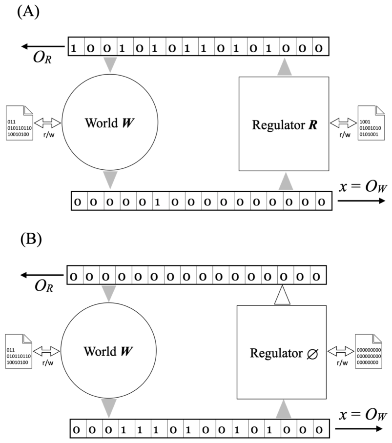
Figure 2.
Records used by the Good Algorithmic Regulator Theorem, extending the ART setup [1]. Panel A is the regulated episode; panel B is its matched null, illustrated by a fixed zero-action protocol. The initial regulator data are retained; the null suppresses its actions without assuming erasure of its private memory. The balance uses , the initial description R, actions , final private state , and complementary world record from panel A to reconstruct . The dashed region is the selected record, not the whole world state. No complementary record from panel B is supplied. The side sheets depict private data and work tapes; their displayed bits are illustrative. Each world output is a selected record of that episode. Section 5.4 treats the additional case in which it represents another world variable.
Figure 2.
Records used by the Good Algorithmic Regulator Theorem, extending the ART setup [1]. Panel A is the regulated episode; panel B is its matched null, illustrated by a fixed zero-action protocol. The initial regulator data are retained; the null suppresses its actions without assuming erasure of its private memory. The balance uses , the initial description R, actions , final private state , and complementary world record from panel A to reconstruct . The dashed region is the selected record, not the whole world state. No complementary record from panel B is supplied. The side sheets depict private data and work tapes; their displayed bits are illustrative. Each world output is a selected record of that episode. Section 5.4 treats the additional case in which it represents another world variable.
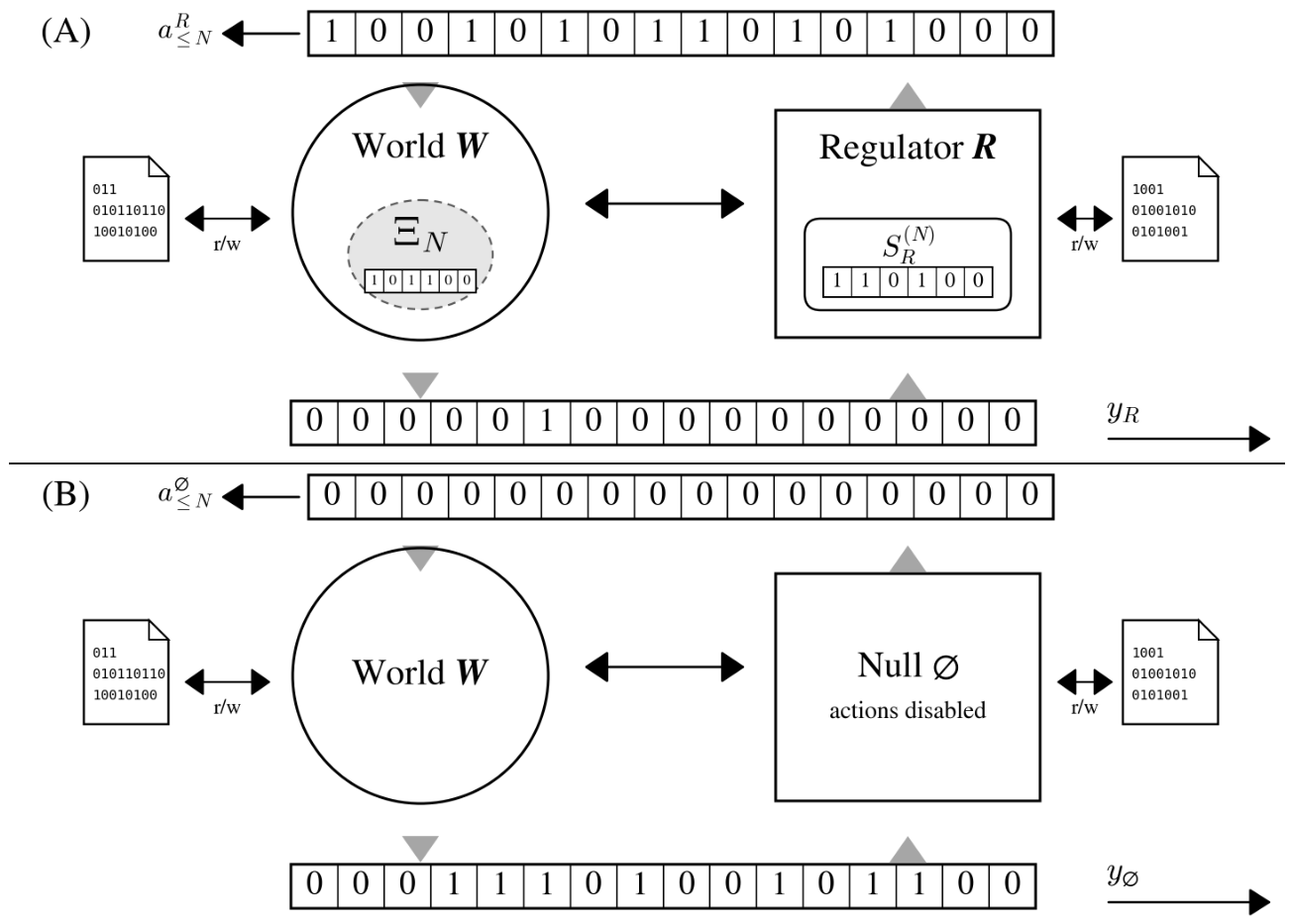
Table 1.
A gap of N bits need not imply N bits of initial shared information. Entries suppress additive coding terms; “negligible” means no larger than that allowance. The last row uses an independent incompressible key of length n, with . Every row assumes a sufficient complementary world record. The final column identifies a sufficient source of the disturbance sequence, not a unique location or causal allocation.
Table 1.
A gap of N bits need not imply N bits of initial shared information. Entries suppress additive coding terms; “negligible” means no larger than that allowance. The last row uses an independent incompressible key of length n, with . Every row assumes a sufficient complementary world record. The final column identifies a sufficient source of the disturbance sequence, not a unique location or causal allocation.
| Scenario | Initial shared information | Additional information | Record specifying d |
| Preloaded cancellation | N | Negligible | Initial regulator data |
| Online cancellation | Negligible | N | Action sequence |
| Blind clamp | Negligible | N | Complementary world record |
| Clamp with private retention | Negligible | N | Final regulator memory |
| One intervention using a short world-specific key | N | Complementary world record |
Table 2.
Regulation criteria, conditions, and world-model content. The conditions column identifies the restrictions relevant to the comparison; the cited results retain their technical hypotheses. Structural model relations and Shannon information are distinguished from the information initially shared by world and regulator, .
Table 2.
Regulation criteria, conditions, and world-model content. The conditions column identifies the restrictions relevant to the comparison; the cited results retain their technical hypotheses. Structural model relations and Shannon information are distinguished from the information initially shared by world and regulator, .
| Result | Regulation criterion | Conditions for the stated conclusion | World structure or information required |
| Ashby[5] | Keep outcomes within an acceptable set; reduce outcome variety. | Initially, distinct disturbances give distinct outcomes at fixed response; Ashby’s Sections 11/9–11/11 allow suppression by the mechanism. | A requirement on response variety. An internal world representation is not established; a fixed response can suffice under the relaxation. |
| Conant–Ashby[4] | Minimize outcome entropy for a fixed system-event distribution. | Fixed outcome map; optimization over conditional action policies. An optimal policy can be chosen deterministic. | A mapping from system events to actions, called a model. It can be constant; nontrivial retained world distinctions and shared information are not forced. |
| Francis–Wonham[18] | Exact asymptotic rejection or tracking for a specified signal class. | Closed-loop stability, all initial states, and regulation maintained under specified plant perturbations. | The controller contains the required signal-generating dynamics: shared structure with the relevant part of the world. No bound on shared information is given. |
| Sontag[17] | Exact adaptation to every input in the specified class. | Signal detection, all initial states, bounded trajectories, recurrent input generation, and the stated normal-form hypotheses. | An output-driven subsystem generates the input class. This represents external signal structure; its initial shared information is not quantified. |
| Touchette–Lloyd[19,20] | Reduce the Shannon entropy of the controlled state. | Specified sensor and actuation channels; the maximum reduction without observations is included in the bound. | Observation mutual information limits the additional gain. An internal generator is not required; the information can be acquired during control. |
| ART[1] | Reduce the complexity of a selected finite output relative to its matched null. | A specified explanation code, universal program prior, regulated output computable from the pair, and null output computable from the world. | Initial shared information enters a bound on one explanation’s posterior weight. The bound does not imply that the posterior concentrates on regulators sharing much information with the world. |
| GART, Theorem 1(this paper) | Reduce the complexity of a selected finite output relative to its matched null. | Finite strings; no prior or probability law. A fixed null-output map, a large gap, and an independently bounded residual. The episode-record form additionally requires reconstruction from the supplied records. | The initial regulator shares at least the gap minus the residual and coding overhead with the world. Equation (17) gives the identity behind the inequality. The generative example realizes this content as a model used in action. |
| Probabilistic ART, Corollary 4(this paper) | The same output comparison, under a probability law on admissible explanations. | Any law on a countable class; the observed output as evidence; GART’s bound holds on the event that the residual is at most . | Conditioned on that event, an explanation whose shared information falls k bits short of the gap has probability at most , with h the coding allowance, and probability zero once k exceeds : a conditional initial-information guarantee. |
Disclaimer/Publisher’s Note: The statements, opinions and data contained in all publications are solely those of the individual author(s) and contributor(s) and not of MDPI and/or the editor(s). MDPI and/or the editor(s) disclaim responsibility for any injury to people or property resulting from any ideas, methods, instructions or products referred to in the content. |
© 2026 by the authors. Licensee MDPI, Basel, Switzerland. This article is an open access article distributed under the terms and conditions of the Creative Commons Attribution (CC BY) license (http://creativecommons.org/licenses/by/4.0/).
Copyright: This open access article is published under a Creative Commons CC BY 4.0 license, which permit the free download, distribution, and reuse, provided that the author and preprint are cited in any reuse.