Radius of Gyration of Gaussian Bridged Rings: Derivations and Finite-Chain Corrections

1. Introduction

Joining the ends of a polymer changes its dimensions without changing its contour length. The dependence of molecular size on branching and ring closure is a classical problem in polymer statistics [1]. For Gaussian chains, the problem can be treated exactly because the connectivity imposes linear constraints on the segment vectors. The resulting correlations determine the mean-square radius of gyration.

We consider Gaussian bridged rings: f Gaussian chains joining two common junctions. This is the Gaussian-chain model of the bridged polycyclic rings studied by Zhu et al. [2], hereafter Paper I. Each complete chain between the junctions is called a bridge. The family includes the linear-chain limit $f=1$, a ring for $f=2$, and a theta-shaped chain for $f=3$. For general f, there are $f-1$ independent rings. The chains are allowed to pass through one another, and no knot type is prescribed. The model therefore describes the effect of connectivity within Gaussian chain statistics; excluded volume and restrictions on chain crossing are not included.

For equal bridges, each containing N statistical segments of mean-square length $b^2$, Paper I obtained

$${\mathcal{R}}_g^2={\displaystyle \frac{N{b}^2}{6}},g={\displaystyle \frac{{\mathcal{R}}_g^2}{{\mathcal{R}}_{g,\mathrm{linear},fN}^2}}={\displaystyle \frac{1}{f}}.$$

(1)

Here ${\mathcal{R}}_g^2=〈S_g^2〉$ denotes the mean-square radius of gyration, and g compares the network with a free linear chain of the same total contour length. These are Equations (14) and (15) of Paper I. At fixed bridge length, the mean-square size is independent of the number of bridges. This result is less evident than the reduction of the junction separation: adding bridges also changes the fluctuations of the center of mass. Both effects must be included.

Paper I used two routes to the Gaussian size. Its resistor-network calculation evaluates pair distances and their contour integrals in Equations (4)–(15). Its graph-theoretical calculation uses the inverse eigenvalues of a finite connectivity matrix, with the bead count and linear reference specified in Equations (16)–(18). The latter spectra were evaluated numerically in Paper I. Here the resistance calculation is given in full, the continuum spectrum is found analytically, and the finite inverse-eigenvalue sum is evaluated through discrete covariances and forest counts. The continuum and finite formulas are kept distinct.

Equation (12) of Paper I contains a typographical error. For two points on the same bridge, the alternate route passes through the other $f-1$ bridges in parallel. Both occurrences of $1/(f-2)$ in that equation must therefore be replaced by $1/(f-1)$. Let $u\in [0,1]$ be the contour separation of the two points divided by the bridge length N, and let $H_{\mathrm{I}}\left(u\right)$ denote their mean-square spatial separation. The corrected equation is

$${\displaystyle \frac{H_{\mathrm{I}}\left(u\right)}{N{b}^2}}={\displaystyle \frac{u[1-u+1/(f-1\left)\right]}{1+1/(f-1)}}=u-{\displaystyle \frac{f-1}{f}}{u}^2,f>1.$$

The two routes have resistances u and $1-u+1/(f-1)$ when the resistance of a complete bridge is set to unity; the fraction above is their parallel combination. The count $f-2$ instead applies to the remaining complete bridges when the two points lie on different bridges. The error is confined to the intermediate expression: the evaluated pair integrals and final size formulas reported in Paper I remain valid. Section 4 derives this corrected expression in Equation (22) and carries out both integrations in full.

Uehara and Deguchi [3] studied this architecture as a multi-theta chain. They derived pair and scattering functions for equal Gaussian walks and established independence of the mean-square size from the number of walks at fixed walk length. Comparisons between discrete formulas require the same convention for the mass assigned to shared junctions. We examine this point explicitly in Section 6.4. General Gaussian-network theory relates pair distances and molecular size to the graph Laplacian [4]. The finite equal-subdivision theorem of Cantarella et al. [5] includes the present two-junction graph; their work also gives its leading finite-chain correction. These established results are the starting point of the present analysis.

The contribution of the present analysis is to explain the physical cancellation behind the established size law, correct its original resistance derivation, and make the length and mass conventions explicit. The equal-bridge continuum law and finite equal-subdivision formula are recovered results. The calculations for unequal bridge properties and junction weights give explicit consequences for the two-junction network, including its response to weak length inequality. These are presented with their derivations and assumptions; no priority claim is made for a new general network theorem. The central distinction is between changing the Gaussian spring statistics and changing the mass distribution used to measure size.

The present scope is equilibrium size within the ideal Gaussian chain model. The excluded-volume treatment, Flory estimate, mean span, and pore partitioning discussed in Paper I concern different physical assumptions or observables and are not developed here. No simulation results or numerical estimates are needed for the analytical statements below.

We first define the model and the observable in Section 2, then develop six complementary derivations of the equal-bridge result. The covariance calculation in Section 3 separates junction motion from fluctuations within each bridge and identifies the cancellation responsible for independence from bridge number. The parallel-axis derivation in Section 3.5 expresses this cancellation through the sizes of individual bridges and the dispersion of their centers. The electrical-resistance calculation in Section 4 evaluates the mean-square distances between pairs of points. After correcting the intermediate expression in Section 4.2, the pair integrations recover Equations (14) and (15) of Paper I. We then extend the analysis to unequal bridges and different mass distributions in Section 5, and to finite bead chains in Section 6. Three further derivations are presented in the appendices. Appendix A constructs the network by closing the ends of a Gaussian star and calculates the fluctuations removed by the closure constraints. Appendix B obtains the size by summing the equilibrium variances of the normal modes. Appendix C uses counts of spanning trees and forests to obtain the exact finite-chain size and its long-chain limit. These six approaches describe the same Gaussian equilibrium measure and emphasize different aspects of the calculation. Their common basis in the connectivity operator is explained in Section 4.

2. The Gaussian Chain Model

2.1. Continuum Gaussian Network

Let the junctions be A and B. Bridge $e=1,\dots ,f$ is described by ${\mathit{r}}_e\left(s\right)\in {\mathbb{R}}^3$, with $0\le s\le N$, ${\mathit{r}}_e\left(0\right)={\mathit{r}}_{\mathrm{A}}$, and ${\mathit{r}}_e\left(N\right)={\mathit{r}}_{\mathrm{B}}$. Contour coordinate s counts statistical segments. The Gaussian chain weight is specified by the quadratic energy

$${\displaystyle \frac{\mathcal{H}}{k_{\mathrm{B}}T}}={\displaystyle \frac{3}{2b^2}}{\displaystyle \sum _{e=1}^f}{\int }_0^N{\left|{\displaystyle \frac{\mathrm{d}{\mathit{r}}_e}{\mathrm{d}s}}\right|}^2\mathrm{d}s.$$

(2)

Equation (2) is the usual continuum notation for a chain of Gaussian springs. It is understood through that discrete model; an individual continuum chain need not have an ordinary tangent at every point. Here $k_{\mathrm{B}}$ is Boltzmann’s constant and T is temperature. Bending stiffness and finite extensibility are absent. No external force is applied to the junctions, so their separation fluctuates in thermal equilibrium.

The contour mass density is the same on every bridge. The junctions have no additional point mass in this continuum model. We write

$$L=fN,q=N{b}^2,\mathit{R}={\mathit{r}}_{\mathrm{B}}-{\mathit{r}}_{\mathrm{A}},x=s/N.$$

(3)

L is total contour length in segment units, whereas q has units of length squared. We may set ${\mathit{r}}_{\mathrm{A}}=\mathbf{0}$ when calculating relative positions. For the normal-mode calculation it is more convenient to set the center of mass to zero. Translating the whole molecule changes neither pair distances nor its radius of gyration.

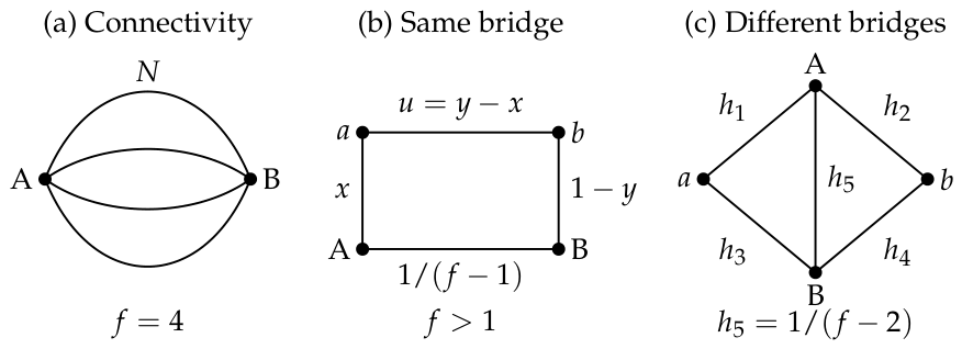
Figure 1. Connectivity and normalized electrical resistances. (a) Four equal paths share two junctions; the drawing specifies connectivity, not a spatial constraint. (b) Two points on one bridge leave $f-1$ complete bridges in the alternate route. Here $0\le x\le y\le 1$ and $u=y-x$. (c) Points on different bridges leave $f-2$ complete bridges between A and B. All resistances are divided by N. In (c), $f>2$ is understood; for $f=2$ the central edge is absent, represented by $h_5\to \infty$.

Figure 1. Connectivity and normalized electrical resistances. (a) Four equal paths share two junctions; the drawing specifies connectivity, not a spatial constraint. (b) Two points on one bridge leave $f-1$ complete bridges in the alternate route. Here $0\le x\le y\le 1$ and $u=y-x$. (c) Points on different bridges leave $f-2$ complete bridges between A and B. All resistances are divided by N. In (c), $f>2$ is understood; for $f=2$ the central edge is absent, represented by $h_5\to \infty$.

2.2. The Observable and Its Reference Chain

For a single conformation,

$$\begin{array}{cc}\hfill {\mathit{r}}_{\mathrm{cm}}& ={\displaystyle \frac{1}{L}}\sum _e{\int }_0^N{\mathit{r}}_e\left(s\right)\mathrm{d}s,\hfill \end{array}$$

(4)

$$\begin{array}{cc}\hfill S_g^2& ={\displaystyle \frac{1}{L}}\sum _e{\int }_0^N{|{\mathit{r}}_e\left(s\right)-{\mathit{r}}_{\mathrm{cm}}|}^2\mathrm{d}s\hfill \end{array}$$

(5)

$$\begin{array}{cc}\hfill & ={\displaystyle \frac{1}{2L^2}}\sum _{e,e^{\prime }}{\int }_0^N{\int }_0^N{|{\mathit{r}}_e\left(s\right)-{\mathit{r}}_{e^{\prime }}\left(t\right)|}^2\mathrm{d}s\mathrm{d}t.\hfill \end{array}$$

(6)

The factor $1/2$ compensates for ordered pairs. Ensemble averaging gives ${\mathcal{R}}_g^2$. The free continuum linear chain of contour length L has ${\mathcal{R}}_{g,\mathrm{linear},L}^2=L{b}^2/6$. The contraction factor g compares equal total contour mass and the same b.

The statement of f-independence in Equation (1) holds at fixed bridge length N. At fixed total contour length L it reads ${\mathcal{R}}_g^2=L{b}^2/\left(6f\right)$. Furthermore, $N{b}^2/6$ is the radius squared of a free linear chain of length N; it is not, for $f>1$, the gyration of one constrained bridge about that bridge’s own center of mass.

The exact finite model has N springs per bridge and $n=f(N-1)+2$ equal-mass beads, with each junction counted once. We reserve n for that bead count and L for continuum contour length. The difference is essential for finite-chain corrections (Section 6).

Throughout the continuum calculation, the freely fluctuating junction separation, uniform contour mass on each homogeneous bridge, and absence of additional junction point masses are part of the model. Neither Gaussian statistics nor a specified connectivity imposes a knot type. The results are therefore reference results for connectivity in a phantom Gaussian network, rather than exact statements about every polymer with the same chemical connectivity.

3. Junction Motion and Bridge Fluctuations

3.1. Distribution of the Junction Separation

An unconstrained Gaussian chain of N segments has endpoint density

$$G_N\left(\mathit{R}\right)={\left({\displaystyle \frac{3}{2\pi q}}\right)}^{3/2}exp\left(-{\displaystyle \frac{3R^2}{2q}}\right).$$

The bridges have common endpoints, so their endpoint weights multiply. After normalization,

$$p\left(\mathit{R}\right)={\left({\displaystyle \frac{3f}{2\pi q}}\right)}^{3/2}exp\left(-{\displaystyle \frac{3f{R}^2}{2q}}\right),〈R_{\alpha }{R}_{\beta }〉={\displaystyle \frac{q}{3f}}{\delta }_{\alpha \beta },〈R^2〉={\displaystyle \frac{q}{f}}.$$

(7)

The mean-square junction separation is reduced by a factor f relative to the end-to-end distance of one free chain. Each bridge contributes the same quadratic energy for stretching the separation.

3.2. Path Decomposition and Integrated Covariance

For a prescribed $\mathit{R}$, the mean position at contour fraction x is $x\mathit{R}$. We separate this mean path from its fluctuations:

$${\mathit{r}}_e\left(Nx\right)=x\mathit{R}+{\mathit{\eta }}_e\left(x\right),0\le x\le 1,$$

(8)

where ${\mathit{\eta }}_e\left(0\right)={\mathit{\eta }}_e\left(1\right)=\mathbf{0}$. Such a Gaussian path with both endpoints fixed is called a Brownian bridge [6].

Its covariance follows directly from the free-chain covariance. Let ${\mathit{W}}_e\left(x\right)$ be a free Gaussian path starting at the origin, with

$$〈{\mathit{W}}_e\left(x\right)·{\mathit{W}}_e\left(y\right)〉=qmin(x,y).$$

Subtracting the part proportional to its endpoint gives ${\mathit{\eta }}_e\left(x\right)={\mathit{W}}_e\left(x\right)-x{\mathit{W}}_e\left(1\right)$. Hence

$$\begin{array}{cc}\hfill 〈{\mathit{\eta }}_e\left(x\right)·{\mathit{\eta }}_e\left(y\right)〉& =q[min(x,y)-yx-xy+xy]\hfill \\ \hfill & =q[min(x,y)-xy],\hfill \\ \hfill 〈{\mathit{\eta }}_e\left(x\right)·{\mathit{W}}_e\left(1\right)〉& =q(x-x)=0.\hfill \end{array}$$

The same cancellation holds for every Cartesian covariance. Since the variables are jointly Gaussian, the bridge fluctuation is independent of the endpoint. Imposing common endpoints therefore changes only their distribution. The bridge fluctuations remain independent of $\mathit{R}$ and of one another, so

$$〈{\mathit{\eta }}_e\left(x\right)·{\mathit{\eta }}_{e^{\prime }}\left(y\right)〉={\delta }_{e{e}^{\prime }}q[min(x,y)-xy].$$

(9)

For one Cartesian component, the right-hand side is divided by three.

Define the bridge-average fluctuation ${\mathit{J}}_e={\int }_0^1{\mathit{\eta }}_e\left(x\right)\mathrm{d}x$. The elementary integrals needed below are

$${\int }_0^1{x}^2\mathrm{d}x={\displaystyle \frac{1}{3}},{\int }_0^{1}x(1-x)\mathrm{d}x={\displaystyle \frac{1}{6}}.$$

$$\begin{array}{cc}\hfill {\int }_0^1{\int }_0^1[min(x,y)-xy]\mathrm{d}x\mathrm{d}y& =2{\int }_0^1{\int }_0^{x}y(1-x)\mathrm{d}y\mathrm{d}x\hfill \\ \hfill & ={\int }_0^1{x}^2(1-x)\mathrm{d}x={\displaystyle \frac{1}{12}}.\hfill \end{array}$$

(10)

Consequently,

$$〈J_e^2〉={\displaystyle \frac{q}{12}},〈{\mathit{J}}_e·{\mathit{J}}_{e^{\prime }}〉=0(e\ne e^{\prime }),{\mathit{r}}_{\mathrm{cm}}={\displaystyle \frac{\mathit{R}}{2}}+{\displaystyle \frac{1}{f}}\sum _e{\mathit{J}}_e.$$

(11)

3.3. Subtracting the Center-of-Mass Contribution

Using $S_g^2=\overline{r^2}-r_{\mathrm{cm}}^2$, where the overbar denotes a contour-mass average, gives

$$\begin{array}{cc}\hfill \overline{〈r^2〉}& ={\int }_0^1\left[x^2〈R^2〉+qx(1-x)\right]\mathrm{d}x={\displaystyle \frac{〈R^2〉}{3}}+{\displaystyle \frac{q}{6}},\hfill \\ \hfill 〈r_{\mathrm{cm}}^2〉& ={\displaystyle \frac{〈R^2〉}{4}}+{\displaystyle \frac{1}{f^2}}\sum _e〈J_e^2〉={\displaystyle \frac{〈R^2〉}{4}}+{\displaystyle \frac{q}{12f}}.\hfill \end{array}$$

Subtracting and substituting Equation (7),

$${\mathcal{R}}_g^2={\displaystyle \frac{〈R^2〉}{12}}+{\displaystyle \frac{q}{6}}-{\displaystyle \frac{q}{12f}}={\displaystyle \frac{q}{12f}}+{\displaystyle \frac{q}{6}}-{\displaystyle \frac{q}{12f}}={\displaystyle \frac{q}{6}}.$$

(12)

The junction separation contributes $q/\left(12f\right)$ to the mean-square size. The subtraction of the fluctuating center of mass removes the same amount. The remaining term, $q/6$, comes from the fluctuations along the bridges.

Keeping the endpoints fixed instead of averaging them gives the useful conditional formula

$$〈S_g^2\mid \mathit{R}〉={\displaystyle \frac{R^2}{12}}+{\displaystyle \frac{q(2f-1)}{12f}}.$$

(13)

Thus a network whose junctions are externally held at a prescribed separation does not in general obey Equation (1). The equilibrium distribution of $\mathit{R}$ is part of the result’s assumptions.

3.4. Pointwise Pair Distances

Both contour fractions in this subsection are measured from A. For two points on the same bridge, let $u=|x-y|$. Equation (9) gives

$$〈|{\mathit{\eta }}_e\left(x\right)-{\mathit{\eta }}_e{\left(y\right)|}^2〉=q(u-u^2).$$

The common endpoint contribution adds $q{(x-y)}^2/f$, so

$$H_{\mathrm{I}}(x,y)\equiv 〈|{\mathit{r}}_e\left(Nx\right)-{\mathit{r}}_e{\left(Ny\right)|}^2〉=q\left[u-{\displaystyle \frac{f-1}{f}}{u}^2\right].$$

(14)

For points on distinct bridges the fluctuation covariance is zero:

$$H_{\mathrm{II}}(x,y)\equiv 〈|{\mathit{r}}_e\left(Nx\right)-{\mathit{r}}_{e^{\prime }}{\left(Ny\right)|}^2〉=q\left[x(1-x)+y(1-y)+{\displaystyle \frac{{(x-y)}^2}{f}}\right],e\ne e^{\prime }.$$

(15)

These pair distances will also follow from the electrical calculation in Section 4. At $x=0,y=1$, both give the junction separation $q/f$. At $x=y=0$ or $x=y=1$, the two points are at the same junction and the distance vanishes.

3.5. Physical Interpretation from the Parallel-Axis Theorem

The parallel-axis identity separates the size of each bridge from the dispersion of the bridge centers. Let ${\mathit{c}}_e={\int }_0^1{\mathit{r}}_e\left(Nx\right)\mathrm{d}x$ and $S_e^2={\int }_0^1{|{\mathit{r}}_e\left(Nx\right)-{\mathit{c}}_e|}^2\mathrm{d}x$. For equal bridge masses, the following holds for each conformation:

$$S_g^2={\displaystyle \frac{1}{f}}\sum _e{S}_e^2+{\displaystyle \frac{1}{2f^2}}\sum _{e,e^{\prime }}{|{\mathit{c}}_e-{\mathit{c}}_{e^{\prime }}|}^2.$$

(16)

To obtain it, expand ${\mathit{r}}_e-{\mathit{r}}_{\mathrm{cm}}=({\mathit{r}}_e-{\mathit{c}}_e)+({\mathit{c}}_e-{\mathit{r}}_{\mathrm{cm}})$. The cross term integrates to zero on each bridge, and the usual pair identity converts the variance of the ${\mathit{c}}_e$ into the last term.

Since ${\mathit{c}}_e=\mathit{R}/2+{\mathit{J}}_e$, the internal size of one bridge is

$$\begin{array}{cc}\hfill 〈S_e^2〉& =\left({\displaystyle \frac{〈R^2〉}{3}}+{\displaystyle \frac{q}{6}}\right)-\left({\displaystyle \frac{〈R^2〉}{4}}+{\displaystyle \frac{q}{12}}\right)\hfill \\ \hfill & ={\displaystyle \frac{〈R^2〉}{12}}+{\displaystyle \frac{q}{12}}={\displaystyle \frac{q(f+1)}{12f}}.\hfill \end{array}$$

(17)

For two different bridges,

$$〈|{\mathit{c}}_e-{\mathit{c}}_{e^{\prime }}{|}^2〉=〈|{\mathit{J}}_e-{\mathit{J}}_{e^{\prime }}{|}^2〉={\displaystyle \frac{q}{6}}.$$

There are $f(f-1)$ ordered distinct pairs of bridge centers. Hence

$${\mathcal{R}}_g^2=\underset{\mathrm{mean}\mathrm{internal}\mathrm{size}}{\underbrace{{\displaystyle \frac{q(f+1)}{12f}}}}+\underset{\mathrm{dispersion}\mathrm{of}\mathrm{centers}}{\underbrace{{\displaystyle \frac{q(f-1)}{12f}}}}={\displaystyle \frac{q}{6}}.$$

(18)

As f grows at fixed N, each constrained bridge becomes smaller about its own center while the center-dispersion contribution grows by the same amount. The two changes cancel. The size of the whole network thus equals that of a free chain of length N, even though each bridge within the network is smaller than that free chain for $f>1$.

4. Electrical Resistance and the Correction to Paper I

4.1. Why Electrical Resistance Is a Mean-Square Distance

First consider a finite network of identical Gaussian springs. Let E be the set of springs, with each spring counted once. The Boltzmann weight is

$$exp\left[-{\displaystyle \frac{3}{2b^2}}\sum _{\{i,j\}\in E}{|{\mathit{r}}_i-{\mathit{r}}_j|}^2\right].$$

(19)

After removing overall translation, fixing a pair separation and integrating the other coordinates produces a Gaussian effective energy. Its quadratic coefficient is obtained by minimizing the original quadratic form over the internal coordinates. This is the same minimization as that of electrical dissipation at fixed terminal voltage. Replace every spring by a unit resistance and let $R_{\mathrm{eff}}(i,j)$ be the resistance between beads i and j. For a prescribed separation $\mathit{d}={\mathit{r}}_i-{\mathit{r}}_j$, the minimum of the spring sum in Equation (19) is ${\left|\mathit{d}\right|}^2/R_{\mathrm{eff}}(i,j)$. Completing the square in the internal coordinates leaves an integral independent of $\mathit{d}$. Thus

$$p\left(\mathit{d}\right)\propto exp\left[-{\displaystyle \frac{{3\left|\mathit{d}\right|}^2}{2b^2{R}_{\mathrm{eff}}(i,j)}}\right].$$

Its second moment is

$$〈|{\mathit{r}}_i-{\mathit{r}}_j{|}^2〉=b^2{R}_{\mathrm{eff}}(i,j).$$

(20)

The matrix form will be useful below. Define the connectivity matrix K by taking $K_{ii}$ to be the number of springs attached to bead i and $K_{ij}$ to be minus the number joining i to j for $i\ne j$. It is the graph Laplacian. With the center of mass fixed, the covariance of one Cartesian coordinate is $b^2{K}^{+}/3$, where $K^{+}$ inverts K on vectors whose components sum to zero and is zero on the constant vector. This is the Moore–Penrose inverse. Therefore

$$R_{\mathrm{eff}}(i,j)={({\mathit{e}}_i-{\mathit{e}}_j)}^{\mathsf{T}}{K}^{+}({\mathit{e}}_i-{\mathit{e}}_j),$$

where ${\mathit{e}}_i$ is the vector with component i equal to one and all other components zero. Summing the coordinate variances again gives Equation (20) [7,8].

For n equal-mass beads, this also shows directly why the resistance and spectral calculations agree. Expanding the quadratic form gives $R_{\mathrm{eff}}(i,j)=K_{ii}^{+}+K_{jj}^{+}-2K_{ij}^{+}$. Every row of $K^{+}$ sums to zero, so

$$\sum _{i<j}{R}_{\mathrm{eff}}(i,j)=(n-1)tr{K}^{+}-2\sum _{i<j}{K}_{ij}^{+}=ntr{K}^{+}.$$

The pair definition of gyration therefore gives

$${\mathcal{R}}_g^2={\displaystyle \frac{b^2}{n^2}}\sum _{i<j}{R}_{\mathrm{eff}}(i,j)={\displaystyle \frac{b^2}{n}}tr{K}^{+}={\displaystyle \frac{b^2}{n}}{\displaystyle \sum _{p=1}^{n-1}}{\lambda }_p^{-1}.$$

(21)

The sum here is over unordered bead pairs. The covariance is the inverse of the same quadratic form whose eigenvalues enter the final expression. Appendix C expresses this trace through the coefficients of the characteristic polynomial and hence through spanning trees and forests. These are different ways of evaluating one Gaussian expectation.

A chain occupying a fraction u of one bridge has $Nu$ unit resistances in series and hence resistance $Nu$. Dividing all resistances by N therefore converts effective resistance into mean-square distance in units of $q=N{b}^2$. The familiar series and parallel laws apply to the reduced network. A general Wheatstone network additionally requires a node-equation or delta–star reduction; it is not always reducible by series and parallel operations alone.

4.2. Points on the Same Bridge: The Corrected Denominator

Use Figure 1b. Let u be the fractional contour separation of the two points on their bridge, with $0\le u\le 1$. One route between them is the direct subchain, of normalized resistance u. The other consists of the remaining portions of that same bridge, of combined resistance $1-u$, and all the other bridges between A and B. Those $f-1$ bridges in parallel have resistance $1/(f-1)$. For $f>1$,

$$\begin{array}{cc}\hfill {\displaystyle \frac{H_{\mathrm{I}}}{q}}& ={\left[{\displaystyle \frac{1}{u}}+{\displaystyle \frac{1}{1-u+1/(f-1)}}\right]}^{-1}\hfill \end{array}$$

(22)

$$\begin{array}{cc}\hfill & ={\displaystyle \frac{u[1-u+1/(f-1\left)\right]}{1+1/(f-1)}}=u-{\displaystyle \frac{f-1}{f}}{u}^2.\hfill \end{array}$$

(23)

The last expression also covers $f=1$, when there is no alternate route and $H_{\mathrm{I}}=qu$. Endpoints with zero subchain resistance are understood by continuity.

Equation (22) recovers the corrected form of Equation (12) of Paper I displayed in the Introduction. The two occurrences of $1/(f-2)$ in the original equation should be $1/(f-1)$. For $f=2$, the correct ring result is $q(u-u^2/2)$. The printed $1/(f-2)$ expression is undefined at $f=2$ as written; its limit after simplification is the incorrect result $qu$. The alternate path around the ring must be retained.

4.3. Points on Different Bridges

Use the labels of Figure 1c. Points a and b have contour fractions x and y from A. For $f>2$ the normalized resistances are

$$h_1=x,h_3=1-x,h_2=y,h_4=1-y,h_5=m={\displaystyle \frac{1}{f-2}}.$$

The two-terminal resistance is

$${\displaystyle \frac{H_{\mathrm{II}}}{q}}={\displaystyle \frac{h_5(h_1+h_2)(h_3+h_4)+h_1{h}_2(h_3+h_4)+h_3{h}_4(h_1+h_2)}{h_5(h_1+h_2+h_3+h_4)+(h_1+h_3)(h_2+h_4)}}.$$

(24)

Appendix D derives this formula, including its limiting cases. Substitution and simplification recover

$${\displaystyle \frac{H_{\mathrm{II}}}{q}}=x(1-x)+y(1-y)+{\displaystyle \frac{{(x-y)}^2}{f}},$$

in agreement with Equation (15). For $f=2$, there are no remaining full bridges; taking $m\to \infty$ in Equation (24) gives the two routes around the ring. There is no different-bridge pair when $f=1$.

4.4. The Two Pair Integrals

Define the ordered contour-pair integrals for one chosen bridge, or one chosen ordered pair of different bridges, by

$${\Sigma }_{\mathrm{I}}=N^2{\int }_0^1{\int }_0^1{H}_{\mathrm{I}}(x,y)\mathrm{d}x\mathrm{d}y,{\Sigma }_{\mathrm{II}}=N^2{\int }_0^1{\int }_0^1{H}_{\mathrm{II}}(x,y)\mathrm{d}x\mathrm{d}y.$$

(25)

They have the scaling $N^3{b}^2$; division by the squared total contour mass in Equation (4) restores units of length squared.

For any function of $u=|x-y|$, the square integral is $2{\int }_0^1(1-u)(\dots )\mathrm{d}u$. Thus

$$\begin{array}{cc}\hfill {\displaystyle \frac{{\Sigma }_{\mathrm{I}}}{N^3{b}^2}}& =2{\int }_0^1(1-u)\left[u-{\displaystyle \frac{f-1}{f}}{u}^2\right]\mathrm{d}u\hfill \end{array}$$

(26)

$$\begin{array}{cc}\hfill & =2\left[\left({\displaystyle \frac{1}{2}}-{\displaystyle \frac{1}{3}}\right)-{\displaystyle \frac{f-1}{f}}\left({\displaystyle \frac{1}{3}}-{\displaystyle \frac{1}{4}}\right)\right]={\displaystyle \frac{f+1}{6f}}.\hfill \end{array}$$

(27)

For distinct bridges,

$$\begin{array}{cc}\hfill {\displaystyle \frac{{\Sigma }_{\mathrm{II}}}{N^3{b}^2}}& ={\int }_0^1{\int }_0^1\left[x(1-x)+y(1-y)+{\displaystyle \frac{{(x-y)}^2}{f}}\right]\mathrm{d}x\mathrm{d}y\hfill \end{array}$$

(28)

$$\begin{array}{cc}\hfill & ={\displaystyle \frac{1}{6}}+{\displaystyle \frac{1}{6}}+{\displaystyle \frac{1}{f}}\left({\displaystyle \frac{1}{3}}+{\displaystyle \frac{1}{3}}-2·{\displaystyle \frac{1}{4}}\right)={\displaystyle \frac{2f+1}{6f}}.\hfill \end{array}$$

(29)

These are the evaluated same- and different-bridge integrals used in Paper I. Appendix E reproduces the different-bridge integral in that paper’s oppositely oriented coordinates, including the Jacobian and the integration domain.

4.5. Recovering Equations (14) and (15) of Paper I

There are f same-bridge terms and $f(f-1)$ ordered different-bridge terms. The explicit assembly is

$$\begin{array}{cc}\hfill {\mathcal{R}}_g^2& ={\displaystyle \frac{f{\Sigma }_{\mathrm{I}}+f(f-1){\Sigma }_{\mathrm{II}}}{2{\left(fN\right)}^2}}\hfill \end{array}$$

(30)

$$\begin{array}{cc}\hfill & ={\displaystyle \frac{N{b}^2}{12f^2}}\left[(f+1)+(f-1)(2f+1)\right]\hfill \end{array}$$

(31)

$$\begin{array}{cc}\hfill & ={\displaystyle \frac{N{b}^2}{12f^2}}\left(2f^2\right)={\displaystyle \frac{N{b}^2}{6}}.\hfill \end{array}$$

(32)

For $f=1$ the distinct-bridge contribution is omitted and the same result follows from ${\Sigma }_{\mathrm{I}}$. Division by the continuum reference chain of length $fN$ gives

$$g={\displaystyle \frac{N{b}^2/6}{fN{b}^2/6}}={\displaystyle \frac{1}{f}}.$$

(33)

The correction is therefore local to the same-bridge intermediate expression; the final formulas being recovered are unchanged.

5. Unequal Bridges and Mass Weighting

5.1. Common Statistical Segment Length

Now let bridge e contain $N_e>0$ segment units, let b be common, and write $L={\sum }_e{N}_e$. Assume the same mass per statistical segment, so the bridge mass fractions are $w_e=N_e/L$. Multiplying endpoint propagators gives

$$Q_R\equiv 〈R^2〉={\displaystyle \frac{b^2}{{\sum }_e{N}_e^{-1}}}.$$

(34)

The independent bridge fluctuations have $〈J_e^2〉=N_e{b}^2/12$. Because every mean path is $x\mathit{R}$ when expressed in its own fractional coordinate,

$$\begin{array}{cc}\hfill \overline{〈r^2〉}& ={\displaystyle \frac{Q_R}{3}}+{\displaystyle \frac{b^2}{6L}}\sum _e{N}_e^2,\hfill \\ \hfill 〈r_{\mathrm{cm}}^2〉& ={\displaystyle \frac{Q_R}{4}}+{\displaystyle \frac{b^2}{12L^2}}\sum _e{N}_e^3.\hfill \end{array}$$

Consequently,

$${\mathcal{R}}_g^2={\displaystyle \frac{b^2}{12{\sum }_e{N}_e^{-1}}}+{\displaystyle \frac{b^2}{6L}}\sum _e{N}_e^2-{\displaystyle \frac{b^2}{12L^2}}\sum _e{N}_e^3.$$

(35)

This formula has been obtained directly from the bridge covariance. It is consistent with the general covariance and resistance description of Gaussian networks [4]; no equal-subdivision theorem is needed for the unequal lengths used here. Its contraction factor, with the same uniform segment mass and common b, is

$$g={\displaystyle \frac{1}{2L{\sum }_e{N}_e^{-1}}}+{\displaystyle \frac{{\sum }_e{N}_e^2}{L^2}}-{\displaystyle \frac{{\sum }_e{N}_e^3}{2L^3}}.$$

(36)

It reduces to $1/f$ when all $N_e$ are equal. For $f=1$, it gives ${\mathcal{R}}_g^2=N_1{b}^2/6$. For $f=2$, writing $a=N_1$, $c=N_2$ gives

$${\displaystyle \frac{{\mathcal{R}}_g^2}{b^2}}={\displaystyle \frac{ac}{12(a+c)}}+{\displaystyle \frac{a^2+c^2}{6(a+c)}}-{\displaystyle \frac{a^3+c^3}{12{(a+c)}^2}}={\displaystyle \frac{a+c}{12}}.$$

Thus splitting a uniform ring into two arbitrarily labeled arcs does not change its size. For $f\ge 3$ the individual bridge lengths generally matter.

5.2. Small Differences Between Bridge Lengths

Equation (36) gives the response to a redistribution of contour length without requiring a separate model. Keep f and L fixed and write

$$N_e={\displaystyle \frac{L}{f}}(1+{\epsilon }_e),\sum _e{\epsilon }_e=0,\rho =\underset{e}{max}\left|{\epsilon }_e\right|\ll 1.$$

(37)

Let $S_k={\sum }_e{\epsilon }_e^k$. The three terms in Equation (36) can be expanded separately:

$$\begin{array}{cc}\hfill {\displaystyle \frac{1}{2L{\sum }_e{N}_e^{-1}}}& ={\displaystyle \frac{1}{2f(f+S_2-S_3+O\left({\rho }^4\right))}}={\displaystyle \frac{1}{2f^2}}-{\displaystyle \frac{S_2-S_3}{2f^3}}+O\left({\rho }^4\right),\hfill \\ \hfill {\displaystyle \frac{{\sum }_e{N}_e^2}{L^2}}& ={\displaystyle \frac{f+S_2}{f^2}},\hfill \\ \hfill {\displaystyle \frac{{\sum }_e{N}_e^3}{2L^3}}& ={\displaystyle \frac{f+3S_2+S_3}{2f^3}}.\hfill \end{array}$$

The terms linear in the length changes vanish because total length is fixed, and the cubic terms cancel. Thus

$$g={\displaystyle \frac{1}{f}}+{\displaystyle \frac{f-2}{f^3}}\sum _e{\epsilon }_e^2+O\left({\rho }^4\right).$$

(38)

For $f>2$, equal lengths give a strict local minimum of g under small redistributions of contour length. This is a local statement, not a claim about all possible length distributions. For $f=2$, the exact ring result makes $g=1/2$ for every division into two arcs.

5.3. Different Gaussian Variances and Masses

We can also allow the statistical segment length and the mass per segment to differ between bridges. Suppose bridge e is homogeneous along its own contour but has free end-to-end variance $q_e=N_e{b}_e^2$ and mass fraction $w_e>0$, with ${\sum }_e{w}_e=1$. Uniform mass density within each bridge is assumed; $w_e$ need not equal $N_e/\sum N_e$. Then

$$Q_R={\left(\sum _e{q}_e^{-1}\right)}^{-1},〈J_e^2〉={\displaystyle \frac{q_e}{12}},$$

where ${\mathit{J}}_e={\int }_0^1{\mathit{\eta }}_e\left(x\right)\mathrm{d}x$ and the fluctuation covariance is $q_e[min(x,y)-xy]$ on bridge e. There are no additional junction point masses in this continuum observable. With A at the origin,

$${\mathit{r}}_{\mathrm{cm}}=\sum _e{w}_e{\int }_0^1{\mathit{r}}_e\left(N_{e}x\right)\mathrm{d}x={\displaystyle \frac{\mathit{R}}{2}}+\sum _e{w}_e{\mathit{J}}_e.$$

Independence of the bridge fluctuations and of $\mathit{R}$ gives

$$\begin{array}{cc}\hfill \overline{〈r^2〉}& ={\displaystyle \frac{Q_R}{3}}+{\displaystyle \frac{1}{6}}\sum _e{w}_e{q}_e,\hfill \\ \hfill 〈r_{\mathrm{cm}}^2〉& ={\displaystyle \frac{Q_R}{4}}+{\displaystyle \frac{1}{12}}\sum _e{w}_e^2{q}_e.\hfill \end{array}$$

(39)

The first average weights each bridge once; the second squares its weight because the center of mass is an average of the positions. Subtracting yields

$${\mathcal{R}}_g^2={\displaystyle \frac{Q_R}{12}}+{\displaystyle \frac{1}{6}}\sum _e{w}_e{q}_e-{\displaystyle \frac{1}{12}}\sum _e{w}_e^2{q}_e.$$

(40)

The first term is set by the junction separation. The second is the mass average of the bridge fluctuations, and the last subtracts their contribution to the motion of the center of mass. Using $w_e=N_e/L$ and common b recovers Equation (35). When the segment lengths or segment masses differ, a contraction factor is defined only after specifying the linear reference, its mass distribution, and its segment variances.

For equal $q_e=q$ but arbitrary bridge mass fractions, the same result has the particularly simple form

$${\mathcal{R}}_g^2={\displaystyle \frac{q}{6}}-{\displaystyle \frac{q}{12}}\sum _e{\left(w_e-{\displaystyle \frac{1}{f}}\right)}^2.$$

(41)

Changing the mass weighting at fixed spring statistics therefore has a different effect from redistributing contour length with a common mass per segment. In the former case, the configuration measure is unchanged; only the observable and its center of mass are changed.

If the Gaussian segment variance varies within a bridge, its conditional mean need not be linear in the original contour coordinate, and its covariance must be obtained with that varying variance. Variation of mass density alone leaves the configurational covariance unchanged but changes the contour averages. In either case the actual mass distribution must be used in the definition of the observable. The chains remain Gaussian and are allowed to cross.

6. Exact Finite Bead-Spring Chains

6.1. Closed Formula and Bead-Count Convention

Let $N\ge 1$ be an integer and $f\ge 1$. Every bridge has N identical Gaussian springs. There are $N-1$ interior beads per bridge and two shared junction beads, all with the same mass:

$$n=f(N-1)+2.$$

(42)

The $fN$ springs and the n beads are different counts. In particular, a linear reference with the same total mass and the same mass per bead has n beads and $n-1$ springs. This is the convention of Equations (16)–(18) of Paper I, with its $N_t$ equal to our n. The formula below is an analytical evaluation of the static spectral sum used for the finite-chain comparison in Figure 3 of that paper. The derivation uses the finite Gaussian measure directly and requires no numerical eigenvalues.

The finite corrections describe discrete mass averaging and the counting of shared junctions within this specified Gaussian spring model. They do not include the bending stiffness, finite extensibility, or excluded-volume effects that can also matter for short real chains.

The exact mean-square size is

$$\begin{array}{cc}\hfill {\displaystyle \frac{{\mathcal{R}}_g^2(N,f)}{b^2}}& ={\displaystyle \frac{N}{4f}}-{\displaystyle \frac{N(N^2-1)}{12n^2}}+{\displaystyle \frac{(f-1)(N^2-1)(2n-N)}{12n^2}}\hfill \\ \hfill & ={\displaystyle \frac{N}{4f}}+{\displaystyle \frac{(N^2-1)[2(f-1)n-fN]}{12n^2}}.\hfill \end{array}$$

(43)

This compact expression is equivalent to the expanded formula

$$\begin{array}{cc}\hfill {\displaystyle \frac{{\mathcal{R}}_g^2(N,f)}{b^2}}& ={\displaystyle \frac{\mathcal{P}(N,f)}{6f{n}^2}},\hfill \\ \hfill \mathcal{P}(N,f)& =N^3{f}^3-N^{2}f(f^2-4)-N(f^3-3f^2+6f-6)+f(f-1)(f-2).\hfill \end{array}$$

(44)

The covariance derivation below establishes this expression directly. Appendix C gives a derivation by counting forests. It is also the two-junction specialization of Theorem 2 of Cantarella et al. [5]. Appendix F shows that reduction and distinguishes the theorem from a misprint in the polynomial displayed in their multi-theta example.

6.2. Derivation from Discrete Bridge Covariances

Index interior beads on a bridge by $j=1,\dots ,N-1$. With A fixed at the origin and B at $\mathit{R}$,

$${\mathit{r}}_{e,j}={\displaystyle \frac{j}{N}}\mathit{R}+{\mathit{\eta }}_{e,j},〈{\mathit{\eta }}_{e,j}·{\mathit{\eta }}_{e^{\prime },k}〉={\delta }_{e{e}^{\prime }}{b}^2\left[min(j,k)-{\displaystyle \frac{jk}{N}}\right],〈R^2〉={\displaystyle \frac{N{b}^2}{f}}.$$

(45)

The endpoint weight is unchanged by counting junction mass in the observable; the mass affects the center of mass, not this configurational Gaussian measure.

The coefficient of $\mathit{R}$ in the sum over all bead positions is $1+f{\sum }_{j=1}^{N-1}j/N=1+f(N-1)/2=n/2$. Hence

$${\mathit{r}}_{\mathrm{cm}}={\displaystyle \frac{\mathit{R}}{2}}+{\displaystyle \frac{1}{n}}\sum _e{\displaystyle \sum _{j=1}^{N-1}}{\mathit{\eta }}_{e,j}.$$

The required finite sums are

$$\begin{array}{cc}\hfill {\displaystyle \sum _{j=1}^{N-1}}{\displaystyle \frac{j^2}{N^2}}& ={\displaystyle \frac{(N-1)(2N-1)}{6N}},\hfill \\ \hfill {\displaystyle \sum _{j=1}^{N-1}}\left(j-{\displaystyle \frac{j^2}{N}}\right)& ={\displaystyle \frac{N^2-1}{6}},\hfill \\ \hfill {\displaystyle \sum _{j,k=1}^{N-1}}\left[min(j,k)-{\displaystyle \frac{jk}{N}}\right]& ={\displaystyle \frac{N(N^2-1)}{12}}.\hfill \end{array}$$

(46)

For the last identity, ${\sum }_{j,k}min(j,k)={\sum }_{r=1}^{N-1}{(N-r)}^2=N(N-1)(2N-1)/6$, and $N^{-1}{\left({\sum }_{j}j\right)}^2=N{(N-1)}^2/4$; their difference gives the stated result.

Including B once in the squared-position sum and A once with zero position,

$$\begin{array}{cc}\hfill {\displaystyle \frac{1}{n}}\sum _i〈r_i^2〉& ={\displaystyle \frac{〈R^2〉}{n}}\left[1+{\displaystyle \frac{f(N-1)(2N-1)}{6N}}\right]+{\displaystyle \frac{f{b}^2(N^2-1)}{6n}},\hfill \\ \hfill 〈r_{\mathrm{cm}}^2〉& ={\displaystyle \frac{〈R^2〉}{4}}+{\displaystyle \frac{f{b}^{2}N(N^2-1)}{12n^2}}.\hfill \end{array}$$

Subtracting yields

$${\displaystyle \frac{{\mathcal{R}}_g^2}{b^2}}={\displaystyle \frac{N}{f}}\left\{{\displaystyle \frac{1}{n}}\left[1+{\displaystyle \frac{f(N-1)(2N-1)}{6N}}\right]-{\displaystyle \frac{1}{4}}\right\}+{\displaystyle \frac{f(N^2-1)}{6n}}-{\displaystyle \frac{fN(N^2-1)}{12n^2}}.$$

(47)

Substitution of $n=f(N-1)+2$ reduces Equation (47) to Equation (43). This proves the finite result without a spectral sum or a combinatorial enumeration.

6.3. Contraction Factor and Limiting Cases

A free linear chain of n equal-mass beads has pair distances $b^2|i-j|$. Its exact radius is

$${\mathcal{R}}_{g,\mathrm{linear},n}^2={\displaystyle \frac{b^2}{n^2}}{\displaystyle \sum _{k=1}^{n-1}}(n-k)k={\displaystyle \frac{b^2(n^2-1)}{6n}}.$$

(48)

Thus

$$g(N,f)={\displaystyle \frac{\mathcal{P}(N,f)}{f(n-1)n(n+1)}}.$$

(49)

Subtracting the continuum contraction factor and factoring the numerator gives

$$g(N,f)-{\displaystyle \frac{1}{f}}={\displaystyle \frac{(N-1)(f-1)(f-2)(2n-1)}{f(n-1)n(n+1)}}.$$

(50)

For $f>2$ and $N>1$, every factor on the right-hand side is positive. Thus the finite-chain contraction factor lies strictly above $1/f$. At $N=1$ it equals $1/f$, and it returns to that value as $N\to \infty$. Its dependence on the integer subdivision number therefore cannot be monotone over the full range $N\ge 1$. This conclusion follows from the exact factorization, without a plot or an eigenvalue calculation.

The remaining limiting cases are:

• For $f=1$, the graph is a linear chain with $n=N+1$: ${\mathcal{R}}_g^2=b^{2}N(N+2)/\left[6(N+1)\right]$ and $g=1$.
• For $f=2$, the graph is a ring with $n=2N$: ${\mathcal{R}}_g^2=b^2(4N^2-1)/\left(24N\right)$ and $g=1/2$ for every N. The $N=1$ case is the two-vertex multigraph with two parallel springs.
• For $N=1$, there are only two beads joined by f parallel springs: $〈R^2〉=b^2/f$, ${\mathcal{R}}_g^2=b^2/\left(4f\right)$, and $g=1/f$.

The continuum ring value is consistent with the classical Gaussian-ring result [9].

At fixed f, expansion of the exact formulas gives

$$\begin{array}{cc}\hfill {\displaystyle \frac{{\mathcal{R}}_g^2(N,f)}{N{b}^2}}& ={\displaystyle \frac{1}{6}}\left[1+{\displaystyle \frac{{(f-2)}^2}{f^{2}N}}+O\left(N^{-2}\right)\right],\hfill \\ \hfill g(N,f)& ={\displaystyle \frac{1}{f}}+{\displaystyle \frac{2(f-1)(f-2)}{f^{3}N}}+O\left(N^{-2}\right).\hfill \end{array}$$

(51)

The leading correction to the mean-square size vanishes for the ring, whereas the correction to g vanishes for both the linear chain and the ring. These statements use equal bead masses, with each shared junction counted once.

6.4. Junction Masses and the Meaning of Exact Independence

The equal-bead result uses a particular mass distribution. To separate that choice from the configuration measure, assign mass one to every interior bead and masses ${\mu }_{\mathrm{A}},{\mu }_{\mathrm{B}}\ge 0$ to the junctions. The total mass and the coefficient of $\mathit{R}$ in the center of mass are

$$M=f(N-1)+{\mu }_{\mathrm{A}}+{\mu }_{\mathrm{B}}>0,c_R={\displaystyle \frac{{\mu }_{\mathrm{B}}+f(N-1)/2}{M}}.$$

(52)

The Gaussian measure and $〈R^2〉=N{b}^2/f$ are unchanged. The mass-weighted squared-position average and center-of-mass variance follow from the same finite sums as above:

$$\begin{array}{cc}\hfill \overline{〈r^2〉}& ={\displaystyle \frac{N{b}^2}{fM}}\left[{\mu }_{\mathrm{B}}+{\displaystyle \frac{f(N-1)(2N-1)}{6N}}\right]+{\displaystyle \frac{f{b}^2(N^2-1)}{6M}},\hfill \end{array}$$

(53)

$$\begin{array}{cc}\hfill 〈r_{\mathrm{cm}}^2〉& ={\displaystyle \frac{N{b}^2}{f}}{c}_R^2+{\displaystyle \frac{f{b}^{2}N(N^2-1)}{12M^2}}.\hfill \end{array}$$

(54)

Their difference is

$$\begin{array}{cc}\hfill {\displaystyle \frac{{\mathcal{R}}_g^2}{b^2}}=& {\displaystyle \frac{N}{f}}\left\{{\displaystyle \frac{{\mu }_{\mathrm{B}}+f(N-1)(2N-1)/\left(6N\right)}{M}}-c_R^2\right\}\hfill \\ \hfill & +{\displaystyle \frac{f(N^2-1)}{6M}}-{\displaystyle \frac{fN(N^2-1)}{12M^2}}.\hfill \end{array}$$

(55)

Setting both junction masses to one recovers Equation (43). Here mass changes the gyration observable, not the spring energy or the endpoint distribution.

An instructive alternative counts the positions $j=1,\dots ,N$ once for each bridge. Then A is unweighted and the common endpoint B has weight f: ${\mu }_{\mathrm{A}}=0$, ${\mu }_{\mathrm{B}}=f$, and $M=fN$. The weighted center of mass has $c_R=(N+1)/\left(2N\right)$. Explicitly,

$$\begin{array}{cc}\hfill \overline{〈r^2〉}& ={\displaystyle \frac{b^2(N+1)(2N+1)}{6fN}}+{\displaystyle \frac{b^2(N^2-1)}{6N}},\hfill \\ \hfill 〈r_{\mathrm{cm}}^2〉& ={\displaystyle \frac{b^2{(N+1)}^2}{4fN}}+{\displaystyle \frac{b^2(N^2-1)}{12fN}}.\hfill \end{array}$$

The numerator of the difference between the terms proportional to $1/f$ is

$$2(N+1)(2N+1)-3{(N+1)}^2-(N^2-1)=0.$$

Consequently,

$${\mathcal{R}}_{g,\mathrm{one}\mathrm{end}}^2={\displaystyle \frac{b^2(N^2-1)}{6N}}.$$

(56)

This is independent of f at every N and equals the size of a free linear chain of N unit-mass beads. The convention specifies a weighted observable on the same network; it does not introduce additional physical junction beads. Interchanging A and B gives the same size.

To show that the distribution of junction mass matters, keep their combined mass equal to f and set ${\mu }_{\mathrm{A}}=fa$, ${\mu }_{\mathrm{B}}=f(1-a)$, with $0\le a\le 1$. Substitution into Equation (55) gives

$${\mathcal{R}}_g^2={\displaystyle \frac{b^2(N^2-1)}{6N}}+{\displaystyle \frac{b^{2}a(1-a)}{fN}}.$$

(57)

For a fixed mass fraction a, the additional term vanishes only when all junction mass is assigned to one end. An equal split gives the additional contribution $b^2/\left(4fN\right)$.

Independence of the mean-square size from f must also be distinguished from a finite-chain contraction factor equal to $1/f$. If the reference for Equation (56) is a free linear chain of $fN$ unit-mass beads, so that total mass is the same, then

$$g_{\mathrm{one}\mathrm{end}}={\displaystyle \frac{f(N^2-1)}{f^2{N}^2-1}},g_{\mathrm{one}\mathrm{end}}-{\displaystyle \frac{1}{f}}=-{\displaystyle \frac{f^2-1}{f(f^2{N}^2-1)}}.$$

(58)

Here $fN>1$ is required for a nonzero reference radius. For $f>1$ this ratio tends to $1/f$ only in the long-chain limit. Thus the mass convention can remove the f-dependence of the size without removing finite-chain corrections to the contraction factor. These examples make explicit the observable conventions needed when comparing discrete versions of bridge-number independence, including the multi-theta results of Uehara and Deguchi [3].

7. Conclusions

For Gaussian bridged rings with equal bridges and freely fluctuating junctions, the continuum mean-square radius of gyration is $N{b}^2/6$. The contraction factor relative to a linear chain of the same total contour mass is $1/f$. This established result follows directly when the junction separation and the fluctuations within each bridge are separated. The contribution from the junction separation is cancelled by the corresponding subtraction for the fluctuating center of mass. The parallel-axis form expresses the same cancellation as a balance between the internal size of the bridges and the dispersion of their centers.

The resistance calculation supplies the complete pair integrations behind Equations (14) and (15) of Paper I. It replaces $f-2$ by $f-1$ in the same-bridge expression while retaining $f-2$ in the different-bridge reduction. The final size and contraction formulas of Paper I are unchanged. The additional derivations in the appendices connect this calculation to star closure, the spectrum of the continuum operator, and counts of spanning forests.

Unequal bridge lengths change both the junction variance and the mass averages of the bridge fluctuations. At fixed total contour length, weak length inequality increases the contraction factor to quadratic order for more than two bridges. A redistribution of mass at fixed Gaussian spring statistics is a different operation and changes only the observable. The explicit formulas keep these effects separate.

For finite chains, the size formula with each junction counted once agrees with the general equal-subdivision theorem and gives the exact evaluation of the static spectral sum used in Paper I. The factored difference from the continuum contraction factor fixes the sign of the finite correction and establishes nonmonotonic dependence over the full subdivision range for more than two bridges. Alternative junction weights can make the mean-square size exactly independent of the number of bridges, but the contraction factor still depends on its finite linear reference. The distinction disappears at leading order in the long-chain limit. All these statements concern the specified Gaussian equilibrium measure and mass distribution, with unrestricted chain crossing.

Appendix A.1. The Size of the Unconstrained Star

Take f independent Brownian arms of contour length N with their common origin at A. Their endpoints ${\mathit{R}}_e$ satisfy $〈R_e^2〉=q$. The mean-square position averaged along any arm is ${\int }_0^{1}qx\mathrm{d}x=q/2$. An arm’s mean position has variance

$$q{\int }_0^1{\int }_0^{1}min(x,y)\mathrm{d}x\mathrm{d}y={\displaystyle \frac{q}{3}}.$$

Independence of different arms therefore gives

$${\mathcal{R}}_{g,\mathrm{star}}^2={\displaystyle \frac{q}{2}}-{\displaystyle \frac{q}{3f}}={\displaystyle \frac{q(3f-2)}{6f}},g_{\mathrm{star}}={\displaystyle \frac{3f-2}{f^2}},$$

(A1)

the classical equal-arm result [1].

Appendix A.2. The Change in Size on Closing the Star

Write the free arm as ${\mathit{W}}_e\left(x\right)=x{\mathit{R}}_e+{\mathit{\eta }}_e\left(x\right)$, where its endpoint ${\mathit{R}}_e$ is independent of the fluctuation ${\mathit{\eta }}_e$. To form the bridged network, impose ${\mathit{R}}_e={\mathit{R}}_1$ for $e=2,\dots ,f$. Define the mean endpoint and its deviations by

$$\overline{\mathit{R}}={\displaystyle \frac{1}{f}}\sum _e{\mathit{R}}_e,{\Delta }_e={\mathit{R}}_e-\overline{\mathit{R}},\sum _e{\Delta }_e=\mathbf{0}.$$

The independent, equal-variance Gaussian endpoints give

$$〈|\overline{\mathit{R}}{|}^2〉={\displaystyle \frac{q}{f}},〈{\Delta }_e^2〉=q\left(1-{\displaystyle \frac{1}{f}}\right),〈\overline{\mathit{R}}·{\Delta }_e〉=0.$$

Thus $\overline{\mathit{R}}$ is independent of all the ${\Delta }_e$. The free-star path separates into two independent parts:

$${\mathit{W}}_e\left(x\right)=\underset{{\mathit{r}}_e^c\left(x\right)}{\underbrace{x\overline{\mathit{R}}+{\mathit{\eta }}_e\left(x\right)}}+\underset{{\mathit{u}}_e\left(x\right)}{\underbrace{x{\Delta }_e}}.$$

(A2)

The first part has common endpoints and exactly the distribution of the bridged network. The second part describes the endpoint differences removed on closure. Conditioning the endpoints to coincide sets this second part to zero and leaves the first part unchanged.

The squared radius of gyration is a quadratic function of the positions. The two parts in Equation (A2) have zero mean and are independent, so their cross term has zero average. Consequently,

$${\mathcal{R}}_{g,\mathrm{star}}^2={\mathcal{R}}_{g,\mathrm{bridged}}^2+〈S_g^2\left[\mathit{u}\right]〉.$$

(A3)

The center of mass of $\mathit{u}$ is zero because ${\sum }_e{\Delta }_e=\mathbf{0}$. Its contribution to the gyration is therefore

$$〈S_g^2\left[\mathit{u}\right]〉={\displaystyle \frac{1}{f}}\sum _e{\int }_0^1{x}^2〈{\Delta }_e^2〉\mathrm{d}x={\displaystyle \frac{q}{3}}\left(1-{\displaystyle \frac{1}{f}}\right).$$

Subtracting this from Equation (A1) gives

$${\mathcal{R}}_{g,\mathrm{bridged}}^2=\left({\displaystyle \frac{q}{2}}-{\displaystyle \frac{q}{3f}}\right)-{\displaystyle \frac{q}{3}}\left(1-{\displaystyle \frac{1}{f}}\right)={\displaystyle \frac{q}{6}}.$$

(A4)

For $f=1$ there is no closure constraint; for $f=2$ the two arms form a ring. This calculation uses continuous contour mass, for which a single endpoint has zero mass. Identifying discrete end beads also changes the mass counting, as discussed in Section 6.

Appendix B.1. From Gaussian Covariance to a Spectral Trace

For the finite graph in Equation (19), choose the origin at the center of mass, so ${\sum }_i{\mathit{r}}_i=\mathbf{0}$. Diagonalizing K gives one translational zero eigenvalue and $n-1$ positive eigenvalues. Each Cartesian normal coordinate with eigenvalue ${\lambda }_p$ has variance $b^2/\left(3{\lambda }_p\right)$. Therefore

$${\mathcal{R}}_g^2={\displaystyle \frac{b^2}{n}}tr{K}^{+}={\displaystyle \frac{b^2}{n}}{\displaystyle \sum _{p=1}^{n-1}}{\displaystyle \frac{1}{{\lambda }_p}}.$$

(A5)

This graph formulation of Gaussian molecular statistics is well established [4,7,10,11]. Equation (A5) is Equation (16) of Paper I in the notation $N_t=n$. Its “Zimm matrix” is the connectivity matrix K defined in Section 4. Equation (19) of Paper I uses the eigenvalues for relaxation times; that dynamical relation is not needed for the equilibrium size. Section 6 evaluates the static sum in closed form through discrete bridge covariances, and Appendix C does so through forest counts.

In the continuum, the modes are functions along the bridges. Their normalization uses the contour integral ${\sum }_e{\int }_0^N{\varphi }_e\left(s\right){\psi }_e\left(s\right)\mathrm{d}s$. The connectivity matrix is replaced by the operator $-{\mathrm{d}}^2/\mathrm{d}{s}^2$. At each junction, all bridges have the same displacement and the sum of their outward derivatives vanishes. They are the natural boundary conditions of the Gaussian quadratic form with no additional vertex term [12]. For smooth functions $\varphi$ and $\psi$ that are continuous at the junctions, integration by parts gives

$$\sum _e{\int }_0^N{\varphi }_e^{\prime }\left(s\right){\psi }_e^{\prime }\left(s\right)\mathrm{d}s=\sum _e{\int }_0^N[-{\varphi }_e^{\prime \prime }\left(s\right)]{\psi }_e\left(s\right)\mathrm{d}s+\sum _e[{\varphi }_e^{\prime }\left(N\right){\psi }_e\left(N\right)-{\varphi }_e^{\prime }\left(0\right){\psi }_e\left(0\right)].$$

The two common junction values of $\psi$ can be varied independently. The boundary term therefore vanishes when ${\sum }_e{\varphi }_e^{\prime }\left(0\right)={\sum }_e{\varphi }_e^{\prime }\left(N\right)=0$, equivalently when the sum of outward derivatives at each junction vanishes. These conditions apply to the operator eigenfunctions. They do not require an individual Brownian conformation to have ordinary tangents or to satisfy instantaneous mechanical force balance.

To see the normalization explicitly, expand each Cartesian coordinate in modes normalized to unit contour integral. A mode of eigenvalue $\lambda$ contributes $3\lambda a^2/\left(2b^2\right)$ to the energy in units of $k_{\mathrm{B}}T$, so $〈a^2〉=b^2/\left(3\lambda \right)$. Summing the three Cartesian contributions and dividing by $L=fN$ gives

$${\mathcal{R}}_g^2={\displaystyle \frac{b^2}{L}}\sum _{\lambda >0}{\displaystyle \frac{m_{\lambda }}{\lambda }},$$

(A6)

where $m_{\lambda }$ is the number of independent modes with that eigenvalue. The constant mode translates the molecule and is omitted. The continuum modes differ from the modes of a finite bead chain; Equation (A5) must be used for that finite model.

Appendix B.2. Eigenvalues and Their Multiplicities

On edge e, a positive-eigenvalue solution has the form ${\varphi }_e\left(s\right)=a_{e}cos\left(ks\right)+d_{e}sin\left(ks\right)$. At A, the continuity and derivative conditions require

$$a_e=a\mathrm{for}\mathrm{all}e,\sum _e{d}_e=0.$$

At B, the derivative condition reduces to $-fasin\left(kN\right)+cos\left(kN\right){\sum }_e{d}_e=0$. If $sin\left(kN\right)\ne 0$, continuity at B makes all the $d_e$ equal; their sum then forces them to vanish, and the remaining derivative condition forces $a=0$. There is no nonzero eigenfunction in that case. Consequently,

$$k_p={\displaystyle \frac{p\pi }{N}},{\lambda }_p={\left({\displaystyle \frac{p\pi }{N}}\right)}^2,p=1,2,\dots .$$

(A7)

At each such p, one cosine mode common to all bridges and $f-1$ sine modes whose amplitudes sum to zero are allowed. More explicitly, take orthonormal vectors ${\mathit{v}}^{\left(\alpha \right)}\in {\mathbb{R}}^f$ with ${\sum }_e{v}_e^{\left(\alpha \right)}=0$. An orthonormal basis for the eigenspace is

$${\varphi }_{p,e}^{\left(0\right)}\left(s\right)=\sqrt{{\displaystyle \frac{2}{fN}}}cos{\displaystyle \frac{p\pi s}{N}},{\varphi }_{p,e}^{\left(\alpha \right)}\left(s\right)=\sqrt{{\displaystyle \frac{2}{N}}}{v}_e^{\left(\alpha \right)}sin{\displaystyle \frac{p\pi s}{N}},\alpha =1,\dots ,f-1.$$

Thus every positive continuum eigenvalue has multiplicity f. This statement concerns the differential operator; it is not a claim about the multiplicities of the finite connectivity matrix. The only zero mode is the globally constant function: a zero-eigenvalue linear solution must have common slope on all edges, and the derivative condition sets that slope to zero.

Substitution into Equation (A6) yields

$${\mathcal{R}}_g^2={\displaystyle \frac{b^2}{fN}}{\displaystyle \sum _{p=1}^{\infty }}{\displaystyle \frac{f{N}^2}{p^2{\pi }^2}}={\displaystyle \frac{N{b}^2}{{\pi }^2}}{\displaystyle \frac{{\pi }^2}{6}}={\displaystyle \frac{N{b}^2}{6}}.$$

(A8)

There are f modes for each positive eigenvalue and $fN$ segments in total. Their ratio gives the same mean-square size as a single free chain of length N.

Appendix C.1. Extension of the Kramers Expression to Rings

For a Gaussian tree of n beads, removing a bond splits the tree into pieces of sizes $n_1$ and $n_2$. The Kramers expression is ${\mathcal{R}}_g^2=(b^2/n^2){\sum }_{\mathrm{bonds}}{n}_1{n}_2$ [13]. For a graph with cycles, a single cut generally does not disconnect the graph. We instead count ways of retaining all beads in two connected pieces, with no ring in either piece. Each such choice of retained springs is a spanning two-forest. A spanning tree retains all beads in one connected piece without a ring.

Let $\tau \left(G\right)$ be the number of spanning trees and define

$${\mathcal{F}}_2\left(G\right)=\sum _{F=T_1\cup T_2}|T_1\left|\right|T_2|,$$

(A9)

where $|T_1|$ and $|T_2|$ are the numbers of beads in the two pieces. Each choice of retained springs is counted once; interchanging the names of the pieces does not give another forest. The factor $|T_1\left|\right|T_2|$ counts pairs of beads in different pieces. The matrix-tree and matrix-forest coefficient identities [14,15] give

$$det(tI+K)=n\tau \left(G\right)t+{\mathcal{F}}_2\left(G\right)t^2+\dots .$$

The factor n counts the possible choices of a root in a spanning tree. For a forest with two pieces, choosing one root in each gives $|T_1\left|\right|T_2|$ choices. These are the weights in the two coefficients. On the other hand, $det(tI+K)=t{\prod }_{p=1}^{n-1}(t+{\lambda }_p)$. The ratio of the $t^2$ and t coefficients is therefore ${\sum }_{p}1/{\lambda }_p$. Equation (A5) becomes

$${\mathcal{R}}_g^2={\displaystyle \frac{b^2{\mathcal{F}}_2\left(G\right)}{n^2\tau \left(G\right)}}.$$

(A10)

For a tree $\tau =1$ and every spanning two-forest is obtained by removing one bond, which recovers the Kramers sum. This is an exact finite-graph identity. The combinatorial step avoids explicit eigenvalue evaluation, but its connection to polymer size still uses Gaussian covariance.

Appendix C.2. Counting the Two Kinds of Forest

Take f paths of N edges each, so $n=f(N-1)+2$. Parallel edges are distinct edges when $N=1$. A spanning tree must keep exactly one complete A–B path; every other path must be cut exactly once, or a cycle or disconnected interior component would remain. Hence

$$\tau \left(G\right)=f{N}^{f-1}.$$

(A11)

There are precisely two types of spanning two-forest.

Type A: the junctions are in different components. Every bridge is cut once. Let $a_e=0,\dots ,N-1$ be the number of its interior vertices retained on the A side of the cut. The A-component size is $V_{\mathrm{A}}=1+{\sum }_e{a}_e$. Averaging over the $N^f$ equally numerous cut choices gives

$$\mathbb{E}{V}_{\mathrm{A}}={\displaystyle \frac{n}{2}},Var\left(V_{\mathrm{A}}\right)={\displaystyle \frac{f(N^2-1)}{12}}.$$

Therefore

$${\mathcal{F}}_{\mathrm{A}}=N^f\mathbb{E}\left[V_{\mathrm{A}}(n-V_{\mathrm{A}})\right]=N^f\left[{\displaystyle \frac{n^2}{4}}-{\displaystyle \frac{f(N^2-1)}{12}}\right].$$

(A12)

Type B: the junctions are in the same component. Exactly one bridge remains intact, one different bridge has two cuts, and all remaining bridges have one cut. The two cuts isolate an internal component of $u=1,\dots ,N-1$ vertices. There are $N-u$ pairs of cut positions for this u. Consequently,

$$\begin{array}{cc}\hfill {\mathcal{F}}_{\mathrm{B}}& =f(f-1)N^{f-2}{\displaystyle \sum _{u=1}^{N-1}}(N-u)u(n-u),\hfill \end{array}$$

(A13)

$$\begin{array}{cc}\hfill {\displaystyle \sum _{u=1}^{N-1}}(N-u)u(n-u)& ={\displaystyle \frac{N(N^2-1)(2n-N)}{12}}.\hfill \end{array}$$

(A14)

The second equality follows by expanding the summand as $Nnu-(N+n)u^2+u^3$ and using the standard sums of first, second, and third powers. The total is ${\mathcal{F}}_2={\mathcal{F}}_{\mathrm{A}}+{\mathcal{F}}_{\mathrm{B}}$. Type B is absent for $f=1$ or $N=1$.

These cases exhaust the possibilities: when the junctions are separated there can be no intact path; when they are together an acyclic spanning subgraph can have exactly one intact path, and its second component must be one isolated internal segment.

Appendix C.3. Long-Chain Asymptotics

For fixed f and large N, $n=fN+O\left(1\right)$. The exact counts yield

$$\begin{array}{cc}\hfill {\mathcal{F}}_{\mathrm{A}}& =N^{f+2}\left({\displaystyle \frac{f^2}{4}}-{\displaystyle \frac{f}{12}}\right)+O\left(N^{f+1}\right),\hfill \\ \hfill {\mathcal{F}}_{\mathrm{B}}& =f(f-1)N^{f+2}\left({\displaystyle \frac{f}{6}}-{\displaystyle \frac{1}{12}}\right)+O\left(N^{f+1}\right),\hfill \\ \hfill {\mathcal{F}}_2& ={\displaystyle \frac{f^3}{6}}{N}^{f+2}+O\left(N^{f+1}\right).\hfill \end{array}$$

Using Equation (A10) and $\tau =f{N}^{f-1}$,

$${\mathcal{R}}_g^2={\displaystyle \frac{N{b}^2}{6}}+O\left(b^2\right),{\displaystyle \frac{{\mathcal{R}}_g^2}{N{b}^2}}⟶{\displaystyle \frac{1}{6}}.$$

The continuum result is the leading term of the exact counting formula for fixed f and fixed b. Retaining all terms gives Equation (43). A continuum refinement at fixed bridge variance q instead scales $b^2=q/N$; the remainder is then $O(q/N)$ and the mean-square size tends to $q/6$.

References

- Zimm, B.H.; Stockmayer, W.H. The Dimensions of Chain Molecules Containing Branches and Rings. J. Chem. Phys. 1949, 17, 1301–1314. [CrossRef]
- Zhu, L.; Wang, X.; Li, J.; Wang, Y. Radius of Gyration, Mean Span, and Geometric Shrinking Factors of Bridged Polycyclic Ring Polymers. Macromol. Theory Simul. 2016, 25, 482–496. [CrossRef]
- Uehara, E.; Deguchi, T. Statistical properties of multi-theta polymer chains. J. Phys. A: Math. Theor. 2018, 51, 134001. [CrossRef]
- Cantarella, J.; Deguchi, T.; Shonkwiler, C.; Uehara, E. Radius of gyration, contraction factors, and subdivisions of topological polymers. J. Phys. A: Math. Theor. 2022, 55, 475202. [CrossRef]
- Cantarella, J.; Deguchi, T.; Shonkwiler, C.; Uehara, E. An exact formula for the contraction factor of a subdivided Gaussian topological polymer. J. Phys. A: Math. Theor. 2025, 58, 355201. [CrossRef]
- Karatzas, I.; Shreve, S.E. Brownian Motion and Stochastic Calculus, 2nd ed.; Springer: New York, NY, USA, 1998. [CrossRef]
- Eichinger, B.E. Configuration Statistics of Gaussian Molecules. Macromolecules 1980, 13, 1–11. [CrossRef]
- Klein, D.J.; Randić, M. Resistance Distance. J. Math. Chem. 1993, 12, 81–95. [CrossRef]
- Casassa, E.F. Some Statistical Properties of Flexible Ring Polymers. J. Polym. Sci. Part A 1965, 3, 605–614. [CrossRef]
- Forsman, W.C. Graph Theory and the Statistics and Dynamics of Polymer Chains. J. Chem. Phys. 1976, 65, 4111–4115. [CrossRef]
- Gurtovenko, A.A.; Blumen, A. Generalized Gaussian Structures: Models for Polymer Systems with Complex Topologies. Adv. Polym. Sci. 2005, 182, 171–282. [CrossRef]
- Berkolaiko, G.; Kuchment, P. Introduction to Quantum Graphs; Vol. 186, Mathematical Surveys and Monographs, American Mathematical Society: Providence, RI, USA, 2013. [CrossRef]
- Kramers, H.A. The Behavior of Macromolecules in Inhomogeneous Flow. J. Chem. Phys. 1946, 14, 415–424. [CrossRef]
- Kelmans, A.K.; Chelnokov, V.M. A Certain Polynomial of a Graph and Graphs with an Extremal Number of Trees. J. Combin. Theory Ser. B 1974, 16, 197–214. [CrossRef]
- Chaiken, S. A Combinatorial Proof of the All Minors Matrix Tree Theorem. SIAM J. Algebraic Discrete Methods 1982, 3, 319–329. [CrossRef]
Disclaimer/Publisher’s Note: The statements, opinions and data contained in all publications are solely those of the individual author(s) and contributor(s) and not of MDPI and/or the editor(s). MDPI and/or the editor(s) disclaim responsibility for any injury to people or property resulting from any ideas, methods, instructions or products referred to in the content. |
© 2026 by the authors. Licensee MDPI, Basel, Switzerland. This article is an open access article distributed under the terms and conditions of the Creative Commons Attribution (CC BY) license (http://creativecommons.org/licenses/by/4.0/).
Copyright: This open access article is published under a Creative Commons CC BY 4.0 license, which permit the free download, distribution, and reuse, provided that the author and preprint are cited in any reuse.