

Submitted:
21 September 2026
Posted:
22 September 2026
You are already at the latest version
Abstract
PVsyst version 8.1 introduces subhourly simulation capabilities, which require the adoption of a transient photovoltaic (PV) module temperature model to capture the thermal inertia of PV modules. We present the PVsyst transient temperature model, an adaptation of Prilliman's exponentially weighted moving average model, and validate it analytically and against published 1-minute measurements from an open-field and a rooftop PV array. The model's impact on simulated energy yield is analysed by comparing the existing steady-state temperature model to its transient extension, with particular attention to the dependence on model parameter choice and simulation time step duration. The transient model is shown to reduce the module temperature RMSE by about 2 °C, leading to an RMSE reduction of up to 0.9 % on the simulated DC yield.
Keywords:
PVsyst
; validation
; module temperature
; transient model
1. Introduction
Subhourly PV system simulations are required to improve the precision and accuracy of energy yield calculations. This is motivated, for example, by the rapid variation of irradiance on cloudy days, which can result in more frequent occurrences, at finer timescales, of PV production exceeding the inverter clipping threshold [1]. However, certain steps of the modelling chain necessitate adaptations to correctly represent the PV system at shorter time scales. In particular, the thermal behaviour of a PV module shows a non-negligible inertia in response to these rapid environmental changes, with timescales in the range of 4–16 min for utility-scale systems [2] and potentially slower for BIPV configurations. A popular and simple approach among PV simulation software packages is given by Prilliman’s method [3]. It transforms established models for steady-state PV module temperature into transient ones by applying an exponentially weighted moving average over preceding time steps. It has been shown to consistently reduce the RMSE of the temperature prediction of several steady-state models when describing subhourly data [4]. However, its original formulation and validation were limited to a specific configuration that was simulated with finite element method, consisting of a single fixed-tilt module. This therefore calls for a wider validation against experimental data from different PV system types.
This article describes an extension to the Prilliman model and evaluates its reliability when applied to a broader range of PV system configurations and to conditions of uncertain wind measurement. Section 2 presents the PVsyst transient model as an adaptation of Prilliman’s formulation, together with its analytical validation against the 1D heat equation. Both steady-state and transient temperature models are then validated against measurements from two PV installations of the NIST campus, an open-field and a rooftop array [5]. Section 3 compares the modelled module temperature to 1-minute measurements and quantifies the expected impact on the simulated DC yield; Section 4 compares the simulated DC yield to the measured production and examines the influence of the simulation time step duration.
2. Pvsyst PV Temperature Model
Computing the derating due to the PV cells operating temperature (−0.2 to −0.4%/°C) is an important step in the PVsyst modelling pipeline. The computation is done in two steps: first, an energy balance model is used to compute the steady-state temperature at all simulation steps. An exponentially weighted moving average is then applied to obtain a realistic transient temperature.
2.1. Steady-State Temperature Model
The PVsyst steady-state temperature model is a thermal balance model based on plane-of-array irradiance, ambient temperature, wind speed, module efficiencyand module absorptance,
where the heat transfer coefficients (constant term) and (wind dependence) are effective parameters, specific to each system. In absence of local wind measurement, is set to zero and a single coefficient is used. For hourly simulations, this model alone accurately predicts the mean module temperature, assumed to be the cell temperature. However, for minute-scale simulations, steady-state conditions do not hold anymore, and module thermal inertia must be taken into account.
2.2. Transient Temperature Model
A steady-state thermal model can be transformed into a transient thermal model by applying an exponentially weighted moving average over preceding time steps, as demonstrated by Prilliman [3]. The transient temperature from Prilliman’s model is given by
where is the cut-off time and is the inverse of the relaxation time, computed at each time step from a set of four coefficients and depending on wind speed and module unit mass in kg/m2, defined as:
Note how equation (2) does not consider the present time step at time Several adaptations were made to the original model:
- The cut-off time was increased from 20 minutes to , where is the maximum relaxation time at zero wind speed.
- An additional averaging step was added so that the temperature represents the average temperature of the time interval , as is the PVsyst convention.
The transient temperature at time in the interval is defined as
The average transient temperature over the interval of duration can then be calculated analytically by
2.3. Analytical Validation
These modifications to the Prilliman model have been validated analytically using the 1D heat equation for a thin object,
where was neglected, is the instantaneous module temperature, is the steady-state temperature toward which the transient temperature converges after infinite time if the conditions were kept constant, and is the thermal relaxation time. The general solution to this differential equation is
To carry out the validation, the instantaneous steady-state temperature was assumed to follow a sinusoidal variation: and the initial conditions were set to . The interpretation is that a fast varying corresponds to fast changes in external conditions (such as irradiance). True external conditions time series could be Fourier-decomposed into multiple frequencies, which further motivates using sinusoidal functions as a validation set. This validation involves therefore three different timescales: the thermal relaxation time, the perturbation period and the discretisation timestep duration. Without loss of generality, the relaxation time was fixed and the two others varied.
The mean absolute error, normalised by the sinusoid amplitude (nMAE), is then computed between the analytical average transient temperature, and the temperature computed with the PVsyst transient model, itself using the analytical average steady-state temperature, as input. Results are shown in Figure 1: the additional smoothing from equation (4) improves the model accuracy for all sinusoidal periods and all measurement time steps. Additionally, the increase of the cut-off time beyond 20 min improves the model accuracy for longer time steps.
3. Temperature Model Validation
PVsyst’s transient model is validated against 1-minute measurements from two arrays of the NIST campus [4]. Two fixed-tilt, south-facing installations are used to check for a potential bias related to the installation type:
- The ground array, an open-field, fixed-tilt (20°) installation of 271 kWp with c-Si modules.
- The roof array, a flat-roof installation (10° tilt) of 73 kWp using the same modules.
Both arrays are modelled in PVsyst 8.1 and simulated at a 1-minute time step over the year 2017, with the measured plane-of-array irradiance (POA), ambient temperature and wind speed as inputs.
3.1. Dataset and Filtering
Both installations are studied using data from 2017. The POA is measured by a thermopile pyranometer for the ground array, and a class A silicon-cell pyranometer for the roof array. The silicon-cell sensor was preferred for its spectral response, but the equivalent device on the ground array could not be used because of calibration issues. Ambient temperature and wind speed were taken from array-level measurements. Each array carries several resistance temperature detectors (RTD) on the module backsheets, whose average is taken as the measured module temperature. Finally, the DC yield comparison of Section 4 uses the measured inverter DC power.
The 2017 dataset is filtered as follows: datalogger data quality flags are used to remove erroneous readings, and physically implausible measurements are also removed. Days with more than one hour of missing data are removed in full, as are eleven further days on the ground array affected by inverter clipping or faulty voltage readings. A malfunction of the snow sensor was suspected, together with a possible discrepancy in snow depth between the weather station and the two array locations. The winter months, December to March, were therefore excluded altogether. Finally, only minutes with an irradiance above 10 W/m2 and a sun elevation above 30° are retained, to exclude shading and building-model errors from the study.
3.2. Heat Transfer Coefficients
The PVsyst heat transfer coefficients U in equation (1) are effective parameters that should ideally be calibrated. A linear model is fitted when only irradiance and temperatures are available to compute a single coefficient, or a bilinear model is fitted when a local wind measurement is available, yielding a set of two coefficients and . All three coefficients were fitted for each installation, covering the two situations a user can face. Additionally, simulations were carried out with the default coefficient values recommended by PVsyst for each system type. Figure 2 shows an example of fit for the roof installation, while Table 1 summarises all U values used in this study.
3.3. Modelled Temperature Precision
Module temperature was modelled over the eight retained months at the 1-minute scale, using both the steady-state and the transient models and each of the 2 sets of U coefficients. For each time step, the difference between simulation and measured value was computed. Results are shown in Figure 3 and Figure 4 for both installations.
Table 2 summarises the mean bias error (MBE) and root mean square error (RMSE) observed for each scenario. For all sets of heat transfer coefficients, the transient model improves the temperature RMSE by about 2 °C but does not significantly affect the MBE. Using a set of two thermal coefficients to take the wind cooling effect into account further reduces the temperature RMSE. MBE is only affected by the calibration of the heat transfer coefficients. Using uncalibrated heat transfer coefficients results in a bias of 1–1.5 °C on average.
4. Impacts on DC Yield Simulation
The simulations of the NIST installations were also used to obtain the expected DC production of both arrays. In a first step, a reference simulation using the measured module temperature is compared to the different yield predictions based on temperature models. Then, the DC yield predictions are compared to the measured power. All yields are normalised to the nominal power of each installation.
4.1. Reference Simulation
The differences between the reference simulation and the simulations using temperature models are shown in Figure 5. The MBE and RMSE values are summarised in Table 3. For all simulations, the MBE on DC production coming from the temperature model remains below 0.5%. The trends observed at the temperature model level propagate to the DC yield modelling: the transient temperature model reduces the RMSE in all scenarios. Taking wind cooling into account further reduces the RMSE for the ground array but the effect is no longer significant for the rooftop installation. Finally, using uncalibrated heat transfer coefficients results in an expected MBE of 0.5% on the DC yield.
4.2. DC Measurements
The different simulations were further compared with the inverter DC power measurements and results are presented in Table 4. The reference simulation using measured module temperature shows an MBE on DC production of −1.7% for the ground installation, while being close to zero for the roof installation. This difference between installations is mainly attributed to the spectral responses of the POA sensors.
For both installations, the RMSE values are comparable for all thermal models studied (Figure 6), which shows that the error between simulated and measured DC yield is dominated by other sources. Concerning the MBE, only the use of uncalibrated heat transfer coefficients results in a visible difference (−0.4%) compared with the reference simulation.
4.3. Timestep Cross-Checks
A final cross-check was carried out to verify the impact of the simulation timestep on the accuracy of the temperature transient model using the roof array. Simulations were run with the and coefficient set, using the wind measurement, for time steps of 2, 5, 10 and 15 minutes.
The MBE and RMSE of modelled temperature TArray and DC power shows little to no sensitivity to the discretisation time step as shown in Table 5. This shows that the model retains its accuracy and precision at different time steps.
5. Conclusion
PVsyst’s transient model clearly improves the modelling of PV array temperature over PVsyst’s previous steady-state model by strongly reducing the temperature RMSE by 2 °C. It does so equally well for open and rooftop installations and can be applied at different discretisation time steps between 1 minute and 1 hour. Calibrating the heat transfer coefficients U for a given system is an effective way to reduce the bias in modelled temperature. Where calibration is not possible, the default PVsyst U values remain a sound choice, leaving an expected bias of 0.4–0.5% on DC energy yield in the examples studied. Finally, when a local wind measurement is available, using both the Uc and Uv thermal coefficients further reduces the RMSE of the temperature model.
References
- Oliosi, M.; Wittmer, B.; Mermoud, A.; Bridel-Bertomeu, A.; Vincent, R. Implementation of a Sub-Hourly Clipping Correction in PVsyst. Proc. 41st European Photovoltaic Solar Energy Conf. & Exhib. (EU PVSEC), Vienna, Austria, 23–27 Sept. 2024. [Google Scholar] [CrossRef]
- Frid, S. E.; Mordynskii, A. V.; Avezova, N. R. The Influence of a Photovoltaic Module Thermal Model Choice on the Error of Calculating the Module Performance. Appl. Sol. Energy 2023, 59, 480–487. [Google Scholar] [CrossRef]
- Prilliman, M.; Stein, J. S.; Riley, D.; Tamizhmani, G. Transient Weighted Moving-Average Model of Photovoltaic Module Back-Surface Temperature. IEEE J. Photovolt. 2020, 10, 1053–1060. [Google Scholar] [CrossRef]
- Deville, L.; Theristis, M.; King, B. H.; Chambers, T. L.; Stein, J. S. Open-source photovoltaic model pipeline validation against well-characterized system data. Prog. Photovolt. Res. Appl. 2024, 32, 291–303. [Google Scholar] [CrossRef]
- Boyd, M.; Chen, T.; Dougherty, B. NIST Campus Photovoltaic (PV) Arrays and Weather Station Data Sets; National Institute of Standards and Technology. U.S. Department of Commerce: Washington, D.C, 2017. [Google Scholar]
Figure 1.
Results of the analytical model validation: (a): input sinusoidal steady-state temperature and corresponding analytical transient temperature. (b): discrepancy between steady-state and analytical transient temperatures. (c), (d): discrepancy between analytical and modelled transient temperatures for original Prilliman model and PVsyst adapted model.
Figure 1.
Results of the analytical model validation: (a): input sinusoidal steady-state temperature and corresponding analytical transient temperature. (b): discrepancy between steady-state and analytical transient temperatures. (c), (d): discrepancy between analytical and modelled transient temperatures for original Prilliman model and PVsyst adapted model.
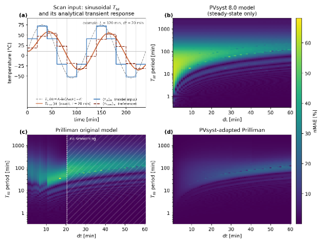
Figure 2.
Example of fit for the roof installation in the no-wind case, U = 21.72 W/m2/K.
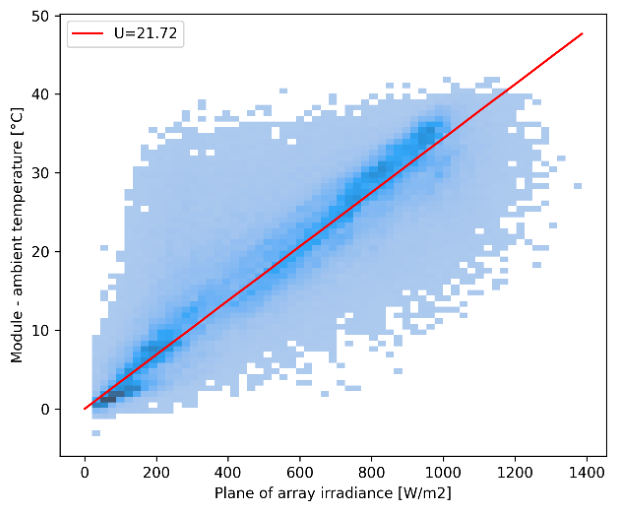
Figure 3.
Error on module temperature models for the rooftop installation. Models show a slight temperature overestimation.
Figure 3.
Error on module temperature models for the rooftop installation. Models show a slight temperature overestimation.
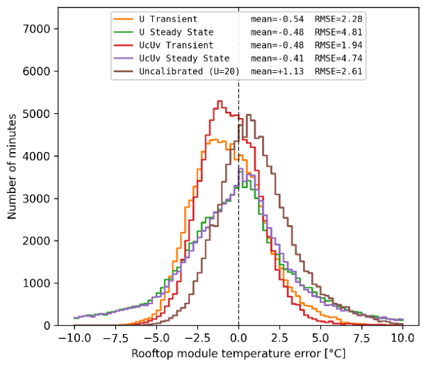
Figure 4.
Error on module temperature models for the ground installation.
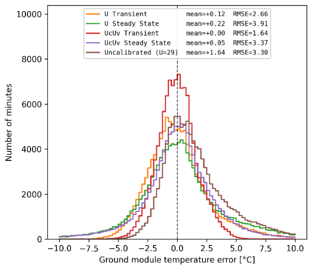
Figure 5.
Roof installation: error on predicted DC yields between simulations, normalised to nominal power.
Figure 5.
Roof installation: error on predicted DC yields between simulations, normalised to nominal power.
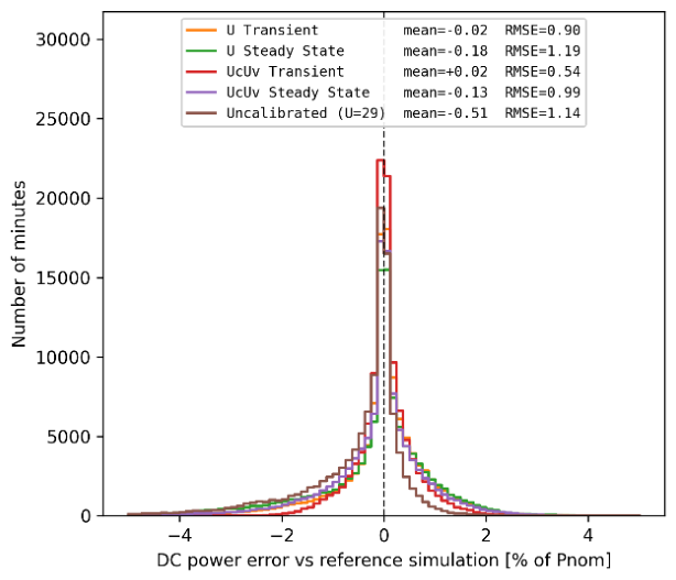
Figure 6.
Roof installation: error between measured DC yields and simulated yields.
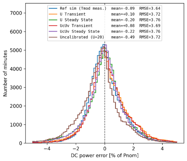

Table 1.
Heat transfer coefficient values for the studied NIST PV arrays.
| Ground | Roof | |
| (=0) | 32.16 [W/m2/K] | 21.72[W/m2/K] |
| 26.42 [W/m2/K] | 19.77 [W/m2/K] | |
| 2.89 [Ws/m3/K] | 1.23 [Ws/m3/K] | |
| Default | 29 [W/m2/K] | 20 [W/m2/K] |
Table 2.
Error on modelled temperature for steady-state and transient models in all scenarios.
| Model | Ground | Roof | ||
|---|---|---|---|---|
| MBE [°C] | RMSE [°C] | MBE [°C] | RMSE [°C] | |
| U transient | 0.12 | 2.66 | -0.54 | 2.28 |
| U steady state | 0.22 | 3.91 | -0.48 | 4.81 |
| UcUv transient | 0.00 | 1.64 | -0.48 | 1.94 |
| UcUv steady state | 0.05 | 3.37 | -0.41 | 4.74 |
| Default transient | 1.64 | 3.30 | 1.13 | 2.61 |
Table 3.
Expected error on modelled DC yield.
| Model | Ground | Roof | ||
|---|---|---|---|---|
| MBE [%] | RMSE [%] | MBE [%] | RMSE [%] | |
| U transient | -0.02 | 0.90 | 0.18 | 0.77 |
| U steady state | -0.18 | 1.19 | -0.11 | 1.56 |
| UcUv transient | 0.02 | 0.54 | 0.17 | 0.63 |
| UcUv steady state | -0.13 | 0.99 | -0.13 | 1.55 |
| Default transient | -0.51 | 1.14 | -0.40 | 0.96 |
Table 4.
Error on modelled DC yield compared to measured yield.
| Model | Ground | Roof | ||
|---|---|---|---|---|
| MBE [%] | RMSE [%] | MBE [%] | RMSE [%] | |
| Measured temp. | -1.77 | 4.99 | -0.09 | 3.64 |
| U transient | -1.79 | 5.07 | 0.10 | 3.72 |
| U steady state | -1.95 | 4.89 | -0.20 | 3.76 |
| UcUv transient | -1.75 | 5.04 | 0.08 | 3.69 |
| UcUv steady state | -1.90 | 4.86 | -0.22 | 3.76 |
| Default transient | -2.28 | 5.14 | -0.49 | 3.72 |
Table 5.
Effect of the simulation time step on the transient model, using the wind measurement.
| dt [min] | TArray vs meas. | DC power vs ref. sim. | ||
|---|---|---|---|---|
| MBE [°C] | RMSE [°C] | MBE [%] | RMSE [%] | |
| 1 | -0.48 | 1.94 | 0.17 | 0.63 |
| 2 | -0.51 | 1.96 | 0.19 | 0.64 |
| 5 | -0.55 | 2.00 | 0.21 | 0.66 |
| 10 | -0.58 | 2.01 | 0.21 | 0.66 |
| 15 | -0.59 | 2.01 | 0.21 | 0.65 |
Disclaimer/Publisher’s Note: The statements, opinions and data contained in all publications are solely those of the individual author(s) and contributor(s) and not of MDPI and/or the editor(s). MDPI and/or the editor(s) disclaim responsibility for any injury to people or property resulting from any ideas, methods, instructions or products referred to in the content. |
© 2026 by the authors. Licensee MDPI, Basel, Switzerland. This article is an open access article distributed under the terms and conditions of the Creative Commons Attribution (CC BY) license (http://creativecommons.org/licenses/by/4.0/).
Copyright: This open access article is published under a Creative Commons CC BY 4.0 license, which permit the free download, distribution, and reuse, provided that the author and preprint are cited in any reuse.