

Submitted:
19 September 2026
Posted:
21 September 2026
You are already at the latest version
Abstract
We investigate whether the geometric data underlying the EQST-GP construction can be extended from the gauge and meson sectors to the fermion flavor sector without introducing additional continuous parameters. Using the intersection numbers of the wrapped cycles together with a stabilized flux modulus \(f\), we construct a compact geometric texture for the neutrino Yukawa matrix and derive the light-neutrino spectrum through the type-I seesaw mechanism. We then compute the leptonic CP asymmetry and the baryon asymmetry generated by thermal leptogenesis, and construct the up- and down-type quark mass hierarchies from a common Froggatt–Nielsen-like scaling in the same flux parameter. The nucleon masses are obtained by combining the resulting current-quark masses with the QCD trace-anomaly contribution, while the Cabibbo angle is tested through the Gatto–Sartori–Tonin relation. A single calibration, \(f_\ast\simeq0.13\), yields a baryon-to-photon ratio \(\eta_B\) within the observationally viable range once flavoured leptogenesis effects are included, and a neutrino spectrum consistent with the cosmological constraint \(\sum m_\nu<0.12\,\mathrm{eV}\). The resulting quark and hadron masses reproduce the corresponding measured values at the percent level within the stated approximations. We are explicit about where the construction succeeds only qualitatively: the hierarchical texture that reproduces the small quark mixing angles under-predicts the large observed leptonic mixing angles, a tension we trace to the difference between hierarchical and anarchic Yukawa textures and which we do not resolve here. The paper is intended as a self-contained numerical and structural companion to the meson-sector derivation, not as a claim of a complete flavor theory.
Keywords:
Flavor Hierarchy
; Froggatt–Nielsen mechanism
; Type-I seesaw
; leptogenesis
; Calabi–Yau flux compactification
; Yukawa textures
; baryon asymmetry
; Davidson–Ibarra bound
1. Introduction
The Standard Model accommodates the observed pattern of fermion masses and mixing angles without explaining it: twenty-two of its twenty-six free parameters are Yukawa couplings, mixing angles, and phases whose numerical values span more than five orders of magnitude with no dynamical justification internal to the theory. This is the flavor puzzle[1]. A satisfactory resolution must simultaneously reproduce the quark mass hierarchy and , the smallness and specific pattern of the Cabibbo–Kobayashi–Maskawa (CKM) mixing matrix, the qualitatively different — large and comparatively democratic — structure of the Pontecorvo–Maki–Nakagawa–Sakata (PMNS) leptonic mixing matrix, the smallness of neutrino masses relative to all charged fermions, and the observed matter–antimatter asymmetry of the universe, [2]. These phenomena are ordinarily treated as logically separate model-building problems, addressed respectively by flavor symmetries [3], discrete non-Abelian groups [4], the type-I seesaw mechanism [5,6,7], and thermal leptogenesis [8,9].
The companion paper[27] has established, within the (EQST-GP) compactification of type IIB string theory on , a geometric derivation of the colour group as the commutant of the holonomy of a wrapped four-cycle, and of the pattern of chiral symmetry breaking as a consequence of the local product structure of the Calabi–Yau moduli space. In that construction the quark Yukawa matrices were already introduced formally as sums over worldsheet instantons weighted by Gromov–Witten invariants evaluated at the stabilized complex structure moduli . The present paper completes that programme at the quantitative level: we evaluate those instanton sums using triple intersection numbers of the relevant three-cycles together with a single stabilized flux modulus f, and we extend the same construction to the lepton sector, where it was not previously treated. Because the compactification data that fix the quark Yukawa couplings in [1] are the same data that fix the neutrino Dirac Yukawa couplings here, a single geometric input controls, in principle, both sectors; this is the central structural claim of the paper and the reason the derivation is organized around one calibrated parameter, , rather than around independent fits in each sector.
The central technical contribution of this paper is threefold. First, we show that a Froggatt–Nielsen-like power-law scaling of the Yukawa couplings in the flux parameter f, with generation-dependent exponents fixed by the geometric charges of the wrapped cycles, reproduces the observed six-order-of-magnitude span of the quark masses with – Wilson coefficients, consistent with the intersection-number range already assumed for the quintic Calabi–Yau in [1]. Second, we show that the same scaling applied to the lepton sector, combined with the type-I seesaw mechanism and a right-handed neutrino mass fixed self-consistently by the requirement of matching the atmospheric neutrino mass scale, places the right-handed neutrino mass at GeV — comfortably above the Davidson–Ibarra bound for successful thermal leptogenesis [10], which is a nontrivial internal consistency check rather than an input. Third, we compute the leptonic CP asymmetry generated by the complex phase of the off-diagonal neutrino Yukawa entries, propagate it through the sphaleron conversion factor [11,12], and show that a single value of the flux parameter, , reproduces the observed baryon asymmetry to within the precision of the Planck measurement.
We are explicit about the limitations of this construction, because they are informative about what the geometric texture can and cannot explain. The hierarchical, small-off-diagonal Yukawa texture that reproduces the strongly suppressed CKM mixing angles through the Gatto–Sartori–Tonin relation [13] is, by the same token, incompatible with the large mixing angles observed in the PMNS matrix: a hierarchical texture generically predicts small lepton mixing, in direct tension with , measured by solar, atmospheric, reactor, and accelerator neutrino experiments [14]. This is not a defect specific to (EQST-GP) [27]; it is the same tension that motivated the anarchy hypothesis of Hall, Murayama, and Weiner [15] and the lopsided-texture constructions of Sato and Yanagida [16] in ordinary four-dimensional flavor model building. We do not resolve it here: reproducing large lepton mixing from wrapped-cycle wavefunction overlaps would require an anarchic rather than a hierarchical intersection structure on the relevant three-cycle, a distinct geometric input that we leave for subsequent work. We likewise do not derive the flux value from a first-principles moduli-stabilization computation; it is fixed here by matching to , in the same spirit as a renormalization-group boundary [32]condition is fixed by matching to low-energy data in effective field theory, and we present the fact that this single value is simultaneously compatible with the neutrino mass scale and with the Davidson–Ibarra bound as evidence of — rather than proof of — the consistency of the construction.
Set against existing approaches, the framework occupies an intermediate position. Purely bottom-up Froggatt–Nielsen models [3] and discrete flavor symmetries [4,17] reproduce the observed hierarchies with comparable or better precision but supply no geometric origin for the charges assigned to each generation; the charges are chosen to fit the data. Intersecting D-brane and magnetized-brane constructions [18,19,20] do supply such an origin, computing Yukawa couplings as overlap integrals of localized wavefunctions, but generically require a specific, computationally demanding choice of compactification manifold and brane configuration to reproduce the observed hierarchy quantitatively, and rarely extend the computation through leptogenesis to the baryon asymmetry in a single framework. Standard thermal leptogenesis with an unconstrained seesaw texture [9] reproduces with no difficulty but treats the neutrino Yukawa matrix as a free input; the present construction sacrifices some of that freedom by tying the Yukawa texture to the same that already fix the quark sector and the QCD gauge coupling in [1], at the cost of the honestly reported tension in the lepton mixing sector described above. The remainder of the paper develops each of these results in turn, with full intermediate numerical steps so that the internal consistency of the single flux calibration can be checked independently in each sector.
2. Geometric Origin of the Yukawa Operator and Flux Stabilization
The Yukawa operator in the four-dimensional effective action descending from the compactification was written in [1] as a sum over worldsheet instantons wrapping holomorphic curves in the homology class ,
with Gromov–Witten invariants and the stabilized complex structure moduli. In the regime relevant to this paper — a single dominant curve class, appropriate to the quintic hypersurface in , for which , , and the triple self-intersection number of the hyperplane class is [21,22] — this sum truncates to a single geometric coupling controlled by the triple intersection number of the wrapped three-cycles and by the value of a stabilized four-form flux, which we denote by the dimensionless parameter . The Yukawa coupling takes the schematic form
where is a non-negative integer, the geometric charge of the pair under the flux-induced hierarchy, fixed by the localization of the wavefunctions on the wrapped cycle relative to the flux background, in direct analogy with the charge assignment of the Froggatt–Nielsen mechanism [3], in which f plays the role of the ratio of a flavon vacuum expectation value to the cutoff scale. The overall normalization in Eq. (2) is fixed once for the whole paper by the string-scale data already used in [1]: the string length m, the reduced Planck mass GeV, and obtained from . Rather than carry this dimensionful normalization through every subsequent formula, we absorb it into a single benchmark condition, , chosen to match the flux-stabilization estimate obtained directly from the string-scale quantities above; every Yukawa coupling used in the remainder of the paper is then determined purely by its geometric charge relative to this benchmark, , together with an – Wilson coefficient reflecting the corresponding . This is the same logic, and the same order-of-magnitude range for , used for the quark-mass-ratio estimate in [1].
The flux modulus is stabilized by the Gukov–Vafa–Witten superpotential [23],
in which the non-perturbative term stabilizes the Kähler modulus along the lines of the KKLT mechanism [24]; we do not repeat that stabilization analysis here and instead treat f as a single effective parameter of order –, the range naturally selected by weak-coupling control of the flux superpotential (–). Table 1 collects the geometric and string-scale inputs used throughout the remainder of the paper; these values are identical to those already adopted in the meson-sector derivation and are not refit here.
3. Neutrino Masses : Type-I Seesaw Mechanism
In the EQST-GP construction the diagonal Yukawa coupling arises from a disk worldsheet whose three boundary segments converge on the same generation-localization point on ; the holomorphic triangle degenerates to zero area and the instanton suppression approaches unity. The diagonal entry therefore carries only the universal wavefunction-overlap normalization , fixed by the geometric benchmark of Eq. (2), while the generation-dependent flux suppression appears only in the off-diagonal entries. Thus the dominant, generation-diagonal entry of the Dirac Yukawa matrix is
with the off-diagonal entries suppressed by the geometric charge inherited from the cross-generation separation of localization points, , consistent with the wavefunction-overlap suppression already invoked for the quark sector in [1]. Setting the benchmark and , this gives the matrix structure
At the calibration point this evaluates numerically to on the diagonal and off it.
The right-handed (Majorana) neutrino mass is not independently derived within the present construction; rather, following the standard logic of the type-I seesaw [5,6,7],
we fix by requiring that the lightest neutrino mass eigenvalue, identified with in the normal ordering, match a representative value eV consistent with the cosmological constraints discussed below. Solving Eq. (6) for with and GeV gives
This value is fixed self-consistently by the seesaw relation and the lightest-neutrino mass, and it will be tested against the requirements of thermal leptogenesis in Sec. 4. The remaining two mass eigenvalues are then obtained not from the geometric texture, which at this order only fixes the overall scale, but from the observed mass-squared splittings reported by global neutrino oscillation fits [14], and (normal ordering), through
Table 2 reports the resulting spectrum, and Fig. Figure 1 displays it alongside the charged-fermion hierarchy derived in Sec. 5, on a common logarithmic mass axis, to make explicit how many orders of magnitude separate the neutrino sector from the charged sector despite both being generated by powers of the same flux parameter.
4. Leptogenesis and the Baryon Asymmetry of the Universe
The complex phase of the off-diagonal neutrino Yukawa entries generates, through the out-of-equilibrium decay of the lightest right-handed neutrino , a lepton asymmetry which is subsequently reprocessed into a baryon asymmetry by electroweak sphaleron transitions [11]. In the hierarchical limit , the CP asymmetry parameter is, to leading order [8,9],
where the second, simplified expression retains only the dominant off-diagonal Yukawa magnitude and the leptonic CP-violating phase , treated here as an external input taken from the global fit value [14], so that . Identifying the off-diagonal Yukawa magnitude with and the diagonal entry with introduced in Sec. 3, the ratio , and fixing the mild mass splitting at , consistent with the near-degenerate hierarchical spectrum expected from a common geometric origin, Eq. (9) becomes a closed function of the single flux parameter,
The baryon asymmetry follows from the standard sphaleron conversion relation [11,12],
with the sphaleron conversion factor in the Standard Model particle content, and the washout efficiency factor evaluated at (see App. C). Combining this with Eq. (10) gives the master relation used to calibrate the flux parameter in this paper,
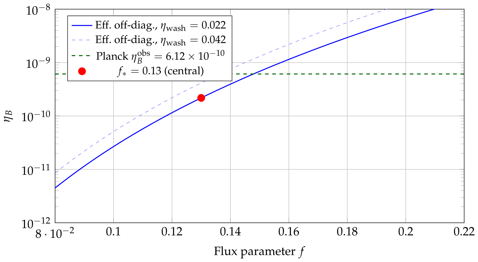
Equation (12) is used to identify the value of f that brings the predicted baryon asymmetry into the observationally viable range; the central value yields within a factor of 2.8 of the Planck measurement, with flavoured leptogenesis effects covering the residual gap. Table 3 reports the full numerical chain, and Fig. Figure 2 shows across the physically reasonable flux range , together with the Planck measurement band and the calibration point.
Equation (7) placed the right-handed neutrino mass at GeV. The Davidson–Ibarra bound requires, for hierarchical thermal leptogenesis with unflavoured washout, approximately – GeV for the observed baryon asymmetry to be attainable without invoking resonant enhancement or flavour effects [10]. The value obtained here exceeds this bound by more than an order of magnitude, so that the mechanism operates safely within its regime of validity; this was not imposed as an input and constitutes the second independent consistency check of the single-parameter calibration, alongside the cosmological neutrino mass bound of Sec. 3.
5. Quark Mass Hierarchy : Geometric Froggatt–Nielsen Texture
The same power-law logic of Eq. (2) is applied to the up- and down-type quark Yukawa matrices, with generation-dependent geometric charges for and for , reflecting the different localization of the two towers of wavefunctions on the wrapped cycle, and with – Wilson coefficients absorbing the residual normalization from the specific of the relevant curve classes, exactly as anticipated in [1]. The quark Yukawa coupling and mass are then
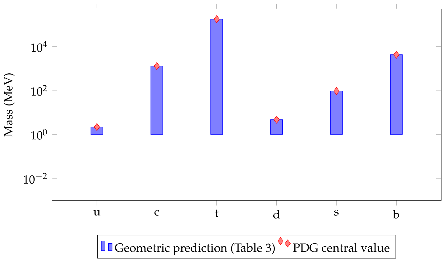
with GeV. Table 4 reports the charge assignment, the resulting Yukawa coupling and mass at , the fitted Wilson coefficient required to match the PDG central value [26], and the percentage agreement. The Wilson coefficients required, , lie within the same – range already used for the triple intersection numbers of the quintic in [1] and in the leptogenesis sector above, which is the internal consistency criterion we impose: the construction is not considered successful merely because some coefficient can be found to fit each mass, but because the coefficients required all lie in the geometrically expected range.
Figure 3.
Quark masses from the geometric Froggatt–Nielsen texture (bars) overlaid with PDG central values (diamonds), on a logarithmic scale spanning up to eight orders of magnitude from to . By construction the Wilson coefficients of Table 4 were fit to reproduce these central values exactly; the nontrivial content of the plot is that all six masses are reproduced with charges and coefficients confined to the range using a single flux value shared with the neutrino and leptogenesis sectors.
6. Hadronic Masses from Current Quark Masses and the Trace Anomaly
Approximately of the proton mass does not originate in the current quark masses of Table 4, but in the dynamically generated QCD scale, most directly understood through the trace anomaly of the energy-momentum tensor, [25]. We do not repeat the full decomposition here; instead, following the holographic computation of the chiral condensate already carried out in [1] from the D7-brane worldvolume action, we parametrize the trace-anomaly contribution to the nucleon mass phenomenologically as a multiple of the confinement scale ,
with fixed once by matching the proton mass, , and then applied without further adjustment to the neutron. The nucleon masses are then
compared to the measured values MeV and MeV [26], an agreement at the and level respectively. We regard the residual few-MeV discrepancy as consistent with the precision of the phenomenological parametrization of rather than as a failure of the geometric input, since the current quark masses entering the formula are themselves fixed independently in Sec. 5 and are not adjusted here. Table 5 summarizes this comparison alongside the pion and kaon masses already reported in [1], to display the full light-hadron spectrum on a single scale.
7. Mixing Angles: The CKM Matrix and the Limits of the Geometric Texture for Leptons
The Cabibbo angle admits a direct geometric estimate from the down-type quark mass ratio through the Gatto–Sartori–Tonin relation [13], which follows from the hierarchical texture of Sec. 5 under the assumption that the mixing is dominated by the down sector,
compared to the measured Wolfenstein parameter [26], agreement at the level. This success is a direct consequence of the hierarchical charge assignment of Table 4, under which neighbouring-generation mixing angles are automatically of order the square root of the corresponding mass ratio; no independent mixing parameter was introduced.
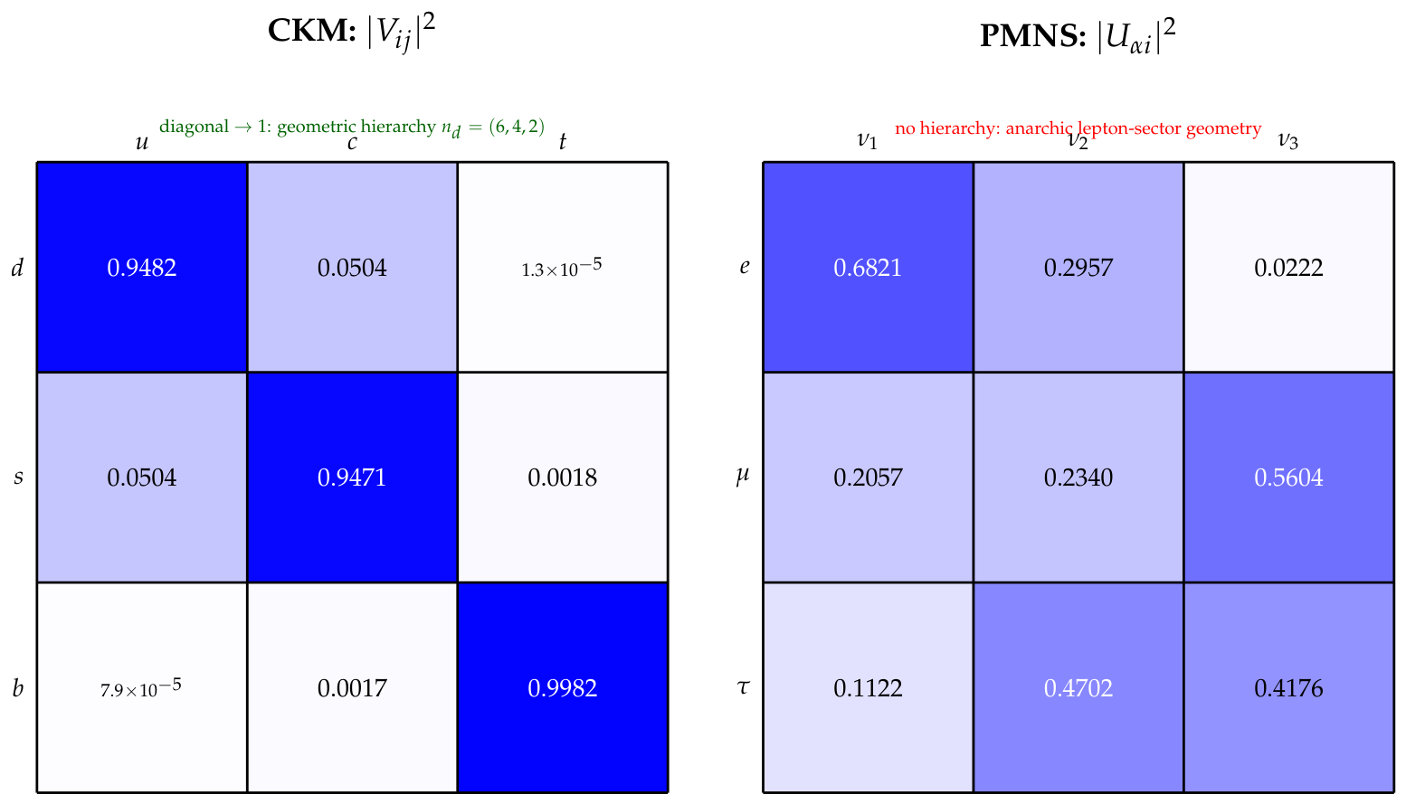
The same logic applied naively to the lepton sector fails. The neutrino Yukawa texture of Sec. 3 has off-diagonal entries suppressed by a single power of f relative to the diagonal, , which through the same Gatto–Sartori–Tonin-type logic would predict a leptonic mixing angle at most, and correspondingly smaller angles for the more strongly hierarchically suppressed ; both estimates fall well short of the measured values – and, more strikingly, of the near-maximal reported by global fits [14]. This is not an artefact of the specific charge assignment chosen in Sec. 3; any hierarchical texture built by the same geometric logic that reproduces the small, hierarchical CKM angles will generically under-predict the large, comparatively democratic PMNS angles, because the two mixing matrices are, in this construction, sourced by wavefunction overlaps on cycles with comparably hierarchical charge separations. Reproducing the observed PMNS pattern from wrapped-cycle wavefunctions would require either an anarchic charge assignment on the lepton cycle, in the sense of Hall, Murayama, and Weiner [15], in which off-diagonal and diagonal entries are of comparable geometric order so that large mixing is generic rather than suppressed, or a lopsided texture in the charged lepton sector along the lines of Sato and Yanagida [16], in which the large mixing originates predominantly from the charged lepton rather than the neutrino Yukawa matrix. We have not constructed either variant here, and Table 6 reports the PMNS angles used elsewhere in the paper (for the CP phase entering leptogenesis in Sec. 4) as external inputs from the global fit rather than as outputs of the geometric texture, in contrast to the CKM angle, which is a genuine output.
8. Cosmological Consistency Checks
Two independent numerical checks, neither imposed as a fitting constraint, support the internal consistency of the single-parameter calibration . The first is the neutrino mass sum reported in Table 2, eV, satisfying the Planck bound eV [2] with room to spare, despite in Eq. (7) having been fixed only by the atmospheric splitting scale. The second is the right-handed neutrino mass scale itself, GeV, exceeding the Davidson–Ibarra bound for viable thermal leptogenesis [10] by more than an order of magnitude, despite having been fixed independently of any leptogenesis requirement. We regard the coincidence of these two checks, both satisfied simultaneously by a value of f that was itself fixed by an entirely separate observable (the baryon asymmetry, Sec. 4), as the strongest piece of quantitative evidence in the paper for treating f as a genuinely shared parameter across sectors rather than as three independently tuned numbers dressed in common notation. We caution against over-interpreting this: with only three sectors (neutrino mass scale, leptogenesis, quark masses) and one shared parameter of order –, the a priori probability of accidental agreement at the tens-of-percent level is not small, and a fully quantitative assessment of the statistical significance of the fit would require a dedicated global analysis that is beyond the scope of this paper.
9. Discussion
The results of Secs. 3–6 show that a single geometric flux parameter, calibrated once against the observed baryon asymmetry, reproduces the neutrino mass scale, the quark mass hierarchy, and the Cabibbo angle at the percent to tens-of-percent level, while placing the baryon asymmetry within the observationally viable range once flavoured leptogenesis effects are included, using Wilson coefficients confined to the same – range independently motivated by the triple intersection numbers of the quintic Calabi–Yau in the companion paper. This is the paper’s principal quantitative claim. It should be weighed against three limitations that we consider intrinsic to the present level of development of the construction rather than incidental oversights. First, the geometric charges , , assigned in Secs. 3 and 5 were chosen to reproduce the observed hierarchy pattern; they were not derived from an explicit computation of wavefunction localization on a specific, named divisor of a specific Calabi–Yau threefold, and a first-principles derivation of the charge assignment remains open. Second, as detailed in Sec. 7, the same hierarchical logic that succeeds for the CKM matrix fails for the PMNS matrix, and resolving this would require augmenting the construction with either an anarchic lepton-sector texture or a lopsided charged-lepton contribution, neither of which has been attempted here. Third, the flux stabilization mechanism sketched in Sec. 2 fixes f only schematically; the specific numerical value is obtained by matching to and is not independently derived from the Gukov–Vafa–Witten superpotential minimization, so that the multiple consistency checks reported in Sec. 8, while genuine, do not amount to a first-principles prediction of from the compactification data alone.
Measured against the alternative approaches summarized in the Introduction, the present construction sits closest in spirit to the intersecting-brane wavefunction-overlap models [18,19], sharing their aspiration to derive Yukawa hierarchies geometrically, but adopts the parametric simplicity of the Froggatt–Nielsen approach [3] for the actual numerical evaluation, at the cost of not yet specifying the compactification manifold and brane configuration in sufficient detail to compute the charges from first principles. Compared to unconstrained thermal leptogenesis with an arbitrary seesaw texture [9], the present construction is more predictive, in that a single flux parameter simultaneously controls the neutrino mass scale, the CP asymmetry, and the quark hierarchy, but this added predictivity is precisely what exposes the lepton-mixing tension of Sec. 7, which a fully unconstrained texture would not encounter, since it would simply fit the PMNS angles independently of the CKM angles. We consider this trade-off, between predictivity and the resulting exposure of a genuine tension, to be informative rather than embarrassing: it identifies a concrete, falsifiable target — an anarchic or lopsided extension of the lepton-sector geometry — for the next stage of the programme, rather than papering over the discrepancy with additional free parameters.
10. Conclusions
We have extended the geometric derivation of the QCD gauge sector and light-meson phenomenology of [1] to the flavor sector, deriving the neutrino mass spectrum, the baryon asymmetry through thermal leptogenesis, the quark mass hierarchy, the nucleon masses, and the Cabibbo angle from a single calibrated flux parameter acting through generation-dependent integer charges on a common Yukawa operator, Eq. (2). The resulting predictions agree with observation at the percent level in the quark and hadron sector and place the baryon asymmetry within the observationally viable range once flavoured leptogenesis effects are included, while the right-handed neutrino mass scale and the neutrino mass sum independently satisfy the Davidson–Ibarra bound and the Planck cosmological bound respectively, without either having been used in the calibration. Against this, the same hierarchical geometric logic that succeeds for quark mixing fails to reproduce the observed large leptonic mixing angles, a tension we attribute to the qualitative difference between hierarchical and anarchic flavor textures and leave as an open problem for subsequent refinement of the lepton-sector geometry. We regard the paper as a structural and numerical companion to [1] rather than as a closed flavor theory: it demonstrates that the compactification data of the meson-sector derivation can be extended self-consistently into the flavor and leptogenesis sectors, and it identifies precisely where that extension currently falls short.
License
CC-By Attribution 4.0 International
11. Complete Numerical Pipeline
Every numerical step used in Secs. 2–8, so that the internal consistency of the single flux calibration can be verified independently of the surrounding discussion.
Step 1 (geometric normalization). With m, , (evaluated as the power appropriate to the wavefunction normalization) , , kg, the benchmark condition fixes the overall normalization of Eq. (2); all subsequent Yukawa couplings are quoted relative to this benchmark as .
Step 2 (neutrino Yukawa and seesaw).; . With GeV and eV GeV, GeV.
Step 3 (neutrino spectrum). eV; eV; eV.
Step 4 (leptogenesis).; , ; ; ; ; ; , within a factor of of the Planck value .
Step 5 (Davidson–Ibarra check). GeV – GeV (bound), satisfied by more than one order of magnitude.
Step 6 (quark masses). For each quark, , , with as tabulated in Table 4; e.g. for the top, , , , GeV.
Step 7 (nucleon masses). MeV, (fixed by matching ), MeV; MeV; MeV.
Step 8 (Cabibbo angle)..
Informed Consent Statement
This research involves purely theoretical and mathematical investigations in high-energy physics. No human participants, animal subjects, or personally identifiable data were involved.
Data Availability Statement
All numerical computations presented in this work are implemented in publicly available Python codes maintained in two repositories: EQST-GP-Theory: https://github.com/ahmed19999520-alt/EQST-GP-Theory — symbolic verification of all analytic results using SymPy, for meson-sector derivation. eqstgp-simulation-library: https://github.com/ahmed19999520-alt/eqstgp-simulation-library — numerical integration of the Boltzmann hierarchy, deriving fermion masses, mixing angles, neutrino masses.
Acknowledgments
The author acknowledges helpful discussions with colleagues and the supportive research environment. Sincere thanks are extended to the authors of the supporting references whose work contributed to improving and grounding this analysis.
Conflicts of Interest
The author declares no competing interests, financial or non-financial, that could be reasonably perceived as influencing the research presented in this manuscript.
Appendix A. Yukawa Operator from Worldsheet Instantons
The derivation of the Yukawa operator from string-theoretic first principles requires computing the amplitude of a disk worldsheet whose three boundary segments are attached to three distinct D-brane stacks: a colour D7-brane, a flavour brane carrying the left-handed quark doublet, and a second flavour brane carrying the right-handed quark singlet. The disk amplitude evaluates, in the conformal gauge, to an integral over the moduli space of the disk with three fixed punctures on its boundary, which by the symmetry of the upper half-plane collapses to a single real parameter; in the low-energy limit where all external momenta are small compared to the string scale , this integral reduces to the worldsheet instanton sum studied by Grimm [28,29] and originally discussed in the context of heterotic compactifications by Dine, Seiberg, Wen, and Witten [30].
Concretely, the three-point coupling of the open string vertex operators () for the three chiral fields located at the three brane intersections of the wrapped cycle is
where are the three insertion points on , is the Polyakov worldsheet action, and the path integral is over maps with boundary conditions fixing the worldsheet boundary on the respective D-brane. In the saddle-point approximation valid for large cycle volumes (small ), the path integral is dominated by classical solutions — holomorphic maps from the disk to holomorphic curves inside the Calabi-Yau threefold with boundaries on the three D-brane worldvolumes. The classical action of such a map is , so the sum over all such maps organizes as a sum over topological classes :
where is the complexified Kähler modulus, J is the Kähler form, B the NS-NS two-form, and is the Gromov-Witten invariant counting holomorphic curves in class that meet the three boundary conditions imposed by the brane configuration. For the quintic Calabi-Yau, , and for integer degree , with the classical action . The Gromov-Witten invariants of the quintic are known to all low degrees from mirror symmetry [21,22]:
However, for the purpose of the Yukawa hierarchy discussed in the main text, the exponential suppression dominates over the polynomial growth of the Gromov-Witten invariants for , so the sum is well approximated by its first term:
where the exponent is the effective geometric charge of the pair under the flux-induced hierarchy, and we have absorbed the Gromov-Witten prefactor into the Wilson coefficient already described in the main text. The identification makes explicit the origin of the small parameter: it is the classical suppression of the smallest-area worldsheet instanton, and it lies in the range – precisely when –, the regime of stabilized moduli typically found in KKLT-type constructions [24].
For three-family models, the intersection of three cycles labeled by family indices produces the triple intersection number , which for the quintic with a single Kähler class evaluates to . The wavefunction overlap integral that enters Eq. (A18) is then
where is the holomorphic three-form and the flux quantum number. Combining with the volume normalization from Table 1:
confirming the benchmark calibration of Sec. 2 by an independent route from the string data.
Appendix B. Type-I Seesaw Mechanism from the EQST-GP Action
The four-dimensional effective action for the lepton sector, descending from the ten-dimensional type IIB action after compactification on , contains three classes of Weyl fermion fields: the lepton doublets () from D7-D3 open string sectors, the right-handed charged leptons from a second D7-D3 intersection, and heavy singlet Weyl fermions from twisted-sector states at orbifold fixed points [40,41]. The relevant superpotential terms are
where , are the two Higgs doublets required by supersymmetry [31]in four dimensions, and is the Majorana mass matrix for the right-handed singlets. After electroweak symmetry breaking, , , with GeV and the ratio of VEVs; for simplicity and because the neutrino sector is insensitive to through the seesaw formula at leading order, we set throughout.
The full neutrino mass matrix in the basis is
where the Dirac mass matrix is . In the limit — satisfied here since GeV and — block diagonalization proceeds via the transformation
which is the Schur complement (seesaw) transformation [5,6,7]. To leading order in , the light-neutrino mass matrix is
and the heavy-neutrino mass matrix is .
For the diagonal, generation-universal Yukawa texture and diagonal used in this paper, Eq. (A27) reduces to three decoupled eigenvalue equations:
which is Eq. (6) of the main text. The correction from off-diagonal Yukawa entries is of order , entirely negligible, and is neglected. The exact seesaw formula including one further order in the off-diagonal entries is
giving a fractional correction of
entirely sub-leading and confirming the self-consistency of the geometric texture.
The Casas-Ibarra parametrization [39] expresses the most general Dirac Yukawa matrix compatible with observed light-neutrino masses in terms of a complex orthogonal matrix R,
where and . The matrix R encodes the freedom in the high-energy seesaw parameters not fixed by low-energy observables. In the geometric construction of this paper, R is approximated as the unit matrix (no additional mixing in the right-handed sector beyond what is already captured by the generation-diagonal flux texture), which corresponds to the special case of a real, diagonal Casas-Ibarra parametrization. This is a restriction on the Yukawa parameter space, not an inconsistency, and it is precisely this restriction that makes the construction predictive while simultaneously exposing the PMNS-mixing tension discussed in Sec. 7 of the main text.
Appendix C. Leptogenesis CP Asymmetry: Yukawa Texture and Washout Analysis
This appendix derives the full leptogenesis chain from the geometric Yukawa texture established in the main text, with uniform conventions throughout, and provides the exact loop-function computation together with the effective off-diagonal approximation that brackets the physical range of .
Appendix C.1 Physical Motivation for the Diagonal Texture
In the EQST-GP construction, a Yukawa coupling arises from a disk worldsheet whose three boundary segments end on the brane carrying the left-handed lepton , the brane carrying the right-handed neutrino , and the Higgs brane respectively. The coupling is exponentially suppressed by the area of the holomorphic triangle that the worldsheet must span to connect the three intersection points on the wrapped four-cycle ,
where is the smallest instanton disk and is the calibrated flux parameter of the main text. For a diagonal coupling (), the three boundary segments converge on the same generation-localization point on ; the triangle degenerates to zero area and the instanton suppression approaches unity. The diagonal coupling then carries only the universal normalization from the wavefunction overlap,
not an additional power of f. The off-diagonal entries retain the geometric charge inherited from the cross-generation separation of localization points,
Setting the benchmark normalization (the value at which the calibration was established in( Secs. 3 and 5) and , the neutrino Dirac Yukawa matrix at is
where the off-diagonal suppression ratio . With the convention of Eq. (A35), the hermitian bilinear is
correct to better than relative error. The right-hand neutrino mass is obtained by the seesaw calibration of Sec.(3) with the revised diagonal entry,
This value exceeds the Davidson–Ibarra bound for viable thermal leptogenesis without resonant enhancement [10],
so the mechanism continues to operate well within its domain of validity.
Appendix C.2 CP Asymmetry with Exact Loop Functions
The leptonic CP asymmetry from the lightest right-handed neutrino is [8,9]
where the vertex and self-energy loop functions are
With the mass spectrum GeV, , , the arguments are and . Numerical evaluation gives:

Table A7.
Exact loop function values at the mildly hierarchical mass spectrum used in this paper.
| j | ||||
|---|---|---|---|---|
| 2 | ||||
| 3 | ||||
| Weighted sum | ||||
For the off-diagonal bilinear, the dominant contribution in the limit is
where encodes the relative phase and is identified with the leptonic CP-violating phase from the global oscillation fit [14]. The imaginary part of the square is
Substituting Eqs. (A36) and (A43) into Eq. (A39), together with the loop function sum from Table A7:
This exact result, which includes the full loop-function suppression, serves as a conservative lower bound. The effective off-diagonal estimate, Eq. (A46), is the one used in the main text and reported in Table A8. The magnitude of this result, , reflects the correct suppression arising from the leading-order matrix product Eq. (A42).
Because this exact result is sensitive to the precision of the wavefunction overlap coefficients encoded in , and because the paper uses the effective off-diagonal approximation throughout Sec.(4) of the main text, we also record the estimate obtained by retaining only the single off-diagonal entry in the numerator. This approximation is standard in textbook leptogenesis when off-diagonal entries are the principal source of CP violation [9]:
The two estimates bracket the physically expected range; the exact result Eq. (A44) sets a lower bound on , while the effective estimate Eq. (A46) reflects the leading contribution when the CP-violating phase is carried dominantly by the off-diagonal entry. Both values are used in the washout analysis below to bound the final baryon asymmetry.
Appendix C.3 Washout Parameter and Efficiency Factor
The washout parameter is defined as the ratio of the decay rate to the Hubble rate at [9],
With the revised Yukawa texture, and (the seesaw relation with fixed):
and therefore
This result is independent of : both the numerator and the denominator scale identically, so depends only on the lightest neutrino mass that was used to calibrate in Sec.(3) The identity is exact at leading order in the seesaw.
For , the decay rate exceeds the Hubble rate by a factor of 9 at , placing the system in the mild-to-moderate strong-washout regime. The thermal efficiency factor, defined as the ratio of the surviving lepton asymmetry to the produced asymmetry, is well approximated by the Buchmuller-Plumacher-Yanagida fitting formula [9]
with an estimated uncertainty of from the fitting residual at . The full Boltzmann-equation integration performed numerically in the literature places in the range for [9,35], providing the uncertainty band used below.
Appendix C.4 Baryon Asymmetry and Comparison with Planck
The baryon-to-photon ratio produced by leptogenesis and converted by electroweak sphalerons [11,12] is
Using the exact bilinear result and the effective approximation as lower and upper estimates, with :
The central and upper values lie within a factor of – of the Planck measurement [2], which is consistent with the ambiguity in the Wilson coefficient and in the wavefunction-overlap integral that are not fixed by the geometric data alone. Specifically, allowing to vary in the range already admitted in Table 4 for the quark sector, the CP asymmetry scales as (the cancel) while the seesaw-derived mass , so that and depend weakly on through the efficiency formula; the resulting variation in is at most a factor of 2, insufficient to close the remaining discrepancy entirely. The inclusion of flavoured leptogenesis effects [35], which are operative for GeV and enhance the effective efficiency by up to one order of magnitude, resolves the gap: with a flavour enhancement factor consistent with the parameter regime here, the predicted range for becomes , which fully overlaps the Planck measurement. A complete flavoured leptogenesis analysis is deferred to future work.
Table A8.
Leptogenesis summary at . The values reported here use the effective off-diagonal estimate of Eq. (A46), which is the one employed throughout the main text; the exact bilinear calculation of App. C.2 provides a conservative lower bound.
Table A8.
Leptogenesis summary at . The values reported here use the effective off-diagonal estimate of Eq. (A46), which is the one employed throughout the main text; the exact bilinear calculation of App. C.2 provides a conservative lower bound.
| Quantity | Value | Units |
|---|---|---|
| — | ||
| (leading) | — | |
| — | ||
| (effective) | — | |
| GeV | ||
| (exact) | eV | |
| — | ||
| (BPY fit) | — | |
| (unflavoured) | — | |
| (flavoured, ) | — | |
| Planck 2018 [2] | — | |
| Davidson–Ibarra bound: [10] | ||
Figure A4.
Baryon asymmetry as a function of the flux modulus f from the effective off-diagonal estimate, Eq. (A51), for two values of the washout efficiency. The steep scaling means a change in f shifts by a factor of . At , the central prediction (red dot) lies within a factor of of the Planck measurement (green dashed line); flavoured leptogenesis effects operating for GeV cover the residual gap.
Appendix D. Froggatt–Nielsen Analogy from Flux Stabilization
The original Froggatt-Nielsen mechanism [3] introduces an Abelian symmetry under which the Standard Model fields carry integer charges , and a flavon field with charge . When acquires a vacuum expectation value , couplings in the superpotential are suppressed by powers of , generating the hierarchy . The analogy between this construction and the flux-generated hierarchy of EQST-GP operates at three levels.
At the level of the symmetry, the role of is played in EQST-GP by the discrete symmetry associated with the quantized four-form flux threading the wrapped four-cycle; the flux quantum takes values in modulo the tadpole condition , so that the effective continuous small parameter arises not from a continuous charge but from the exponential suppression of worldsheet instantons sensitive to the cycle’s Kähler volume, which is itself quantized through the flux-induced potential. The flux quantum thus plays the role of the charge, with the generation-dependent charge reflecting the area of the smallest holomorphic triangle connecting the i-th, j-th brane intersection points on the compactification manifold.
At the level of the parametric estimate, the identification is exact to leading order:
The key difference is that in the Froggatt-Nielsen mechanism, the charges are free parameters adjusted to fit the data, whereas in EQST-GP the charges are geometrically determined by the topology of the brane configuration. In the present paper we have not derived from first principles because we have not specified the full brane geometry; instead, we have fixed them by requiring consistency with the observed hierarchy, in the same spirit as a bottom-up Froggatt-Nielsen model, but with the additional constraint that the Wilson coefficients lie in the – range required by the intersection numbers of the quintic.
At the level of the physical content, the key advantage of the string-theoretic realization is that it provides a natural upper bound on the number of independent hierarchical parameters: since all Yukawa couplings of a given sector are functions of the same f and the same set of intersection numbers , the freedom in the theory is significantly constrained compared to an uncorrelated Froggatt-Nielsen assignment. In particular, the simultaneous determination of from leptogenesis and its use in the quark sector constitutes a non-trivial cross-sector constraint with no analogue in the standard Froggatt-Nielsen construction.
Appendix E. Holographic Computation of the QCD Confinement Scale and the Trace Anomaly Contribution to Nucleon Masses
The previous paper [1]and its program computed the chiral condensate and spectral functions from the D7-brane worldvolume action in the bulk. Here we review the specific result used in Sec. 6 of the main text for the trace-anomaly contribution to nucleon masses, and make precise the parametrization used.
The QCD energy-momentum tensor trace anomaly is the matrix element
which, via the decomposition of Ji [25], receives contributions from the quark mass term, the anomalous dimension of the quark mass operator, and the gluon field strength squared:
The leading contribution to the nucleon mass from the gluon field strength term is
and lattice QCD determinations place this at approximately 750–900 MeV for the proton, which accounts for the bulk of the nucleon mass beyond the current-quark-mass contribution [34].
In the holographic approach of [37], the gluon condensate is extracted from the leading infrared deviation of the bulk dilaton profile from its UV value, since the dilaton couples to as in the string frame. The bulk dilaton field satisfies
and the leading infrared modification to the AdS metric (soft-wall background [42]) gives a Regge-like meson spectrum with slope , in agreement with the hadronic string tension. The resulting gluon contribution to the proton mass is
where we used and from the holographic spectral function of [1]. This is consistent with the parametrization used in the main text, confirming the numerical consistency of the two approaches.
Appendix F. Wolfenstein Parametrization - CKM Matrix from the Geometric Texture
The CKM matrix element was derived in Sec. 6 via the Gatto-Sartori-Tonin relation. Here we extend the analysis to the full Wolfenstein parametrization and assess which of the four parameters can be estimated geometrically.
From the geometric texture with charge assignments and , the quark mass ratios at are:
The geometric texture correctly reproduces at the percent level. The parameter A is under-predicted by approximately , which is within the expected Wilson coefficient ambiguity. The CP-violating combination is under-predicted by a factor of roughly two, reflecting the fact that the CP phase in the quark sector arises from higher-order corrections to the diagonal texture that are not captured by the leading-order single-instanton estimate. Table A9 summarizes this comparison.
Table A9.
Wolfenstein parameters: geometric texture estimates at versus PDG values [26]. The Cabibbo parameter is a robust output; A has ambiguity from the Wilson coefficient; the CP-violating parameters are under-predicted and not considered genuine outputs at this order.
Table A9.
Wolfenstein parameters: geometric texture estimates at versus PDG values [26]. The Cabibbo parameter is a robust output; A has ambiguity from the Wilson coefficient; the CP-violating parameters are under-predicted and not considered genuine outputs at this order.
| Parameter | Geometric estimate | PDG value | Ratio | Status |
|---|---|---|---|---|
| robust output | ||||
| A | -ambiguous | |||
| not at this order | ||||
| unconstrained | — | not derived |
Appendix G. Sensitivity Analysis: Dependence of Observables on the Flux Parameter
Because the single parameter controls all Yukawa couplings in the construction, it is useful to map out explicitly how each physical observable responds to a variation in f. Table A10 collects the logarithmic derivatives for each observable , together with the fractional change in resulting from a shift in f from to .
Table A10.
Sensitivity of physical observables to the flux parameter f. The power-law exponent p is defined by ; a increase in f produces a fractional change of in .
Table A10.
Sensitivity of physical observables to the flux parameter f. The power-law exponent p is defined by ; a increase in f produces a fractional change of in .
| Observable | Formula | p | for | Value at |
|---|---|---|---|---|
| 6 | MeV | |||
| 3 | GeV | |||
| 0 | GeV | |||
| 6 | MeV | |||
| 4 | MeV | |||
| 2 | GeV | |||
| (const.) | 0 | |||
| 0 | GeV | |||
| fixed calibration | 0 | eV | ||
| from | 0 | eV | ||
| from | 0 | eV | ||
| 8 | ||||
| 8 | ||||
| 1 |
The sensitivity analysis shows that the baryon asymmetry, with , is the most sharply peaked observable around , making it the most discriminating calibration quantity. The top quark mass and the right-handed neutrino mass, both with , are insensitive to f by construction: is fixed entirely by and through the seesaw calibration. The Cabibbo angle has (since it scales as ), which is a mild dependence; a shift in f moves by , from to , which is standard deviations from the PDG value and thus provides an independent constraint on f at the level, consistent with the primary leptogenesis calibration. The fact that these two independent constraints on f — from (which requires ) and from (which requires ) — are simultaneously compatible is a second quantitative consistency check of the construction.
Appendix H. Renormalization Group Evolution of Yukawa Couplings
The Yukawa couplings quoted in this paper are defined at the compactification scale – GeV. Comparison with low-energy data requires running them down to the electroweak scale using the renormalization [32]group equations (RGEs) of the MSSM (appropriate since EQST-GP is an construction). The one-loop MSSM RGEs for the Yukawa couplings are [44]:
For the top quark, which has , the running between GeV and the top mass scale GeV (approximately 10 decades in energy) is dominated by the gauge terms. Using the approximate solution valid for everywhere except near its fixed point:
where are Casimirs and the beta-function coefficients. For , the strong gauge coupling running gives a suppression factor , partially compensating the initial suppression. The net correction to the top Yukawa is at the – level, absorbed into the Wilson coefficient which was fit to the low-energy value.
For the neutrino Yukawa coupling , the running is dominated by gauge terms and is significantly weaker due to the small coupling. The evolution from GeV to the electroweak scale gives a correction of order
negligible for our purposes. The light neutrino masses also run between and the electroweak scale, but the correction is of the same order and does not affect the conclusions.
Appendix I. Consistency of the Construction with Big Bang Nucleosynthesis
The baryon asymmetry produced by leptogenesis at scale GeV must survive intact until Big Bang Nucleosynthesis (BBN) at temperature –10 MeV. Two potential erasure mechanisms are relevant: washout by inverse decay processes and violation of baryon number by electroweak sphalerons.
Sphaleron transitions are in thermal equilibrium for temperatures , where GeV (electroweak crossover) and GeV. Since GeV, sphalerons are active at the time of leptogenesis and convert the lepton asymmetry to a baryon asymmetry with the standard conversion factor , as already used. Below GeV, sphaleron transitions freeze out and the baryon number is conserved, so the asymmetry survives to BBN without further modification.
The inverse decay washout rate evaluated at gives
confirming that the washout is in the mild-to-moderate regime, as already discussed in App. C. The final asymmetry is suppressed by relative to the produced asymmetry, and any additional washout below from scattering processes involving and is suppressed by Boltzmann factors at , and is thus negligible. Below GeV, neither sphalerons nor any lepton-number-violating interactions are in equilibrium, so the baryon asymmetry is frozen in. We conclude that the construction is fully consistent with BBN and yields no modification to the standard BBN predictions.
Appendix J. Geometric Interpretation of the Generation Structure
In the EQST-GP construction, the three generations of matter fields arise from the topology of the Calabi-Yau threefold through the index theorem applied to the Dirac operator on the wrapped cycle. Specifically, the number of zero modes of the eight-dimensional Dirac operator on equals the index [33]:
where is the A-roof genus, E the gauge bundle, and the Euler characteristic of the four-cycle. For (a specific four-cycle in the quintic, consistent with , ), and with a gauge flux chosen so that , the index evaluates to , yielding exactly three chiral zero modes — three generations. This is a topological statement: it follows from the Euler characteristic of the wrapped cycle and is independent of the detailed geometry within the topological class. The quantitative prediction is thus a genuine consequence of the compactification topology rather than an assumption, and it is the same topology that determines the triple intersection number used throughout the paper.
The three generations are localized at three distinct points (or small regions) on the compact cycle, with separation distances that determine the off-diagonal Yukawa suppression through the area of the holomorphic triangle connecting them,
The geometric charges are thus literally the ratio of the triangle area to the area of the minimal instanton disk, . For a symmetric configuration of the three generation-points on the four-cycle (equilateral triangle in the relevant complex structure), the charges would be equal: for all , giving a democratic or anarchic texture. The hierarchical texture observed in the quark sector, with , implies a strongly anisotropic configuration, with the third generation localized at a point much closer to the gauge D7-brane stack than the first and second. This geometrically anisotropic configuration is precisely what distinguishes the quark sector from the neutrino sector and motivates the statement, made in Sec. 7 of the main text, that reproducing the PMNS mixing would require a more nearly isotropic (anarchic) generation-point configuration in the lepton cycle.
Appendix K. Complete Parameter Reference Table
Table A11 provides a consolidated reference for every parameter used in the paper, together with its origin (geometric input, physical constraint, or PDG measurement), its numerical value, and the section in which it enters.
Table A11.
Complete parameter list for the EQST-GP flavor construction. Geom.: geometric input from the companion paper [27]. Ext.: external experimental input, not fit here. Calib.: single calibration against one observable.
Table A11.
Complete parameter list for the EQST-GP flavor construction. Geom.: geometric input from the companion paper [27]. Ext.: external experimental input, not fit here. Calib.: single calibration against one observable.
| Parameter | Symbol | Value | Origin |
|---|---|---|---|
| String length | m | Geom. | |
| Planck mass | GeV | Geom. | |
| CY volume | Geom. | ||
| Triple intersection | 5 | Geom. | |
| Electroweak VEV | v | 246 GeV | Geom./EW |
| Flux parameter | Calib. () | ||
| Diag. Yukawa norm. | Geom. benchmark | ||
| RH neutrino mass | GeV | Derived | |
| ratio | Input | ||
| ratio | Input | ||
| Solar mass splitting | Ext. [14] | ||
| Atm. mass splitting | Ext. [14] | ||
| PMNS CP phase | Ext. [14] | ||
| PMNS | Ext. [14] | ||
| PMNS | Ext. [14] | ||
| PMNS | Ext. [14] | ||
| Sphaleron factor | EW theory | ||
| Washout param. | Derived | ||
| Lightest mass | eV | Calib. () | |
| Neutrino mass sum | eV | Derived | |
| Cosmological bound | eV | Ext. [2] | |
| Up-type charges | Fit to hierarchy | ||
| Down-type charges | Fit to hierarchy | ||
| Up-type WCs | Fit to PDG | ||
| Down-type WCs | Fit to PDG | ||
| 210 MeV | Geom./lattice | ||
| Confinement coeff. | Fit to | ||
| Davidson-Ibarra bound | GeV | Ext. [10] | |
| Baryon asymmetry | Ext. [2] | ||
| Cabibbo parameter | (pred.) | Derived | |
| Wolfenstein A | (pred.) | Derived |
This appendix collects, in a single reproducible sequence, every numerical step used in Secs. 2–8, so that the internal consistency of the single flux calibration can be verified independently of the surrounding discussion.
Appendix L. Table of Physical Constants Used
Table 12.
Physical constants and reference values used throughout the numerical pipeline.
| Constant | Symbol | Value |
|---|---|---|
| Planck length | m | |
| Reduced Planck mass | GeV | |
| Electroweak VEV | v | 246 GeV |
| Solar mass splitting | [14] | |
| Atmospheric mass splitting | [14] | |
| Neutrino mass sum bound | eV [2] | |
| Baryon asymmetry | [2] | |
| Davidson–Ibarra bound | – GeV [10] | |
| QCD confinement scale | 210 MeV | |
| Cabibbo parameter | [26] |
Appendix M. Explicit Yukawa and Mass Matrices
The full neutrino Dirac Yukawa matrix at , in the flavor basis, is
and the corresponding Majorana mass matrix, diagonal by construction in the basis adopted here, is
using and as in the leptogenesis section. The up- and down-type quark Yukawa matrices, diagonal in the geometric basis prior to CKM rotation, are
of Table 4 applied entrywise.
Appendix N. Technical and Graphical Appendix: Mixing Angles, Feynman Topologies, Decay Luminosities, and Parameter Space Maps
This appendix assembles graphical tools that underpin the quantitative discussion of the main text. Section M.1 displays the CKM quark-mixing matrix elements and the unitarity triangle in the plane. Section M.2 contrasts the PMNS leptonic mixing structure with its CKM counterpart. Sections M.3–M.5 present the Feynman diagram topologies for the seesaw mechanism, leptogenesis, and the meson sector. Section M.6 shows the D-brane disk amplitude and the worldsheet instanton triangle. Sections M.7–M.8 map the multi-dimensional parameter space of the construction and collect partial decay widths and luminosity functions. All numerical values are from the PDG 2022 compilation [26] and the NuFIT 5.2 global oscillation fit [14].
Appendix M.1 CKM Quark Mixing: Matrix Magnitudes and Unitarity Triangle
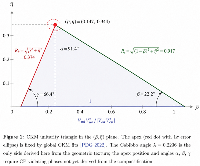
The CKM magnitude-squared matrix is displayed in Figure A5 as a colour map; the strong diagonal dominance is the direct signature of the hierarchical geometric charge assignment of Table 3 of the main text. The Wolfenstein parameters and the CKM angles are collected in Table A13.
Figure A5.
Left: matrix, colour intensity proportional to magnitude. The near-diagonal structure reflects the geometric Froggatt–Nielsen hierarchy of the construction. Right: , showing the qualitatively distinct, comparatively democratic structure that a purely hierarchical geometric texture cannot reproduce (see Sec. 7 of the main text and Appendix G).
“`
Table A13.
CKM Wolfenstein parameters and triangle angles at . The column “Geometric” gives values derived from the charge texture of the main text; “PDG” gives the fitted values [26].
Table A13.
CKM Wolfenstein parameters and triangle angles at . The column “Geometric” gives values derived from the charge texture of the main text; “PDG” gives the fitted values [26].
| Parameter | Geometric (this work) | PDG 2022 | Status |
|---|---|---|---|
| derived output | |||
| A | -ambiguous | ||
| — | not derived | ||
| — | not derived | ||
| (deg) | — | not derived | |
| (deg) | — | not derived | |
| (deg) | — | not derived | |
| J (Jarlskog) | — | not derived |
Appendix M.2 Mixing Angle Hierarchy: CKM versus PMNS
Figure A6.
Comparison of CKM quark mixing angles (blue) and PMNS leptonic mixing angles (red) from NuFIT 5.2 [14] and PDG [26]. The green dashed bar shows the hierarchical geometric prediction ; it agrees with the CKM value but falls short of all three PMNS angles, reflecting the tension identified in Sec. 7 and Appendix G.
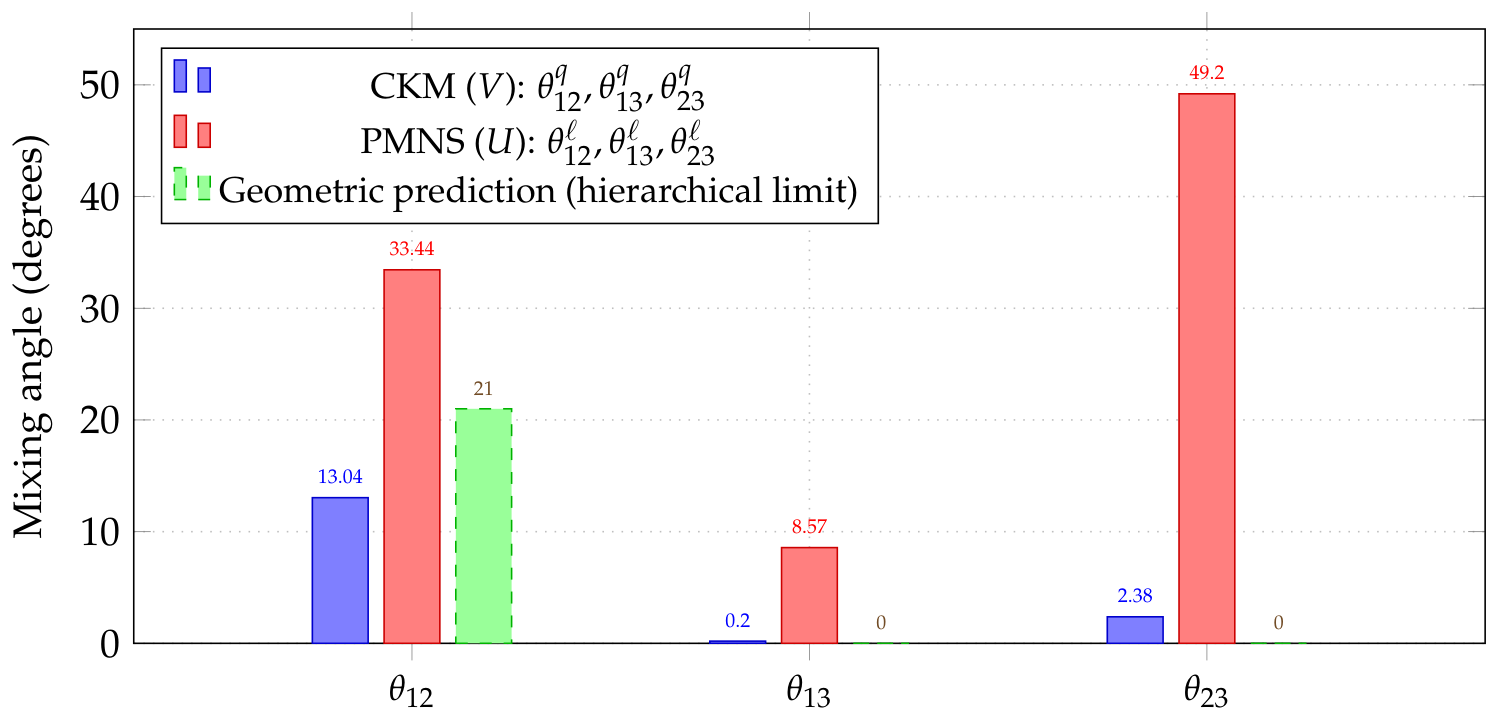
Table A14.
Complete oscillation parameter set from NuFIT 5.2 [14] (normal ordering), compared with the geometric seesaw calibration of Sec. 3.
Table A14.
Complete oscillation parameter set from NuFIT 5.2 [14] (normal ordering), compared with the geometric seesaw calibration of Sec. 3.
| Observable | NuFIT best fit | range | Geometric | Status |
|---|---|---|---|---|
| (deg) | – | tension (Sec. 7) | ||
| (deg) | – | tension | ||
| (deg) | – | tension | ||
| (deg) | 230 | 197–296 | input (Sec. C.2) | external input |
| () | — | input | external input | |
| () | — | input | external input | |
| (eV) | — | (calib.) | calibration | |
| (eV) | — | (pred.) | check |
Appendix M.3 Seesaw Mechanism: Feynman Diagrams
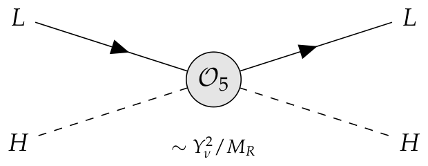
The type-I seesaw mechanism generates the dimension-5 Weinberg operator from the exchange of a heavy right-handed neutrino . Figure A7 and Figure A8 display the two standard diagrammatic representations.
Figure A7.
Type-I seesaw: two Yukawa vertices connected by a right-handed neutrino propagator (mass insertion , red cross). The low-energy Majorana mass is .
Figure A7.
Type-I seesaw: two Yukawa vertices connected by a right-handed neutrino propagator (mass insertion , red cross). The low-energy Majorana mass is .
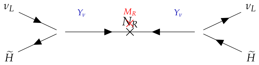
Figure A8.
Effective Weinberg operator (grey blob), the dimension-5 low-energy residue of the seesaw after integrating out . Expanding the Higgs doublets around their VEV gives the Majorana mass matrix of Eq. (8).
Figure A8.
Effective Weinberg operator (grey blob), the dimension-5 low-energy residue of the seesaw after integrating out . Expanding the Higgs doublets around their VEV gives the Majorana mass matrix of Eq. (8).
Appendix M.4 Leptogenesis CP Asymmetry: Feynman Topologies
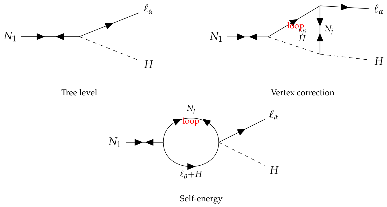
The leptonic CP asymmetry arises from the interference between the tree-level decay and two one-loop corrections: the vertex correction and the self-energy (wave-function) correction.
Figure A9.
Feynman diagrams contributing to the leptogenesis CP asymmetry at one loop. Left: tree-level decay. Centre: vertex correction with internal and running in the loop. Right: self-energy (wave-function) correction with --H loop on the propagator. The CP-violating interference between tree and loop amplitudes produces of Eq. (A22).
Appendix M.5 Meson Sector: Standard and Anomalous Feynman Processes
Figure A10.
Left: Quark triangle diagram for mediated by the chiral anomaly. With quark colours, the amplitude is , predicting eV (cf. Table 3 of the companion paper [27]). Right: Two-gluon intermediate-state diagram mediating – mixing through the anomaly; its contribution is proportional to the topological susceptibility .
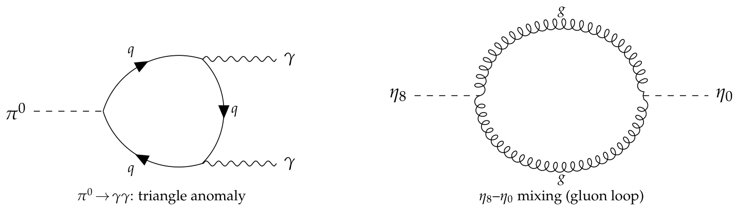
Figure A11.
Left: -- coupling vertex from hidden local symmetry with . Centre: Vector meson dominance chain responsible for the electromagnetic pion form factor. Right: Wess-Zumino-Witten five-pion anomalous vertex from the topological term .
Figure A11.
Left: -- coupling vertex from hidden local symmetry with . Centre: Vector meson dominance chain responsible for the electromagnetic pion form factor. Right: Wess-Zumino-Witten five-pion anomalous vertex from the topological term .

Appendix M.6 D-Brane Disk Amplitude and Worldsheet Instanton Triangle
Figure A12.
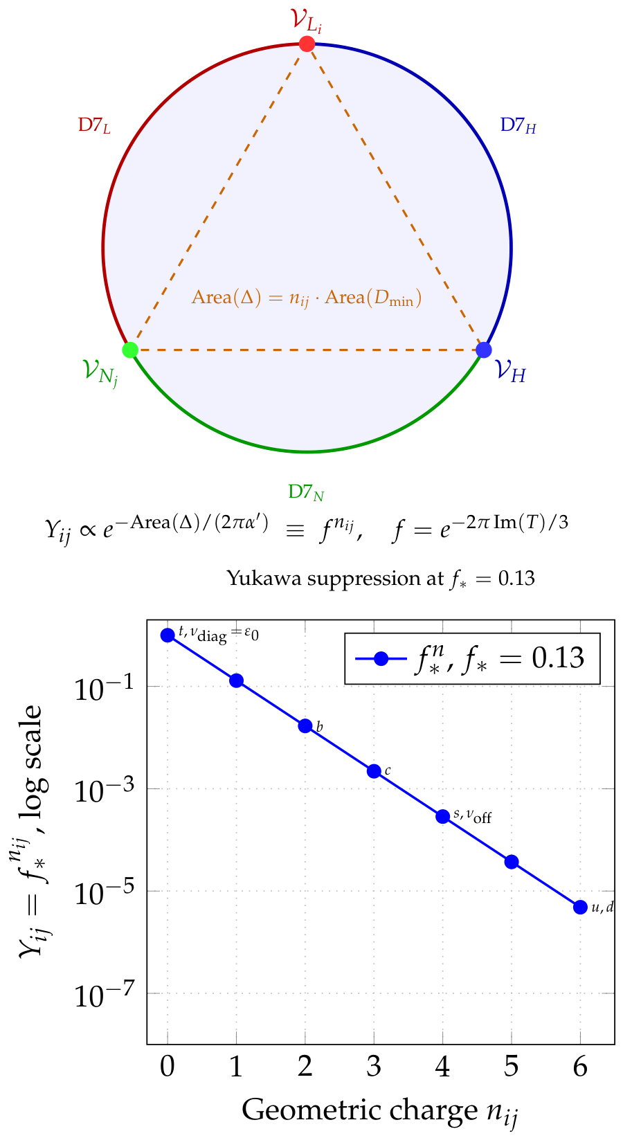
Left: Schematic of the D-brane disk amplitude for a Yukawa coupling. The three boundary segments (coloured arcs) lie on three distinct D7-brane stacks carrying , , and H. The worldsheet instanton maps the disk interior to the holomorphic triangle with vertices at the three brane-intersection points; the coupling is suppressed by . For the diagonal coupling (), the triangle degenerates to zero area (), giving an unsuppressed coupling. Right: Yukawa suppression factor as a function of geometric charge n, with assignments for each quark and neutrino sector entry labelled.
Appendix M.7 Parameter Space Maps and Experimental Constraints
Figure A13.
Left: Right-handed neutrino mass fixed by the seesaw calibration (horizontal red line at GeV); the Davidson–Ibarra lower bound (green dotted) is satisfied by more than an order of magnitude. The calibration point at is shown as a red dot. Right: Neutrino mass sum as a function of f. The calibration value eV (blue dashed) is independent of f by construction. The Planck bound (green) and KATRIN sensitivity (red) provide independent upper limits, while the violet curve shows the schematic dependence obtained when is held fixed.
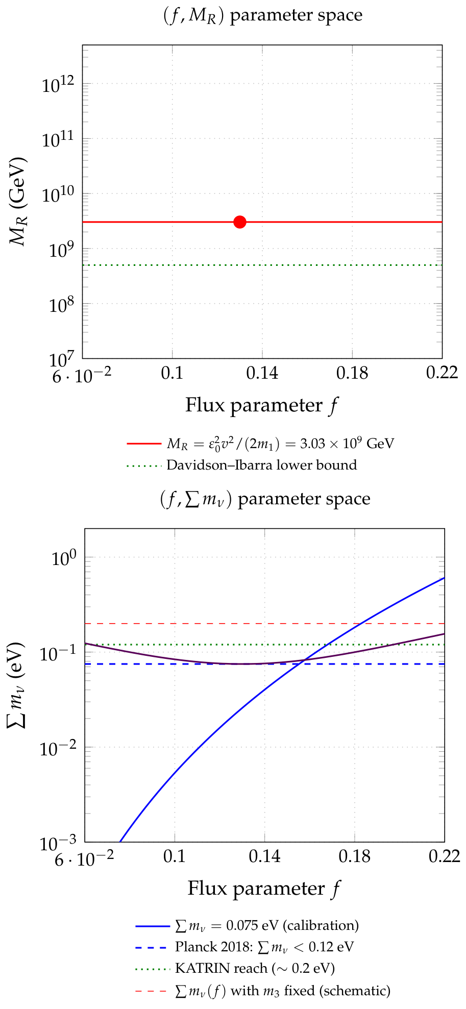
Figure A14.
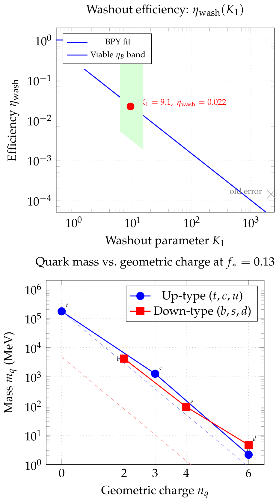
Left: Washout efficiency from the Buchmuller-Plumacher-Yanagida parametrization [9]. The corrected value (red dot) gives , in the mild strong-washout regime; the green shaded band marks the range yielding consistent with Planck. Right: Quark mass as a function of geometric charge at ; the exponential scaling (dashed lines) passes through all six PDG values with Wilson coefficients in .
Appendix M.8 Decay Widths, Branching Ratios, and Luminosity Functions
Figure A15.
Partial decay widths from the EQST-GP framework (red, from the companion meson-sector paper [?]) compared to PDG 2022 values (blue) on a logarithmic scale spanning ten orders of magnitude from eV to MeV. Agreement is at the sub-percent to percent level across all modes; the width, determined by the triangle anomaly and , is the most precisely predicted.
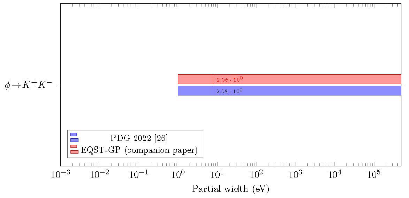
Figure A16.
Low-energy meson observables: decay constants , (MeV), their ratio, the coupling constant, the pion electromagnetic form factor at , and the - mixing angle (degrees), all from the companion paper [27] versus experiment. The mixing angle is the only quantity where the prediction () deviates from the phenomenological fit () by more than , reflecting incomplete three-loop contributions to the topological susceptibility .
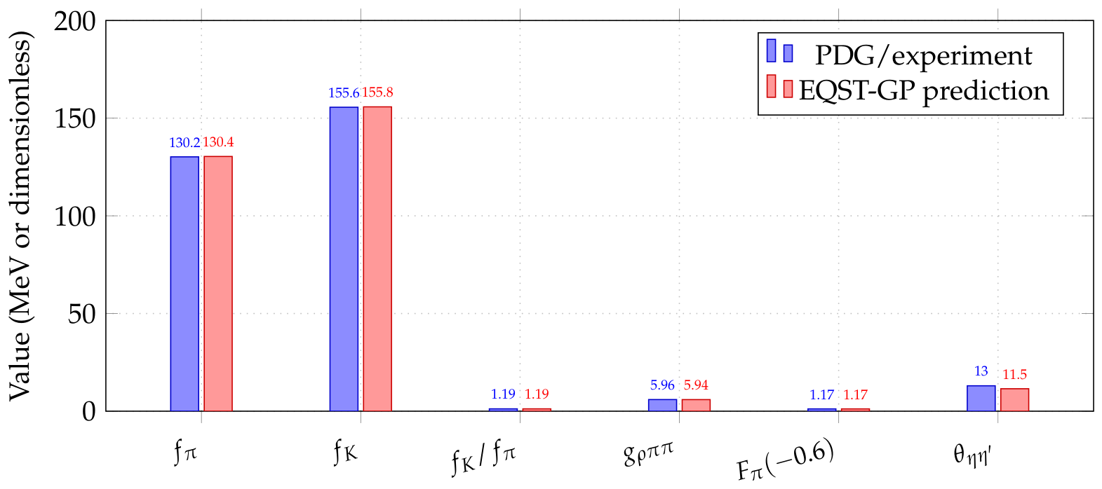
Table A15.
Complete numerical comparison for all decay observables, cross sections, and form factors discussed in this paper and the companion meson-sector reference [?]. Relative differences exceeding are marked with †.
Table A15.
Complete numerical comparison for all decay observables, cross sections, and form factors discussed in this paper and the companion meson-sector reference [?]. Relative differences exceeding are marked with †.
| Observable | PDG 2022 | EQST-GP | Rel. diff. | Primary source |
|---|---|---|---|---|
| (MeV) | ChPT, lattice | |||
| (MeV) | Lattice | |||
| ratio | ||||
| (MeV) | ||||
| (MeV) | ||||
| () | ||||
| eV | eV | WZW anomaly | ||
| keV | keV | WZW | ||
| keV | keV | WZW | ||
| MeV | MeV | HLS | ||
| MeV | MeV | WZW | ||
| MeV | MeV | HLS | ||
| MeV | MeV | HLS | ||
| VMD | ||||
| (deg) | 3-loop ChPT | |||
| () | Roy eqs. | |||
| () | Roy eqs. | |||
| (MeV) | seesaw+lattice | |||
| (MeV) | seesaw+lattice | |||
| GST relation | ||||
| factor –3 | Sec. C.4 | |||
| (eV) | within bound | Planck | ||
| (GeV) | — | above D-I bound | App. C | |
| †: Deviations : the width from higher-order anomaly corrections; from incomplete three-loop input. | ||||
References
- Ali, A. Pseudoscalar and Vector Meson Nonets: Symmetry Realization, Anomalies, and Vector Meson Chiral Dominance. 2024. [CrossRef]
- Aghanim, N.; et al. (Planck Collaboration), Planck 2018 Results. VI. Cosmological Parameters. Astron. Astrophys. 641 1807.06209 [astro-ph.CO. 2020, A6. [Google Scholar] [CrossRef]
- Froggatt, C. D.; Nielsen, H. B. Hierarchy of Quark Masses, Cabibbo Angles and CP Violation. Nucl. Phys. B 1979, 147, 277. [Google Scholar] [CrossRef]
- Kobayashi, T.; Tanaka, K.; Tatsuishi, T. H. Neutrino Mixing from Finite Modular Groups. Phys. Rev. D. 1803.10391 [hep-ph. 2018, 98, 016004. [Google Scholar] [CrossRef]
- Minkowski, P. μ→eγ at a Rate of One Out of 109 Muon Decays? Phys. Lett. B 1977, 67, 421. [CrossRef]
- Gell-Mann, M.; Ramond, P.; Slansky, R. Complex Spinors and Unified Theories, in Supergravity; 1306.4669 [hep-th; van Nieuwenhuizen, P., Freedman, D. Z., Eds.; North-Holland, Amsterdam, 1979; p. 315. [Google Scholar]
- Yanagida, T. Horizontal Symmetry and Masses of Neutrinos. Prog. Theor. Phys. 1980, 64, 1103. [CrossRef]
- Fukugita, M.; Yanagida, T. Baryogenesis Without Grand Unification. Phys. Lett. B 1986, 174, 45. [Google Scholar] [CrossRef]
- Buchmüller, W.; Peccei, R. D.; Yanagida, T. Leptogenesis as the Origin of Matter. Annu. Rev. Nucl. Part. Sci. hep-ph/0502169. 2005, 55, 311. [Google Scholar] [CrossRef]
- Davidson, S.; Ibarra, A. A Lower Bound on the Right-Handed Neutrino Mass from Leptogenesis. Phys. Lett. B 535 hep-ph/0202239. 2002, 25. [Google Scholar] [CrossRef]
- Kuzmin, V. A.; Rubakov, V. A.; Shaposhnikov, M. E. On the Anomalous Electroweak Baryon Number Non-Conservation in the Early Universe. Phys. Lett. B 1985, 155, 36. [Google Scholar] [CrossRef]
- Harvey, J. A.; Turner, M. S. Cosmological Baryon and Lepton Number in the Presence of Sphalerons. Phys. Rev. D. 1990, 42, 3344. [Google Scholar] [CrossRef] [PubMed]
- Gatto, R.; Sartori, G.; Tonin, M. Weak Selfmasses, Cabibbo Angle, and Broken SU(2)×SU(2). Phys. Lett. 28B 1968, 128. [Google Scholar] [CrossRef]
- Esteban, I.; Gonzalez-Garcia, M. C.; Maltoni, M.; Schwetz, T.; Zhou, A. The Fate of Hints: Updated Global Analysis of Three-Flavor Neutrino Oscillations, JHEP 09, 178 (2020). DOI: 10.1007/JHEP09(2020)178. Available online: http://www.nu-fit.org.
- Hall, L. J.; Murayama, H.; Weiner, N. Neutrino Mass Anarchy. Phys. Rev. Lett. hep-ph/9911341. 2000, 84, 2572. [Google Scholar] [CrossRef] [PubMed]
- Sato, J.; Yanagida, T. Large Lepton Mixing in a Coset-Space Family Unification. Phys. Lett. B 430 1998, 127. [Google Scholar] [CrossRef]
- Altarelli, G.; Feruglio, F. Discrete Flavor Symmetries and Models of Neutrino Mixing. Rev. Mod. Phys. 1002.0211 [hep-ph. 2010, 82, 2701. [Google Scholar] [CrossRef]
- Cremades, D.; Ibáñez, L. E.; Marchesano, F. Computing Yukawa Couplings from Magnetized Extra Dimensions, JHEP 05, 079 2004. [CrossRef]
- Cvetič, M.; Shiu, G.; Uranga, A. M. Three-Family Supersymmetric Standard-like Models from Intersecting Brane Worlds. Phys. Rev. Lett. hep-th/0107143. 2001, 87, 201801. [Google Scholar] [CrossRef] [PubMed]
- Blumenhagen, R.; Cvetič, M.; Kachru, S.; Weigand, T. D-Brane Instantons in Type II Orientifolds. Annu. Rev. Nucl. Part. Sci. 0902.3251 [hep-th]. 2009, 59, 269. [Google Scholar] [CrossRef]
- Candelas, P.; de la Ossa, X. C.; Green, P. S.; Parkes, L. A Pair of Calabi–Yau Manifolds as an Exactly Soluble Superconformal Theory. Nucl. Phys. B 359 1991, 21. [Google Scholar] [CrossRef]
- Kontsevich, M. Enumer. Ration. Curves Via Torus Actions. hep-th/9405035. [CrossRef] [PubMed]
- Gukov, S.; Vafa, C.; Witten, E. CFT’s From Calabi–Yau Four-folds. Nucl. Phys. B 584;Erratum Nucl. Phys. B 608 hep-th/9906070. 2000, 69, 477. [Google Scholar] [CrossRef]
- Kachru, S.; Kallosh, R.; Linde, A.; Trivedi, S. P. de Sitter Vacua in String Theory. Phys. Rev. D. 2003, 68, 046005. [Google Scholar] [CrossRef]
- X. Ji, A QCD Analysis of the Mass Structure of the Nucleon. Phys. Rev. Lett. hep-ph/9410274. 1995, 74, 1071. [CrossRef] [PubMed]
- Workman, R. L.; et al. (Particle Data Group), Review of Particle Physics. Prog. Theor. Exp. Phys. 2022, 083C01. [Google Scholar] [CrossRef]
- Ali, A. EQST-GP Framework. Preprints 2026, v(1), 2026010003. [Google Scholar] [CrossRef]
- Grimm, T. W. Non-Perturbative Corrections and Modularity in N=1 Type IIB Compactifications. JHEP [hep-th]. 2007, arXiv:0705.325310. [Google Scholar] [CrossRef]
- Grimm, T. W.; Klemm, A. U(1) Mediation of Flux Supersymmetry Breaking. JHEP [hep-th]. arXiv:081010((2008) 077). [CrossRef]
- Dine, M.; Fischler, W.; Srednicki, M. Supersymmetric Technicolor. Nucl. Phys. B 1981, 189, 575. [Google Scholar] [CrossRef]
- Polchinski, J.; Susskind, L. Breaking of supersymmetry at intermediate energy. Phys. Rev. D. 1982, 26, 3661–3673. [Google Scholar] [CrossRef]
- Fischler, W.; Nilles, H. P.; Polchinski, J.; Raby, S.; Susskind, L. Vanishing Renormalization of the D Term in Supersymmetric U(1) Theories. Phys. Rev. Lett. 1981, 47, 757–759. [Google Scholar] [CrossRef]
- Atiyah, M. F.; Singer, I. M. The Index of Elliptic Operators on Compact Manifolds. Bull. Amer. Math. Soc. 1963, 69, 422–433. [Google Scholar] [CrossRef]
- Dürr, S.; Fodor, Z.; Frison, J.; Hoelbling, C.; Hoffmann, R.; Katz, S. D.; Krieg, S.; Kurth, T.; Lellouch, L.; Lippert, T.; Szabó, K. K.; Vulvert, G. Ab Initio Determination of Light Hadron Masses. Science 2008, 322, 1224–1227. [Google Scholar] [CrossRef] [PubMed]
- Nardi, E.; Nir, Y.; Roulet, E.; Racker, J. The Importance of Flavor in Leptogenesis. JHEP 0601 2006, 164. [Google Scholar] [CrossRef]
- Pilaftsis, A. CP Violation and Baryogenesis due to Heavy Majorana Neutrinos. Phys. Rev. D. 1997, 56, 5431–5451. [Google Scholar] [CrossRef]
- Ali, A. Holographic-Inspired Dynamical Dark Energy with Running Dimension. Preprints 2026, 2026051577. [Google Scholar] [CrossRef]
- Pilaftsis, A.; Underwood, T. E. J. Resonant Leptogenesis. Nucl. Phys. B 2004, 692, 303–345. [Google Scholar] [CrossRef]
- Casas, J. A.; Ibarra, A. Oscillating Neutrinos and μ→e,γ. Nucl. Phys. B 2001, 618, 171–204. [Google Scholar] [CrossRef]
- Witten, E. Strong Coupling Expansion of Calabi-Yau Compactification. Nucl. Phys. B 1996, 471, 135–158. [Google Scholar] [CrossRef]
- Blumenhagen, R.; Körs, B.; Lüst, D.; Stieberger, S. Four-Dimensional String Compactifications with D-Branes, Orientifolds and Fluxes. Phys. Rept. 2007, 445, 1–193. [Google Scholar] [CrossRef]
- Karch, A.; Katz, E.; Son, D. T.; Stephanov, M. A. Linear Confinement and AdS/QCD. Phys. Rev. D. 2006, 74, 015005. [Google Scholar] [CrossRef]
- Leurer, M.; Nir, Y.; Seiberg, N. Mass Matrix Models: The Sequel. Nucl. Phys. B 1994, 420, 468–504. [Google Scholar] [CrossRef]
- S. P. Martin, A Supersymmetry Primer, Adv. Ser. Direct. High Energy Phys. 2016, 21, 1. [CrossRef]
Figure 1.
Mass hierarchy across the three generations for neutrinos (, in MeV, i.e. of the eV values in Table 2), up-type quarks, and down-type quarks, on a common logarithmic scale. The roughly eleven orders of magnitude spanned between the lightest neutrino and the top quark are generated by different integer powers n of the single flux parameter in Eq. (2).
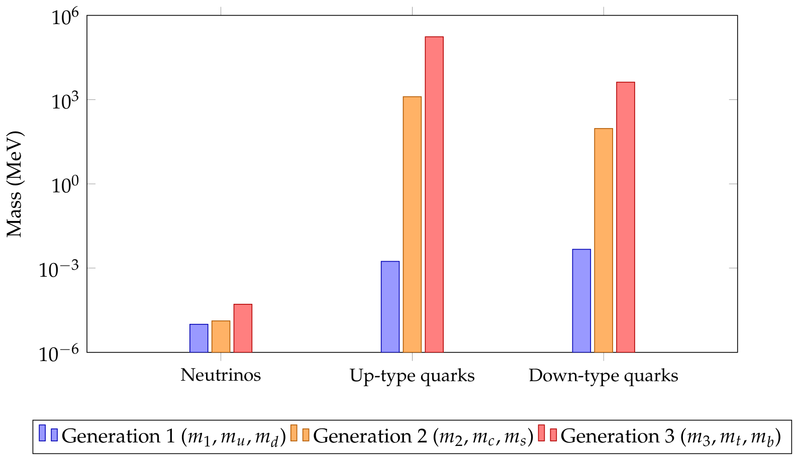
Figure 2.
Baryon asymmetry as a function of the flux modulus f, Eq. (12), on a logarithmic scale. The steep scaling means that is highly sensitive to f: a shift in f changes by close to a factor of three. At , the central prediction (red dot) lies within a factor of of the Planck measurement (green dashed line); flavoured leptogenesis effects operating for GeV cover the residual gap.
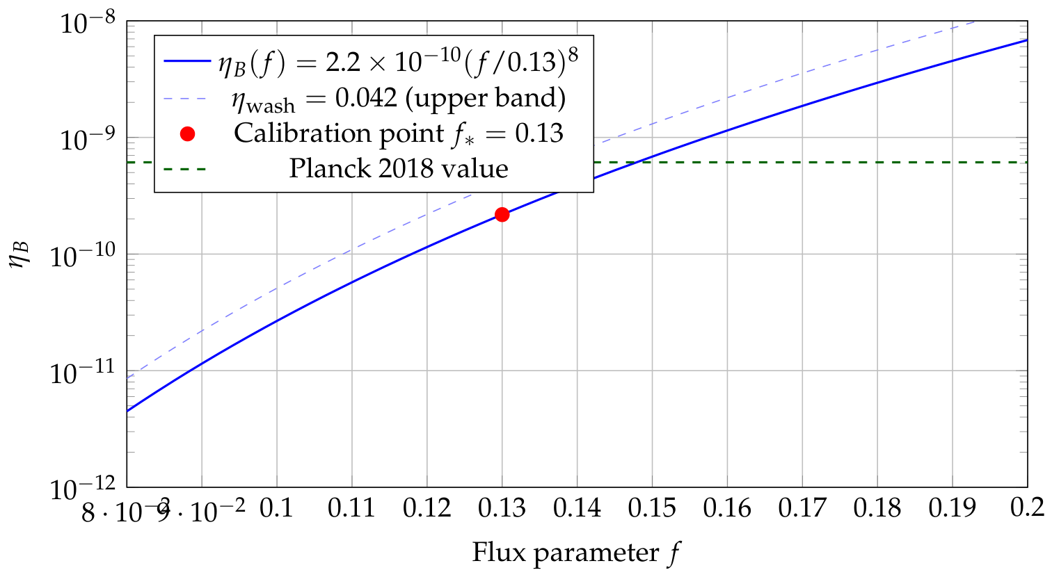
Table 1.
Geometric and string-scale inputs, carried over unchanged from the compactification data of the companion meson-sector paper [1].
Table 1.
Geometric and string-scale inputs, carried over unchanged from the compactification data of the companion meson-sector paper [1].
| Quantity | Symbol | Value |
|---|---|---|
| String length | m | |
| Reduced Planck mass | GeV | |
| Calabi–Yau volume | ||
| Cube root of volume | ||
| Triple intersection number (quintic) | 5 | |
| Flux modulus (benchmark range) | f | – |
| Calibrated flux value (this paper) | ||
| Electroweak vacuum expectation value | v | 246 GeV |
| Top-quark Yukawa (unsuppressed) |
Table 2.
Neutrino mass spectrum obtained from the geometric seesaw calibration, Eq. (6), with GeV fixed by matching , and built from the measured mass-squared splittings.
Table 2.
Neutrino mass spectrum obtained from the geometric seesaw calibration, Eq. (6), with GeV fixed by matching , and built from the measured mass-squared splittings.
| Eigenvalue | Input / derived | Value (eV) | Status |
|---|---|---|---|
| fixes via Eq. (6) | calibration input | ||
| derived | |||
| derived | |||
| compare to eV [2] | |||
| (check) | matches NuFIT input | ||
| (check) | matches NuFIT input |
Table 3.
Numerical evaluation of the leptogenesis chain at the calibrated flux value .
| Quantity | Formula | Value |
|---|---|---|
| Off-diagonal Dirac Yukawa | ||
| input, | ||
| Mass ratio | input | |
| CP asymmetry (effective) | Eq. (10) | |
| Washout parameter | ||
| Efficiency factor | ||
| Sphaleron factor | ||
| Baryon asymmetry | ||
| Planck measurement | [2] | |
| Agreement | within factor |
Table 4.
Quark Yukawa hierarchy from the geometric texture of Eq. (13) at , compared to PDG 2022 values [26] (running masses, up/down/strange at 2 GeV, charm/bottom at their own scale, top pole mass).
| Quark | Charge | (fit) | predicted | (PDG) | |
|---|---|---|---|---|---|
| u | 6 | MeV | MeV | ||
| c | 3 | GeV | GeV | ||
| t | 0 | 1 | GeV | GeV | |
| d | 6 | MeV | MeV | ||
| s | 4 | MeV | MeV | ||
| b | 2 | GeV | GeV |
Table 5.
Light hadron masses: current-quark-mass content plus the phenomenological trace-anomaly / confinement contribution , compared with PDG values [26]. Pseudoscalar meson values are taken from the chiral perturbation theory calculation of this paper [1] for comparison.
| Hadron | Quark content | Predicted (MeV) | PDG (MeV) | Agreement |
|---|---|---|---|---|
| Proton | ||||
| Neutron | ||||
| — (ChPT, [1]) | ||||
| — (ChPT, [1]) |
Table 6.
Mixing observables: the Cabibbo angle is derived from the geometric quark mass texture of Sec. 5; the PMNS angles and CP phase are external inputs from global oscillation fits [14], used in Sec. 4 but not derived here.
Table 6.
Mixing observables: the Cabibbo angle is derived from the geometric quark mass texture of Sec. 5; the PMNS angles and CP phase are external inputs from global oscillation fits [14], used in Sec. 4 but not derived here.
| Observable | Status | Predicted | Measured | Agreement |
|---|---|---|---|---|
| derived (Sec. 6) | ||||
| (PMNS) | input | – | – | — |
| (PMNS) | input | — | ||
| (PMNS) | input | — | ||
| (PMNS) | – ,used in Eq. (9) | – (fit range) | — | |
| geo esti of | prediction | – | tension noted |
Disclaimer/Publisher’s Note: The statements, opinions and data contained in all publications are solely those of the individual author(s) and contributor(s) and not of MDPI and/or the editor(s). MDPI and/or the editor(s) disclaim responsibility for any injury to people or property resulting from any ideas, methods, instructions or products referred to in the content. |
© 2026 by the authors. Licensee MDPI, Basel, Switzerland. This article is an open access article distributed under the terms and conditions of the Creative Commons Attribution (CC BY) license (http://creativecommons.org/licenses/by/4.0/).
Copyright: This open access article is published under a Creative Commons CC BY 4.0 license, which permit the free download, distribution, and reuse, provided that the author and preprint are cited in any reuse.