

Submitted:
19 September 2026
Posted:
20 September 2026
You are already at the latest version
Abstract
Range anxiety among electric vehicle (EV) drivers stems less from battery capacity itself than from the difficulty of trusting a dashboard range estimate and choosing, quickly, among charging options of unequal speed, price and compatibility. The authors' earlier work encoded this choice as a Boolean Satisfiability problem solved once, offline, using a fixed energy-consumption rate on short intra-city routes. This paper extends that formulation to Predictive Constraint-Verified EV Routing (PC-EVR), a system that (i) predicts a vehicle's achievable range from live telemetry using a trained XGBoost regressor rather than a fixed rate, and (ii) re-solves the next charging decision at every real stop as a Weighted Partial MaxSAT instance, using the RC2 core-guided solver, in which a 20% state-of-charge floor is a non-negotiable constraint that filters candidates outright rather than a factor the solver merely weighs in. The range predictor is selected after a controlled, identical-split comparison against Linear Regression, Random Forest and a neural network, and its selection is validated by a dedicated ablation study rather than an offline error metric alone. PC-EVR is benchmarked against two purpose-built greedy baselines (nearest-station, cheapest-station) under identical safety and traffic assumptions, across five real long-distance Indian trips and India's national government charging-station registry of 39,641 stations. The proposed system completes every trip without a single safety-constraint violation while reducing average trip time by approximately 8.7 hours against the nearest-station baseline and 21.6 hours against the cheapest-station baseline. The ablation study further shows that routing quality is insensitive to small prediction-accuracy differences among tree- and network-based models but degrades measurably once accuracy falls below a threshold, a finding with direct implications for range-model selection in future systems.
Keywords:
electric vehicles
; charging station recommendation
; route optimization
; Weighted Partial MaxSAT
; RC2 solver
; XGBoost
; range prediction
; State of Charge
; real-time optimization
1. Introduction
The number of electric vehicles on Indian roads has grown quickly over the past several years, yet a basic uncertainty still accompanies most long trips: whether the displayed range will hold up over the remaining distance, and which of several nearby charging options is actually worth a detour. Battery technology and public charging infrastructure have both improved substantially [1], but the software layer that is supposed to connect a vehicle's real-time state to a specific, defensible charging decision has not kept pace with either. Survey and review literature consistently identifies this uncertainty commonly termed range anxiety as one of the more persistent barriers to EV adoption [2,3], and its root cause is less a shortage of battery capacity than a lack of trust in the number shown to the driver and a lack of a principled way to act on it while already on the road.
A manufacturer-rated range figure is typically obtained under standardized, low-speed test conditions and can diverge substantially from what a vehicle actually delivers at highway speed and in hot ambient conditions, since aerodynamic drag, climate-control load and battery efficiency all shift with speed and temperature. A driver who plans a multi-hundred-kilometre trip around the rated figure alone can therefore find, part-way through the journey, that the remaining charge covers far less distance than expected, forcing a sequence of ad hoc, incompletely informed charging-stop decisions under time pressure. This is not a failure of judgement on the driver's part; it is an accurate description of a combinatorial decision problem choosing which stations to visit, in what order, and how much to charge at each being solved by hand, one stop at a time, with incomplete information about both the vehicle's true state and the consequence of each choice for the stops that follow.
Four broad families of method have been applied to some version of this problem. Exact mathematical programming linear and mixed-integer formulations can represent the problem rigorously but is used almost exclusively for offline infrastructure-siting decisions rather than live, single-trip routing, since solving to provable optimality is too slow to repeat every time a vehicle's state of charge changes en route, and such formulations tend to require a thicket of auxiliary constraints to express purely logical requirements such as connector compatibility [4,8,9]. Metaheuristics genetic algorithms, ant-colony optimization, tabu search and related methods scale to larger instances than exact solvers but provide no optimality guarantee, and their solution quality depends on hand-tuned parameters that typically need re-tuning for each new problem instance. Reinforcement-learning and bandit approaches can adapt online but need substantial training data or a high-fidelity simulator, and the resulting policy is effectively a black box, offering no way to certify in advance that a recommended route will never leave the vehicle below a safe charge level. Finally, the single-objective greedy heuristics that most commercial navigation tools fall back on always route to the closest charger, or always route to whichever option is cheapest are simple and quick to reason about, but each judges a station on only one attribute and has no way to account for how that pick narrows the choices available at the next stop.
Boolean Satisfiability (SAT) and its weighted optimization generalization, Maximum Satisfiability (MaxSAT), offer a different route into this problem: real-world requirements such as state-of-charge limits, charger compatibility and route continuity can be expressed directly as logical clauses in Conjunctive Normal Form and processed with modern solvers, separating constraints that must always hold from preferences that should be satisfied as well as possible [6]. The authors previously formulated intercity EV charging-station selection along these lines, encoding distance, cost and compatibility constraints as CNF clauses solved with Google OR-Tools' CP-SAT solver, and reported solve times as low as 0.01 seconds together with lower distance, energy and cost than a Linear Programming baseline across several short Hyderabad routes of 5–47 km [1]. That study established that logic-based combinatorial solving is well suited to this class of constraint-heavy selection problem, but it treated energy consumption as a single fixed input supplied ahead of time, solved the station-selection problem once per trip rather than repeatedly, and was validated only at intra-city scale.
Two limitations of that formulation matter once the trip scale grows from an intra-city hop to an interstate journey of several hundred kilometres. First, a fixed consumption rate is a reasonable simplification over a short, predictable route but becomes systematically wrong over a longer one, where speed, ambient temperature, terrain and the battery's own state of charge all vary enough to shift real energy use substantially from any single assumed rate. Second, a plan computed once at the start of the trip cannot be corrected once conditions diverge from that initial assumption, since nothing in a one-shot formulation re-evaluates the decision as the vehicle's actual state evolves. The present study addresses both limitations directly, and does so at a validation scale five real interstate trips run against India's national government charging-station registry that stresses the routing problem in a way a handful of short intra-city test routes does not. Beyond the authors' own prior formulation, it is also worth situating this work against the recent emergence of commercial-scale EV trip planning: in March 2026, Google introduced an AI-based EV trip planner for Android Auto that predicts battery usage from vehicle weight, battery size, live traffic, elevation and weather across more than 350 vehicle models [24]. This is useful evidence that the underlying problem is commercially significant, though the feature's coverage of Indian EV models was not confirmed at the time of writing, and its underlying method, being proprietary, cannot be independently benchmarked or verified a transparency gap this work is positioned to help close for the Indian market rather than to claim outright superiority over a system that has not been evaluated on the same trips.
This paper makes four contributions relative to the authors' earlier SAT/CP-SAT formulation and to the broader literature reviewed above. It replaces the fixed consumption-rate assumption with a range predictor trained on live telemetry and selected through a controlled comparison against three alternative model families, with the selection independently validated by an ablation study rather than assumed from an offline accuracy figure alone. It reformulates station selection as a Weighted Partial MaxSAT problem solved with the RC2 core-guided solver, in which the safety-critical state-of-charge floor is a hard constraint excluded from the search outright rather than one term in a combined score, and in which the decision is re-solved at every real stop using the vehicle's actual measured state rather than fixed once at departure. It introduces two purpose-built, deliberately naive baseline systems that share every assumption with the proposed system except the decision strategy itself, so that a measured difference in outcome can be attributed to the strategy rather than to an incidental advantage. Finally, it benchmarks all three systems against a national-scale charging-station registry rather than a synthetic or small dataset, and reports the resulting comparison including the conditions under which a naive baseline can still perform competitively candidly rather than selectively.
The remainder of this paper is organized as follows. Section 2 describes the problem formulation, the machine-learning range predictor, the Weighted Partial MaxSAT encoding, the baseline systems and the datasets and experimental protocol used to evaluate them. Section 3 reports the range-prediction accuracy comparison, the range-model ablation study, and the system-level benchmark results. Section 4 discusses the mechanism behind these results, situates them against the authors' prior work and against commercial systems, and states the limitations of the present study candidly. Section 5 concludes and outlines directions for future work.
2. Materials and Methods
PC-EVR is organized as four stages that each do one job and can be tested independently: estimate the vehicle's currently achievable range, turn the routing decision into a Weighted Partial MaxSAT instance, hand that instance to RC2 for solving, and surface the recommendation through a web interface before looping back to the first stage at the vehicle's next real stop rather than terminating after one pass. Figure 3 summarizes this architecture and highlights the feedback loop that distinguishes it from a one-shot formulation.
2.1. Problem Formulation
The routing environment is represented as a directed graph G = (V, E) (Eq. 1), where V = {v0, v1, …, vn} denotes the trip origin, the destination, and the set of candidates charging stations along the corridor, and E ⊆ V × V is the set of feasible road segments between them. For an edge (i, j) ∈ E, dij denotes the travel distance in kilometres, tij the travel time in hours under the applicable traffic multiplier (Section 2.6), and cij the energy consumed traversing the segment, computed from the range prediction described in Section 2.4. A candidate route is an ordered sequence P = {v0, v1, …, vk} (Eq. 2); unlike the authors' earlier formulation [1], the intermediate stops here are not fixed up front but are chosen and sequenced incrementally, one charging decision at a time, as the trip proceeds. At each decision point, a Boolean decision variable xi is introduced for every station i still under consideration, equal to 1 if station i is selected as the next stop and 0 otherwise (Eq. 3).
2.2. Hard Constraints
Four requirements are encoded as classical CNF clauses that must be satisfied by any feasible solution. State-of-charge feasibility requires that a selected station leave the vehicle at or above a safety floor on arrival, xi ⇒ (SOCarrive,i ≥ SOCfloor) (Eq. 4), with SOCfloor set at 20% of usable battery capacity; any candidate whose arrival SOC would fall under this threshold is removed from consideration before the solver runs at all, for every one of the three systems evaluated here, rather than being scored down and possibly still chosen. Charger compatibility requires xi ⇒ Ci (Eq. 5); Ci evaluates to true precisely when station i's connector is compatible with the vehicle being routed. No-redundant-visits excludes selecting the same physical station twice within a trip, ¬(xi ∧ xj) for any two decision points i, j representing one station (Eq. 6) a constraint that, in an earlier implementation, was omitted from the emergency fallback path and produced a station being offered back to the vehicle it had already visited, a failure mode corrected in the version evaluated here. A route-corridor constraint additionally requires a candidate station to lie within a bounded distance of the real routed polyline (1 km for trips under 50 km, 5 km for longer highway trips), rather than a straight-line approximation, so the search cannot suggest a technically reachable station that sits well off the actual driving corridor.
2.3. Weighted Soft-Clause Objective
Preferences the system should try to satisfy, but which a solution need not meet exactly, take the form of weighted soft clauses, combined into a single cost figure that the RC2 solver minimizes at each decision point:
Cost = wd·detour_km + wp·(1 − progress_km) + wt·time_penalty + wc·cost_kwh + wm·(1 − margin) (7)
Table 1 lists the five components together with the weight assigned to each and the rationale behind it. The weights were arrived at empirically rather than assumed: an earlier configuration that weighted distance-to-destination far more heavily than the other terms allowed a solver optimizing cost or distance alone to match the proposed system on its own metric almost by default, and a later configuration that weighted detour without a separate progress term produced several near-worthless stops clustered close to the trip origin, since a nearby station incurs almost no detour regardless of whether it meaningfully advances the trip. The final weighting in Table 1 removes both failure modes by giving progress toward the destination an explicit, separately weighted role.
2.4. Machine-Learning Range Prediction
The range predictor is trained on a 5,000-row telemetry dataset recording State of Charge (%), Voltage (V), Current (A), Temperature (°C), Speed (km/h) and Distance (km) for each observation, with Remaining Range (km) as the target. Because the original dataset's Distance feature covers only 0–300 km, while the interstate trips evaluated in Section 2.7 run into the thousands of kilometres, a second, clearly labelled synthetic extension of 5,000 rows was generated for the deployed model, drawing SOC, Current, Temperature and Speed from the same ranges as the real data, Distance from a non-overlapping 300–3000 km range, and Remaining Range from a generative model fitted to the real data with residual noise sampled from that model's own measured error distribution; a source column distinguishes real from synthetic_extension rows throughout. The identical-split accuracy comparison reported in Section 3.1 is deliberately restricted to the real-only data to keep that specific claim uncontaminated by synthetic rows.
Four candidate models were compared under an identical 80/20 holdout split (random_state = 42), so that no model is evaluated on an easier or harder set of rows than another: (i) Linear Regression, a single global linear fit across all features; (ii) Random Forest, an ensemble of independently grown decision trees whose predictions are averaged; (iii) a Multi-Layer Perceptron (MLP), a small feed-forward neural network trained on standardized inputs; and (iv) XGBoost, a gradient-boosted tree ensemble in which each new tree is trained specifically to correct the residual error left by the trees before it, with shallow trees, subsampling and a conservative learning rate applied for regularization. XGBoost was adopted as the production model (Section 3.1) and is re-queried at every charging decision within a trip, using the vehicle's actual measured telemetry at that moment, rather than once at departure.
2.5. Solver: Weighted Partial MaxSAT via RC2
Each implication xi ⇒ Ai is converted to CNF using the standard equivalence xi ⇒ Ai ≡ ¬xi ∨ Ai (Eq. 8), and conjunctive implications (xi ∧ yj) ⇒ Bk become ¬xi ∨ ¬yj ∨ Bk (Eq. 9) via the corresponding De Morgan transformation, following standard SAT-encoding practice [6]. The resulting hard-clause and weighted soft-clause sets together form a Weighted Conjunctive Normal Form (WCNF) instance, solved with RC2, a core-guided Weighted Partial MaxSAT solver exposed through the PySAT toolkit [10,13]. RC2 works by repeatedly locating sets of soft clauses that cannot all be satisfied at once (while every hard clause is still required to hold), and loosening each such set through auxiliary cardinality constraints until an assignment is found that satisfies every hard clause while minimizing the total weight of violated soft clauses [10,11,12]. Within one solved WCNF instance the returned assignment is exact with respect to Equation 7, subject to the hard constraints of Section 2.2.
2.6. Relaxation Ladder and Traffic Modelling
A purely hard-constrained search can occasionally find no candidate at all on a long corridor through a sparsely covered region, so the search relaxes through a graduated ladder rather than failing outright on the first, strictest attempt: availability and operating-hour constraints relax first, the minimum-progress requirement degrades in stages tied to remaining charge (Table 2), and the state-of-charge floor and route-corridor constraint are among the last requirements to give way. Table 2 also reflects that this urgency-scaled behaviour is shared identically across all three systems compared in this study, since it represents ordinary reachability planning rather than the differentiator under investigation; what differs between systems is purely which station is selected once a candidate clears this bar. Travel time is scaled by a handful of speed multipliers tied to time of day, chosen to reflect documented Indian urban congestion patterns [18,19] rather than a live traffic feed, applied identically across all three systems so a trip that happens to start during a congested period is simply slower for every system under comparison.
2.7. Baseline Systems
Two deliberately naive, purpose-built baselines were implemented to isolate the effect of the decision strategy itself, consistent with the practice of using greedy nearest-neighbour heuristics as the standard comparison point for more sophisticated routing methods [20,23]. Baseline 1 (Nearest-Station) evaluates every feasible, reachable, not-yet-visited station at each decision point and selects whichever is physically closest, using the vehicle manufacturer's own linear range formula (rated range multiplied by current state-of-charge percentage) the estimate most consumer dashboards and basic navigation applications actually display. Baseline 2 (Cheapest-Station) instead selects the reachable station with the lowest modelled cost per kWh, using a physics-informed static range heuristic that adjusts the manufacturer formula by fixed temperature and speed penalty terms. Both baselines share the proposed system's 20% hard SOC floor, charger-type-aware charge target, traffic multipliers, urgency-scaled progress thresholds (Table 2), route-corridor constraint, candidate-generation code and charging-station data; what is deliberately not shared is the proposed system's preference for DC fast-charging candidates and the multi-objective MaxSAT selection itself, since isolating exactly that difference is the purpose of the comparison.
2.8. Datasets
Three datasets underlie the evaluation. The vehicle specification table (Table 3 shows a representative sample) covers thirty verified Indian EV models, spanning the MG Comet EV (17.3 kWh, 230 km rated range) to the Mercedes-Benz EQS 580 (107.8 kWh, 857 km rated range), each with battery capacity, rated range and supported connector type recorded. The charging-station registry used for the benchmark in Section 3.4 is a cleaned version of the national “State, District, City and Location wise Electric Vehicle (EV) Charging Stations in India” dataset published by the Bureau of Energy Efficiency, Ministry of Power, Government of India [25], comprising 39,641 station records across 5,902 cities, of which 69.7% offer AC charging and 30.3% offer DC fast charging, spanning operators including IOCL, UJOY, BPCL, Reliance BP and Tata Power among others. This registry does not include a pricing field, so a per-kWh cost is instead assigned computationally, varying by charger power and by whether the listed operator is a government or private entity, using publicly reported Indian charging-tariff bands as a guide (approximately ₹8–15 per kWh at private AC points, ₹15–25 per kWh at private DC fast chargers, and ₹4.5–7.5 per kWh where charging is government-regulated). Every cost figure reported in Section 3 should accordingly be read as this modelled estimate rather than a directly measured tariff. The telemetry dataset used to train the range predictor is described in Section 2.4.
2.9. Experimental Setup
All three systems were evaluated on five fixed real Indian interstate trips, chosen to span a range of distances, battery sizes and starting states of charge rather than to favour any one system (Table 4). Five metrics were recorded per trip: the number of charging stops, total detour distance relative to the direct route, traffic-adjusted total trip time (driving plus dwell time at every stop), total modelled charging cost, and trip-completion rate. All components ran inside a Google Colab notebook and were exposed to the user through an interactive Streamlit application; OpenRouteService [22] supplied routing, geocoding and route-leg distances, PySAT's RC2 implementation [10,13] solved the MaxSAT layer, and XGBoost [14] provided range prediction, with scikit-learn's Linear Regression and Random Forest used as comparison models.
3. Results
3.1. Range-Prediction Accuracy Comparison
Table 5 reports Root Mean Squared Error (RMSE), Mean Absolute Error (MAE) and the coefficient of determination (R²) for all four candidate models on the held-out test split. XGBoost achieved the lowest RMSE (4.193 km) and MAE (3.129 km) and the highest R² (0.9985) of the four candidates. Random Forest (RMSE 4.814 km) and the MLP (RMSE 4.940 km) performed within a few percent of one another and of XGBoost, while Linear Regression (RMSE 14.347 km, MAE 12.211 km, R² 0.9819) trailed noticeably behind, with roughly triple the error of the other three a gap wide enough to call out directly rather than treat as within normal run-to-run variation. Figure 1 plots RMSE and MAE alongside R² for all four models.
The gap between Linear Regression and the other three models is consistent with a genuine capacity difference rather than an artefact of one training run: the telemetry dataset's target variable is close to linear in the State-of-Charge/Voltage relationship (these two features correlate at approximately 0.999 in this dataset, since Voltage is essentially State-of-Charge plus a fixed offset), which is why a single linear fit already reaches an R² near 0.98, but the remaining non-linear variance driven by Current, Temperature, Speed and Distance is captured more effectively by an ensemble or network model than by one straight-line formula. Between Random Forest and XGBoost specifically, the difference reduces to how the constituent decision trees are combined: Random Forest grows trees independently and averages them, which cancels random noise but does not direct any tree toward the ensemble's remaining errors, whereas XGBoost grows trees sequentially, each one trained against the residual left by its predecessors. This targeted correction is the reason usually given, in the boosting literature, for gradient-boosted ensembles outperforming bagged ones on tabular problems shaped like this one [14].
3.2. Range-Model Ablation on Routing Outcomes
A lower offline error metric is not, by itself, evidence that the difference matters to an actual routing decision, since a decision policy built around discrete thresholds could in principle be insensitive to a few kilometres of prediction noise. To test this directly, the four persisted range models were substituted one at a time into an otherwise identical simulation the same five test trips, the same vehicles and starting telemetry, and the same MaxSAT solver with only the range-prediction source varying between runs. Random Forest, the MLP and XGBoost produced nearly identical trip outcomes under this substitution: the same stations selected, the same stop counts, and cost and time figures differing only at the level of rounding. Linear Regression, by contrast, produced a visibly different, less efficient trip on the same benchmark.
This pattern is explained by the threshold-gated nature of the decision policy itself, which asks whether a candidate clears a hard state-of-charge floor and a relaxation-ladder progress requirement rather than computing a continuous, infinitely sensitive optimum. A prediction spread of one to three kilometres roughly what separates Random Forest, the MLP and XGBoost from one another essentially never changes which candidate clears those thresholds. Linear Regression is a different story: its error is both bigger and more variable, occasionally climbing toward twenty kilometres at a given point in a trip, and that is enough, on occasion, to flip a threshold a concrete, checkable mechanism, not a guess, for why its route comes out different. The practical implication is a robustness threshold rather than a straight-line relationship between offline accuracy and routing quality: once a model's error is small relative to the policy's own decision thresholds, further accuracy gains stop changing outcomes; drop below it, however, and as happens with the plain linear model evaluated here trip quality declines in a way that is easy to measure rather than merely theoretical.
3.3. System-Level Benchmark
Table 6 and Figure 2 report the average total trip time across the five benchmark trips for all three systems. The proposed system (XGBoost range prediction with Weighted Partial MaxSAT selection) averaged 40.78 hours, compared with 49.52 hours for the nearest-station baseline and 62.41 hours for the cheapest-station baseline savings of approximately 8.7 hours and 21.6 hours respectively, attributable to the decision strategy alone, since every other assumption was held identical across the three systems (Section 2.7). All three systems completed all five benchmark trips with zero safety-constraint violations; the difference lies entirely in how efficiently each system reaches the destination. The cheapest-station baseline's comparatively poor showing reflects a genuinely common real-world habit chasing the lowest per-kWh price regardless of charger speed that measurably backfires on total trip time once slower AC charging is weighed against the time saved by a faster but marginally pricier DC stop.
It is worth being explicit about what counts as a fair result here: a solver balancing several objectives at once has no obligation to beat a baseline that optimizes a single metric, on that metric, in every individual trip if the proposed system had come out cheaper than the cheapest-station baseline on literally every trip, that would itself be grounds to suspect the cost term in Equation 7 was not functioning as intended. The claims supported by Table 6 are accordingly modest and specific: a lower average trip time across the benchmark, a full completion rate, and a defensible trade-off across several objectives at once that neither single-objective baseline can offer by construction.
3.4. Positioning Relative to a Commercial System
Table 7 restates, for completeness, the qualitative comparison against Google's 2026 Android Auto EV trip planner introduced in Section 1 [24]. The comparison is deliberately framed as a capability listing rather than a head-to-head benchmark, since the two systems have not been evaluated on the same trips and Google's underlying method is not published. The proposed system's distinguishing characteristics are a published, independently reproducible decision method; a hard, auditable 20% state-of-charge safety constraint rather than an unpublished internal guarantee; and direct validation against India's national charging-station registry and a set of verified Indian EV models, a combination not confirmed as available in the commercial feature at the time of writing.
3.5. Illustrative Single-Trip Walkthrough on the Deployed Application
The benchmark in Section 3.3 reports averages across the five fixed trips of Table 4; to make that aggregate concrete, this subsection walks through one additional trip inspected directly in the deployed Streamlit application [21], with all three systems run against identical inputs. The trip Pune to Hyderabad, departing at 08:00 with a Tata Nexon EV (45 kWh battery, 489 km rated range, AC Type-2/DC CCS2 connectors) starting at 40% state of charge, with a telemetry snapshot of 320 V, 50 A, 30 °C ambient temperature and 85 km/h speed falls outside the fixed five-trip set of Table 4 and is reported here as a single worked, inspectable example rather than as an addition to that benchmark's headline averages.
Table 8 summarizes what each system returned for this trip. The three routed distances are close to one another (587–602 km), so the more than two-and-a-half-fold spread in total trip time 10.61 h for the proposed system against 21.14 h and 29.10 h for the two baselines is driven almost entirely by which chargers each strategy picked rather than by how far each one drove.
Table 9 breaks this down to the level of individual charging stops. The proposed system's Weighted Partial MaxSAT selection chose two DC fast chargers (60 kW and 30 kW), completing each charge in under 45 minutes; both baselines, built around a nearest- or cheapest-first rule with no preference for charger speed, each picked a slow 3.3 kW AC point at least once, and a single such stop took over eight hours to reach its target state of charge. This is the same mechanism already identified in Section 3.3 for the aggregate result, visible here at the level of one concrete trip rather than an averaged figure.
This breach is worth explaining rather than setting aside. The hard state-of-charge constraint of Section 2.2 removes an infeasible candidate before the solver runs, for every system alike, but it can only rule on candidates that exist: when Baseline 2's cheapest-first rule left the vehicle with no reachable station still inside the intended window, the relaxation ladder of Section 2.6 widened its progress requirement rather than the floor itself, and the nearest cheap AC point available happened to sit just under that floor once the real routed distance was accounted for. The proposed system was not exposed to the same risk on this trip because its DC-preferring, multi-objective selection reached a safer candidate earlier in the corridor a difference in outcome attributable to the selection strategy, consistent with the mechanism described in Section 3.3, rather than to a looser safety constraint for one system over another.
Figure 4 plots the three resulting routes on the same map. The proposed system's two stops sit further apart along the corridor, reflecting its preference for a DC-capable candidate that clears a higher minimum-progress threshold (Table 2) even at the cost of passing closer stations; both baselines instead stop wherever their single-attribute rule is satisfied first, producing a visibly more front-loaded stop pattern regardless of how that stop performs on any dimension besides the one each rule optimizes.
4. Discussion
The range-model ablation result in Section 3.2 is best read as a specific, tested design property rather than a generic claim that model choice does not matter. It shows that the Weighted Partial MaxSAT decision policy used here tolerates the level of prediction noise typical of modern tree- and network-based regressors without a measurable change in routing quality, while still being sensitive enough to penalize a materially weaker model. This is a more precise and more defensible statement than either extreme that a better range model is always worth adopting, or that range-model choice is inconsequential once any reasonable model is used and it suggests that future work on this system's range predictor should be judged against whether it changes routing outcomes, not solely against whether it lowers an offline error metric.
Relative to the authors' earlier SAT/CP-SAT formulation [1], the central change is treating achievable range as something to be predicted and re-estimated rather than supplied as a fixed input. That earlier study demonstrated, on short intra-city Hyderabad routes, that logic-based combinatorial solving could outperform a generic Linear Programming baseline on distance, energy and cost; it did not test whether that advantage would hold once the trip scale grew large enough, and the corridor sparse enough, for a fixed consumption rate to become a source of routing error in its own right. The results in Section 3.3 suggest it does: over trips of several hundred kilometres against a charging-station registry of uneven regional density, the combination of a live-updating range estimate and a decision that is re-solved at every stop yields a measurable trip-time advantage over baselines that already share every other assumption with the proposed system. This should be read as an extension of, rather than a departure from, the earlier finding the case for logic-based station selection over a purely greedy or purely distance-based rule is essentially unchanged; what has changed is the scale and realism at which that case is demonstrated, and the addition of a learned component that the earlier formulation did not need at its shorter trip scale.
Several limitations of the present study should be stated plainly rather than left implicit. Station density in the registry is not uniform it clusters around major metropolitan areas and thins out along some rural stretches so the minimum number of stops a route need is partly set by how the underlying infrastructure happens to be distributed, independent of which selection strategy is used. Charging cost is a modelled estimate derived from published tariff ranges rather than measured per-station pricing, since the national registry used here does not include a pricing field. Traffic conditions are represented through fixed time-of-day multipliers grounded in documented congestion patterns rather than a live feed. The evaluation itself is a routing and telemetry simulation built on real station and vehicle data rather than a road test conducted with a physical vehicle, a constraint this study shares with the authors' earlier published work and with most of the literature surveyed in Section 1. Finally, the benchmark reported in Section 3.3 covers five trips; while chosen to span a range of distances, battery sizes and starting conditions, a larger and more geographically diverse trip set would strengthen how generally the reported averages can be read, and although solve time was fast at the candidate-set sizes used here, it has not yet been tested against a much larger pool of candidate stations per decision.
Beyond the numbers in Section 3.3, the practical effect for an individual long-distance driver is a plan that replaces ad hoc, mid-trip guessing with one that is both faster and provably compliant with a stated safety margin, worth on the order of nine to twenty-two hours on the routes evaluated here. The same underlying approach could plausibly scale further: a fleet or logistics operator planning many similar trips per day compounds a greedy strategy's inefficiency across every vehicle, while an optimization-based planner scales without added per-trip effort, and because the method here runs directly against a national charging-station registry, the same data and approach could in principle help identify highway corridors currently under-served by fast charging a question outside the scope of a single-user navigation application but relevant to infrastructure planning.
5. Conclusions
This paper presented Predictive Constraint-Verified EV Routing (PC-EVR), extending the authors' earlier SAT/CP-SAT-based charging-station selection method [1] along two dimensions identified as open in that work: a machine-learning range predictor that replaces a fixed consumption-rate assumption, and a Weighted Partial MaxSAT formulation, solved with the RC2 core-guided solver, that re-evaluates the next charging decision at every real stop rather than fixing a plan once at departure. XGBoost was adopted as the range predictor after a controlled comparison against Linear Regression, Random Forest and a neural network, and its selection was independently validated by an ablation study showing routing outcomes are robust to the small accuracy differences among the three stronger candidates but degrade measurably below a threshold. Benchmarked against two fairness-controlled greedy baselines on five real interstate Indian trips and a national charging-station registry of 39,641 stations, the proposed system completed every trip without a safety-constraint violation while reducing average trip time by roughly 8.7 hours against a nearest-station strategy and 21.6 hours against a cheapest-station strategy. Future work includes extending the fixed five-trip benchmark to a larger and more geographically diverse set of routes, incorporating live traffic and measured (rather than modelled) charging tariffs, extending the single-vehicle formulation toward fleet-scale and occupancy-aware planning, and stress-testing MaxSAT solve time against substantially larger candidate-station pools per decision.
Supplementary Materials
The following supporting information can be downloaded at the website of this paper posted on Preprints.org: Table S1: full specification table for the thirty verified Indian EV models used in this study (battery capacity, rated range, supported connector types); Table S2: summary statistics (operator, connector-type and power-type distribution) for the national charging-station registry used in the benchmark of Section 3.3.
Author Contributions
Conceptualization, S.S.R.K.R.; Methodology, S.S.R.K.R.; Software, S.S.R.K.R.; Validation, S.S.R.K.R., S.R.J., S.K. and K.A.R; Formal analysis, S.S.R.K.R., S.R.J., S.K. and K.A.R; Investigation, S.S.R.K.R., S.R.J., S.K. and K.A.R; Resources, S.S.R.K.R.; Data curation, S.S.R.K.R.; Writing original draft preparation, S.S.R.K.R.; Writing review and editing, S.S.R.K.R., S.R.J., S.K. and K.A.R; Visualization, S.S.R.K.R.; Supervision, S.R.J. and S.K.; Project administration, S.R.J. and S.K. All authors have read and agreed to the published version of the manuscript.
Funding
This research received no external funding.
Data Availability Statement
The vehicle specification table and summary statistics of the national charging-station registry used in this study are provided as Supplementary Materials. The full charging-station registry is publicly available from the Bureau of Energy Efficiency, Ministry of Power, Government of India, via Dataful [25]. The telemetry training dataset and source code supporting the reported results are available from the corresponding author upon reasonable request.
Acknowledgments
The authors thank Vallurupalli Nageswara Rao Vignana Jyothi Institute of Engineering & Technology for institutional support, and the project guides for their supervision throughout this work.
Conflicts of Interest
The authors declare no conflicts of interest.
Generative AI Disclosure: During the preparation of this manuscript, the authors used an AI-assisted writing tool to support the organization and drafting of portions of the manuscript based on the authors’ original thesis research, results, and data. The use of the AI tool was limited to writing assistance and did not involve the generation, analysis, interpretation, or modification of research data or results. All technical content, data, analyses, and conclusions are based on the authors’ original research. The authors critically reviewed, edited, and verified the AI-assisted content and take full responsibility for the accuracy, integrity, originality, and final content of the manuscript.
Abbreviations
The following abbreviations are used in this manuscript:
| AC | Alternating Current |
| CNF | Conjunctive Normal Form |
| DC | Direct Current |
| EV | Electric Vehicle |
| MAE | Mean Absolute Error |
| MaxSAT | Maximum Satisfiability |
| MILP | Mixed-Integer Linear Programming |
| ML | Machine Learning |
| MLP | Multi-Layer Perceptron |
| R² | Coefficient of Determination |
| RC2 | Core-guided Weighted Partial MaxSAT solver (PySAT toolkit) |
| RMSE | Root Mean Squared Error |
| SAT | Boolean Satisfiability |
| SOC | State of Charge |
| WCNF | Weighted Conjunctive Normal Form |
| XGBoost | eXtreme Gradient Boosting |
References
- Ravipati, S.S.R.K.; Jalluri, S.R.; Kunta, S. SAT-Based Optimization Framework for Electric Vehicle Charging Station Routing Under Real-World Constraints. World Electr. Veh. J. 2025, 16, 659. [Google Scholar] [CrossRef]
- Nazari, F.; Mohammadian, A.K. Exploring the Role of Perceived Range Anxiety in Adoption Behavior of Plug-in Electric Vehicles. arXiv 2023, arXiv:2308.10313. [Google Scholar]
- Barriers to Electric Vehicle Adoption: A Framework to Accelerate the Transition to Sustainable Mobility. Sustainability 2025, 17, 8318. [CrossRef]
- Li, K.; Shao, C.; Hu, Z.; Shahidehpour, M. An MILP Method for Optimal Planning of Electric Vehicle Charging Stations in Coordinated Urban Power and Transportation Networks. IEEE Trans. Power Syst. 2023, 38, 5406–5419. [Google Scholar] [CrossRef]
- Pourazarm, S.; Cassandras, C.G. Optimal Routing of Electric Vehicles in Networks with Charging Nodes: A Dynamic Programming Approach. In Proceedings of the IEEE International Electric Vehicle Conference (IEVC), Florence, Italy, 17–19 December 2014. [Google Scholar]
- Biere, A.; Heule, M.; van Maaren, H.; Walsh, T. (Eds.) Handbook of Satisfiability, 2nd ed.; IOS Press: Amsterdam, The Netherlands, 2021. [Google Scholar]
- Yang, J.-Y.; Chen, S.-Y.; Chen, C.-H.; Chang, C.-J. Electric Vehicle Navigation System Based on Power Consumption. IEEE Trans. Veh. Technol. 2015, 65, 5930–5943. [Google Scholar] [CrossRef]
- Optimization Techniques in Electric Vehicle Charging Scheduling, Routing and Spatio-Temporal Demand Coordination: A Systematic Review. IEEE Access 2024, 12. [PubMed]
- Electric-Vehicle Charging Station Optimization in Power-Traffic Coupled Networks: Problem Formulations and a Three-Stage Iterative Algorithm. IEEE Trans. Smart Grid 2023, 14.
- Ignatiev, A.; Morgado, A.; Marques-Silva, J. RC2: An Efficient MaxSAT Solver. J. Satisf. Boolean Model. Comput. 2019, 11, 53–64. [Google Scholar] [CrossRef]
- Improving WPM2 for (Weighted) Partial MaxSAT. In Proceedings of the 19th International Conference on Principles and Practice of Constraint Programming (CP 2013), Uppsala, Sweden, 16–20 September 2013; pp. 117–132.
- Morgado, A.; Dodaro, C.; Marques-Silva, J. Core-Guided MaxSAT with Soft Cardinality Constraints. In Proceedings of the 20th International Conference on Principles and Practice of Constraint Programming (CP), Lyon, France, 8–12 September 2014; pp. 564–573. [Google Scholar]
- PySAT Development Team. PySAT: SAT Technology in Python Usage Guide. Available online: https://pysathq.github.io/usage/ (accessed on 3 September 2026).
- Chen, T.; Guestrin, C. XGBoost: A Scalable Tree Boosting System. In Proceedings of the 22nd ACM SIGKDD International Conference on Knowledge Discovery and Data Mining (KDD), San Francisco, CA, USA, 13–17 August 2016; pp. 785–794. [Google Scholar]
- Driving Range Prediction of Electric Vehicles: A Machine Learning Approach. In Proceedings of the IEEE Conference Publication, 2019.
- Electric Vehicles Driving Range and Energy Consumption Investigation: A Comparative Study of Machine Learning Techniques. In Proceedings of the IEEE Conference Publication, 2019.
- Predicting Electric Vehicle Energy Consumption from Field Data Using Machine Learning. IEEE Trans. Transp. Electrif. 2024, 10.
- Zafar, N.; Ul Haq, I. Traffic Congestion Prediction Based on Estimated Time of Arrival. PLoS ONE 2020, 15, e0238200. [Google Scholar] [CrossRef] [PubMed]
- Time-Dependent Queuing Model for Traffic Congestion Using Mt/D/1/K: Simulation and Policy Insights. arXiv 2025, arXiv:2501.14132.
- A Convex Hull Cheapest Insertion Heuristic for the Non-Euclidean TSP. arXiv 2023, arXiv:2302.06582.
- Streamlit, Inc. Streamlit Documentation. Available online: https://docs.streamlit.io (accessed on 3 September 2026).
- OpenRouteService/HeiGIT gGmbH, Heidelberg University. openrouteservice API Documentation. Available online: https://openrouteservice.org (accessed on 3 September 2026).
- Comparative Study of ACO, Dijkstra, and NN for Routing Efficiency in Waste Collection Networks. Sci. Rep. 2026, 16. [CrossRef] [PubMed]
- Google LLC. Google Maps Simplifies Battery Predictions and Trip Planning for 350+ Android Auto EV Models. Google Maps Blog 2026. [Google Scholar]
- Ministry of Power; Government of India (Bureau of Energy Efficiency). State, District, City and Location wise Electric Vehicle (EV) Charging Stations in India [Dataset]. Dataful. 2025–2026. Available online: https://dataful.in/datasets/23369 (accessed on 3 September 2026).
- Klein, P.S.; Schiffer, M. Electric Vehicle Charge Scheduling with Flexible Service Operations. Transp. Sci. 2023, 57, 1605–1626. [Google Scholar] [CrossRef]
- Song, S.; Qiu, Y.; Coates, R.L.; Dobbelaere, C.M.; Seles, P. Depot Charging Schedule Optimization for Medium- and Heavy-Duty Battery-Electric Trucks. World Electr. Veh. J. 2024, 15, 379. [Google Scholar] [CrossRef]
- Zavvos, E.; Gerding, E.H.; Brede, M. A Comprehensive Game-Theoretic Model for Electric Vehicle Charging Station Competition. IEEE Trans. Intell. Transp. Syst. 2022, 23, 12239–12250. [Google Scholar] [CrossRef]
Figure 3.
PC-EVR system architecture: live telemetry feeds an XGBoost range predictor, whose output is encoded into a WCNF instance and solved by RC2; the recommended stop is executed by the vehicle, and the resulting change in state of charge feeds back into the next decision.
Figure 3.
PC-EVR system architecture: live telemetry feeds an XGBoost range predictor, whose output is encoded into a WCNF instance and solved by RC2; the recommended stop is executed by the vehicle, and the resulting change in state of charge feeds back into the next decision.
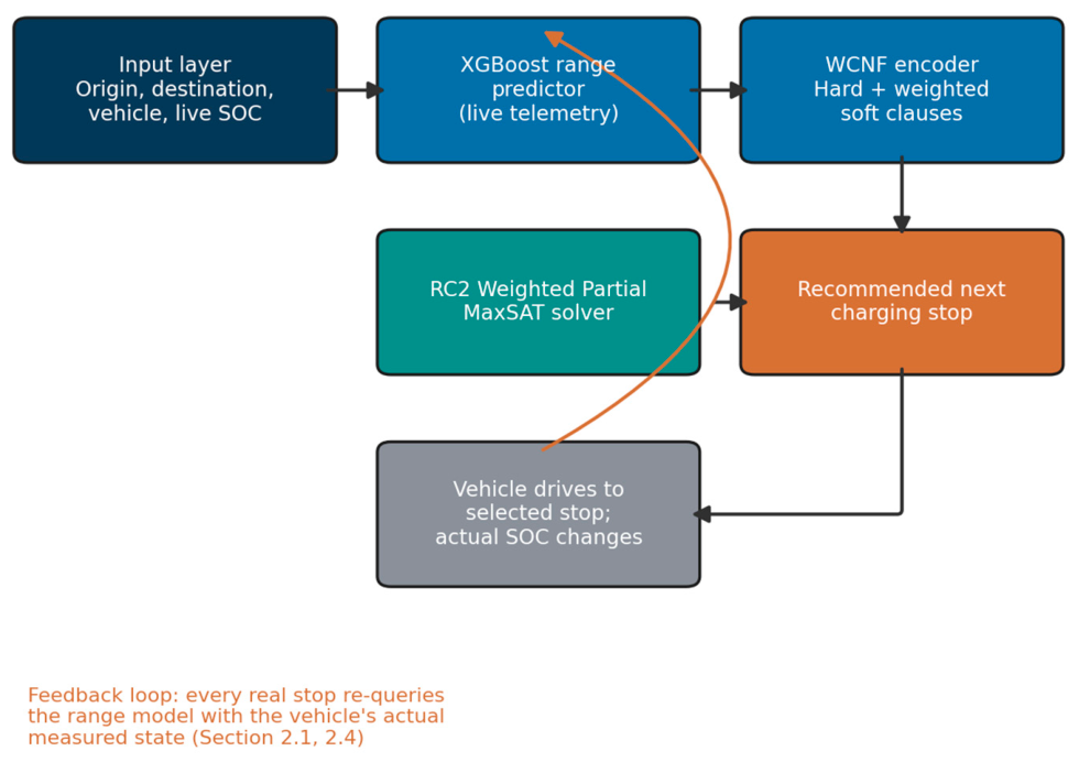
Figure 1.
RMSE and MAE (bars, left axis) and R² (line, right axis) for the four range-prediction candidates on the held-out test split.
Figure 1.
RMSE and MAE (bars, left axis) and R² (line, right axis) for the four range-prediction candidates on the held-out test split.
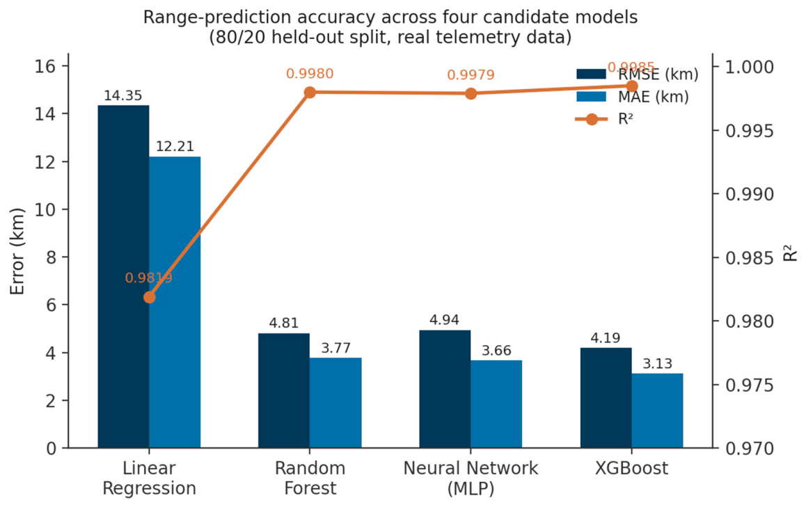
Figure 2.
Average total trip time across the five benchmark trips for the proposed system and the two baselines.
Figure 2.
Average total trip time across the five benchmark trips for the proposed system and the two baselines.
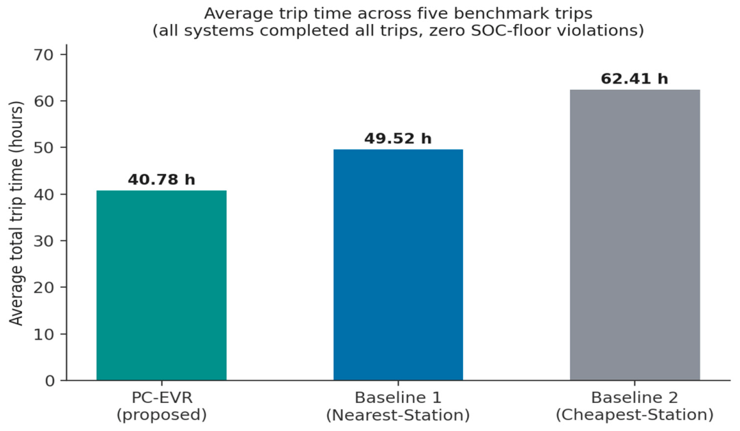
Figure 4.
Routes selected for the Pune–Hyderabad illustrative trip: (a) proposed system (two DC stops), (b) Baseline 1/Nearest-Station, and (c) Baseline 2/Cheapest-Station (AC-only stops, one below the 20% SOC floor). Screenshots captured from the deployed Streamlit application.
Figure 4.
Routes selected for the Pune–Hyderabad illustrative trip: (a) proposed system (two DC stops), (b) Baseline 1/Nearest-Station, and (c) Baseline 2/Cheapest-Station (AC-only stops, one below the 20% SOC floor). Screenshots captured from the deployed Streamlit application.
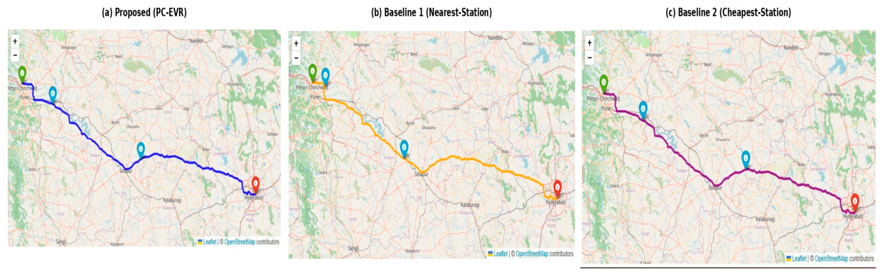

Table 1.
Weighted soft-clause objective: components, weights and rationale.
| Component | Weight | What It Captures |
| detour_km | 0.40 | Extra kilometres versus driving straight through (triangle-inequality detour) |
| progress_km | 0.20 | Reduction in remaining distance to the destination achieved by the candidate stop |
| time_penalty | 0.20 | Traffic-adjusted drive time plus a charger-power and connector-type penalty |
| cost_kwh | 0.12 | Modelled charging cost a tiebreaker rather than a primary driver |
| (1 − margin) | 0.08 | Residual safety-margin penalty, nudging toward a comfortable rather than minimal arrival SOC |
Table 2.
Urgency-scaled minimum-progress thresholds, shared by all three systems.
| SOC Remaining | Minimum Progress Required to Accept a Candidate |
| > 50% | 55% (only a station clearing most of the remaining distance) |
| 35–50% | 30% |
| 25–35% | 15% |
| < 25% | 5% (approaching the floor, take what is reachable) |
Table 3.
Representative sample of the vehicle specification table (8 of 30 verified Indian EV models).
Table 3.
Representative sample of the vehicle specification table (8 of 30 verified Indian EV models).
| Model | Battery (kWh) | Rated Range (km) | Charging Type |
| MG Comet EV | 17.3 | 230 | AC Type-2 |
| Tata Tiago EV | 24 | 285 | AC Type-2, DC CCS2 |
| Tata Nexon EV | 45 | 489 | AC Type-2, DC CCS2 |
| Hyundai Creta Electric | 51.4 | 510 | AC Type-2, DC CCS2 |
| Kia EV6 | 84 | 663 | AC Type-2, DC CCS2 |
| BYD Seal | 82.56 | 650 | AC Type-2, DC CCS2 |
| Mahindra BE 6 | 79 | 683 | AC Type-2, DC CCS2 |
| Mercedes-Benz EQS 580 | 107.8 | 857 | AC Type-2, DC CCS2 |
¹ The full 30-model table is provided as Supplementary Table S1.
Table 4.
The five fixed benchmark trips used for all system-level comparisons.
| Trip | Route | Vehicle | Starting SOC |
| T1 (short) | New Delhi → Agra | Tata Tiago EV | 70% |
| T2 (medium) | New Delhi → Jaipur | MG Comet EV | 60% |
| T3 (long, small battery) | New Delhi → Nagpur | Vayve Mobility Eva | 90% |
| T4 (long, large battery) | New Delhi → Chennai | Hyundai Ioniq 5 | 90% |
| T5 (very long) | New Delhi → Hyderabad | Kia EV6 | 85% |
Table 5.
Range-prediction accuracy comparison on the held-out test split (real telemetry data only).
Table 5.
Range-prediction accuracy comparison on the held-out test split (real telemetry data only).
| Model | RMSE (km) | MAE (km) | R² |
| Linear Regression | 14.347 | 12.211 | 0.9819 |
| Random Forest | 4.814 | 3.772 | 0.9980 |
| Neural Network (MLP) | 4.940 | 3.663 | 0.9979 |
| XGBoost | 4.193 | 3.129 | 0.9985 |
Table 6.
System-level benchmark: average trip time across the five trips of Table 4. ¹.
Table 6.
System-level benchmark: average trip time across the five trips of Table 4. ¹.
| System | Range Model | Selection Strategy | Avg. Trip Time (h) |
| PC-EVR (proposed) | XGBoost (live telemetry) | Weighted Partial MaxSAT | 40.78 |
| Baseline 1 (nearest) | OEM linear formula | Greedy: nearest station | 49.52 |
| Baseline 2 (cheapest) | Physics-informed static heuristic | Greedy: cheapest station | 62.41 |
¹ All three systems completed all five trips with zero SOC-floor violations.
Table 7.
Qualitative positioning of PC-EVR relative to manual planning and a 2026 commercial EV trip planner.
Table 7.
Qualitative positioning of PC-EVR relative to manual planning and a 2026 commercial EV trip planner.
| Capability | Manual / Human Planning | Google Maps EV Planner (2026) | PC-EVR (This Work) |
| Range estimate source | Mental estimate from rated range | Proprietary, unpublished model | XGBoost, trained & benchmarked (RMSE ≈ 4.2 km) |
| Whole-trip re-solving | One decision at a time | Yes, on supported routes | Yes, re-solved at every decision point |
| Safety constraint | Driver judgement only | Not published / not verifiable | 20% SOC floor, hard solver constraint |
| India-specific national-scale validation | Only the driver's own vehicle | Not confirmed for Indian models | 30 Indian EV models, 39,641-station registry |
| Published, auditable method | N/A | Closed commercial system | Fully documented and reproducible |
Table 8.
Outcome summary for the Pune–Hyderabad illustrative trip, run independently of the Table 4 benchmark set.
Table 8.
Outcome summary for the Pune–Hyderabad illustrative trip, run independently of the Table 4 benchmark set.
| System | Distance (km) | Stops | Cost (₹) | Energy (kWh) | Pred. Initial Range (km) | Trip Time (h) | SOC at Dest. (%) | SOC-Floor Breach |
| Proposed (PC-EVR) | 587.37 | 2 | 383.55 | 54.05 | 152.5 | 10.61 | 33.5 | None |
| Baseline 1 (Nearest) | 602.00 | 2 | 394.68 | 55.40 | 195.6 | 21.14 | 22.2 | None |
| Baseline 2 (Cheapest) | 589.96 | 2 | 338.57 | 54.29 | 192.2 | 29.10 | 44.7 | Yes (19.1%, 0.9 pts under floor) |
Table 9.
Charging-stop detail for the Pune–Hyderabad illustrative trip, all three systems.
| System | Station | City | Type | Power (kW) | Cost (₹/kWh) | Dist. from Origin (km) | SOC on Arrival (%) | SOC After Charge (%) | Charging Time (min) |
| Proposed | BPCL – Warwand | Warwand | DC | 60 | 7.5 | 86.15 | 22.4 | 90 | 31.7 |
| Proposed | HPCL – Solapur | Solapur | DC | 30 | 7.5 | 311.22 | 44.0 | 90 | 43.9 |
| Baseline 1 | UJOY – Pune | Pune | AC | 3.3 | 10 | 30.65 | 33.7 | 95 | 501.3 |
| Baseline 1 | IOCL – Solapur | Solapur | AC | 3.3 | 6 | 246.12 | 50.9 | 95 | 360.5 |
| Baseline 2 | IOCL – Pune | Pune | AC | 3.3 | 6 | 102.28 | 19.1 | 95 | 621.1 |
| Baseline 2 | IOCL – Osmanabad | Osmanabad | AC | 3.3 | 6 | 344.23 | 45.5 | 95 | 404.8 |
The IOCL – Pune stop (Baseline 2) arrived at 19.1% state of charge, 0.9 percentage points under the 20% hard floor of Section 2.2; this is a property of this single trip's routing corridor and station availability, and does not alter the zero-violation result reported for the separate, fixed five-trip benchmark of Table 6.
Disclaimer/Publisher’s Note: The statements, opinions and data contained in all publications are solely those of the individual author(s) and contributor(s) and not of MDPI and/or the editor(s). MDPI and/or the editor(s) disclaim responsibility for any injury to people or property resulting from any ideas, methods, instructions or products referred to in the content. |
© 2026 by the authors. Licensee MDPI, Basel, Switzerland. This article is an open access article distributed under the terms and conditions of the Creative Commons Attribution (CC BY) license (http://creativecommons.org/licenses/by/4.0/).
Copyright: This open access article is published under a Creative Commons CC BY 4.0 license, which permit the free download, distribution, and reuse, provided that the author and preprint are cited in any reuse.