

Submitted:
18 September 2026
Posted:
20 September 2026
You are already at the latest version
Abstract
The increase in the reliability and safety levels of electrical power devices plays a key role in the transition toward aviation electrification. Safety-critical equipment, such as propulsion motors, must comply with stringent requirements to obtain airworthiness certification. Permanent Magnet Synchronous Motors (PMSMs) have emerged as a suitable technological solution for high-performance flight control actuation systems, and their extension to propulsive functions appears promising. Nevertheless, the reliability of PMSM power electronics converters is still far from the levels required by certification; therefore, motors must incorporate fault-tolerant capabilities in order to be considered flightworthy. In this context, the development of prompt and effective Fault Detection and Isolation (FDI) algorithms is essential. This paper presents the Model-in-the-Loop (MIL) validation of a Neural Network (NN) algorithm for the detection and isolation of MOSFET faults and open-phase faults in PMSM power drives. The approach is based on a feedforward NN trained on simulation-generated data for a multi-class classification problem, combined with a counter-based decision logic to ensure fast, robust, and computationally efficient operation. A feature selection analysis is also carried out to reduce the network size without significant degradation in the classification accuracy. For the MIL validation, the NN-based algorithm is integrated within a high-fidelity dynamic model of an electrically driven UAV propeller, including the simulation of the three-phase PMSM with Field-Oriented Control (FOC) of the motor currents, digital signal processing, together with a model of the aerodynamic loads derived from Blade Element Momentum Theory (BEMT). Faults are injected at different operating speeds and under uncertain environmental conditions, to evaluate the FDI performance in terms of detection latency, isolation capability, and robustness. The results demonstrate the effectiveness of the approach, which, owing to its straightforward generalization, can be extended to other fault categories and leveraged to support the development of PMSMs with fault-tolerant control capabilities.
Keywords:
PMSM drive
; MOSFET fault
; open-circuit fault
; fault detection and isolation
; FDI algorithm
; neural network
; model in the loop validation
1. Introduction
The increasing use of electrical devices in aviation, driven by decarbonization policies [1,2] and performance enhancements in terms of energy efficiency [3] and fuel consumption reduction in hybrid electric propulsion [4,5] has raised growing concerns about the reliability of onboard electrical systems [6,7]. All onboard electronics of an aircraft must comply with specific standards, such as DO-254 [8]. Particularly, electric machines and power electronics should incur no more than one failure per one billion operating hours [9]. Permanent magnet synchronous motors (PMSMs) have emerged as a suitable technological solution in this context, owing to their light and compact design, high torque density, efficiency and scalability [10,11]. While PMSMs are already established for high-performance flight control actuation systems [12,13], where redundancy typically mitigates the impact of a single failure, their extension to propulsive functions [14,15,16] raises reliability stakes significantly, since a fault directly affects flight safety and cannot always rely on the same level of redundancy. PMSM drives experience several fault mechanisms, ranging from mechanical to electrical failures. Such faults can be grouped into three main categories: 1) machine faults, including stator and rotor failures; 2) power converter faults; 3) sensor faults [17]. Prior studies have indicated stator winding faults as the predominant failure mode in PMSMs [18,19], with statistical analysis indicating stator windings and power electronic switches as responsible for 50% to 70% of PMSM faults [20]. Such faults cause torque ripple and degradation of performance, making conventional control techniques no longer adequate. In addition, if they are not detected and accommodated in time, they can evolve into more serious faults. For these reasons, fault detection and isolation (FDI) algorithms are necessary to support fault-tolerant control. Existing FDI methods are usually classified into three categories: model-based, signal-based, and data-driven methods. Model-based methods compare measurements with model-based observations, but they suffer from model uncertainties [21]. Signal-based methods analyze relevant signal changes in the time or frequency domain, such as in fast Fourier transform (FFT) [22,23], but they either require long measurement times [24] or rely on domain expertise [25]. Data-driven approaches have recently gained attention given their ability to learn fault patterns directly from measured signals without explicit system modeling and with generalization capability. In this regard, for example, recent advancements focus on the transfer learning (TL) technique, consisting of the full extraction of universal fault symptoms applicable to various diagnostic tasks [26,27], with Skowron and Krzysztofiak [28] training a deep convolutional neural network (CNN) on a mathematical model of a PMSM before testing it on real hardware. In [18], SE-ResCNN is proposed for real-time diagnosis of stator windings faults in PMSM, obtaining an average diagnostic accuracy of more than 98% on experimental results of a PMSM drive platform. In [29] Zhang et al. propose a one-dimensional CNN for open-circuit faults in inverter IGBTs, reaching 99.84% detection accuracy within a sample length of 10.24 ms. Geng et al. [30] developed a digital twin framework for PMSMs that generates simulated fault datasets and employs a CNN-based architecture for fault classification and onset detection, reporting 98.08% accuracy on the validation set and 10-20 ms onset detection latency. Despite these advances in data-driven method applications, the computational complexity of deep learning architectures may exceed the onboard processing capabilities available on aircraft systems. Additionally, existing works rarely address the regulatory dimension: the latest EASA guidelines on AI integration in aerospace systems [31] explicitly recommend real-time monitoring of the output of the AI/ML constituent, a requirement that is seldom incorporated into the design of FDI algorithms. Finally, most studies validate their approaches under idealized or laboratory conditions, without assessing robustness under uncertain operating environments representative of real flight scenarios. This paper addresses these gaps (namely, computational footprint, validation realism, and regulatory compliance) by presenting the Model-in-the-Loop (MIL) validation of a Neural Network (NN)-based FDI algorithm for MOSFET and open-phase faults in PMSM power drives, designed specifically for aerospace propulsion applications. The proposed approach combines a compact feedforward NN, whose limited size keeps computational demand compatible with onboard processing constraints, with a counter-based decision logic that enforces robustness against misclassifications while ensuring compliance with EASA real-time monitoring guidelines. A feature selection analysis is conducted to minimize computational footprint without significant loss in classification accuracy. The workflow was previously proposed in [32], where it was validated under idealized sensing conditions. The present work expands this study by introducing realistic sensor noise, propeller aerodynamic loads derived from Blade Element Momentum Theory (BEMT), and by validating the algorithm’s robustness through a Monte Carlo analysis on key motor parameters. The algorithm is trained and tested on simulation-generated data and validated through MIL within a high-fidelity dynamic model of the full electrical propulsion system, integrating a three-phase speed-controlled PMSM with Field-Oriented Control (FOC) and digital signal processing, enabling fault injections under realistic aerodynamic operating conditions. Results demonstrate effective fault isolation with detection latencies ranging from 6 to 14 ms and increasing to 20 ms for the most challenging fault classes under combined parametric and timing perturbations. The proposed algorithm shows robustness against parametric uncertainties, and its design philosophy facilitates extension to other fault categories and integration with fault-tolerant control strategies.
2. Materials and Methods
A scheme of the reference UAV PMSM drive is reported in Figure 1.
The system includes:
- the Flight Control Computer (FCC), providing the motor speed setpoint (ωmdem);
- the speed controller, generating the quadrature current demand in the d-q axis reference frame (Iqdem) for the current controller;
- the current controller, which regulates the direct and quadrature axis currents through high-bandwidth proportional-integral controllers with anti-windup compensation. According to the Field-Oriented Control (FOC) strategy, the d-axis current is regulated to zero, while the q-axis current controls electromagnetic torque generation. Feedforward compensation of the speed-dependent cross-coupling terms is implemented to decouple the d and q-axis current dynamics. Dynamic voltage saturation limits the commanded voltage vector according to the available DC-link voltage. The controller generates the voltage references Vd and Vq;
- the inverse Clarke-Park transformation, which converts Vd and Vq into the three-phase voltage references Va, Vb and Vc;
- the space-vector pulse-width modulation (SVPWM) stage, which computes the duty cycles required to synthesize the commanded stator voltage vector;
- the three-phase voltage-source inverter, consisting of three switching legs composed of six MOSFETs, supplied by an ideal DC voltage source, VDC, as shown in Figure 3;
- the sensors and digital signal-processing subsystem, including phase current sensors and a motor-shaft angular-position sensor, modeled using their datasheet bandwidths. The measured signals are processed through an analogue-to-digital acquisition chain including additive white Gaussian noise, zero-order hold sampling, finite full-scale range and resolution, and quantization. All digital processing associated with the control laws and feedback acquisition is performed at a sampling frequency of 10 kHz;
- the direct Clarke-Park transformation, which converts the measured phase currents Ia, Ib and Ic into the synchronous-frame feedback Id fb and Iq fb used by the current control loop;
- the discrete differentiation and filtering of the measured motor position to compute the motor speed feedback ωm fb;
- a three-phase PMSM in wye-wound configuration with constant permanent magnet flux linkage, d-q axis inductances Ld and Lq , and phase inductance L and resistance R. The PMSM model was experimentally validated in [33];
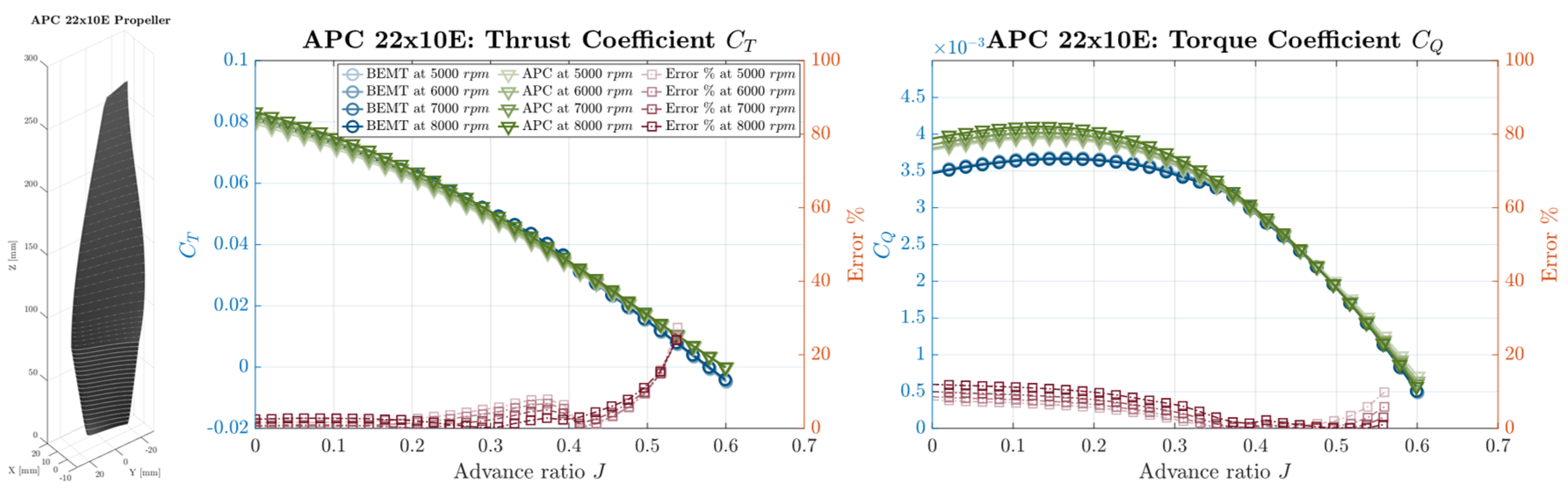
- an APC 22x10E propeller, rigidly coupled with the motor shaft. Its aerodynamic performance was imported into the model through the two-dimensional maps of thrust CT (J, ω) and torque CQ (J, ω) coefficients, expressed as a function of the advance ratio J and the rotational speed ω. These maps were generated using the BEMT-based method described in [34]. The resulting maps are shown in Figure 2 for selected rotational speeds, together with a comparison against the APC manufacturer data.
Figure 2.
APC 2210E propeller: reconstructed blade geometry (left); comparison between the BEMT predictions and the manufacturer-provided APC data for the thrust coefficient (centre) and torque coefficient (right) at selected rotational speeds.
Figure 2.
APC 2210E propeller: reconstructed blade geometry (left); comparison between the BEMT predictions and the manufacturer-provided APC data for the thrust coefficient (centre) and torque coefficient (right) at selected rotational speeds.
The simulator is developed in MATLAB/Simulink using Simscape libraries for modelling the electrical machine and the power electronics. It enables direct fault injection into the inverter MOSFETs, thereby defining 10 operating conditions (Figure 3): one nominal condition, six open-switch fault conditions, corresponding to the high-side and low-side MOSFETs of each inverter leg, and three open-phase fault condition, one for each stator phase. Operation class labeling is presented in Table 1.
Figure 3.
Inverter open-phase power switches faults: Case 1, a single phase low MOSFET is faulted; Case 2, a single phase high MOSFET is faulted; Case 3, both MOSFETs of a phase are faulted.
Figure 3.
Inverter open-phase power switches faults: Case 1, a single phase low MOSFET is faulted; Case 2, a single phase high MOSFET is faulted; Case 3, both MOSFETs of a phase are faulted.
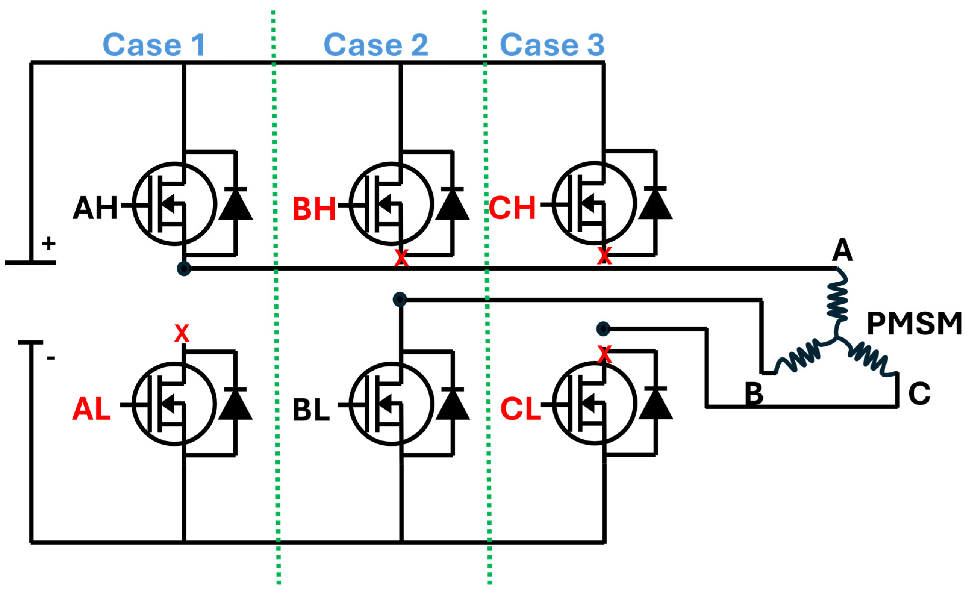
Figure 4 illustrates the workflow for the design and implementation of the algorithm. First, a dataset for training the neural network was generated in Simulink. Then, the NN structure was defined, and a feature selection analysis was conducted in MATLAB to define the final NN architecture. Subsequently, the selected NN was implemented in Simulink for online inference and testing of the algorithm during simulation. Finally, a robustness analysis of the algorithm was conducted by varying some key model parameters. The fault dataset was generated using the simulator according to the parameters listed in Table 2. For each simulation run, the model was initialized for cruise condition at the chosen reference speed. Particularly, during each simulation, the following time-series measurements were collected, as well as the instantaneous operating condition: ωmdem, ωmfb, Ia, Ib, Ic, Iqdem, Iqfb, Idfb, Iα, Iβ. As a result of the injection of each fault at exactly half of total simulation time, the generated dataset is inherently imbalanced with nominal-condition subset being nine times larger than faulty subsets. This was a design choice to reflect realistic operating conditions and data acquisition where systems predominantly operate in a healthy mode.
After dataset generation, the following data preprocessing steps were applied:
- Fixed-window averaging, with the window length empirically selected to correspond approximately to half an electrical period under the considered operating conditions (10 samples at the 10 kHz sampling rate used for data acquisition, given that successive positive current peaks are separated by approximately 20 samples);
- Division of the dataset into training and test subsets, with the data collected at intermediate reference speeds, 6300 rpm and 6400 rpm, reserved for testing to evaluate the NN’s interpolation capability within the trained speed range;
- Z-score normalization;
- Random shuffling of the subsets.
The window length was selected empirically by comparing the classification performance obtained with 10- and 20-sample windows, corresponding to half and one full electrical period, respectively. The shorter window achieved slightly higher validation accuracy while also halving the acquisition time required to compute each input sample, thereby reducing overall detection latency. It was therefore adopted for the remainder of the study. Fixed-window averaging was adopted to train the NN on representative time-averaged signals rather than on instantaneous samples, which may be strongly affected by the periodic behavior of the electrical variables. Relying solely on instantaneous current samples may not provide sufficient discriminatory information, as identical current values can occur at different points of the electrical cycle under both healthy and faulty operating conditions. Averaging over a fixed window reduces the influence of the instantaneous acquisition of the signal while preserving the fault-related features for classification, leading to a more robust detection process. The detection task is addressed as a multi-class classification problem, with a maximum of ten input features and ten output classes as reported in Table 1.
Figure 5 illustrates the NN architecture; training hyperparameters are listed in Table 3. The number of hidden neurons was selected empirically through a sensitivity analysis, training and evaluating networks with 10, 20, 50, 75, 100, 150, and 200 hidden neurons on the same train/validation/test split.
After offline training and validation in MATLAB using the Deep Learning Toolbox, the resulting network was exported and embedded into the Simulink MIL model using a Predict block, enabling online inference during simulation. For fault isolation, the NN prediction output is evaluated by a state machine whose block diagram is shown in Figure 6.
The isolation algorithm is implemented as a state machine in the Stateflow environment. It takes as input the class predicted by the NN. If no fault condition is detected, it remains in the Nominal state. When a fault is detected, it enters its corresponding fault state and starts updating a counter. If the subsequent NN prediction matches the current fault state, the counter increases by two; if it is different, it decreases by one. If the counter becomes negative, the state returns to Nominal and the counter is reset. When the counter exceeds a threshold value of 4, the isolation algorithm latches the corresponding fault state, finalizing the isolation. The threshold value is selected for a practical trade-off between robustness and detection speed. A lower threshold would increase sensitivity to misclassification but improve speed, while a higher one would increase robustness but decrease responsiveness. The algorithm was tested on the simulator according to simulation parameters listed in Table 4. In particular, the fault-injection time was randomized.
Finally, to characterize the robustness of the FDI performance, a full-factorial analysis based on Monte Carlo sampling was performed on two parameters: the phase resistance R and the phase inductance L. Other electromechanical and mechanical parameters, such as motor torque constant ktd, were not varied because the mechanical dynamics intuitively evolve on a substantially slower time scale than the electrical transients associated with the considered faults. For each parameter, N = 50 samples were drawn from a normal distribution centered at the nominal value, with a standard deviation equal to 15% of the corresponding nominal value:
subject to the constraints:
i.e. each candidate was drawn repeatedly until it was both strictly positive and distinct from every previously accepted sample for that parameter. This produced two sampled sets:
The explored parameter space is the Cartesian product of the two sampled sets:
so that each simulation corresponds to a couple:
Each of the N2 = 2500 distinct parameter combinations was used to execute an independent simulation run while testing of all nine fault conditions, allowing the robustness of the proposed FDI algorithm to be assessed against simultaneous variation of the fundamental motor parameters. The number of samples was selected as a compromise between statistical representativeness and computational cost. Since the electrical propulsion system is modeled using a high-fidelity simulation environment that includes both the electrical drive and the propeller aerodynamic model, each simulation run entails a non-negligible computational burden. Consequently, increasing the number of samples would have led to a substantial increase in the overall execution time without providing a proportional improvement in the statistical significance of the robustness assessment. Additionally, to speed up simulations, the simulator settings have been modified as reported in Table 5. The increase in the simulation time step also contributes to test the FDI algorithm robustness as it effectively creates signals that differ from those used for training the NN. Additionally, speed step demand was included to perturb the system into a transient operation.
3. Results and Discussion
3.1. Hidden Layer Size Sensitivity Analysis
Figure 7 reports the train, validation, and test accuracy obtained for hidden layer sizes ranging from 10 to 200 neurons. This analysis was conducted to determine how far the hidden layer size could be reduced without compromising accuracy, with the aim of improving computational efficiency. Regarding the input size, the full feature input was considered for this analysis. The hidden-layer size yielding the highest test accuracy is indicated by a vertical dotted line. Class-wise test accuracies for the three open-phase fault classes (OA, OB, OC) are reported in Table 6. These were consistently identified as the most challenging classes to classify and therefore used to guide the selection of number of hidden layer neurons.
3.2. Feature Selection Analysis
Figure 8 presents the results of the feature analysis. Various combinations of signals were tested, although not all permutations were evaluated. Particular emphasis was placed to current subsets, including combinations of phase currents, d-q axis currents, and alpha-beta currents. For example, in rows 15, 16, 22, three redundant configurations were tested: (Ia, Iα, Iβ), (Ib, Iα, Iβ), (Ic, Iα, Iβ). From an algebraic standpoint, these three subsets are formally equivalent and, under the isolated-neutral assumption (Ia + Ib + Ic = 0), equivalent to (Iα, Iβ). Nevertheless, testing the three variants serves both in verifying the insensitivity of the classifier to specific phase currents retained and in confirming the above assumption.
3.3. FDI Algorithm Testing with Random Fault Injection
Figure 9 and Figure 10 present the algorithm testing results according to parameters listed in Table 4. In Figure 9, the three faults of the motor phase A are presented. The measured phase current is shown in the first row. The second row contains the PMSM condition state (Table 1): the actual one and the state predicted by the algorithm. When a fault is isolated, the corresponding state is latched. Finally, the associated counter is presented in the last row. Figure 10 includes the confusion matrices for all the test runs. To evaluate the performance of the NN classifier, four standard metrics were considered: True Positive Rate (TPR), False Negative Rate (FNR), Precision, and the F1-score. These metrics are computed from the number of true positives (TP), true negatives (TN), false positives (FP), and false negatives (FN) computed over the test dataset. True positive rate, also referred to as recall or sensitivity, measures the proportion of actual positive instances that are correctly identified:
The false negative rate measures the complementary metric to the TPR, and it measures the proportion of actual positive instances that are incorrectly classified as negative:
Precision (P) quantifies the proportion of instances predicted as positive that are indeed positive, thereby reflecting the reliability of positive predictions:
Finally, the F1-score combines P and TPR into a single metric via their harmonic mean, providing a balanced measure that accounts for both false positives and false negatives:
The metric F1 is particularly informative in the presence of class imbalance, because accuracy may provide a misleading assessment of classifier performance. A high F1-score indicates that the model produces few false positives relative to its predicted positives (high P) and few false negatives relative to the total of actual positives (high TPR). Since the fault-diagnosis problem is formulated as a multi-class problem, the four metrics were computed using a one-vs-rest strategy. For each class, the corresponding row and column of the confusion matrices were used to define the metrics treating the considered class as positive and the remaining as negatives.
3.4. Uncertainty Quantification via MONTE Carlo Analysis
Figure 11 shows the parameter distributions generated for the Monte Carlo analysis. Each subplot shows the normalised histogram of the N = 50 drawn samples grouped into bins, the kernel density estimate (KDE) of the empirical distribution, and the theoretical target Gaussian PDF. Dashed vertical lines mark the nominal parameters values. Shaded pink regions indicate the ±1σ and ±2σ intervals of the theoretical distribution. The empirical mean and standard deviation are reported for comparison with their theoretical values in the annotation box.
Figure 12 reports the distributions of TPR, Precision, and F1-score. Box plots are used, with the mean of each metric overlaid as a horizontal segment. The interquartile ranges quantify the variability of the metrics under the combined variation of the two parameters.
Figure 13 and Figure 14 include the confusion matrices obtained from the Monte Carlo MIL simulation. The results are averaged over the 2500 runs, and they provide a class-by-class characterization of the classifier behaviour across the explored parameter space.
Figure 15 shows scatter plots of the TPR, Precision, and F1-score. For each sampled parameter value, the mean across the 50 combinations with the drawn values of the other parameter is presented.
Figure 16 shows the isolation success rate, together with fault isolation time distribution.
Figure 17 presents the mean isolation time against parameters variation.
Figure 18 presents the best and worst 5% Monte Carlo runs in terms of F1-score as function of the motor parameters.
3.5. Discussion of Results
In Figure 7, classification accuracy increases sharply between 10 and 25 neurons, from approximately 86% to above 94%, and then improves gradually, reaching local maxima at 75 and 150 neurons (approximately 96%). A plateau is evident, suggesting that further increases in hidden layer size provide limited benefits for the available training data. Based on the results reported in Table 6, a hidden layer size of 75 neurons was selected as the configuration offering the best trade-off between overall classification accuracy, performance on the most challenging fault classes, and network size.
In Figure 8, all six best-performing subsets either include the full set of features or exclude less informative signals. This suggests that the classifier is robust to the removal of minor features when core signals are retained, and that the network can learn discriminative fault patterns directly from the data without explicitly embedding the underlying physical relationships among the signals. A noticeable drop occurs in row 7 (92.39%) when Iqdem is removed. The drop becomes more pronounced from rows 8 to 10, where the additional removal of other features further reduces the accuracy. In rows 11–14, a further accuracy drop is observed due to the combined removal of either d-q current signals or α-β current signals together with phase currents. The lower-performing subsets, with accuracies around 72%, correspond to rows 15–23. The subsets retain either a few features or none of the commanded inputs, and the accuracy drops significantly, suggesting that the classifier cannot discriminate between fault classes with insufficient observability. The worst-performing subsets correspond to rows 24 and 25, with accuracies around 58%. Here, the d-q current signals are insufficient to discriminate between the different classes, and the addition of speed signals does not provide adequate discriminative information because the retained signals exhibit similar responses across multiple fault classes. The configuration of row 1 was selected for the remainder of the study and integrated into the complete FDI algorithm because it provided the highest validation accuracy while using only six features.
In Figure 9, the single AH MOSFET fault has the shortest isolation time, with 6 ms between the random fault-injection time and the counter crossing the threshold and latching the new fault state. Before the fault state is latched, the counter decreases from 4 to 3, implying a temporary misclassification by the NN. Nevertheless, the overall FDI algorithm still achieves correct isolation. The single AL MOSFET fault and the phase-A open-circuit fault both exhibit two counter decrements during the initial detection transient. However, the FDI algorithm recovers and isolates the correct fault in approximately 11 ms in both cases.
In Figure 10, the Nominal condition shows a 100% TPR, meaning that this condition is never misclassified as a faulty one and that sensor noise does not induce false alarms during healthy operation. Single MOSFET fault classes achieve a TPR in the range of 63.7–71.9%, with most misclassifications assigned to the Nominal class (8.8 to 30.3%) and toward open-phase faults. Open-phase fault classes show the lowest accuracy, with TPR in 36.2–44.4% range. These classes show substantial confusion with both the Nominal condition and the single MOSFET fault of the same phase: class 8 is misclassified as class 1 in 25.6% of cases, class 9 as class 3 in 20.3% of cases, and class 10 as class 5 in 17.2% of cases. Overall, these results indicate that sensor noise disproportionately affects the fault classes that already exhibit the lowest accuracy under ideal sensing conditions considered in [32], where single MOSFET faults had a TPR in the range of 96.1–98.1%, while open-phase faults in the range of 86.1–92.1%. This pattern indicates that open-phase faults, involving simultaneous loss of both low- and high-side switches on a phase, produce less distinguishable current signatures than single-switch faults, making them harder to isolate quickly. However, the isolation on all the nine faults still achieves 100%, meaning that the algorithm can compensate for misclassification from the NN.
Figure 11 shows the normalized histograms of the two parameters sampled in the Monte Carlo analysis (Eq. 4) compared with their theoretical Gaussian probability density functions (PDF). For both phase resistance and inductance, the empirical mean and standard deviation closely match the theoretical values. For phase resistance, the empirical mean and standard deviation differ from their theoretical values by −3.04% and −8.27%, respectively; for phase inductance, the corresponding deviations are +3.48% and −2.80%. While the phase inductance KDE curve closely tracks the theoretical Gaussian PDF, the phase resistance KDE shows a larger deviation, but still most samples fall within the ±2σ band, as expected for a Gaussian distribution. Visible discrepancies between the empirical and theoretical distributions are a consequence of the finite sample size and are statistically expected. Nevertheless, the drawn outcome still appears to be satisfactory for the purpose of the study, given the necessary trade-off between sample size and computational burden for the Monte Carlo analysis.
Figure 12 shows the sensitivity of TPR, Precision and F1-score to the combined variations in the parameters defined in the Equation 4, as well as the modified simulation time step (Table 5). The six single-MOSFET fault classes exhibit higher TPR values than the open-phase faults, with range of 80–90% compared with 75–80%. The TPR of the Nominal condition presents the most elongated boxplot, indicating that appreciable variability characterizes the detection of this condition under parameter uncertainty. For Precision, all faulty conditions have mean values close to 90%, while for the Nominal condition it drops to 55%. As a consequence, the Nominal-condition F1-score is the lowest, with faulty conditions well above 80%. The discrepancies in the three metrics between the single simulation run with nominal parameters (Figure 10) and the Monte Carlo analysis can be primarily attributed to the parameters used for simulation. The single test had a simulation duration of 0.05 s with the fault randomly injected between 10 and 20% of the total duration. For the uncertainty analysis, by contrast, the fault was always injected at one tenth of the total simulation duration, therefore removing the class imbalance since all classes now contained almost the same number of instances along a run. This behaviour can also be inferred from the confusion matrices shown in Figure 13 and Figure 14. Moreover, it can be observed that the average misclassification rate decreases with respect to the single test run.
Figure 15 shows that the metrics respond differently to the two Monte Carlo parameters. Phase resistance exhibits a V-shaped trend across all three metrics, with a minimum slightly shifted to the left of the nominal value; the highest values are found at the extremes of the sample range, although the overall variation remains limited, reaching a maximum deviation of about 3%. Phase inductance, in contrast, shows a markedly higher sensitivity, with all three metrics varying by approximately 15% across the sampled range and consistently increasing with L.
The algorithm can achieve 100% isolation success rate across the entire explored parameter space, with isolation latency comparable with values reported in literature. Figure 16 confirms that the NN detects more precisely the single MOSFET fault classes; in fact, they present the shortest and most consistent isolation times, with medians ranging from approximately 8 ms to 11 ms, and interquartile ranges generally within 5-12 ms. Whiskers on OAL and OBH shows wider dispersion, extending up to 20 ms.
In Figure 17, the trends appear mirrored with respect to those of Figure 15. Specifically, phase resistance shows the longest fault isolation times at the parameter values corresponding to the vertex of the V-shaped trend observed for TPR, Precision and F1-score. The same inverse relationship holds for phase inductance, where isolation time is longer where classification metrics were lowest.
Figure 18 confirms and visually summarizes the trends already discussed for Figure 15 and Figure 17. The worst performing 5% of Monte Carlo runs (blue) cluster predominantly at lower phase inductance values. Conversely, the best performing 5% runs (red) are concentrated at higher values of phase inductance, forming a clearly separated cluster in the parameter space. The clear separation of the two clusters indicates that classification performance is primarily driven by phase inductance, consistent with the lower sensitivity to phase resistance already observed in Figure 15.
4. Conclusions and Future Perspectives
When compared to recent data-driven FDI approaches, the present classifier exhibits a validation accuracy (95.81%) that is broadly in line with, though slightly below, CNN-based architectures reported in the literature. This gap is consistent with the architecture adopted in this work: a single-hidden-layer feedforward network was selected over deeper convolutional architectures specifically to minimize computational footprint, at the expense of some raw classification accuracy. Notably, the isolation latency achieved under nominal conditions (6 to 12 ms) is comparable to the 10–20 ms onset detection reported in previous works. Furthermore, a systematic robustness assessment against combined parametric uncertainty was performed: while the present NN classifier alone shows a TPR degradation under 15% parameter perturbation, the counter-based isolation logic recovers full fault isolation capability (100% success rate) across the explored parameter space. This suggests that, although the standalone classification accuracy of a compact NN may not match deeper architectures trained and validated under idealized conditions, the overall FDI algorithm proposed here achieves comparable or superior practical robustness.
Some limitations of the present study should be acknowledged. First, validation was conducted exclusively in a Model-in-the-Loop environment; no Hardware-in-the-Loop (HIL) testing or experimental validation on a physical motor drive was performed, and the transition to embedded hardware may introduce additional sources of latency, noise, and quantization error not captured by the present simulation framework. Second, the Monte Carlo analysis still used a reduced number of samples (50), due to exponential increase of computational burden. Third, the robustness analysis was restricted to two motor parameters (phase resistance and phase inductance); other sources of uncertainty relevant to aerospace applications, such as temperature-dependent magnets flux-linkage variation or supply voltage fluctuations, were not explicitly modeled and are left for future investigation. Finally, the counter threshold value of four was selected heuristically as a practical trade-off between detection speed and robustness, rather than through a systematic sensitivity analysis; a dedicated optimization of this parameter could further improve the latency-robustness trade-off. These limitations do not undermine the validity of the presented results but delineate the scope of the current validation stage and motivate the next steps toward HIL and experimental testing.
These results support the feasibility of embedding computationally efficient neural network classifiers within safety-critical FDI pipelines for aerospace electric propulsion if the classification stage is paired with a robust decision logic capable of mitigating residual misclassification. The design philosophy adopted in this work, i.e., separating a real-time-compliant classifier from a dedicated isolation logic, facilitates extension to other fault categories beyond MOSFET and open-phase faults and provides a foundation for integration with fault-tolerant control strategies aimed at maintaining propulsive capability following a detected fault.
Author Contributions
Conceptualization, A.M. and G.D.R.; methodology, A.M. and G.D.R.; software, A.M. and M.L.; validation, A.M., G.D.R. and M.L.; formal analysis, A.M.; investigation, A.M.; resources, G.D.R; data curation, A.M.; writing—original draft preparation, A.M. and M.L.; writing—review and editing, A.M., G.D.R. and M.L.; visualization, A.M., G.D.R. and M.L.; supervision, G.D.R.; project administration, G.D.R.. All authors have read and agreed to the published version of the manuscript.
Funding
This research received no external funding.
Data Availability Statement
The original data presented in the study are available on Zenodo at https://doi.org/10.5281/zenodo.22744390.
Acknowledgments
The authors wish to thank Dr. Aleksander Suti for his early contribution to the development of the PMSM model, and Eng. Valerio Bonini and Eng. Eugenio Rovera for their support.
Conflicts of Interest
The authors declare no conflicts of interest.
Abbreviations
The following abbreviations are used in this manuscript:
| AI | Artificial intelligence |
| BEMT | Blade element momentum theory |
| CNN | Convolutional neural network |
| EASA | European Union aviation safety agency |
| FDI | Fault detection and isolation |
| FOC | Field oriented control |
| HIL | Hardware in the loop |
| KDE | Kernel density estimation |
| MIL | Model in the loop |
| N | Nominal – healthy condition |
| NN | Neural network |
| OAH | Open high side MOSFET phase A |
| OAL | Open low side MOSFET phase A |
| OBH | Open high side MOSFET phase B |
| OBL | Open low side MOSFET phase B |
| OCH | Open high side MOSFET phase C |
| OCL | Open low side MOSFET phase C |
| OA | Open-phase A |
| OB | Open-phase B |
| OC | Open-phase C |
| Probability density function | |
| PMSM | Permanent magnet synchronous motor |
| SVPWM | Space vector pulse width modulation |
| TL | Transfer learning |
References
- Clean Aviation EU. Available online: https://www.clean-aviation.eu/research-and-innovation/clean-aviation/our-energy-efficiency-and-emission-reduction (accessed on 10 December 2025).
- Jiang, C.; D’Alfonso, T.; Post, J. Aviation Decarbonization – Policies and Technologies to Support Decarbonization of the Aviation Sector. Transp. Res. D. Transp. Environ. 2024, 127, 104055. [Google Scholar] [CrossRef]
- Buvarp, D.; Leijon, J. Electric Aircraft: A Review of Challenges and Emerging Technologies. Discov. Appl. Sci. 2026, 8, 444. [Google Scholar] [CrossRef]
- Mazzone, A.; Suti, A.; Di Rito, G.; Mattei, G. Development of a Hybrid-Electric Propulsion System Simulator for a Lightweight Fixed-Wing UAV and Design of On-Board Power Management Strategies. Aerotec. Missili Spaz. 2026, 105, 579–601. [Google Scholar] [CrossRef]
- Hui, Y.; Li, H.; Chai, J.; Kang, Y. Research on Large Hybrid Electric Aircraft Based on Battery and Turbine-Electric. Energies 2024, 17, 5062. [Google Scholar] [CrossRef]
- Emmanouil, K. Reliability in the Era of Electrification in Aviation: A Systems Approach. Microelectron. Reliab. 2020, 114, 113945. [Google Scholar] [CrossRef]
- Keilmann, R.; Kösters, L.; Radomsky, L.; Franzki, J.; Henke, M.; Heere, M.; Mallwitz, R. A Comprehensive Review of Reliability Factors in All-Electric Aviation. CEAS Aeronaut. J. 2026, 17, 969–986. [Google Scholar] [CrossRef]
- Cano, T.C.; Castro, I.; Rodriguez, A.; Lamar, D.G.; Khalil, Y.F.; Albiol-Tendillo, L.; Kshirsagar, P. Future of Electrical Aircraft Energy Power Systems: An Architecture Review. IEEE Trans. Transp. Electrif. 2021, 7, 1915–1929. [Google Scholar] [CrossRef]
- Siadatan, A.; Kalantarikhalilabad, A.; Rezaei-Zare, A. Reliability and Fault-Tolerance Assessment of PMSM Drive for Electric Aircraft Applications. In Proceedings of the 2023 IEEE International Electric Machines & Drives Conference (IEMDC); IEEE, 15 May 2023; pp. 1–7. [Google Scholar]
- Shen, Q.; Zhou, Z.; Li, S.; Liao, X.; Wang, T.; He, X.; Zhang, J. Design and Analysis of the High-Speed Permanent Magnet Motors: A Review on the State of the Art. Machines 2022, 10, 549. [Google Scholar] [CrossRef]
- Bianchi, N.; Michieletto, D.; Cinti, L.; Conto, C.; Carlet, P.G.; Brunetti, M.; Nesci, A. Permanent Magnet Synchronous Motor Drives for More-Electric Aircraft. In Proceedings of the 2022 International Symposium on Power Electronics, Electrical Drives, Automation and Motion (SPEEDAM); IEEE, 22 June 2022; pp. 871–876. [Google Scholar]
- Zhang, K.; Chen, T.; Li, Z.; Wu, F.; Si, B. Robust Adaptive Position Control of PMSM Actuators for High-Speed Flight Vehicles Under Thermal Extremes. Electronics 2026, 15, 1742. [Google Scholar] [CrossRef]
- Lucarini, M.; Di Rito, G.; Nardeschi, M.; Borgarelli, N. Robustness Analysis of the Model Predictive Position Control of an Electro-Mechanical Actuator for Primary Flight Surfaces. Actuators 2025, 14, 407. [Google Scholar] [CrossRef]
- Hsieh, M.-F.; Huynh, A.T.; Li, P.-Y.; Le, M.-H.D.; Huang, P.-W. Design and Optimization of a High-Power-Density Six-Phase PMSM for UAV Propulsion Considering Inverter-Induced Harmonic Effects. IEEE Trans. Magn. 2026, 1–1. [Google Scholar] [CrossRef]
- Brunetti, M.; Nesci, A.; Bianchi, N. Conceptual Design of a Distributed Electric Anti-Torque System for Enhanced Helicopter Safety and Performance. CEAS Aeronaut. J. 2024, 15, 545–563. [Google Scholar] [CrossRef]
- Nory, H.; Yildiz, A. High-Speed Permanent Magnet Synchronous Motor Design for Mini Unmanned Aerial Vehicle. In Proceedings of the 2024 Third International Conference on Power, Control and Computing Technologies (ICPC2T); IEEE, 18 January 2024; pp. 49–54. [Google Scholar]
- Orlowska-Kowalska, T.; Wolkiewicz, M.; Pietrzak, P.; Skowron, M.; Ewert, P.; Tarchala, G.; Krzysztofiak, M.; Kowalski, C.T. Fault Diagnosis and Fault-Tolerant Control of PMSM Drives–State of the Art and Future Challenges. IEEE Access 2022, 10, 59979–60024. [Google Scholar] [CrossRef]
- Lv, W.; Xu, S.; Zhu, T.; Chen, L.; Wu, S.; Xie, H.; Ma, G. Real-Time Diagnosis of Stator Winding Faults in PMSM Based on Residual CNN With Channel Attention Mechanism. IEEE Trans. Instrum. Meas. 2026, 75, 1–13. [Google Scholar] [CrossRef]
- Dan, H.; Yue, W.; Xiong, W.; Liu, Y.; Su, M.; Sun, Y. Open-Switch and Current Sensor Fault Diagnosis Strategy for Matrix Converter-Based PMSM Drive System. IEEE Trans. Transp. Electrif. 2022, 8, 875–885. [Google Scholar] [CrossRef]
- Suti, A.; Di Rito, G. Diagnosis of Power Switch Faults in Three-Phase Permanent Magnet Synchronous Motors via Current-Signature Technique. Actuators 2024, 13, 25. [Google Scholar] [CrossRef]
- Kommuri, S.K.; Lee, S. Bin; Veluvolu, K.C. Robust Sensors-Fault-Tolerance With Sliding Mode Estimation and Control for PMSM Drives. IEEE/ASME Trans. Mechatron. 2018, 23, 17–28. [Google Scholar] [CrossRef]
- Kumar, K.; Vaiyapuri, V.; Nadarajan, S. Permanent Magnet Synchronous Motor Faults Detection Using Current Harmonics and K-Means Clustering. IEEE J. Emerg. Sel. Top. Ind. Electron. 2026, 7, 13–23. [Google Scholar] [CrossRef]
- Haddad, R.Z.; Strangas, E.G. On the Accuracy of Fault Detection and Separation in Permanent Magnet Synchronous Machines Using MCSA/MVSA and LDA. IEEE Trans. Energy Convers. 2016, 31, 924–934. [Google Scholar] [CrossRef]
- Skowron, M.; Orlowska-Kowalska, T.; Wolkiewicz, M.; Kowalski, C.T. Convolutional Neural Network-Based Stator Current Data-Driven Incipient Stator Fault Diagnosis of Inverter-Fed Induction Motor. Energies 2020, 13, 1475. [Google Scholar] [CrossRef]
- Chen, H.; Jiang, B. A Review of Fault Detection and Diagnosis for the Traction System in High-Speed Trains. IEEE Trans. Intell. Transp. Syst. 2020, 21, 450–465. [Google Scholar] [CrossRef]
- Skowron, M. Analysis of PMSM Short-Circuit Detection Systems Using Transfer Learning of Deep Convolutional Networks. Power Electron. Drives 2024, 9, 21–33. [Google Scholar] [CrossRef]
- Shao, S.; McAleer, S.; Yan, R.; Baldi, P. Highly Accurate Machine Fault Diagnosis Using Deep Transfer Learning. IEEE Trans. Ind. Inform. 2019, 15, 2446–2455. [Google Scholar] [CrossRef]
- Skowron, M.; Krzysztofiak, M. Permanent Magnet Synchronous Motor Stator and Rotor Fault Detection Using Transfer Learning and Field-Circuit Model. IEEE Access 2025, 13, 74555–74566. [Google Scholar] [CrossRef]
- Zhang, Y.; Zhang, N.; Zhang, Y. An Open-Circuit Fault Diagnosis Method for PMSM Drive System Based on Multi-Branch 1D-CNN. J. Phys. Conf. Ser. 2024, 2803, 012033. [Google Scholar] [CrossRef]
- Geng, J.; Zhang, Y.; Daoerji, S.; Lyu, J.; Wang, W. Multiphysics Modelling-Based Digital Twin for Intelligent Fault Diagnosis of PMSMs. IET Conf. Proc. 2026, 2026, 227–236. [Google Scholar] [CrossRef]
- EASA Artif. Intell. (AI) Concept Pap. Issue 2 Guid. Lev. 1&2 Mach. Learn. Appl. 2024. [CrossRef]
- Mazzone, A.; Di Rito, G.; Bonini, V.; Rovera, E.; Suti, A. Neural-Network-Based Algorithm for Fault Detection and Identification in PMSM Drive for UAV Electric Propulsion. In Proceedings of the 2026 IEEE 13th International Workshop on Metrology for AeroSpace (MetroAeroSpace); IEEE, July 2026; pp. 1–6. [Google Scholar]
- Suti, A.; Di Rito, G.; Mattei, G. Condition Monitoring of the Torque Imbalance in a Dual-Stator Permanent Magnet Synchronous Motor for the Propulsion of a Lightweight Fixed-Wing UAV. Drones 2023, 7, 618. [Google Scholar] [CrossRef]
- Lucarini, M.; Di Rito, G.; Camarri, S.; Nardeschi, M. Aerodynamic Performance Characterization of UAV Propellers via Blade Element Momentum Theory Including Post-Stall Behaviour. In Proceedings of the Materials Research Proceedings, 2026; pp. 827–832. [Google Scholar]
Figure 1.
Scheme of the UAV PMSM drive model.
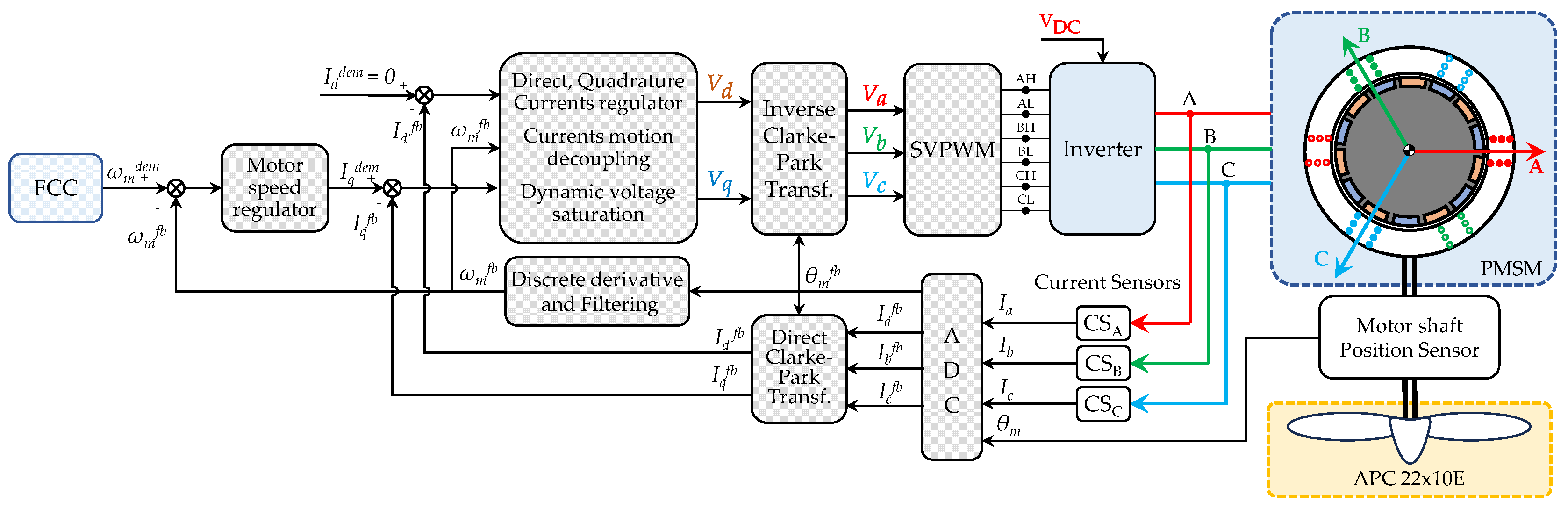
Figure 4.
MIL algorithm design and implementation workflow.
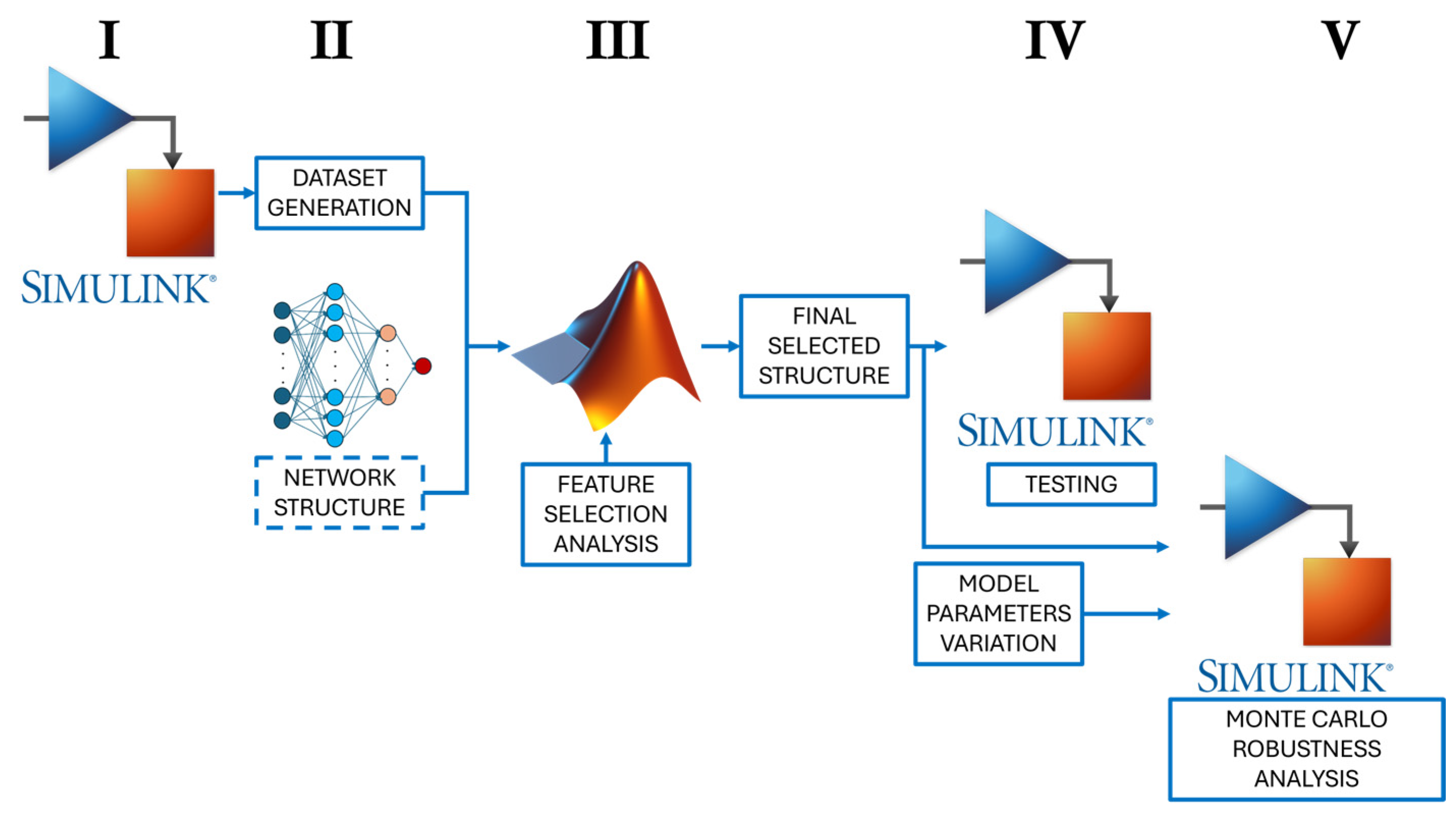
Figure 5.
Neural network architecture.
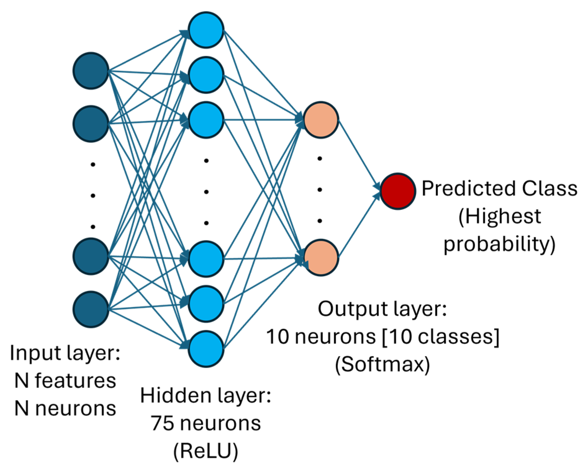
Figure 6.
Flowchart of the isolation algorithm.
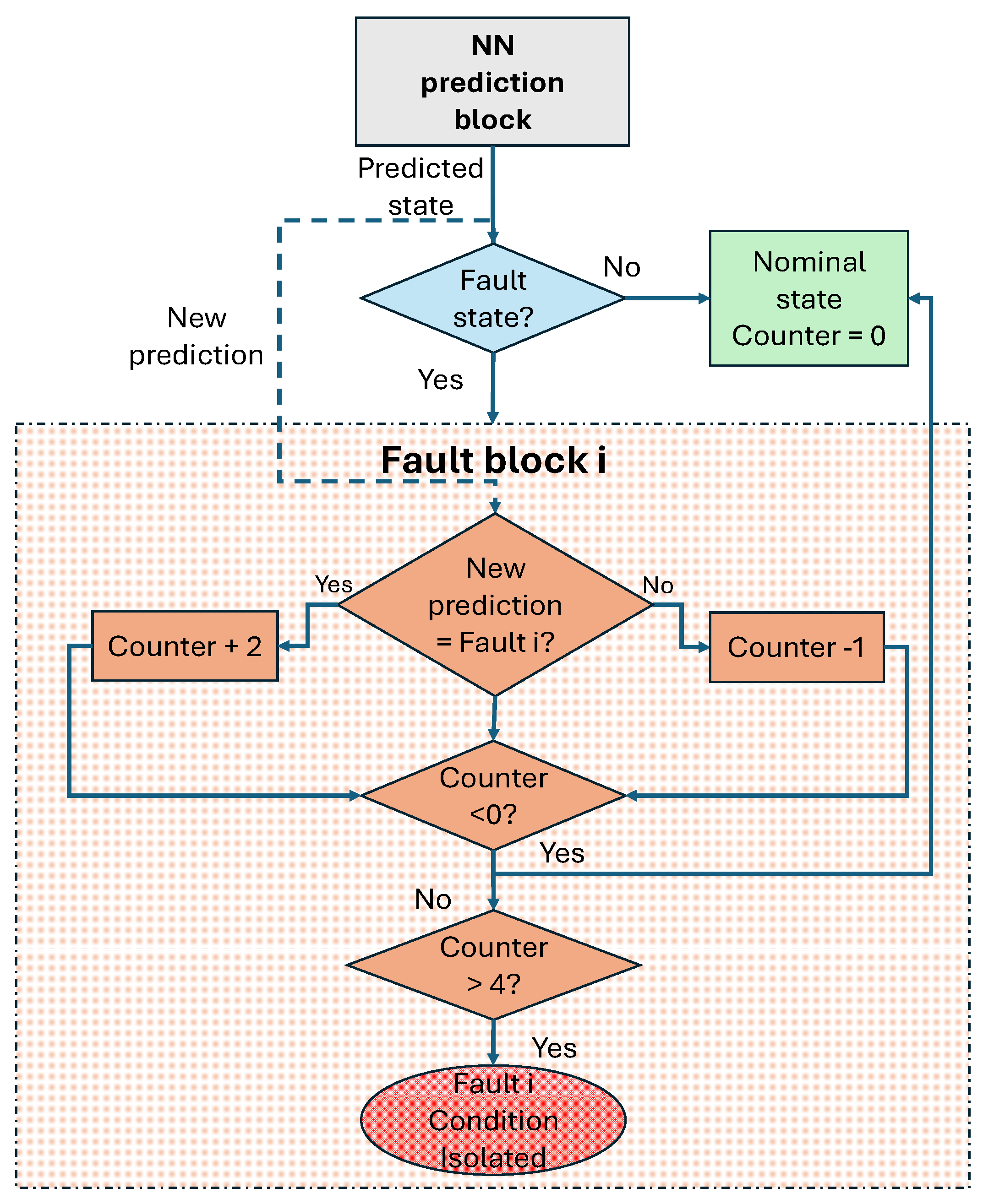
Figure 7.
Hidden layer size sensitivity analysis in terms of train, validation and test accuracy.
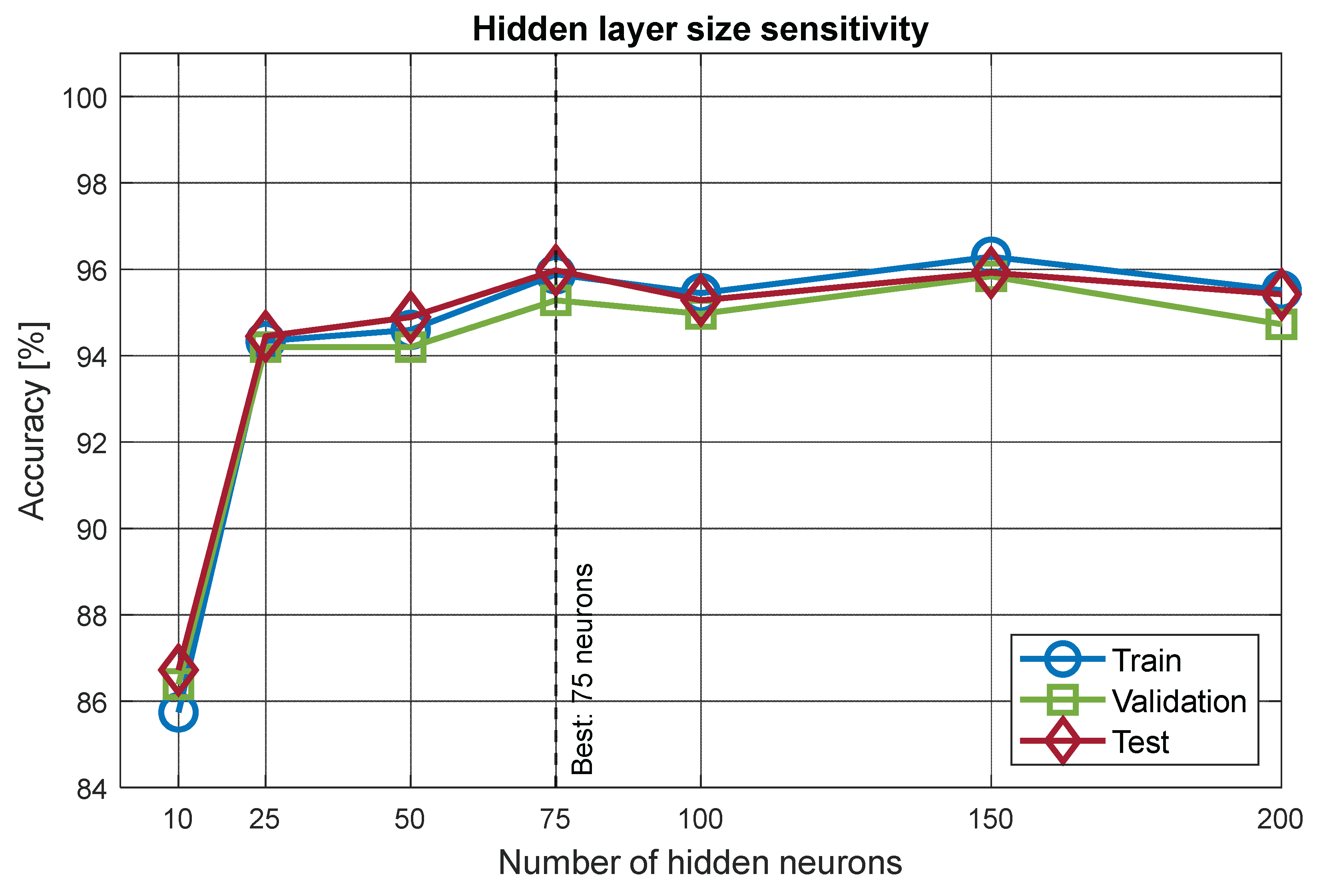
Figure 8.
Feature selection analyses. Validation accuracy percentage is reported. Green highlighted cells indicate features included in the considered subset.
Figure 8.
Feature selection analyses. Validation accuracy percentage is reported. Green highlighted cells indicate features included in the considered subset.
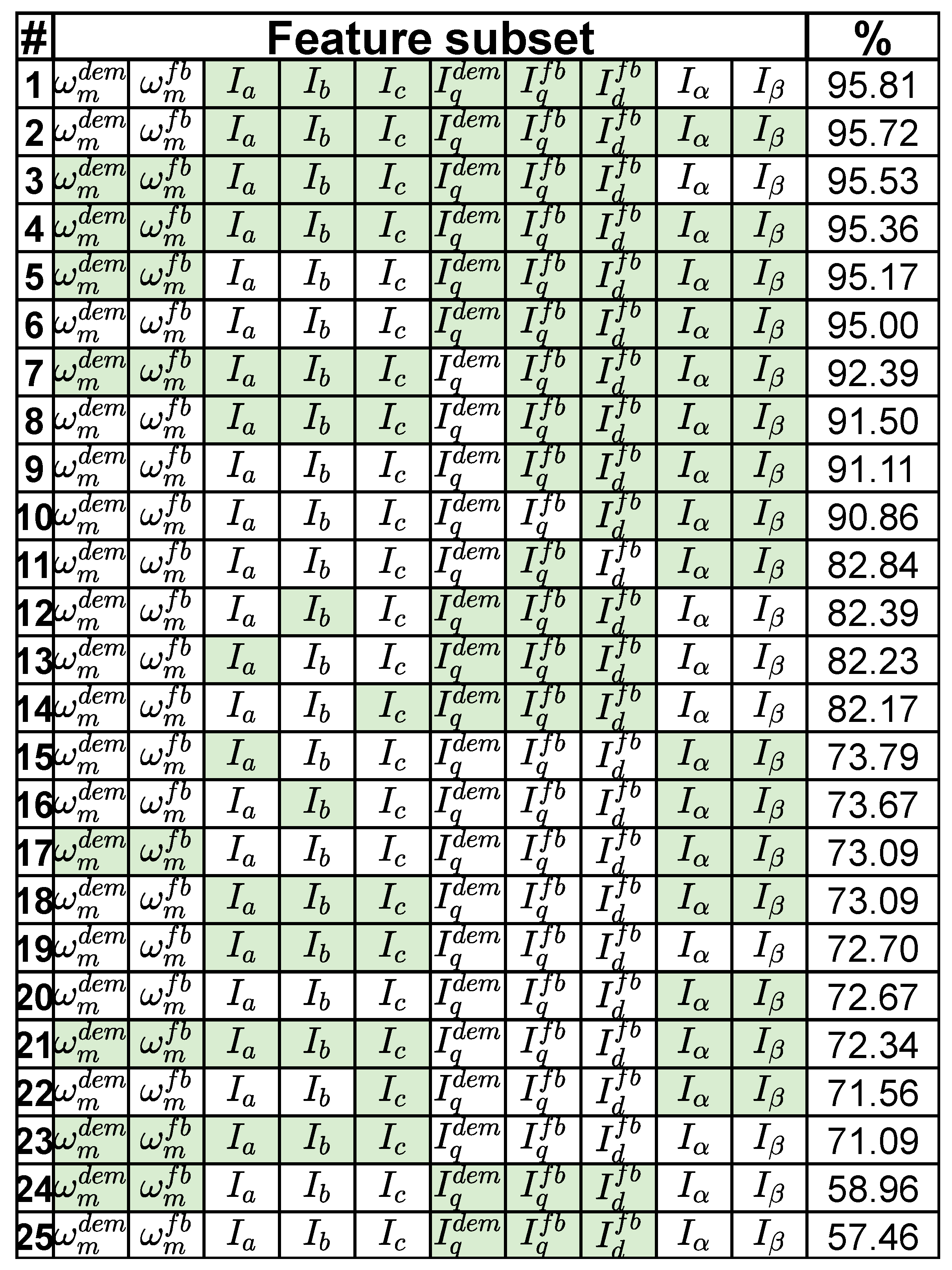
Figure 9.
Current (top); Actual injected state vs isolated (middle); Fault counter (bottom). Zoom, normalized current. High phase A MOSFET fault (left); low phase A MOSFET fault (center); Open phase A MOSFETs fault (right).
Figure 9.
Current (top); Actual injected state vs isolated (middle); Fault counter (bottom). Zoom, normalized current. High phase A MOSFET fault (left); low phase A MOSFET fault (center); Open phase A MOSFETs fault (right).
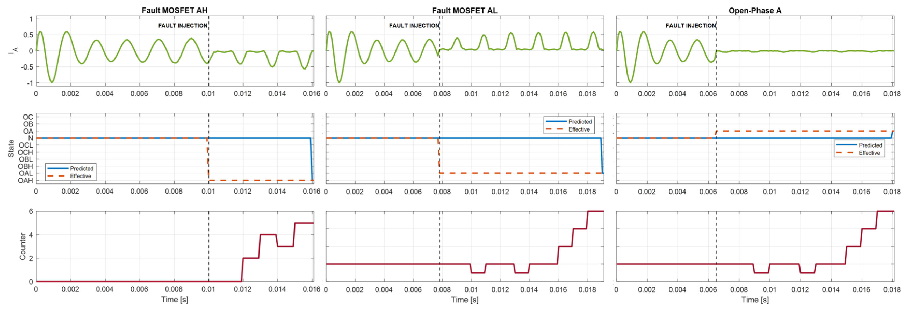
Figure 10.
Confusion matrix of the trained NN on the MIL simulation test for the ten operating conditions. Class-wise true positive rate (TPR) and false negative rate (FNR) are included. Instances expressed in percentage (left). Class-wise precision (P) and F1-score (F1) are included. Instances expressed in terms of absolute counts (right).
Figure 10.
Confusion matrix of the trained NN on the MIL simulation test for the ten operating conditions. Class-wise true positive rate (TPR) and false negative rate (FNR) are included. Instances expressed in percentage (left). Class-wise precision (P) and F1-score (F1) are included. Instances expressed in terms of absolute counts (right).
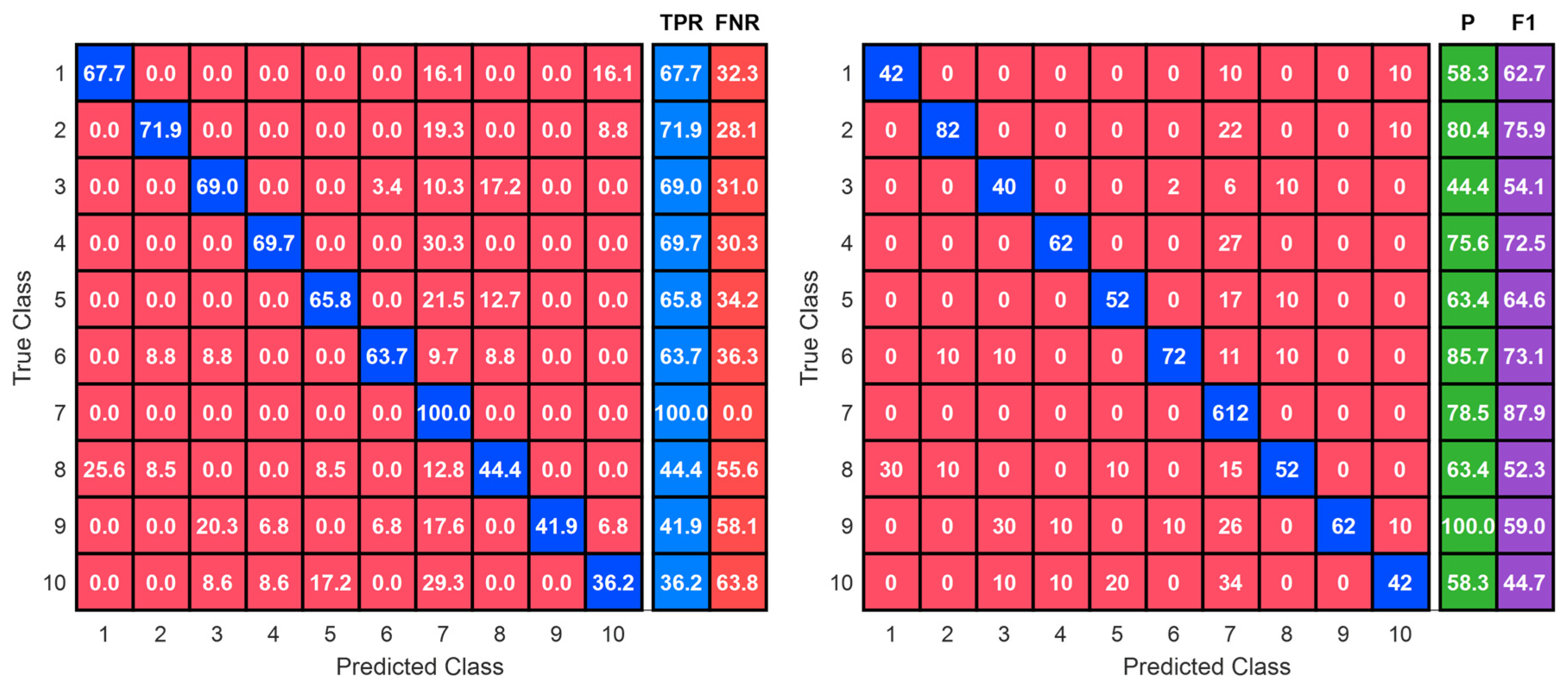
Figure 11.
Monte Carlo parameter distributions: phase resistance R (left) and phase inductance L (right).
Figure 11.
Monte Carlo parameter distributions: phase resistance R (left) and phase inductance L (right).
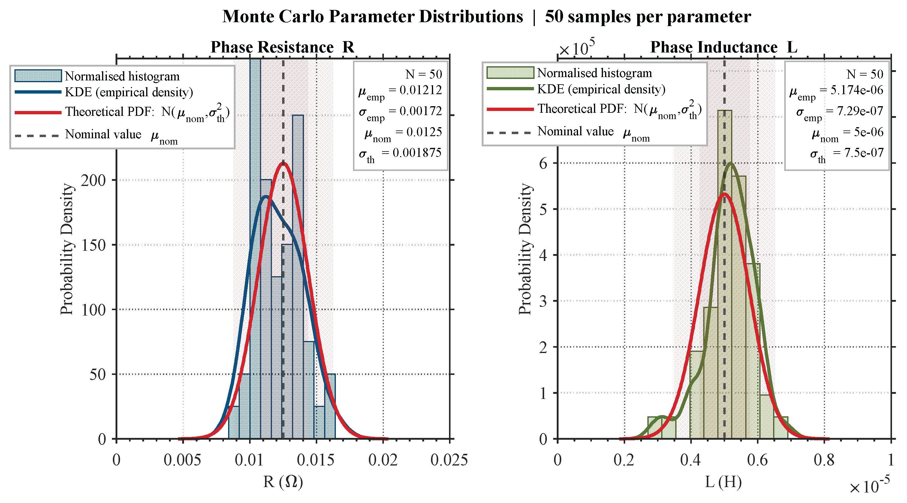
Figure 12.
Per-class metrics across all runs for each of the ten operating classes in Monte Carlo MIL simulation.
Figure 12.
Per-class metrics across all runs for each of the ten operating classes in Monte Carlo MIL simulation.
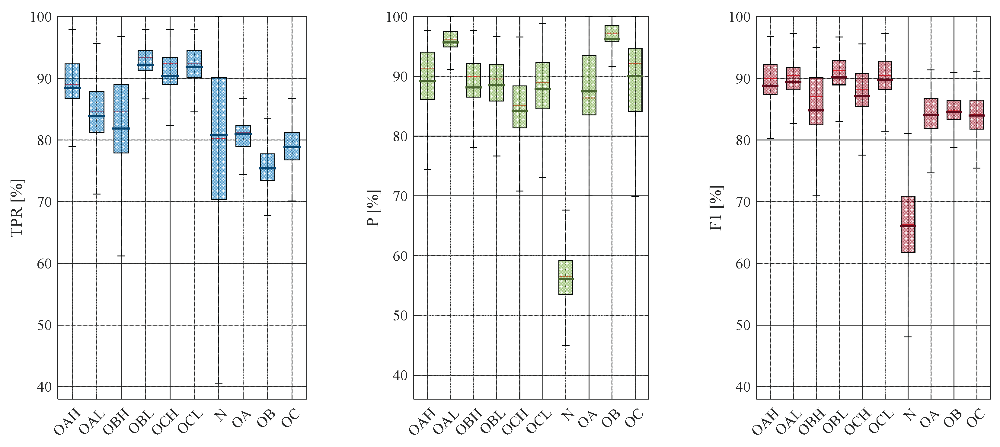
Figure 13.
Confusion matrix of the trained NN on the Monte Carlo MIL simulations for the ten operating conditions. Class-wise true positive rate (TPR) and false negative rate (FNR) are included. Instances expressed in percentage.
Figure 13.
Confusion matrix of the trained NN on the Monte Carlo MIL simulations for the ten operating conditions. Class-wise true positive rate (TPR) and false negative rate (FNR) are included. Instances expressed in percentage.
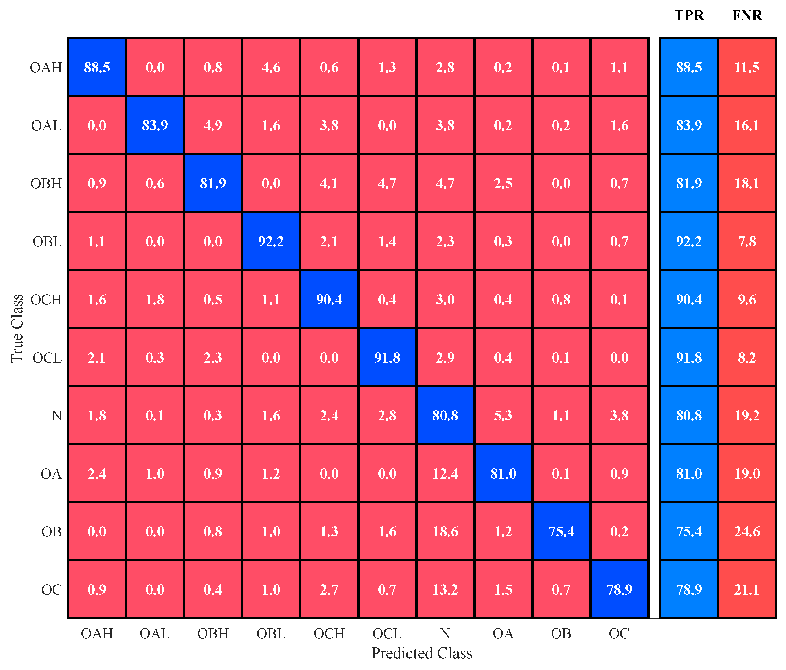
Figure 14.
Confusion matrix of the trained NN on the Monte Carlo MIL simulations for the ten operating conditions. Class-wise true positive rate (TPR) and false negative rate (FNR) are included. Instances expressed in terms of absolute counts.
Figure 14.
Confusion matrix of the trained NN on the Monte Carlo MIL simulations for the ten operating conditions. Class-wise true positive rate (TPR) and false negative rate (FNR) are included. Instances expressed in terms of absolute counts.
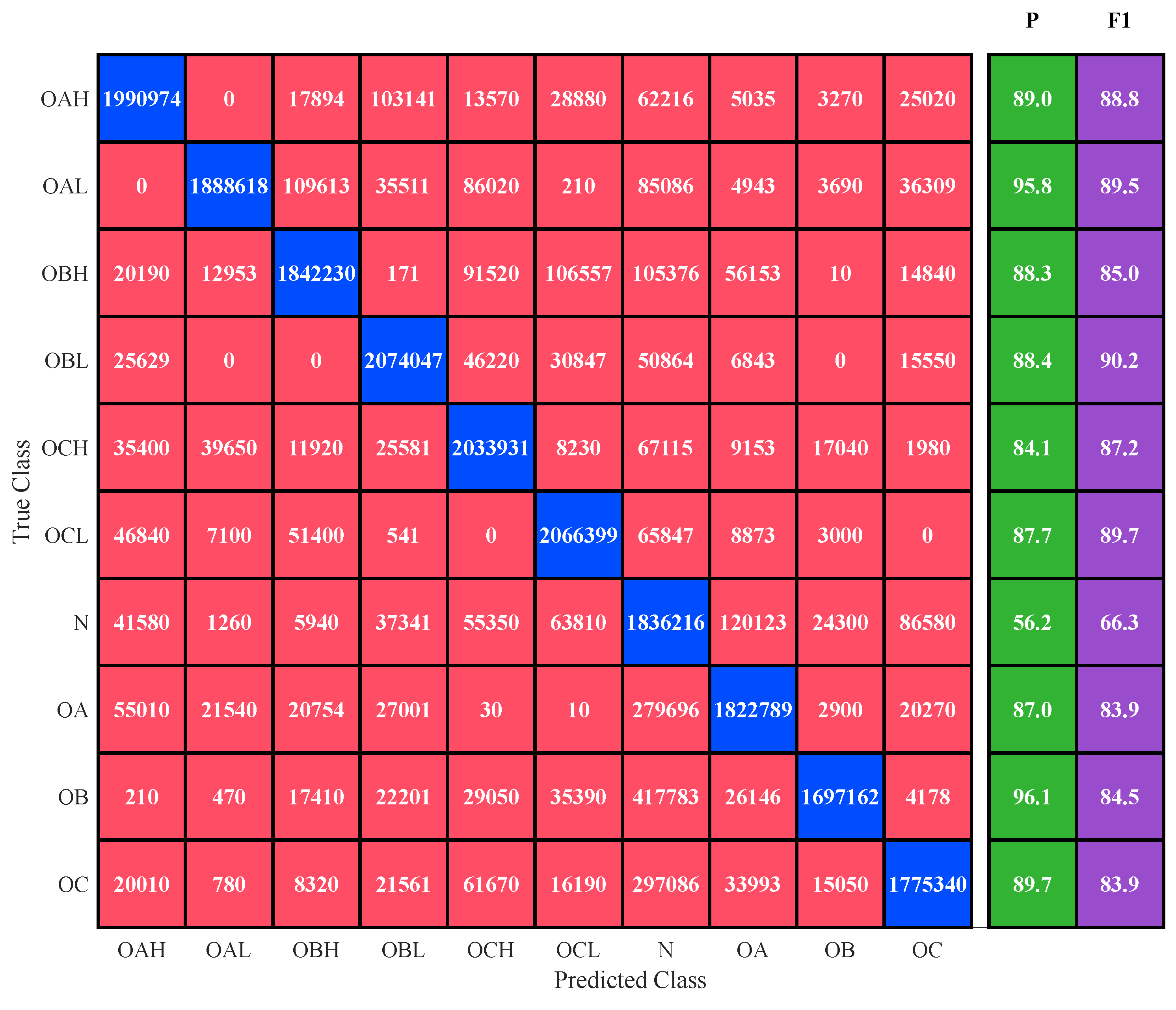
Figure 15.
Scatter plots with correlation of TPR, Precision and F1-score with respect to MC parameters: phase resistance (top); phase inductance (middle), torque constant (bottom).
Figure 15.
Scatter plots with correlation of TPR, Precision and F1-score with respect to MC parameters: phase resistance (top); phase inductance (middle), torque constant (bottom).
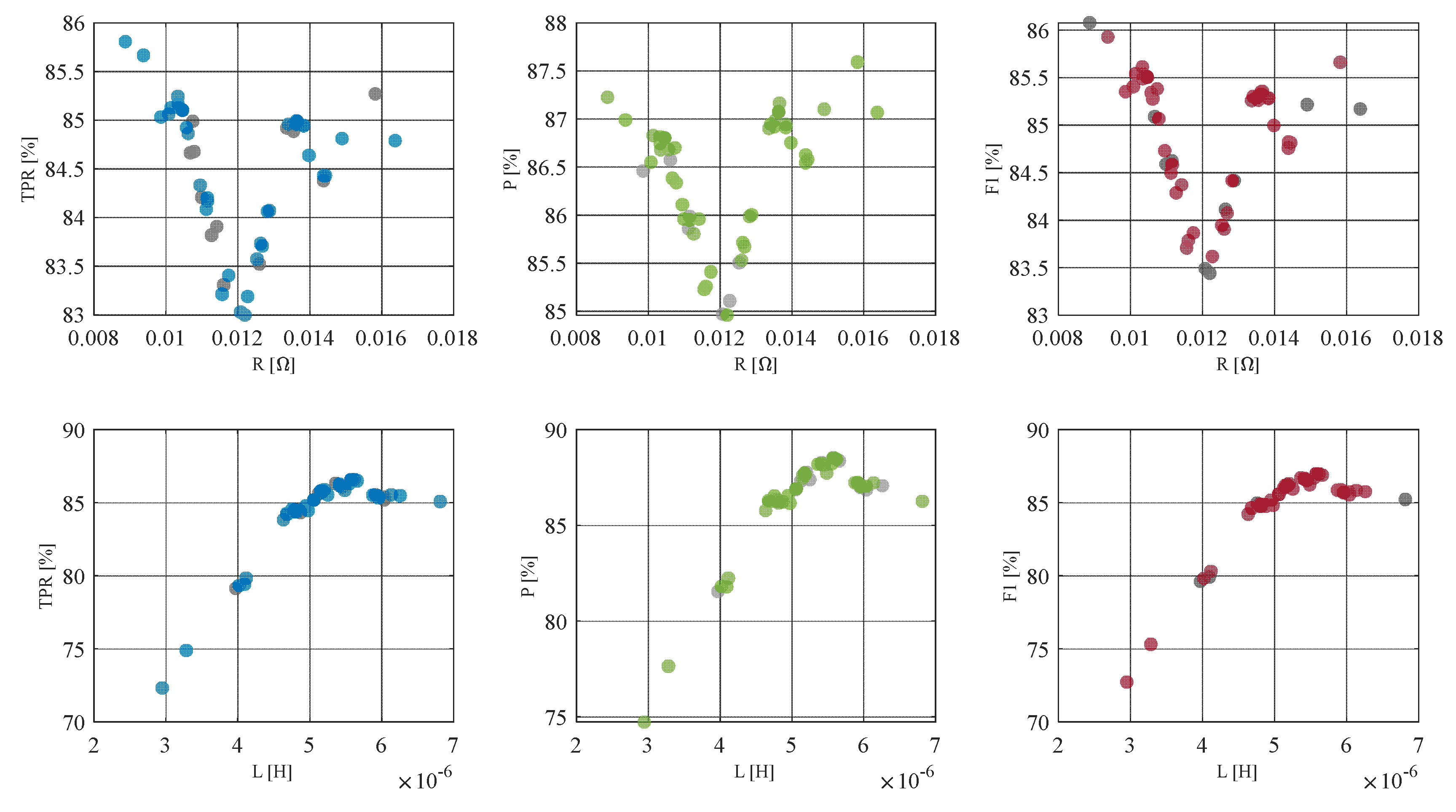
Figure 16.
Class-wise fault isolation time.
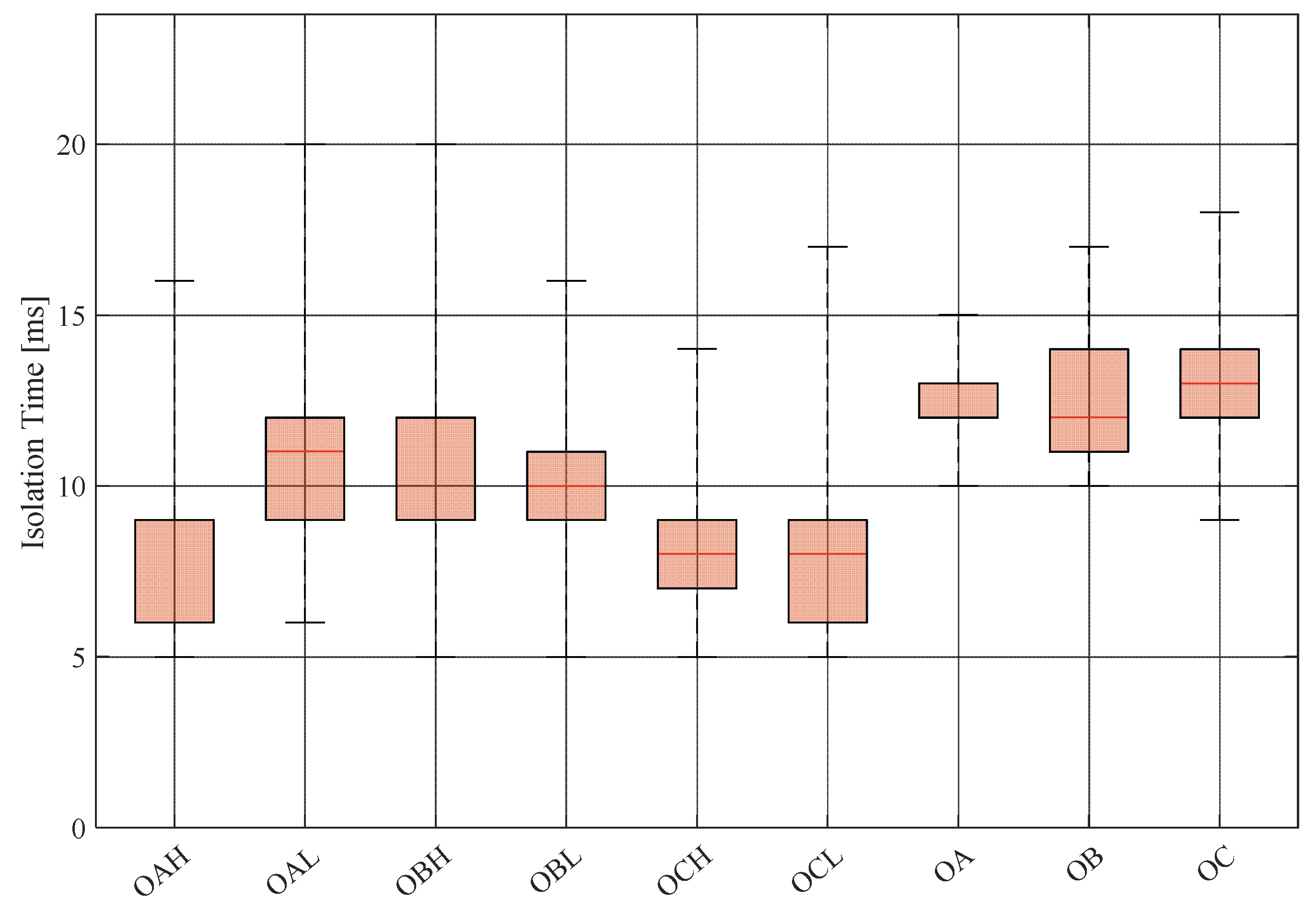
Figure 17.
Mean fault isolation time vs parameters variation.
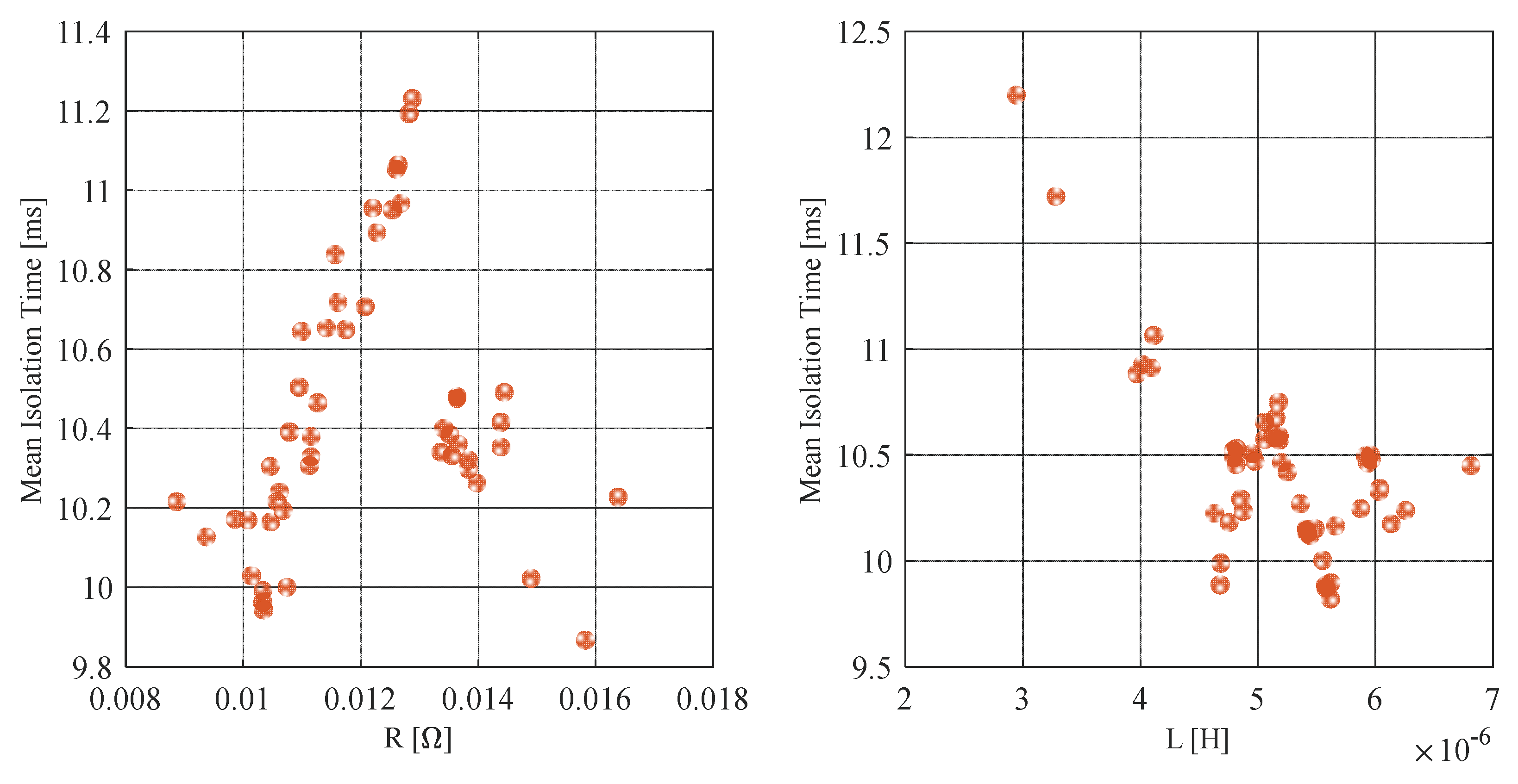
Figure 18.
Best and worst 5% Monte Carlo runs by F1-score, as function of phase resistance R and phase inductance L.
Figure 18.
Best and worst 5% Monte Carlo runs by F1-score, as function of phase resistance R and phase inductance L.
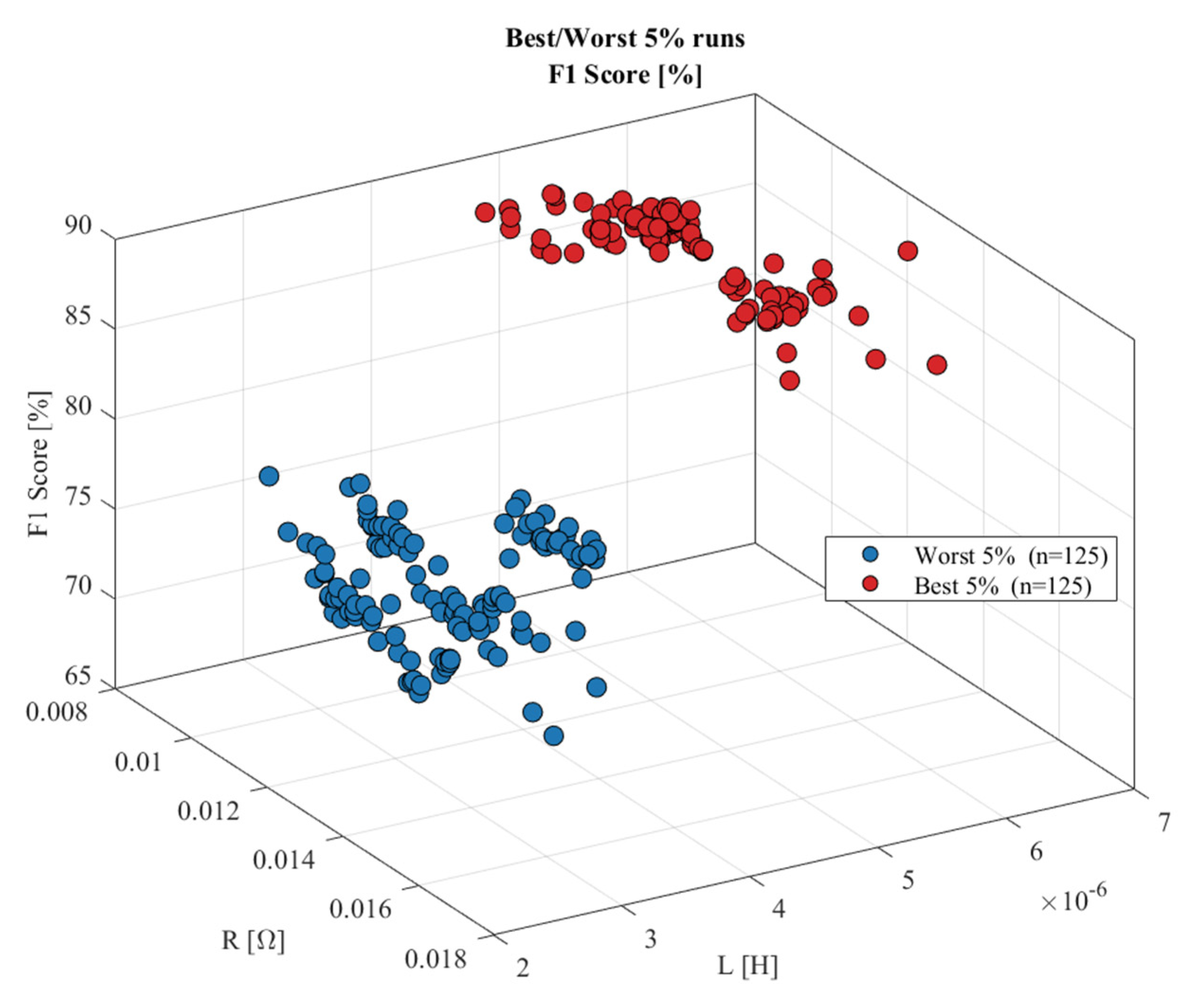

Table 1.
Fault class labeling.
| Operating condition [H: high side MOSFET High; L low side MOSFET; O: open; A, B, C: phase A, B, C; N: nominal] | Label |
| OAH | 1 |
| OAL | 2 |
| OBH | 3 |
| OBL | 4 |
| OCH | 5 |
| OCL | 6 |
| N | 7 |
| OA | 8 |
| OB | 9 |
| OC | 10 |
Table 2.
Simulator parameters setting for dataset generation.
| Parameter | Value | Unit |
| Numerical integration time step | 10-7 | s |
| PWM activation time step | 5 x 10⁻⁵ | s |
| Simulation duration | 0.2 | s |
| Fault injection time | 0.1 | s |
| Operational speed range | From 5800 to 7100 | rpm |
Table 3.
Neural network hyperparameters.
| Parameter | Value | Motivation |
| Network architecture | Feedforward fully connected | Simple architecture suitable for real-time embedded implementation |
| Input layer | Variable size | Adapted to selected feature subset under evaluation |
| Hidden layers | 1 | Reduces computational complexity while retaining sufficient learning capability |
| Hidden neurons | 75 | Empirically identified as best trade-off between classification accuracy and network size |
| Hidden activation | ReLU | Fast convergence and mitigation of vanishing gradient issues |
| Output layer activation |
Softmax | Computes class probabilities for multiclass task |
| Output layer | 10 | Number of available classes |
| Optimizer | Adam | Efficient gradient-based optimization with adaptive learning rate |
| Mini-batch size | 32 | Trade-off between convergence stability and computational efficiency |
| Maximum epochs | 800 | Upper limit for training iterations |
| Early stopping | Validation-based | Prevents overfitting when validation performance no longer improves |
Table 4.
Simulator parameters setting for MIL FDI algorithm testing.
| Parameter | Value | Unit |
| Numerical integration time step | 10-7 | s |
| PWM activation time step | 5 x 10⁻⁵ | s |
| Simulation duration | 0.05 | s |
| Random fault injection time range | From 0.005 to 0.01 | s |
| Operational speed | 6350 | rpm |
Table 5.
Simulator parameters setting for Monte Carlo MIL FDI algorithm testing.
| Parameter | Value | Unit |
| Numerical integration time step | 10-6 | s |
| PWM activation time step | 5 x 10⁻⁵ | s |
| Simulation duration | 0.1 | s |
| Fault injection time | 0.01 | s |
| Operational speed | 6350 | rpm |
| Speed step time | 0.04 | s |
| Commanded speed step | 6550 | rpm |
Table 6.
Hidden layer size analysis, open-phase class wise test accuracy.
| Hidden layer size | OA | OB | OC |
| 10 | 78.5% | 76.5% | 78.4% |
| 25 | 88.5% | 82% | 81.9% |
| 50 | 85.5% | 82.5% | 85.9% |
| 75 | 87.5% | 87% | 85.4% |
| 100 | 85.5% | 81.5% | 77.9% |
| 150 | 89.5% | 85.5% | 85.4% |
| 200 | 88.5% | 82% | 80.4% |
Disclaimer/Publisher’s Note: The statements, opinions and data contained in all publications are solely those of the individual author(s) and contributor(s) and not of MDPI and/or the editor(s). MDPI and/or the editor(s) disclaim responsibility for any injury to people or property resulting from any ideas, methods, instructions or products referred to in the content. |
© 2026 by the authors. Licensee MDPI, Basel, Switzerland. This article is an open access article distributed under the terms and conditions of the Creative Commons Attribution (CC BY) license (http://creativecommons.org/licenses/by/4.0/).
Copyright: This open access article is published under a Creative Commons CC BY 4.0 license, which permit the free download, distribution, and reuse, provided that the author and preprint are cited in any reuse.