
Submitted:
18 September 2026
Posted:
20 September 2026
You are already at the latest version
Abstract
Aiming at the problem of sea clutter suppression and dim target detection in sea clutter, a sea clutter identification method based on detection sliding window convolutional neural network ( DSW-CNN ) model is proposed. Firstly, the characteristics of sea clutter are analyzed to obtain the characteristics that can distinguish sea clutter and target. Then, the fully polarized radar signal is converted into graph data, and the sea clutter is initially suppressed by using the spatial and temporal characteristics of the graph data. Finally, the proposed DSW-CNN model is used to extract and classify the feature of the graph data nodes, so as to realize the target identification in the background of sea clutter. The proposed method is simulated and analyzed by using experimental data. Experiments show that the proposed method can achieve a detection probability of 98 % when the target signal-to-clutter ratio is less than 12 dB, and the parameter scale of the lightweight model is reduced to 10 % of the original model. The proposed model provides some support for sea clutter suppression theory and engineering implementation.
Keywords:
sea clutter
; target identification
; lightweight network
; convolutional neural network
; full polarization
; detection of sliding window
1. Introduction
The marine environment is different from the land environment. It is affected by weather, tide, earth rotation and other aspects. The randomness and complexity of the sea clutter generated by the sea clutter are much larger than those of the land clutter. The detection of sea targets is widely involved in military and civil fields. Anti-sea clutter interference is one of the main problems faced by sea surface target detection and recognition technology.
Therefore, how to effectively and reliably detect and identify sea targets in the background of sea clutter is a key technology that needs to be studied. Constant False Alarm Rate (CFAR) [1] is a common adaptive algorithm used in radar systems to detect target echoes in the background of noise, clutter and interference. However, the adaptability of low observable target detection in the background of sea clutter needs to be further improved.
In recent years, deep learning and artificial intelligence technologies have flourished. Convolutional Neural Network (CNN) [2], Deep Belief Network (DBN) [3], Recurrent Neural Network (RNN) [4], etc., are currently widely used to detect targets, providing a new idea for sea clutter suppression.
It is an effective solution to suppress sea clutter by identifying targets and interference. Aiming at the problem of sea clutter and target identification, this paper proposes a sea clutter identification technology based on detection sliding window convolutional neural network (DSW-CNN) model. Firstly, the characteristics of sea clutter are analyzed to obtain the characteristics that can distinguish sea clutter and target. Then, the fully polarized radar signal is converted into graph data, and the sea clutter is initially suppressed by using the spatial and temporal characteristics of the graph data. Finally, through the method of knowledge distillation, an efficient and small-scale network model, namely the lightweight convolutional neural network based on detection sliding window (LDSW-CNN) model, is obtained, and the model is used to extract and classify the feature of the graph data nodes, so as to realize the target identification in the background of sea clutter, which can provide theoretical reference and technical support for subsequent deployment to edge equipment.
In the field of maritime target detection, the current mainstream engineering application method is based on the CFAR algorithm. The principle of this method is simple and easy to implement. For different clutter backgrounds, many scholars have proposed many CFAR variants, such as CA-CFAR, SO-CFAR, GO-CFAR. However, the applicability of the CFAR-based method in the case of low signal-to-clutter ratio needs to be further improved. With the continuous development of artificial intelligence technology, many scholars have begun to use deep learning methods to design marine target detectors to improve the accuracy of target detection. Since AI godfather Hinton proposed knowledge distillation technology, knowledge distillation has received extensive attention from researchers and has shown great research value in network compression.
In 2014, Hinton et al.first proposed the concept of knowledge distillation [15], and verified its effectiveness and feasibility in convolutional neural network compression through experiments. Knowledge distillation strategy has played a role in many computer vision applications such as object detection, semantic segmentation, object recognition, video classification, and image dehazing. The essence of knowledge distillation [16] is reflected in the fact that teachers will impart their own thinking process and summary as a kind of knowledge essence to students. Through understanding and learning, students can obtain abstract and refined knowledge to achieve the level close to teachers.
The basic idea of knowledge distillation is to let the convolutional neural network imitate human learning behavior, transfer the knowledge learned by the large network (teacher network) to the small network (student network), and guide the training of the small network, so as to realize the purpose of compressing the large network into the small network. It has become a trend to apply knowledge distillation to lightweight processing of deep learning models. If the complex deep learning neural network model can be successfully compressed into a small neural network through this method, the possibility of deploying the model to edge devices will be greatly improved.
Based on the constant false alarm rate detection algorithm, this paper uses convolutional neural network to identify sea targets and sea clutter, and constructs a new lightweight network model by network pruning. A convolutional neural network based on detection sliding window (DSW-CNN) and the identification technology of sea target and sea clutter are proposed. Compared with the constant false alarm rate detection, this method can adapt to more complex situations to improve the detection accuracy, and has intelligence. Compared with the traditional convolutional neural network model, it has lower hardware capacity requirements and smaller parameter model.
2. Polarimetric Radar Data Preprocessing
Under natural conditions, radar detects sea targets incorrectly. The main reason is that the amplitude generated by sea clutter, especially sea spikes, may be higher than the target echo signal. However, the characteristics of sea clutter signal and target signal in time and space are significantly different. Therefore, in this chapter, by preprocessing the sea detection polarization radar data and converting the polarization radar signal data into graphic data, the spatial amplitude morphological characteristics and time position change characteristics of the detection target can be effectively extracted.
2.1. The General Idea of Polarization Radar Signal Preprocessing
The polarization radar works in the staring mode, continuously transmitting and receiving signals in a fixed direction, thereby generating continuous echo signals of different distance units in the same direction. Each data unit in the polarization radar signal data can reflect the position information of the point and the echo information at a certain time.
Usually, the sea detection polarization radar is located at low altitude, away from the area where the target may exist. It is assumed that the target exists in the radar staring direction, within the radar detection range, and the target and the sea clutter scattering point are located in the same horizontal plane. In the radar sea detection mission, the signal detected by the radar is a one-dimensional signal, and the echo signal is continuously collected through long-term operation. The sea detection radar signal is described as multi-frame data , involving two dimensions, which R is the distance unit, K is the number of frames, and R is the real set symbol.
2.2. Graph Data Transform
The polarization radar works in the staring mode, continuously transmitting and receiving signals in a fixed direction, thereby generating continuous echo signals of different distance units in the same direction. Each data unit in the polarization radar signal data can reflect the position information of the point and the echo information at a certain time. In the sea detection radar signal, most of the data units contain sea clutter echo signals. However, because the effective reflection area (RCS) of the target is larger than that of the sea wave, the characteristics of the target echo signal will cover most of the characteristics of the sea clutter signal. Therefore, on the distance unit where the target is located, it can be regarded as no sea clutter signal exists. Su et al.proposed a method for extracting targets from scanning radar data [23]. This paper refers to this method to perform graphic data conversion processing on staring radar data. Since the target and strong clutter echo signals (such as sea spikes) occupy multiple adjacent small areas, each frame of the radar signal is subjected to a threshold-based detection process. In a frame, the target echo signal has a certain width and occupies several continuous range units. If the continuous echo signal with an amplitude exceeding the threshold is considered as a sample, a node in the graphic data of the frame is obtained. The characteristics of each node include the center distance unit of the correlation unit and the signal characteristics. In continuous frames, the target echo signal is continuous, and the strong clutter signal is random. Node correlation between frames can effectively reduce the interference of strong clutter signals. The overall process of data preprocessing is shown in Figure 1.
2.2.1. Low Threshold Detection Processing
Threshold detection is performed on each frame of the radar signal , and the detection threshold of the frame is determined by the specific data of each frame.
Among them, is the constant false alarm rate, the value is set to 10-2. The function sort() is to sort each frame of echo in descending order. A new set of data is obtained after descending order. The Tk value is the 0.01 * R term of .
After each frame is processed, an array can be obtained.
Here, r and k are the indexes of the data unit, which means that the data is the data of the rth distance unit in the kth frame.
2.2.2. Connectivity Detection Processing
Threshold detection is performed on each frame of the radar signal . The specific data of each frame determines that the detection threshold of the frame is 0 and 1 matrix after low threshold detection. It can be considered that the data with a value of 1 is the data of interest, and its confidence for the target is higher. Because the target echo signal is continuous, it is considered that multiple continuous data with a value of 1 in a frame come from the echo information of a target. Through connectivity detection, it can avoid judging continuous data with a value of 1 as different targets, improve its detection accuracy, and reduce unimportant information input.
By detecting the connectivity of each frame , n connected components can be obtained, and n nodes in the corresponding frame can be detected.
Here, ni is the number of nodes in frame i, and n is the total number of nodes in this group of data. Two eigenvalues of space-time auxiliary features and signal features can be obtained from each node.
2.2.3. Spatio-Temporal Auxiliary Feature Extraction Processing
The spatio-temporal auxiliary feature is composed of the center distance ri unit of the node, the number of frames ki and the size of each node ci.
Because the sea detection radar does not need to consider the influence of azimuth angle in the staring mode, but due to the influence of sea clutter, the target and false alarm samples span multiple continuous units in the distance dimension, or the nodes representing the same target between frames are different in size. Therefore, the signal characteristics of the nodes are one-dimensional.
2.2.4. Correlation Detection Processing
In multi-frame data, the target echo signal and sea clutter signal can be better identified by the correlation of nodes between frames. The node representing the target echo signal exists near the same position of the adjacent frames. It can be considered that when the target velocity represented by the echo signal is less than or equal to 10m / s, the echo signal is the target signal, and the adjacent two frames are associated.
Among them, the upper limit of Vij is 5, which is the value of 10m/s after converting from the real distance to the distance unit, indicating that the absolute value of the difference between the node center distance unit of two adjacent frames is less than or equal to 5.
3. Design of Intelligent Identification Model Based on Lightweight Network
The convolutional neural network (CNN) in deep learning has a wide range of applications. Its principle is mainly to extract features through the convolutional layer, the pooling layer reduces the data size, the activation layer performs data filtering, and the full-link layer transforms multi-dimensional feature data into one-dimensional feature data to construct an objective function. By reducing the residual error, it is trained as a network model that can realize the identification of the target and the sea clutter. However, the traditional convolutional neural network model, which is large in scale, has multiple convolutional layers, pooling layers, and activation layers. It has a large amount of computation and extremely high requirements for computing power. According to the different tasks, different network structures are adopted, and the U-Net network structure performs well for image segmentation tasks. In this paper, a convolutional neural network based on detecting sliding windows (DSW-CNN) is proposed based on the U-Net network structure. Through the detection method similar to the constant false alarm rate, the convolution kernel is designed according to the working principle of the detection sliding window in CFAR, which makes the network model more interpretable, integrates more data features, and has smaller parameter scale and faster running speed.
3.1. The Overall Structure of DSW-CNN Target Identification Model
The convolutional neural network model refers to a network model mainly composed of convolutional layers. When processing graphic data, the input graphic data has three attributes, indicating the need for a dedicated model architecture. First, the data is high-dimensional. The typical image of the classification task contains 224 × 224 RGB values (i.e., 150,528 input dimensions). If the CFAR algorithm is implemented using a fully-linked network, the hidden layer is usually larger than the input size, so even for shallow networks, the weight number will exceed 15,5282 or 22 billion. This brings obvious practical problems in the required training data, memory and computation. Secondly, in the real situation, the location and environment of the target will not affect the characteristics of the target too much. For example, if a target is placed in any position within the radar detection range, it will not affect the conclusion that ' this is the target '. However, its different positions in the echo signal are completely different data inputs for the computer. If you want to make the constant false alarm rate detection algorithm applicable to targets in various positions, you need to set multiple threshold factors corresponding to different situations, which is obviously inefficient and difficult to achieve in reality.
The convolutional layer of the convolutional neural network uses parameters shared throughout the image to process each local image region independently. Compared with fully linked layers, they use fewer parameters, exploit the spatial relationship between nearby pixels, and do not have to relearn the pixel interpretation at each location. Figure 2 shows the structure of the DSW-CNN model. Since the activation layer does not change the size of the data, the activation layer and the convolution layer are combined into one layer.
Through knowledge distillation, the knowledge of the trained complex teacher network is transferred to a simpler student network [25]. Figure 3 shows the student network LDSW-CNN designed by pruning [26]. Teachers ' network and students ' network are composed of coding layer, decoding layer, post-processing layer and output layer. The coding layer can extract the features of the input data, so it can be called the signal feature extraction network. The decoding layer can analytically output the eigenvalues obtained by the coding layer, so it can be called the signal feature analysis network. The post-processing layer and the output layer are the final output of the results obtained by the decoding layer to obtain visual detection result information, so it can be called the detection result output network. The following will discuss these three parts and the lightweight process.
3.2. Signal Feature Extraction Network Design
The signal feature extraction network of DSW-CNN network model is composed of convolution layer, activation function and maximum pooling layer. The convolution layer design, the maximum pooling layer design and the activation function design are discussed respectively.
3.2.1. Convolution Layer Design
The convolution layer is a network layer based on convolution operation. This paper first studies the convolutional neural network model applied to single-frame radar echo signals, namely one-dimensional data convolutional neural network (1D-CNN) [27]. In one dimension, convolution converts the input vector x into the output vector z, so each output is a weighted sum of nearby inputs. Each position uses the same weight, collectively referred to as a convolution kernel or filter. The area where the input is weighted and summed is called the kernel size. For a kernel of size 3, the output value can be obtained.
Among them, ω = ω1, ω2, ω3 are convolution kernels. The convolution operation is equivalent to the translation. If the input x is translated, the corresponding output z is translated in the same way. In the convolution process, the size, translation step and expansion method need to be set for the convolution kernel.
The size of the convolution kernel determines the number of input x in a convolution, the translation step size determines the size of the output z, and the expansion rate can artificially design the convolution kernel to a certain extent. In order to compare the CFAR algorithm of one-dimensional data. The DSW-CNN model is designed to have a convolution kernel size of 5, a step size of 1, and an expansion rate of 1. The convolution layer composed of the convolution kernel, as shown in Figure 4.
Among them,X is the input layer, Z is the output layer, W2 is the detection unit, the term of 0 is the protection unit, W1 and W3 are the reference units, and their values correspond to the threshold factors in the CFAR algorithm. Since the convolution kernel operation is started by the center of the convolution kernel to align the first item, the problem of out-of-edge detection will occur. The filling scheme of the convolution layer of the DSW-CNN model adopts zero filling to ensure that the output data size is consistent with the input data size. Through multi-layer design and multiple iterative training, the network model will have multiple W1 and W3 to adapt to different sea conditions.
The convolution layer calculates its output by convolution input, adding bias β and passing each result through the activation function . When the kernel size is 5, the stride is 1, and the expansion rate is 1, the ith hidden unit is
Here, the bias β and the kernel weights ω1, ω5 are trainable parameters, ω2, ω4 are 0, ω3 is -1, and (filled to zero) when the input x exceeds the effective range, we regard it as zero.
If only one convolution is used, the information will inevitably be lost. In this paper, the nearby inputs are averaged, and the results less than zero are cut by the Leaky ReLU activation function. Therefore, multiple convolution kernels are set in one convolution layer for parallel computing. Each convolution produces a new set of hidden variables, namely feature maps. Each row of the feature map corresponds to an area in the previous layer, and the area size is the receptive field. In a given convolutional layer, the receptive field size is :
Here, K is the size of the convolution kernel (for example, K = 3 corresponds to the convolution kernel of 3x3). S is the step size, which represents the interval of the convolution kernel sliding on the input feature map (for example, S = 1 represents one unit of sliding each time, and S = 2 represents two units of sliding each time).
In the convolutional neural network (CNN), the eigenvalues of each layer are only connected to a local area of the previous layer, which gradually expands as the network level deepens, as shown in Figure 5.
In the one-dimensional sequence with input data of 9 × 1, the first hidden layer of 9 × 3 can be obtained by using three convolution kernels of 5 × 1 in the first layer, and the second hidden layer can be obtained by using three convolution kernels of 5 × 3 in the first hidden layer. Each row eigenvalue of the second hidden layer can correspond to the value of the input data weighted by different weights, and the receptive field of each row is 9.
In the two-dimensional graphics data, the convolution layer principle is similar to the convolution principle of the above one-dimensional data. Now, a two-dimensional data composed of Xij is used as input data, and 8 convolution kernels of 5 × 5 size are used for convolution operation to obtain its hidden layer.
Wmn is a set of convolution kernels. This is just the weighted sum of a 5×5 rectangular input region. The convolution kernel is translated horizontally and vertically in the two-dimensional input data, and an output value is generated at each position. Its receptive field is the same as the convolutional neural network principle of one-dimensional data.
Whether the input data is one-dimensional data or two-dimensional data, in order to enable an eigenvalue to ' see ' more input layer information, multi-layer convolution is needed. The proposed network model sets the input data as a one-dimensional sequence of 80 × 1, which is represented as a fragment of 80 consecutive distance units in a frame. Because after the above graph data conversion, the block of interest is extracted, and the size of each block is not more than 80×80, it can be considered that in the 80×80 data, it can contain a block of interest. Subsequently, through model training, it is sufficient to identify target echo and sea clutter for 80×80 data.
In the signal feature extraction layer of the DSW-CNN network, a 5×5 convolution kernel is used, and its expansion rate is 1, which enables the network model to obtain a larger range of data features at one time. In the LDSW-CNN network, due to the pruning method, in order to reduce the parameter scale, only one convolutional layer is used, sacrificing the depth of the network. Therefore, its convolution kernel size is set to 3×3, and the expansion rate is 1 to obtain more accurate data features.
3.2.2. Pooling Layer Design
If data feature extraction is only performed through the stacking of convolutional layers, although the information loss of the input data is small, it will cause a sudden increase in calculation parameters and the calculation complexity is too large to meet the requirements of lightweight. Using the down-sampling strategy can effectively solve this problem. There are three common ways of down-sampling : sub-sampling, maximum pooling, and mean pooling. The pooling units of the DSW-CNN model and the LDSW-CNN model are both 2×2, and the step size is 2.
According to the design of convolution kernel and the principle of CFAR algorithm, the value obtained by each convolution is equivalent to the value after one detection. The maximum value selected in the pooling unit is to extract the value of the region that may be the target. After the convolution, it is the process of screening in all possible targets. Therefore, the DSW-CNN model selects the maximum pooling as the down-sampling method. The model adopts a structure similar to the U-Net network model in the coding layer, and inserts the maximum pooling layer between the convolutional layers.
The maximum pooling layer, also known as the maximum pooling operation, can extract the most important features from the feature map of the input layer, reduce the spatial dimension of the feature map, and reduce the amount of subsequent calculation. At the same time, it is beneficial to increase the receptive field so that each layer in the network can capture a wider range of context information. The use of the maximum pooling layer can also prevent overfitting. The maximum pooling layer reduces the spatial resolution of the feature map. Although some feature information is lost, the risk of overfitting of the network is reduced to a certain extent. It can also improve the gradient flow. When training the convolutional neural network model, the gradient may disappear or explode in the back propagation process. The maximum pooling layer helps to improve the gradient flow, so that the expected objective function can be obtained with fewer training times.
In the DSW-CNN model, the maximum pooling layer is placed after each convolution layer and activation function. In the LDSW-CNN model, only one maximum pooling layer is used. One is to extract more interesting features from the previous convolution, and form these eigenvalues into a new smaller-scale data. The other is to provide input data for the next convolution to reduce the subsequent computation.
3.2.3. Activation Function Selection
Between the convolutional layer and the maximum pooling layer, an activation function needs to be added. The activation function α(x) can play the role of threshold. The eigenvalues after convolution are judged by the activation function, which is similar to the threshold threshold T in the CFAR algorithm. The output is 1 when the output is greater than T, and 0 when the output is less than or equal to T. However, the use of activation function makes its output more diverse. The commonly used activation functions are as follows :
(1) Sigmoid function
The function is defined as :
If only through the function curve (Figure 6), its output value can be seen, and it has the characteristics of nonlinearity, monotonicity, continuity, smoothness and boundedness. Its output value can be used as a confidence level, but due to the exponential operation involved in the function, the computational resources required are large. Multiple uses of in the convolutional layer will lead to the problem of explosive growth of computation.At present, this function is rarely used in the hidden layer, and is often used in the final output layer when solving the binary classification problem.
(2) Tanh function
The function is defined as :
The function curve (Figure 7) is similar to the Sigmoid function curve. The value range of the function is (-1,1), and the output mean is 0, which can achieve similar functions as the Sigmoid function, but it is more fault-tolerant. There is still the calculation of the natural logarithm e in the function, and the large amount of calculation still exists.
(3) ReLU function
The function is defined as :
This function is a commonly used activation function, which is judged by comparing the input value with 0. It can make the value less than 0 unable to participate in the operation of the next layer, which can effectively reduce the subsequent calculation. This function is similar to the threshold threshold effect of CFAR algorithm, and can effectively realize the threshold threshold function of CFAR algorithm.
Figure 8.
Curve graph of ReLU function.
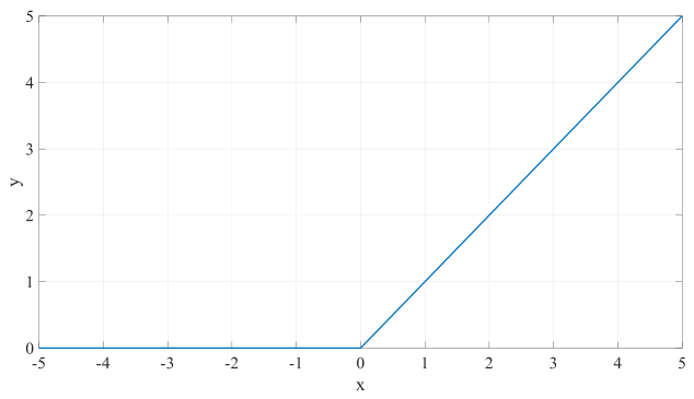
However, the DSW-CNN network needs to be applicable when the signal-to-clutter ratio is low. When the signal-to-clutter ratio of the target echo signal is low, the missed detection probability of the CFAR algorithm increases. Similarly, if the ReLU function is used as the activation function of the hidden layer, it is also difficult to improve the detection accuracy [28]. As a variant of the ReLU function, the Leaky ReLU function is expressed as :
Where α is a small positive slope (usually less than 1, e.g. 0.01), the output value is αx when x is less than 0, and x when x is greater than 0. This means that even if the input is negative, the Leaky ReLU function will output a small value (α times the input value), thus avoiding the problem that the target echo signal can not be output by sea clutter interference, resulting in missed detection. This function is the activation function of the hidden layer in DSW-CNN and LDSW-CNN.
The coding layer is subjected to multiple convolution-activation-maximal pooling, and finally the signal feature H1i ∈ R 10 × 10 × 32 is obtained.
3.3. Signal feature Analysis Network Design
The signal feature analysis network plays a role in mapping data from low dimensions to high dimensions in convolutional neural networks. This process is usually called upsampling or transposed convolution. The signal feature analysis network is mainly used for the following purposes :
1.Recovering spatial resolution
In the encoding stage of the convolutional neural network, the spatial size of the feature map is continuously reduced by pooling layer and convolution layer. The decoding layer gradually recovers this spatial resolution, allowing the network to reconstruct or upsample the feature map.
2. Reconstruction details
In the autoencoder, the decoding layer is used to reconstruct the details of the input data from the latent space or encoding, which can restore a part of the target signal that has not been extracted.
3.Segmentation and location
In image segmentation and target detection tasks, the decoding layer helps the network recover the structural information of the image from the feature representation to achieve accurate pixel-level positioning.
4. Feature fusion
In some network architectures, the feature maps of the decoding layer and the coding layer are fused to enhance the model 's utilization of the correlation between frames.
The signal feature analysis network of DSW-CNN consists of a transposed convolution layer and an activation function. The activation function in this network adopts the Leaky ReLU function which is consistent with the signal feature extraction network, and is no longer discussed separately. The following discussion is about the selection of upsampling strategy and the design of transposed convolutional layer.
3.3.1. Upsampling Strategy Selection
The maximum pooling layer in the feature extraction network is the down-sampling strategy. Up-sampling generally has four methods : equivalent expansion, maximum depooling, bilinear interpolation and transposed convolution. The first three methods can be regarded as the inverse process of pooling, and transposed convolution is similar to the use of reduced sampling with a step size of 2.
Equivalent expansion : This is the simplest upsampling method that doubles the size by copying each input cell or pixel four times. This method is fast but rough, because it does not introduce any new information, but simply enlarges the original data. If this is applied to the DSW-CNN network, the accuracy of the final output result will be reduced and the output target image will be blurred.
Maximum de-pooling : In the network where the coding layer uses the maximum pooling operation, the maximum pooled values are re-allocated to the same position where they originally come from (i.e., the position where the maximum value is located). Using this method, the target features will be scattered on the detection results, and the output targets are discontinuous.
Bilinear interpolation : This is a smoother upsampling method, which generates new pixel values by bilinear interpolation between input values. Bilinear interpolation takes into account the influence of surrounding pixels and generates a smoother and continuous image. However, this method will bring a large amount of calculation, and will make the output target larger than the real target range, and there is a big gap with the real target signal.
3.3.2. Transposed Convolution Layer Design
In the convolutional layer, if the convolution step size is 2, the output data size is half of the input data size. For the kernel size of 3, each output is the weighted sum of the three closest inputs. In transposed convolution, it is the opposite of convolution. The number of outputs is twice that of the input, and each input contributes to three of the outputs. When the correlation weight matrix of this upsampling mechanism is used, the transpose of the downsampling mechanism matrix is obtained, as shown in Figure 9. Using this method, the results of the model output will retain or restore the characteristics of the original signal as much as possible, so that the detection results are more in line with the real target signal. The signal feature analysis network of the DSW-CNN model uses the transposed convolution layer as the upsampling strategy, and the LDSW-CNN model is the same.
In the DSW-CNN model, the transposed convolution layer is used, and the size of the transposed convolution kernel is 3×3, and the step size is 2. At this time, the transposed convolution kernel is no longer similar to the sliding window of the CFAR algorithm, so the convolution kernel of 5×5 size is not used. Using a 3×3 convolution kernel can achieve the same effect with fewer parameters, improve the operation speed, and reduce the size of the model parameters as much as possible. After the decoding layer operation, the signal feature H2i ∈ R 80 × 80 × 8 is obtained.
3.4. Detection Results Output Network Design
After the processing of the signal feature extraction network and the analytical network, the basic detection results can be obtained, but the eigenvalues of the channel 8 cannot be directly used. It also needs to be refined, denoised, and adjusted through the post-processing layer. The final result detection of the output layer is a complete network model. The post-processing layer of the DSW-CNN model consists of a convolution layer and an activation function, and the output layer is a regression layer. The following will study the design of the output network of the test results, which is mainly composed of post-processing layer design and output layer design.
The signal feature analysis network plays a role in mapping data from low dimensions to high dimensions in convolutional neural networks. This process is usually called upsampling or transposed convolution. The signal feature analysis network is mainly used for the following purposes :
3.4.1. Post-Processing Layer Design
The post-processing layer of the DSW-CNN network consists of three convolutional layers and two activation functions, as shown in Figure 10.
This layer convolves the signal feature H2i ∈ R 80×80×8 obtained by the decoding layer to obtain a new signal feature H3i ∈ R 80×80×1, which is consistent with the input signal data size of the entire network model. The LDSW-CNN network simplifies it into a 3×3×1 convolutional layer.
3.4.2. Output Layer Design
In the neural network, the output layer is the last layer in the network architecture, and its role is to generate the final prediction results. For different types of tasks, the design and function of the output layer will be different. The DSW-CNN model aims to solve the problem of identifying sea targets and sea clutter, so the task of the model is a regression task. Therefore, the regression layer is used as the output layer.
The regression layer can predict continuous values. When the sea clutter has a certain section that masks the target echo signal, the regression layer can effectively compensate this part of the value, thereby improving the accuracy of target detection. The output of the regression layer is linear, and there is no need to output the nonlinear value through the activation function. The output value is closer to the actual value, which is helpful for the subsequent engineering application. And feature conversion can be performed to convert the high-dimensional features learned within the network into the final prediction output. These features capture important information of the input data and are directly related to the detection task.
During the training process, the regression layer also needs to cooperate with a specific loss function to measure the difference between the predicted value and the true value through the loss function, and directly reflect the performance of the network model. The mean square error is used as the loss function in the proposed methods. So far, the structural design of DSW-CNN network model and LDSW-CNN network model has been completed.
3.5. Lightweight Network Design Based on Knowledge Distillation
Through the way of knowledge distillation [29], the teacher network model mentioned above can be designed and trained in a lightweight network. Each network takes only one layer. Based on the target distillation algorithm, the input data is simultaneously input into the trained DSW-CNN model (hereinafter referred to as the teacher network) and the LDSW-CNN model to be trained (hereinafter referred to as the student network), and the distillation temperature parameter T = 5 is set. Through the teacher network output and distillation temperature parameters, a ' soft-target ' can be obtained. This value is combined with the output value of the student network model for loss processing to obtain the distillation loss. The prediction results of the student network and the real expected value are processed for loss, and the student loss is obtained. The distillation loss and the student loss are weighted and summed to obtain a training loss function. Through this method, the student network is trained, and finally the trained LDSW-CNN network model is obtained. The process is shown in Figure 11.
3.6. Summary
The structure design of DSW-CNN network is mainly discussed. By comparing the sliding window of CFAR to the convolution kernel, the DSW-CNN network feature extraction network is designed by using multiple convolution kernels of 5 × 5 size with expansion rate of 2, corresponding activation function and maximum pooling layer. The first convolution layer of DSW-CNN network is designed, and a 3 × 3 convolution kernel with an expansion rate of 2 is used to meet the requirements of lightweight. Then, the feature analysis network and detection result output network of DSW-CNN network and its lightweight network LDSW-CNN are designed by using U-Net network structure. Finally, the LDSW-CNN network is trained and set by knowledge distillation. Provide a network model for subsequent simulation experiments.
4. Simulation Verification and Analysis of intelligent Identification Model
In this chapter, the detection performance of the proposed method in the actual measured sea clutter is verified by simulation experiments. By detecting targets with different signal-to-clutter ratio (SCR), the detection performance of CFAR, DSW-CNN network and LDSW-CNN network is compared and analyzed.
4.1. Dataset Description and Network Training Settings
This method is suitable for radar signals in staring mode, such as sea detection radar. It detects floating and maneuvering targets. Since the radar signal in the staring mode can only detect the target close to or away from the radar, it is assumed that the background is the radar deployed on the aircraft, and the target speed needs to consider the relative speed of the target and the aircraft. In this article, the maximum relative velocity of the potential target is set to 10 m / s. The target type is mainly buoys and small and medium-sized ships. The data used is ' 20221112150043 _ stare _ HH.mat '. The collected sea state is level 4, and the effective wave height is 1.8 m. The target buoy is located in the distance unit : 442-454. From the analysis of the second chapter, the size of the data set is 131072 * 700, indicating that there are 131072 frames of data, and each frame of data has 700 sampling points (distance units). According to the data text information, all the values of the distance unit range where the buoy is located are extracted and set to label 1, and the remaining values are set to 0 to obtain the ideal target data, as shown in Figure 12.
After the previous preprocessing, the block of interest is taken as the center, and the graph data of 80 × 80 size is randomly expanded outward, and 10000 sets of 80 × 80 data sets and target sets are obtained, including strong clutter signals without targets and signals with targets. From the 10,000 sets of data, two sets of data were obtained by random sampling according to the proportion of training set accounting for 80 % and test set accounting for 20 %.
The network training uses ADAM [30] for parameter optimization. The initial learning rate is 10-2. When the lower learning rate (10-3) is applied, the network spends more time to converge. The higher learning rate (10-1) will lead to the difficulty of learning the target samples, because the clutter samples are much more than the target samples. The learning rate adjustment scheme is used as a piecewise constant, and the learning rate is multiplied by 0.5 every 5 training cycles. The batch size is 128, which can obtain the highest training speed of the network. The training period is 20, which is enough to make the model converge. The distillation coefficient is 5. Training relies on MATLAB2024a software. In the hardware configuration of the device, the processor adopts the tenth generation Core i7-10875H, and the frequency is 2.3GHz ; the memory is 16 GB and does not use GPU. The training time of LDSW-CNN is 10 minutes and 42 seconds, and the optimal model is obtained.
4.2. Analysis of Target Detection Results Under Different Signal-to-Clutter Ratios
The target with a signal-to-clutter ratio of 3 ~ 30dB is added to the pure clutter data [31]. Firstly, the pure sea clutter background map is randomly extracted from the original data set, and the power P of the target on each frame is calculated according to the sea clutter background and the given SCR.Taking the k th frame as an example :
Among them, nr is the number of distance units on the k-frame, si is the signal of the i-distance unit in the k-frame, and pn is the average power of the signal on all the distance units in the k-frame.
It is assumed that the target is a moving target. If the target moves at 10m / s, the target does not change much in the 80 frames. In order to meet more conditions, it is assumed that the target may have a range of 6 distance units. Then the target motion trajectory is randomly generated and the target signal is added to the corresponding motion trajectory. Finally, the target is randomly added to the pure sea clutter background to obtain the simulation experimental data.
4.2.1. Simulation Results and Analysis in the Case of Signal-to-Clutter Ratio 6dB
When SCR = 6dB, the simulation data is shown in Figure 13.
In the case of a signal-to-clutter ratio of 6dB, only a few frames of the target have a large intensity, and the whole has no obvious edge with the sea clutter background. Figure 14 shows the average amplitude of the simulation data and the background data on each distance unit through non-coherent accumulation. By comparison, the range of the distance unit where the target is located is 13-17.
Figure 15 shows the target detection results of CFAR algorithm, DSW-CNN network and LDSW-CNN network with signal-to-clutter ratio of 6dB.
It can be seen that although the detection results obtained by CFAR algorithm can analyze the target through experience, the error detection value is too much and the clutter suppression is not complete. The DSW-CNN network has more network layers, larger parameter scale, more accurate detection results, and better predictive completion effect for the weaker segment of the target signal. The detection results of the DSW-CNN network are also significantly better than the CFAR algorithm. However, due to its lightweight abandonment of the deep-degree network structure and its small parameter scale, the output results are fuzzy compared with the teacher network output results, and the target signal is weak. There is a certain loss.
4.2.2. Simulation Results and Analysis in the Case of 8dB SCR
When SCR = 8dB, the simulation data is shown in Figure 16.
In the case of a signal-to-clutter ratio of 8dB, the target signal is more obvious as a whole, but the sea clutter still causes some interference. Figure 17 shows the average amplitude of the simulation data and the background data on each distance unit through non-coherent accumulation. By comparison, the range of the distance unit where the target is located is 37-41.
Figure 18 shows the target detection results of CFAR algorithm, DSW-CNN network and LDSW-CNN network with signal-to-clutter ratio of 8dB.
It can be seen that the detection results obtained by the CFAR algorithm can clearly get the target. For the known answers, the detection results have the highest confidence in line with the expected target, but it does not rule out the possibility of obtaining multiple targets through this method. The detection results of DSW-CNN network and LDSW-CNN network are obviously better than CFAR algorithm. The teacher network detection result is smoother, the target edge of the detection result is blurred, and there is no error detection item ; the LDSW-CNN network detects the target with a strong sense of broken line, showing that the target motion trajectory is rigid, and there is an error detection item.
4.2.3. Simulation Results and Analysis in the Case of 14dB Signal-to-clutter Ratio
When SCR = 14dB, the simulation data is shown in Figure 19.
When the signal-to-clutter ratio is 14 dB, the target signal is obvious, and the sea clutter is difficult to interfere with it. Figure 20 shows the average amplitude of the simulation data and the background data on each distance unit through non-coherent accumulation. By comparison, the range of the distance unit where the target is located is 31 ~ 35.
Figure 21 shows the target detection results of CFAR algorithm, DSW-CNN model and LDSW-CNN model with a signal-to-clutter ratio of 14 dB. It can be seen that the target signal obtained by CFAR algorithm is the target signal in the real input data. Because its working mechanism does not change the original data, the detection result of this method is closer to the real value. The detection results of DSW-CNN model and LDSW-CNN model can effectively reflect the target. The detection results of DSW-CNN model are clearer than those of LDSW-CNN model, and are more in line with the real motion trajectory of the target. However, due to the detection through the neural network, it will go through the process of encoding and decoding, resulting in the output data can only effectively reflect the characteristics of the target, but not the real target signal.
4.2.4. Simulation and Comparative Analysis of Detection Performance of Different Methods
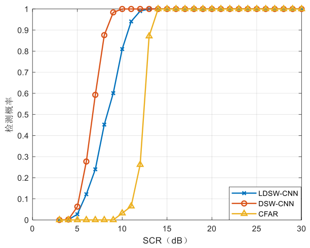
For each signal-to-clutter ratio index, 1000 targets are generated by Monte Carlo method, and the position and motion state of each target in the clutter background are inconsistent. The average detection probability of these 1000 targets is obtained by statistical method. The detection probability of the model under different signal-to-clutter ratios is obtained, as shown in Figure 22.
It can be seen from the statistics of the detection results that when the target signal-to-clutter ratio is below 12 dB, the detection probability of the DSW-CNN network is the highest, and the detection probability can reach 98 % when SCR = 9dB. When detecting targets with a signal-to-clutter ratio of 5~12dB, the detection probability of LDSW-CNN is lower than that of DSW-CNN.Since the depth of its network model is much smaller than that of DSW-CNN, the number of extracted target signal features is not enough to efficiently identify the target, and the detection probability is low. In this interval, under the same detection probability, the minimum signal-to-clutter ratio of the DSW-CNN network to detect the target is 2dB lower than that of the LDSW-CNN network and 6dB lower than that of the CFAR algorithm.
When the detection probability is above 85%, the DSW-CNN network model can detect the target with a minimum signal-to-clutter ratio of 8dB, and the LDSW-CNN network model can detect the target with a minimum signal-to-clutter ratio of 11dB, both of which can be lower than the minimum signal-to-clutter ratio detected by the CFAR algorithm.
In general, using the LDSW-CNN network model to detect targets with a signal-to-clutter ratio of less than 14dB has advantages. At the same time, the LDSW-CNN network model can also effectively detect targets with clutter of more than 10dB.
4.3. Comparative Analysis of Model Complexity
4.3.1. Simulation and comparative Analysis of Detection Performance of Different Methods
The LDSW-CNN network model is obtained by the DSW-CNN network model through knowledge distillation. They are similar in the overall structure, and the biggest difference is the size of its trainable parameters. Therefore, by comparing and analyzing the trainable parameters of the LDSW-CNN network model and the DSW-CNN network model, the degree of lightweight of the LDSW-CNN network is calculated.
The trainable parameter of the network model is an important index to measure the size of the network model [32], which is mainly determined by the weight and the number of biases in the network model. The formula for calculating the size of the trainable parameters of each convolutional layer is :
Among them, F is the number of convolution kernels of the convolution layer, K×K is the size of the convolution kernel, the depth of the feature map input by the convolution layer is Dm, and B is the number of bias terms. The proposed DSW-CNN model and LDSW-CNN model are both convolutional neural network models, and the trainable parameters only involve the convolutional layer, and the structure does not contain the fully connected layer. The scale of model parameters is shown in the following table:
| Network and layers | Calculation of parameters of each convolution layer | Trainable parameter model |
| DSW-CNN 22 layers | 31.7K | |
| LDSW-CNN 8 layers | 737 |
Based on the DSW-CNN network, the DSW-CNN network model performs a lot of pruning processing, and its trainable parameter scale is reduced to 2.32% of its teacher network, which achieves the purpose of lightweight.
4.3.2. Comparative Analysis of Time Complexity
The time complexity can evaluate the running speed of an algorithm in the case of the same hardware device. In the convolutional neural network, because the time complexity of the activation layer and the pooling layer is usually much lower than that of the convolutional layer, the time complexity of the convolutional layer is usually only calculated, and thus the time complexity of the entire convolutional neural network model is reflected. The time complexity for each convolutional layer is defined as follows :
Among them, N is the number of convolution kernels of the convolution layer, K is the size of the convolution kernel, Din is the input depth, Wout and Hout are the width and height of the output feature map.
For the CFAR algorithm, it can be calculated by the direct analysis method summarized by Zhou [33]. When processing two-dimensional signals, it involves cyclic nested loops, so the time complexity is calculated as follows :
Among them, C is the number of reference units, set to 16, J is the number of detection units, this setting is 1, W is the input data width, H is the input data height.
According to the previous experimental background, the theoretical running time of each algorithm can be obtained by calculating the time complexity when the input data size is 80 × 80. Through the actual operation, the running time of each algorithm on the experimental platform can be obtained. The CFAR algorithm is the simplest and the running time is the shortest. This method still maintains a great advantage for practical applications. The time complexity of the LDSW-CNN model is about 14.39 % of the time complexity of the DSW-CNN network, and the running time is much shorter than its teacher network. Although the running time of LDSW-CNN network is 10 times that of CFAR algorithm, it is still in millisecond level, which can meet the real-time performance of practical application. The time complexity and running time of different algorithms are shown in the following table:
| Algorithm | Time complexity | Running time |
| CFAR | 8.7557ms | |
| DSW-CNN | 204.55ms | |
| LDSW-CNN | 88.449ms |
Since the working mode of the convolutional neural network is data transmission between the convolutional layer and the convolutional layer, the detection results are finally obtained. When the CFAR algorithm processes two-dimensional data, it is only equivalent to a convolution kernel for feature map processing with a depth of 1, and the detection results are obtained. Therefore, it can be proved that the LDSW-CNN network can obtain more accurate detection results than the CFAR algorithm.
4.3.3. Summary
Three methods are used to detect the simulation targets with different signal-to-clutter ratios, and the detection results of targets with signal-to-clutter ratios of 6dB, 8dB and 14dB are compared and analyzed. The detection probability of the target with a signal-to-clutter ratio of 3 ~ 30dB is statistically and comparatively analyzed using three methods. It is concluded that the detection performance of the LDSW-CNN network is slightly lower than that of its teacher network and better than the CFAR algorithm. The performance of the three detection algorithms is compared and analyzed. Although the time complexity of the DSW-CNN network and the LDSW-CNN network is greater than that of the CFAR algorithm, and the parameter scale is also larger than that of the CFAR, the running speed of the LDSW-CNN network is still in the millisecond level, which can meet the needs of actual deployment, and the training parameters are greatly reduced compared with its teacher network. The lightweight and feasibility of LDSW-CNN network are verified.
5. Discussion
The purpose of this study is as follows : Based on the constant false alarm rate detection algorithm, a convolutional neural network is used to identify sea targets and sea clutter, and a new lightweight network model is constructed by network pruning. A convolutional neural network based on detection sliding window (DSW-CNN) and the identification technology of sea target and sea clutter are proposed. Compared with the constant false alarm rate detection, this method can adapt to more complex situations to improve the detection accuracy, and has intelligence. Compared with the traditional convolutional neural network model, it has lower hardware capacity requirements and smaller parameter model. Firstly, the characteristics of sea clutter are analyzed to obtain the characteristics that can distinguish sea clutter and target. Secondly, multi-frame radar signals are converted into graph data, and sea clutter is initially suppressed by using the spatial and temporal characteristics of graph data. Finally, through the method of knowledge distillation, an efficient and small-scale network model, namely the lightweight convolutional neural network based on detection sliding window (LDSW-CNN) model, is obtained, and the model is used to extract and classify the feature of the graph data nodes, so as to realize the target identification in the background of sea clutter, which can provide theoretical reference and technical support for subsequent deployment to edge equipment.
6. Conclusion
Electromagnetic waves will be interfered by sea clutter when detecting sea targets, which may lead to low target detection probability or even loss of targets. It is an effective solution to suppress sea clutter by identifying targets and interference. In the target detection technology under the background of sea clutter, CFAR algorithm is widely used, but its adaptability in the case of low signal-to-clutter ratio needs to be further improved. The emergence of deep learning and artificial intelligence technology provides a new idea for the suppression of sea clutter.
Based on the application background of target detection and anti-sea clutter in the background of sea clutter, this paper combines constant false alarm detection with deep learning, and proposes an intelligent identification method of sea target and sea clutter based on DSW-CNN. Firstly, the characteristics of sea clutter are analyzed to obtain the characteristics that can distinguish sea clutter and target. Then, through low threshold detection and connectivity detection, the multi-frame radar signal is converted into graph data, and the sea clutter is preliminarily suppressed by using the spatial and temporal characteristics of the graph data. Finally, the DSW-CNN model is used to extract and classify the feature of the graph data nodes, so as to realize the target identification in the background of sea clutter. In order to further reduce the weight of the proposed model, the LDSW-CNN network model is designed by pruning and trained by knowledge distillation.
Finally, CFAR, DSW-CNN network and LDSW-CNN network are used to detect targets with different signal-to-clutter ratios and analyze them. The experimental results show that the proposed method has better detection performance under low SCR conditions, which is better than the traditional CFAR method, but the running speed is slightly slower than the CFAR algorithm. In addition, the method shows strong generalization ability for different target detection scenarios. When the signal-to-clutter ratio is 12 dB, the detection probability reaches 98%. The trainable parameter size of DSW-CNN network is 31.7k, and the trainable parameter size of LDSW-CNN network is 737, which is 2.32% of the model.
References
- Qin Tianci, Wang Zhongxun, Huang Yong, etc. Review of radar CFAR target detection and processing technology [J]. Journal of Detection and Control, 2023,45 (3) : 1-11.
- Su Ningyuan, Chen Xiaolong, Key, etc. Marine micro-motion target detection and classification method based on convolutional neural network [J]. Journal of Radar, 2018, 7 (5) : 565-574.
- Wang Xing, Zhou Yipeng, Zhou Dongqing, etc. Low probability of intercept radar signal recognition based on deep belief network and bispectrum diagonal slice [J].Electronics and Informatics, 2016,38 (11) : 2972-2976.
- Xu Bin, Chen Bo, Liu Hongwei and so on. Radar high-resolution range profile target recognition based on attention recurrent neural network model [J]. Journal of Electronics and Informatics, 2016,38 (12) : 2988-2995.
- Su Ningyuan, Chen Xiaolong, Key, etc. One-dimensional sequence signal target detection method for maritime targets based on deep learning [J].Signal processing, 2020,36 (12) : 1987-1997. DOI: 10.16798/j.issn.1003-0530.2020.12.004.
- Xu Guigui. Research on sea surface weak target detection technology based on deep learning [D]. Huazhong University of Science and Technology, 2020.
- Ling Fei. Intelligent target detection method in sea clutter environment [D].University of Electronic Science and Technology of China, 2022.
- Wang Xiang, Wang Yangsheng, Chen Xingyu, etc. Multi-feature fusion sea surface target detection method based on deep learning [J]. Journal of Radar, 2024, 13 (3) : 554-564. doi: 10.12000/JR23105.
- Zhang Peng, Huang Liang, Yang Lujing, etc. Maritime target detection algorithm based on attention fusion [J].ship science and technology, 2023,45 (16) : 120-124. DOI: 10.3404/j.issn.1672-7649.2023.16.024.
- CARREIRA-PERPIÑÁN MÁ,IDELBAYEV Y.“Learning-compression” algorithms for neural net pruning[C].Washington:IEEE Computer Society,2018.8532-8541.
- XU Y H,WANG Y Z,ZHOU A J,et al.Deep neural network compression with single and multiple level quantization[C].Menlo Park:AAAI,2018.4335-4342. [CrossRef]
- Jaderberg M,Vedaldi A,Zisserman A.Speeding up Convolutional Neural Networks with Low Rank Expansions[J].Computer ence,2014,4(4):8.
- KIM J,PARK Y,KIM G,et al.SplitNet:learning to semantically split deep networks for parameter reduction and model parallelization[C].New York:ACM,2017.1866-1874.
- LECUN Y,DENKER J S,SOLLA S A.Optimal brain dam age[C].San Mateo:Morgan Kaufmann,1989.598-605.
- HINTON G E,VINYALS O,DEAN J.Distilling the know ledge in a neural network[J]. Computer Science,2015,14(7):38-39.
- Meng Constitution, Liu Fang, Li Guang, etc. An overview of knowledge distillation techniques in convolutional neural network compression [J].Computer science and exploration, 2021,15 (10) : 1812-1829.
- Key, Liu Ningbo, Wang Guoqing, etc. Radar sea detection test and target characteristic data acquisition-sea target dual-polarization multi-sea condition scattering characteristic data set [J].Radar Journal, 2023, 12 (2) : 456-469.
- Liu Ningbo, Ding Hao, Huang Yong, et al. Annual progress of X-band radar sea exploration test and data acquisition [J]. Journal of Radar, 2021, 10 (1) : 173-182.
- Liu Ningbo, Dong Yunlong, Wang Guoqing et al. X-band radar sea detection test and data acquisition [J]. Journal of Radar, 2019,8 (5) : 656-667.
- Chen Xixin, Li Po, Gong Pan. Detection Performance Analysis of Noncoherent Integration of Radar Signals [J]. Modern Radar, 2020, 42 (12) : 50-55.
- Jin K,Lai T,Qi YL,et al.Efficient coherent detection of maneuvering targets based on location rotation transform and non-uniform fast Fourier transform[J].Frontiers of Information Technology & Electronic Engineering,2020,21(8):1251-1267.
- Wang Yuchen. Analysis and simulation of sea clutter characteristics based on shipborne radar [J].Environmental technology, 2024,42 (3) : 26-29 + 48.
- Su N,Chen X,Guan J,et al.Radar Maritime Target Detection via Spatial–Temporal Feature Attention Graph Convolutional Network[J].IEEE Transactions on Geoscience and Remote Sensing,2024,62(1):1-15.
- Liu Shiqi, Kuang Huaxing, Yang Haocheng. Lightweight maritime target detection based on CFAR-CNN [J].Radar Science and Technology, 2024,22 (3) : 312-320.
- Li Hong. Research on target detection algorithm based on lightweight network [D].University of Chinese Academy of Sciences (Institute of Optoelectronic Technology, Chinese Academy of Sciences), 2022.
- Z Wang,L Du a,Y Li.Boosting Lightweight CNNs Through Network Pruning and Knowledge Distillation for SAR Target Recognition[J].IEEE Journal of Selected Topics in Applied Earth Observations and Remote Sensing,2021,14(8):8386-8397.
- Del Gaizo,Dario,et al.Hardware Deployable Radar Spectrum-based CNN classifier for Drone targets[C]. Berlin:2023 20th European Radar Conference (EuRAD),2023.131-134.
- Maurya R,Aggarwal D,Gopalakrishnan T,et al.Enhancing Deep Neural Network Convergence and Performance:A Hybrid Activation Function Approach by Combining ReLU and ELU Activation Function[C].Noida:2023 Second International Conference on Informatics (ICI),2023.1-5.
- Yu Haikun. Research on lightweight method of target detection network under resource constraints [D]. Xi 'an University of Technology, 2023.
- Chang Xilong, Liang Kun, Li Wentao. An overview of the progress of deep learning optimizers [J].Computer Engineering and Applications, 2024,60 (7) : 1-12.
- Pan Zhiming, Yin Chengzhi. Radar target echo signal simulation method [J].Electronic engineer, 2003, (7) : 56-58.
- Lin Chong, Van Gaal, Yan Wenjun, et al. A review of lightweight methods for deep neural network architectures [J]. Journal of China Academy of Electronic Science, 2024,19 (2) : 179-193.
- Zhou Shihong. Research on the analysis method of algorithm time complexity [J].Electronic components and information technology, 2023,7 (6) : 127-130 + 134.
Figure 1.
Overall flowchart of Preprocessing.
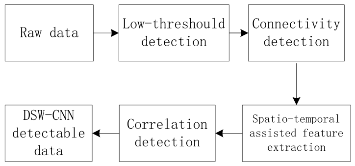
Figure 2.
Structure Diagram of the DSW-CNN network model.
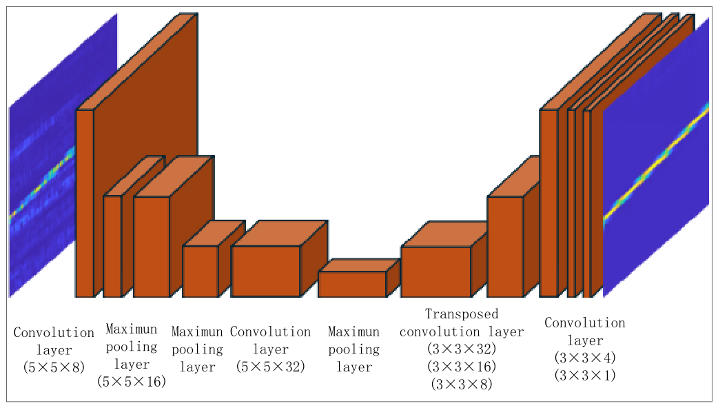
Figure 3.
Structure diagram of the LDSW-CNN network model.
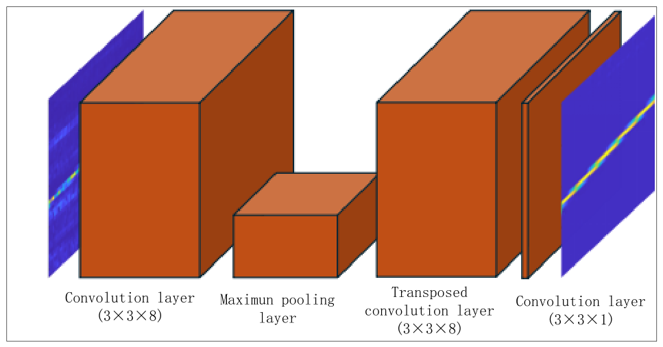
Figure 4.
Schematic diagram of the principle of the convolutional layer.
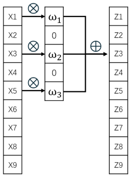
Figure 5.
Schematic diagram of the receptive field of the convolutional layer.
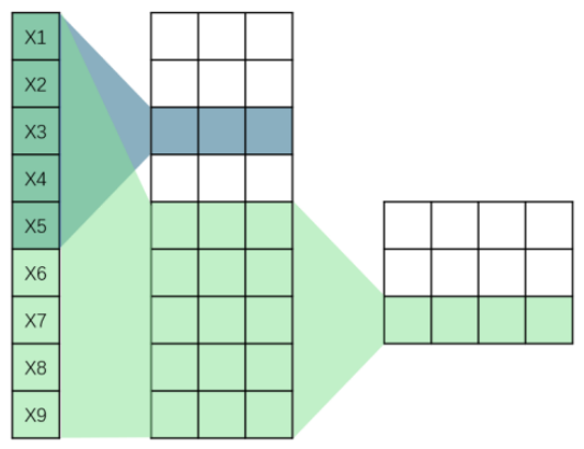
Figure 6.
Sigmoid function curve graph.
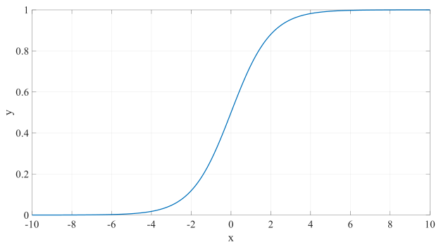
Figure 7.
Curve graph of the Tanh function.
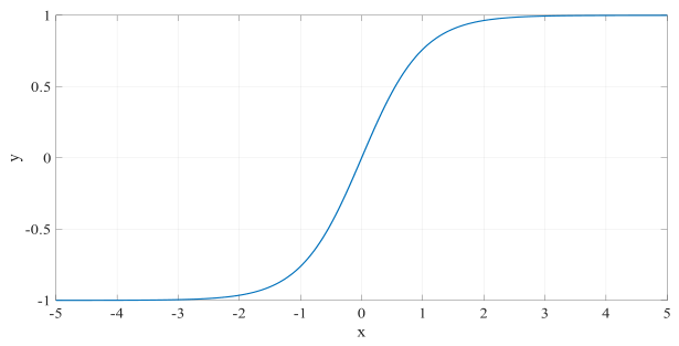
Figure 9.
Schematic diagram of the transposed convolutional layer.
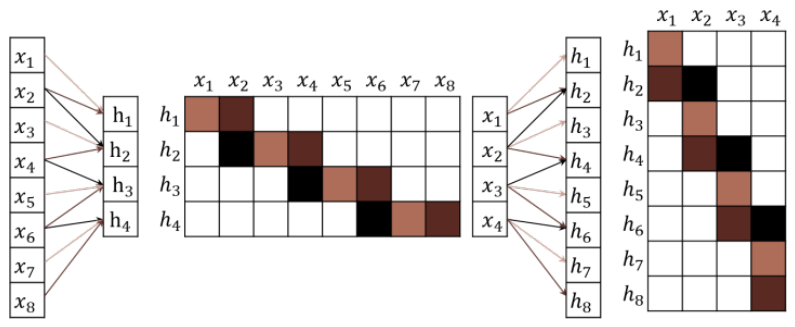
Figure 10.
Structure diagram of the post-processing layer.

Figure 11.
Diagram of the knowledge distillation training process.
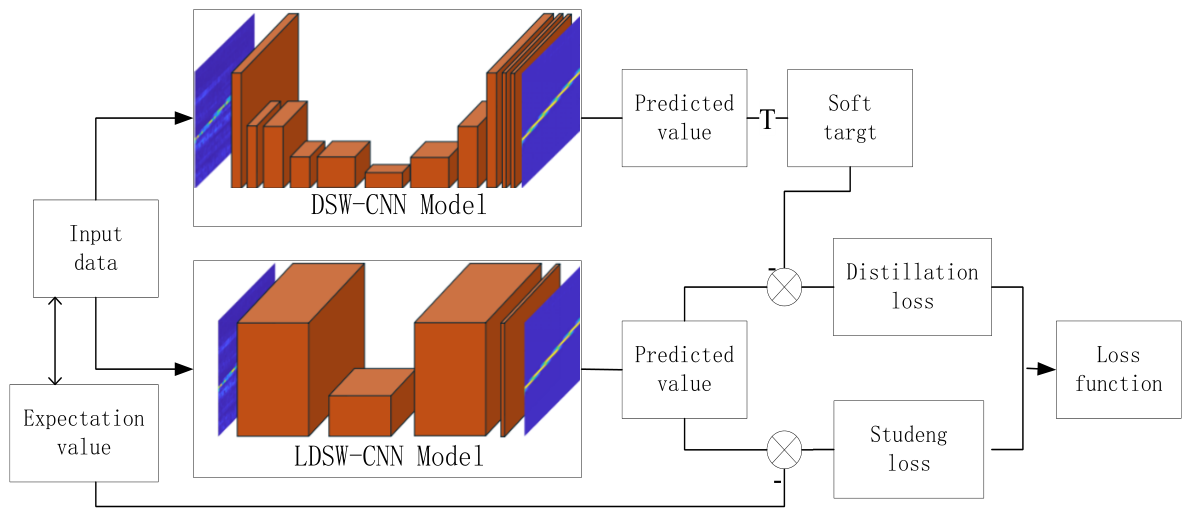
Figure 12.
Real data and target data.
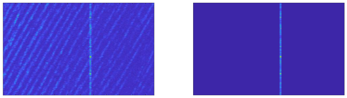
Figure 13.
Simulation data when the signal-to-noise ratio is 6dB.
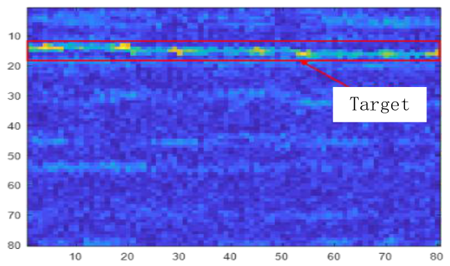
Figure 14.
Average amplitude of simulation data when the signal-to-noise ratio is 6dB.
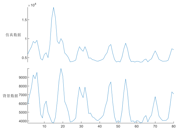
Figure 15.
Detection results when the signal-to-noise ratio is 6dB.
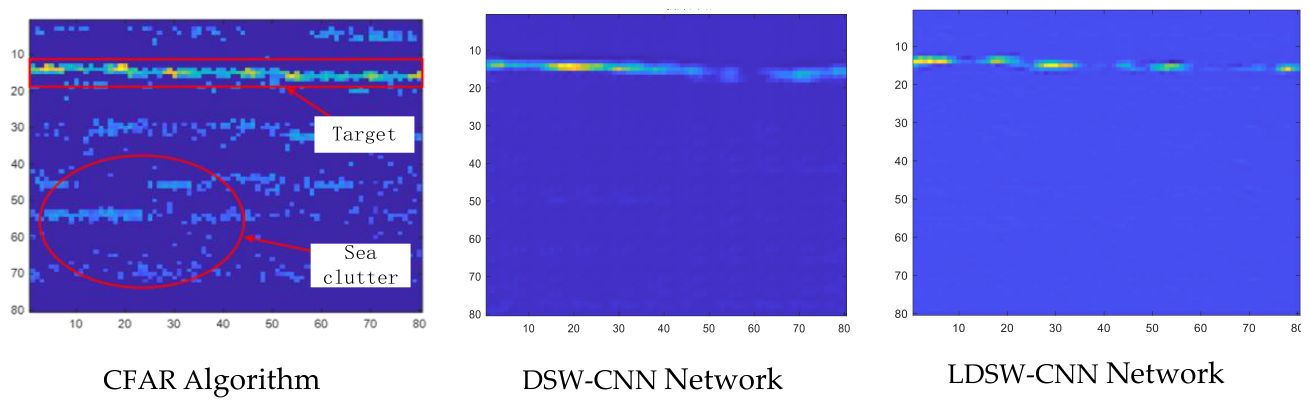
Figure 16.
Simulation data when the signal-to-noise ratio is 8dB.
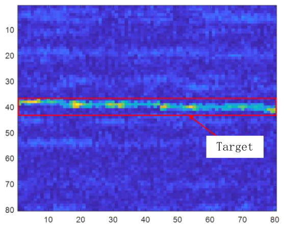
Figure 17.
Average amplitude of simulation data when the signal-to-noise ratio is 8dB.
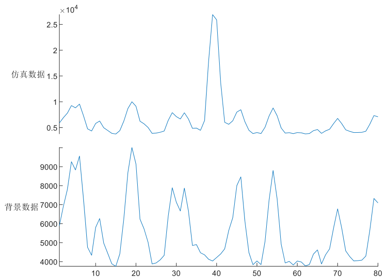
Figure 18.
Detection results when the signal-to-noise ratio is 8dB.
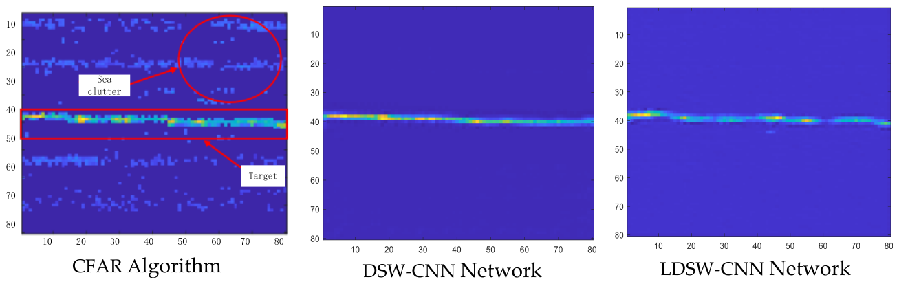
Figure 19.
Simulation data when the signal-to-noise ratio is 14dB.
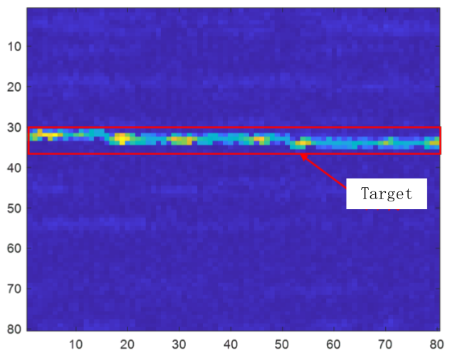
Figure 20.
Average amplitude of simulation data at a signal-to-noise ratio of 14dB.
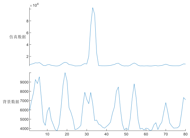
Figure 21.
Detection results when the signal-to-noise ratio is 14dB.
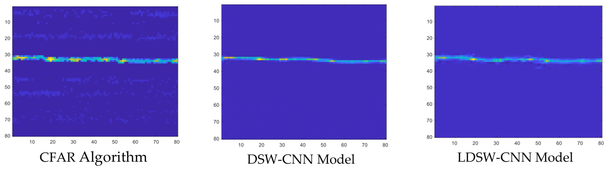
Figure 22.
Detection probabilities with different signal-to-noise ratios.
Disclaimer/Publisher’s Note: The statements, opinions and data contained in all publications are solely those of the individual author(s) and contributor(s) and not of MDPI and/or the editor(s). MDPI and/or the editor(s) disclaim responsibility for any injury to people or property resulting from any ideas, methods, instructions or products referred to in the content. |
© 2026 by the authors. Licensee MDPI, Basel, Switzerland. This article is an open access article distributed under the terms and conditions of the Creative Commons Attribution (CC BY) license (http://creativecommons.org/licenses/by/4.0/).
Copyright: This open access article is published under a Creative Commons CC BY 4.0 license, which permit the free download, distribution, and reuse, provided that the author and preprint are cited in any reuse.