Recovery in Volume, Not in Structure? Post-Pandemic Seasonal Concentration of Tourism Demand and Operating Capacity in Romania

Daniel Bulin

doi:10.20944/preprints202609.1590.v1

Submitted:

17 September 2026

Posted:

18 September 2026

You are already at the latest version

Part of the Following Collection

Preprints on COVID-19 and SARS-CoV-2

Abstract

Tourism seasonality affects destination sustainability by concentrating demand into a short period and leaving accommodation capacity underused off-season. This study examines whether Romanian tourism reverted to its pre-pandemic seasonal pattern once volumes recovered, comparing 2019 with 2025 using monthly data (INS TEMPO-Online) on arrivals, overnight stays, and net occupancy, from which operating capacity is derived. Seasonal concentration is measured with the Gini index and three complementary measures, nationally, for exhaustive partitions by visitor origin and accommodation category, and for four destination case studies. Arrivals exceeded the 2019 level by 4.89%, overnight stays returned to it, and the average length of stay fell by 5.25%; operating capacity rose by 14.03%, and net occupancy fell in every month, from 34.15% to 29.76%. The national Gini index of arrivals rose by only 1.20%; counterfactual reweighting shows that the flattening of the non-resident profile offset most of the rise for residents, and that the shift of arrivals toward 4–5-star establishments offset about half of the increase by accommodation category. Operating capacity, non-resident arrivals, and the seaside case studies moved outside the range of 12-month rolling windows on all three measures. The analysis is descriptive; national aggregates understate the redistribution it documents.

Keywords:

tourism seasonality

;

destination sustainability

;

tourism demand

;

tourism supply

;

Romanian tourism

;

COVID-19

;

Gini index

;

accommodation capacity

Subject:

Social Sciences - Tourism, Leisure, Sport and Hospitality

1. Introduction

Seasonality is a structural constraint in tourism, and it affects all three dimensions of sustainability. Economically, it generates underutilization of fixed assets. From a social perspective, it concentrates employment in short seasonal contracts with high staff turnover; from an environmental perspective, it strains water, waste, and transport infrastructure during peaks rather than across the annual volume. This study measures the economic dimension directly through occupancy of operational accommodation capacity. It treats the seasonal concentration of demand as an indicator of exposure to social and environmental effects, which the available national statistics do not allow to be measured directly. In doing so, it relates to SDG target 8.9, on policies for sustainable tourism that create jobs, and to target 12.b, on tools to monitor the sustainable development impacts of tourism—the latter being directly relevant to the monitoring argument in Section 6.1. The three dimensions share a common denominator: each depends on the pattern of activity distribution throughout the year, rather than on its annual volume.

However, measuring this form raises three problems that the literature has treated unevenly. The first concerns the object measured: the literature almost exclusively follows the concentration of demand — studies from the supply perspective being underrepresented (Wanhill, as cited in [1])— although resource consumption and economic efficiency depend directly on the capacity actually brought into operation—a matter on which operators decide from month to month. A destination can reduce its seasonal exposure either by dispersing demand or by adjusting supply, and the second path remains invisible in the usual indicators. The second problem concerns the evaluation criterion: post-pandemic analyses have treated the return to 2019 volumes as an indicator of normalization. However, from a sustainability perspective, it is the structure and not the level that matters. An unchanged concentration index is compatible with a complete reordering of the intra-annual pattern [2], and an identical volume, distributed more concentratedly, constitutes an inferior result. The third problem concerns the scale of aggregation: national indicators are reported as if they describe unitary behavior, although they result from the composition of heterogeneous regimes whose peaks compensate each other [3].

Consequently, a policy based on the national indicator may be poorly calibrated to the destinations it aggregates, a particular risk in Romania, where seaside, spa, mountain, and urban destinations exhibit markedly different seasonal patterns.

These three problems define the paper's aim: to assess whether the seasonal structure of Romanian tourism returned to its pre-pandemic form as volumes recovered, by comparing demand concentration and operating-capacity use in 2019 and 2025 and identifying which system components changed in seasonal exposure. The analysis is organized around four questions:

Q1. Has Romanian tourism returned to its previous seasonal pattern after the pandemic, or has the intra-annual structure changed independently of volume recovery?

Q2. Do arrivals and overnight stays exhibit the same seasonal pattern, or does a change in the average length of stay dissociate them, with different implications for the pressure placed on destinations?

Q3. How has the volume of capacity put into operation evolved relative to the number of overnight stays, and what does the resulting change in occupancy imply for resource-use efficiency?

Q4. In which components of the tourism system is the post-pandemic seasonal exposure concentrated?

The study makes three contributions. First, it shows that a national seasonal concentration index can change only marginally while its components move in opposite directions; furthermore, by recalibrating the weights of exhaustive partitions of the national total based on a counterfactual scenario, it quantifies the extent to which aggregate variation stems from component profiles versus changes in their weights (a methodology replicable for any set of national tourism statistics using the same partitions). Second, it analyzes demand (arrivals and overnight stays) relative to operating capacity using an accounting identity; this highlights that a national concentration of demand—which remained nearly constant—coexisted with lower monthly occupancy rates and more concentrated operating capacity. Third, the study adds to the literature on post-shock seasonality—a field previously dominated by data from Southern European destinations—by providing empirical evidence from a Central and Eastern European country, based on full calendar years following the recovery of tourism volumes.

The paper is organized as follows. Section 2 reviews the literature by topic and identifies the research gap. Section 3 presents the data and methods, Section 4 presents the results, and Section 5 discusses them in relation to the literature. Section 6 sets out the conclusions, implications for sustainable tourism development, limitations, and directions for future research.

2. Literature Review

Drawing on the distinction between natural and institutional seasonality [4,5], this study uses the origins of seasonality as an interpretive framework. Natural seasonality stems from the annual cycle of climate and daylight; for a given destination, it is largely exogenous and recurrent, and it constrains when an activity is physically possible or comfortable. Institutional seasonality stems from the calendar of human institutions—school holidays, statutory holidays, religious and legal holidays, business and event cycles, and, in Romania, publicly funded spa treatment schemes—and is, in principle, amenable to political influence. This distinction matters for two reasons. First, it identifies which components of a tourism system are likely to flatten their intra-annual profile and which are not: a destination whose season is set by sea temperature has a narrower margin for adjustment because natural conditions determine its season than one set by a corporate or academic calendar. Second, it makes changes in the aggregate indicator interpretable rather than merely observable, because a change in the relative weight of natural and institutional seasonal segments changes the national figure without any component changing its own behavior. The decompositions in sections 4.4–4.6 are interpreted in these terms. The framework is used as an interpretive device rather than as a testable hypothesis. With only one case per destination type and no data on the institutional calendar itself, the present design cannot validate the framework. Instead, Section 6.1 uses it to identify which margin of adjustment (calendar-based redistribution or the length of the operating season) is realistically available to each destination type.

To make disagreements within the corpus visible, the specialized literature is organized around five themes: the dependence of the diagnosis on the measurement instrument; the behavior of the seasonal pattern under exogenous shocks; the dissociation between arrivals and overnight stays by the length of stay; the autonomy of the trajectory of the accommodation supply; and the location of vulnerability in the components of the tourism system.

2.1. Dependence of Diagnosis on the Measuring Instrument

The first problem in the literature is not a lack of measures but their uncoordinated abundance. Koenig-Lewis and Bischoff [6] note the absence of generally accepted guidance on indicators and data sources, which makes comparisons across regions, sectors, and periods difficult. Ćorluka et al. [7] applied four methods to the same Croatian series and showed that none is superior because each captures a distinct aspect. Koenig and Bischoff [8], summarizing the merits and limitations of ten instruments, warn that scalar measures do not provide a complete picture because they capture inequality but not peak positions. The strongest argument comes from Grossi and Mussini [2], who decompose variation in the Gini index into a re-ranking component (pattern stability) and a magnitude component (intensity of concentration) and show that a conventional index is invariant to pattern change.

Chen and Pearce [9] show that the pattern can change at comparable volumes by encoding the shape of the annual curve into six patterns; Suštar and Laškarin Ažić [10] obtain, in six Mediterranean countries, three different diagnoses according to the measured component (nights, RevPAR, ADR). Ruggieri and Platania [11] obtain different hierarchies for the same nine islands depending on the indicator used. Vergori [12] adds a practical consequence: one-peak destinations register substantially higher forecast errors than two-peak ones. Studies that treat a single index as sufficient take a contrasting position. Petrevska [13], for example, characterizes seasonality in Macedonia using two indicators measured against conventional thresholds and considers this limited set of scalar measures sufficient for diagnosis. Even Ćorluka et al. [7], who argue that no single method is superior, report values that remain stable over a 12-year period, regardless of the method used. A plausible explanation for this tension concerns the scale of aggregation: convergence occurs at national aggregates, divergence at the subnational level and in decompositions, because seasonal peaks level out through mutual compensation at large territorial units, as Bender et al. [3] warn.

2.2. Behavior of the Seasonal Pattern Under Exogenous Shocks

The central question in a pre- and post-pandemic design is whether the seasonal pattern returns to its previous trajectory or suffers a permanent break. Kulendran and Wong [14] frame it as a choice between deterministic seasonality, which returns to the same seasonal averages, and stochastic non-stationarity, which implies permanent displacement. Ashworth and Thomas [15] identified an endogenous shift in the seasonal pattern in the British tourism employment data series that does not reverse during the subsequent recession. This provides evidence that changes in seasonal structure can be independent of the business cycle and, implicitly, of the recovery of tourism volumes.

Evidence of a structural rupture is also reported. Martín Martín et al. [16] find, comparing the sub-periods 2005–2007 and 2008–2010 in Andalusia, an intensification of seasonality in almost all contexts, independent of the evolution of volumes, a result confirmed by Rico et al. [17] after the 2008 crisis and by Lozano et al. [18] on the seasonality of quantities in the European double-dip recession. In qualitative terms, Senbeto and Hon [19] document the disruption of the off-peak pattern under political instability, with a prolonged off-season even after the crisis ended, and Su et al. [20] find that, in a rural Chinese destination, the pandemic prolonged the local off-season. Even in the absence of a shock, the level and structure evolve separately: Krabokoukis and Polyzos [21] show that the level of seasonality, the stability of the pattern, and the trend of volumes are independent dimensions, Xie [22] demonstrates that income and the exchange rate modify the intra-annual structure without volume being the cause, and Trajkov et al. [23] observe in Ohrid a partial neutralization of seasonality, detectable only through structural indicators, not through volumes.

Three sources support a contrasting interpretation. Cuñado et al. [24] estimate fractional seasonal integration for the Spanish series with d < 1 in all cases, implying mean reversion—slow, with hyperbolic decay—so persistent deviation, rather than reversion, would signal a real structural change. Sastre Alberti et al. [25] provide evidence from the post-COVID period on a concentration index: in Mallorca, 2021 was a seasonal outlier (Gini 0.582), and in 2022, concentration returned to the pre-pandemic trend level (0.474). Qiang [26], in turn, suggests a stability mechanism, with the pattern determined by destination type and institutional factors, with climate playing a secondary role (although the F-test for mobile seasonality is significant in both cities, suggesting the pattern may still change over time). One possible explanation for this divergence lies in the variable being measured: Ashworth and Thomas [15] measure employment, a supply variable with decisions that are difficult to reverse, while Cuñado et al. [24] model demand, and the return to the mean is an empirical result of the estimation, not a presupposition of the method; to this is added the horizon of only two years post-shock of Sastre Alberti et al. [25], which does not yet provide the distinction between the return to trend and a transitory rebound, the authors themselves warning of possible lasting effects.

2.3. Dissociation Between Arrivals and Overnight Stays by Length of Stay

Evidence does not support the implicit assumption in many studies that arrivals and overnight stays are interchangeable indicators. Bender et al. [27] found inconsistencies among the peak months of arrivals, overnight stays, and length of stay, and recommended overnight stays as a unit of measurement for capacity utilization. In a previous analysis of the same sample, the same team showed that measures calculated by length of stay form a distinct dimension that cannot be processed together with the other two [3]. For Romanian spa resorts, Stupariu and Morar [28] provide a direct demonstration: for 2010–2016, the three indicators delimit seasons of different length and position, and length of stay decreases structurally—the mechanism by which the two series can become desynchronized.

The dissociation also appears through differences in composition. Rosselló and Sansó [29] show, on daily data from the Balearic Islands, that total seasonality increased while the intra-weekly and intra-monthly components decreased, and that departures were systematically more seasonal than arrivals; Cisneros-Martínez and Fernández-Morales [30] find the classic one-peak pattern only for domestic sun-and-sand tourists, while foreign tourists are bimodal; Boto-García and Pérez [31] find that the effect of high-speed rail connectivity is maintained on arrivals but loses its significance on domestic overnight stays. Vergori and Arima [32] explain the decrease in Italian seasonality through the modal recomposition of transport, not through volumes. Duro [33] offers an important qualification: the number of tourists largely explains the concentration of income; the nuance does not, however, invalidate the dissociation, as Duro decomposes revenues, not the arrivals-overnights pair, and his result confirms precisely that the length of stay is the component that dissociates, even if its weight decreases over time. In fact, López Bonilla et al. [34] obtain the opposite result from previous Spanish data: the index on average length of stay is more concentrated than the one on the number of tourists.

2.4. Autonomy of the Trajectory of Accommodation Offer

The literature repeatedly acknowledges that the supply side remains under-researched. Puertas Medina et al. [1], citing an estimate by Wanhill, note that supply-side studies represent about 9% of the total, and Martín Martín et al. [16] describe it as much less extensive. The available results nevertheless converge on the conclusion that supply does not mechanically follow demand: Rico et al. [17] find, in six Spanish autonomous communities, a much lower seasonality of supply than demand, with its own inertia and except the Balearic Islands; Martín Martín et al. [35] finds, in the Sierras de Cazorla, a quasi-constant supply within the year, while demand fluctuates extremely; López Bonilla et al. [34] observe more moderate supply fluctuations, not coinciding with demand peaks; and Connell et al. [36] document, on Scottish tourist attractions, that 78% remain open in the off-season, with some of the closures being strategically planned, not imposed by demand.

The mechanism through which capacity becomes a cause rather than a consequence is formulated theoretically by Koenig-Lewis and Bischoff [6]: capital assets are inflexible, and permanent capacity expansion mechanically accentuates underutilization in the off-season. Lozano et al. [18] model the consequence — expansion without qualitative change of the product increases the seasonality of quantities and reduces that of prices — and Tsiotas et al. [37] empirically confirm, at the level of Greek prefecture, the association between high capacity endowment and maximum seasonality. Koenig-Lewis and Bischoff [38] support a contrasting position, documenting the deliberate withdrawal of capacity (54.3% of “seasonal performers” closed for more than one month per year, compared to 6.1% of “top performers”), driven by attitudinal logic rather than demand.

2.5. Locating Vulnerability in the Components of the Tourism System

Zhang et al. [39] showed that aggregate national-level seasonality is insignificant for financial performance because regional effects cancel each other out, concluding that predictable but large seasonality is preferable to moderate but unpredictable seasonality. Zhang and Xie [40] confirm this result on bankruptcy risk: only the business segment, the most unpredictable because it depends on the economic cycle rather than the calendar, increases the hazard rate.

Other studies locate vulnerability in specific components: Grobelna and Skrzeszewska [41] in human resources, where the negative perception of seasonality significantly reduces the intention to engage in tourism; Bampatsou et al. [42] in the workforce, with high turnover in seasonal, low-skilled, and low-paid jobs; and Smolčić Jurdana and Zmijanović [43] in space, as 98% of visits in August 2013 to the Krka National Park were concentrated in a single area that exceeded the saturation threshold, while the aggregate structure was redistributing. Wang and Chen [44] confirmed the spatial localization on perceptual data, and Vargas-Sánchez et al. [45] added the social dimension, with community attachment becoming significantly negative only at the peak of the season. Puertas Medina et al. [1] offer a more nuanced position: the most seasonal destinations are the least efficient but also the most active in innovation, compensating for the efficiency decline. Thus, high seasonality does not automatically imply net vulnerability but depends on the destination's response capacity.

2.6. Synthesis and the Research Gap

Four findings from the reviewed corpus directly inform this study's design. First, because the level and structure of seasonality are independent dimensions, a constant scalar index is compatible with a complete reordering of the intra-annual pattern [2,21]; therefore, this study must look beyond a single aggregate index. Second, because the literature is divided between the hypothesis of reversion to the mean after a shock [24,25] and that of permanent rupture [15,16], the balance between these interpretations depends on the variable chosen and the length of the post-shock window. Third, because arrivals and overnight stays are dissociated by length of stay, a mechanism documented for Romanian spa resorts by Stupariu and Morar [28], albeit for a single type of destination, based solely on pre-pandemic data and without summary concentration indices, this study must examine them jointly. Fourth, because accommodation capacity has its own inertia and can drive seasonality [6,17,18], it must also be included. The literature has not reached a consensus on whether the costs of seasonality stem primarily from its amplitude or its unpredictability [39,40]. The present study measures only the amplitude and, consequently, refers to seasonal exposure rather than vulnerability.

The research gap is twofold. First, evidence on whether seasonal patterns return after the pandemic remains scarce. Among the studies reviewed here, only Sastre Alberti et al. [25] and Su et al. [20] use post-pandemic data. In contrast, several recent studies deliberately exclude the pandemic years—2020 in Puertas Medina et al. [1] and Rico et al. [17], and the years after 2019 in Wang and Chen [44]—so the question of a return to the previous pattern remains essentially untested. Second, the dissociation between arrivals and overnight stays through length of stay has been documented mainly as a by-product of other approaches and has not been examined jointly with operating capacity in a pre- and post-shock design. Studies that decompose seasonal concentration by segment [46,47] have shown that aggregate indices can conceal divergent components, a risk that is greatest in large territorial units [3]. The present study applies this logic, descriptively, to a pre/post-pandemic comparison.

This study addresses both gaps by comparing 2019 and 2025, analyzing arrivals, overnight stays, and operating capacity on a common basis, and computing the same concentration indicators for exhaustive partitions of the national total by visitor origin and accommodation category to establish whether the components moved in the same direction as the aggregate. The aggregate change is then decomposed, via counterfactual reweighting, into a term attributable to component profiles and a term attributable to component weights (Section 4.5).

3. Materials and Methods

3.1. Data Sources and Analytical Scope

The analysis is based entirely on official tourism statistics from the National Institute of Statistics (INS), available through the TEMPO-Online database. According to the INS methodology, an arrival is recorded each time a tourist stays in an accommodation unit. Consequently, a tourist staying in multiple establishments during the same trip is counted multiple times; arrivals measure stays, not trips. This concept corresponds to the Eurostat indicator "arrivals at tourist accommodation establishments" within the harmonized system of European tourism statistics and is not comparable to international tourist arrivals recorded at borders, as reported by UN Tourism.

Three monthly series were used: tourist arrivals at tourist accommodation establishments, overnight stays recorded in the same structures, and the net occupancy rate of operating accommodation capacity. The data were extracted in August 2026, and the values correspond to the last update published by the INS at that time.

The comparison covers the calendar years 2019 and 2025, treated as pre- and post-pandemic reference points. 2019 was the last full year before the pandemic, whereas 2025 was the most recent full year after tourism volumes had recovered. No calendar year from the 2020–2024 period serves as a point of comparison: the years 2020–2023 were affected by health restrictions and the subsequent uneven recovery, while the year 2025 is used because it was the most recent full calendar year at the time of data extraction, not because it was the first year following the recovery. The second half of 2024 enters only the moving-average window and the post-pandemic rolling windows. This is a before-and-after design: differences between 2019 and 2025 reflect all changes that occurred over six years—macroeconomic, fiscal, geopolitical, and regulatory—and not the effect of the pandemic alone; ‘pre-’ and ‘post-pandemic’ are used as period labels, not as causal attributions. Changes in the register of accommodation establishments (new registrations, closures, and reclassifications) affect arrivals and operating capacity in the same direction, so the published series cannot separate them from behavioral change. Orthodox Easter fell in April and Pentecost in June in both reference years (28 April and 16 June 2019; 20 April and 8 June 2025), so these holidays do not move between months; the Easter and 1 May holidays were, however, almost contiguous in 2019 (Easter Monday on 29 April) and ten days apart in 2025, which should be kept in mind when comparing April and May. Monthly data for January–June 2026 were provisional at the time of extraction. They do not enter the calendar-year 2019 and 2025 comparisons, but they do enter the post-pandemic moving-average window and six of the thirteen post-pandemic rolling windows; the reference ranges in Appendix A, Table A7 are therefore partly based on figures that may be revised, and the classification of a change as exceeding the rolling-window range should be read with that in mind. The analysis operates with three breakdowns of tourism flows, corresponding to the nomenclatures used by the National Institute of Statistics (Romania):

• origin of visitors, distinguishing between Romanian and foreign tourists (referred to as residents and non-residents);

• accommodation category, distinguishing between establishments classified as 4- and 5-star and the group formed by 1–3-star structures and unclassified units;

• destination type, through four case studies of localities with a homogeneous functional profile: urban (Bucharest), seaside (Constanța, Mangalia, Eforie, Năvodari), spa (Băile Govora, Băile Olănești, Călimănești), and mountain (Azuga, Bușteni, Sinaia). We selected the localities for continuity in the monthly series and the dominance of a single functional profile. They are not representative samples of the corresponding national categories, and the results are not generalizable to all urban, seaside, spa, or mountain destinations in Romania.

The first two decompositions are exhaustive partitions of the national total. For the third decomposition, based on destination case studies, the results describe the behavior of the functionally defined destinations rather than the distribution of tourism across the entire territory. To keep the three breakdowns on a common basis, all are based on arrivals. Because national arrivals and overnight stays moved in opposite directions between 2019 and 2025 (Section 4.2), the component results describe the timing of arrivals, not necessarily pressure on accommodation capacity (Section 6.2).

We did not take operating accommodation capacity directly from the database; instead, we derived it from the other series, following the relationship set out in Section 3.2. The analysis is limited to officially registered establishments, as detailed in Section 6.2.

3.2. Methods

Seasonality indices. We estimated the intra-annual profile of each series using the ratio-to-centered-moving-average method.

{\bar{x}}_{t} = \frac{1}{12} (\frac{x_{t - 6}}{2} + x_{t - 5} + \dots + x_{t + 5} + \frac{x_{t + 6}}{2})

(1)

Because the moving average requires six months on either side, each 24-month window yields 12 consecutive estimates, one for each calendar month. The pre-pandemic window, January 2018–December 2019, covers the last two full calendar years unaffected by the pandemic and provides reports for July 2018–June 2019. The post-pandemic window, July 2024–June 2026, covers the most recent 24 months for which data are available and provides reports for January–December 2025. We normalized the raw indices to a mean of 100. The two windows are therefore asymmetric. The pre-pandemic profile combines July–December 2018 with January–June 2019 because a window centered on the calendar year 2019 would require data for January–June 2020. The concentration measures and all volume changes are computed for calendar years 2019 and 2025. The seasonality indices are used only to describe the shape of the profile, and a change in a given month is interpreted only when the index and the month’s share of the calendar-year total move in the same direction.

Concentration indicators. Seasonality was quantified using four measures: the traffic intensity coefficient (max/min ratio), the Gini-Struck coefficient, the Gini index (reported in the tables for each series), and the coefficient of variation (reported in the text and in Table A7). The four measures are not independent: all are functions of the same twelve monthly values, and the Gini index and the coefficient of variation, in particular, respond to the same feature of the distribution. Agreement among them is therefore a consistency check rather than independent corroboration. Disagreement, by contrast, is informative, since the Gini-Struck coefficient is computed from four seasonal groups and responds to a redistribution of mass between seasons even when month-level inequality is unchanged.

The traffic intensity coefficient is the ratio of the maximum monthly value to the minimum monthly value:

k = \frac{x_{m a x}}{x_{m i n}}

(2)

The Gini-Struck coefficient measures the deviation of the distribution across the four seasonal groups from a uniform distribution:

G_{s} = \sqrt{\frac{n \sum_{i = 1}^{n} p_{i}^{2} - 1}{n - 1}}

(3)

where pi represents the share of group i in the annual total and n = 4. The coefficient equals zero under a perfectly uniform distribution and approaches one as activity concentrates in a single season. The Gini-Struck coefficient, common in the Central and Eastern European statistical literature, is the square root of the normalized Herfindahl–Hirschman index of the seasonal shares; therefore, it measures concentration across the four seasons rather than inequality between individual months.

The Gini index is applied to the twelve monthly values and is calculated as the relative average difference:

G = \frac{\sum_{i = 1}^{n} \sum_{j = 1}^{n} |x_{i} - x_{j}|}{2 n^{2} \bar{x}}

(4)

With n = 12, this formulation reaches a maximum of (n−1)/n rather than unity, given a finite number of observations. Since all comparisons here are made across series of identical lengths, the values are reported without rescaling.

The coefficient of variation complements the intensity coefficient, which uses only the two extreme months, by measuring the dispersion of the entire profile as the percentage ratio of the sample standard deviation of the twelve values to their mean. It is calculated across all twelve monthly values, both for calendar years and rolling windows, so all reported values are on a single basis.

These measures are also computed on the net occupancy rate. Since that series consists of ratios rather than shares of an annual total, the indicators in question serve as descriptors of intra-year dispersion rather than measures of concentration in a distributional sense; only the comparison between 2019 and 2025 is interpreted for this series, and the resulting values are not comparable to those calculated for arrivals, overnight stays, or capacity.

Rolling-window range. A comparison of two calendar years does not show how sensitive each indicator is to the choice of the 12-month window. We therefore also calculated each indicator for the 13 consecutive 12-month windows within the 24 months around each reference year (from January–December 2018 to January–December 2019, and from July 2024–June 2025 to July 2025–June 2026). Consecutive windows share eleven months, so the range reflects essentially the difference between two adjacent years; it is not an estimate of year-to-year variability and has no inferential interpretation. A change is reported as exceeding the rolling-window range when the ranges for the two periods do not overlap, which flags changes that are large relative to window sensitivity. Six of the thirteen post-pandemic windows include provisional January–June 2026 data. Ranges were computed for the national series, the four components of the exhaustive partitions and the four destination case studies (Appendix A, Table A7).

Since the three indicators evaluated against the rolling-window range (the Gini index, the Gini-Struck coefficient, and the coefficient of variation) reflect different distribution characteristics, the number of indicators exceeding the respective range is recorded for each series. A series is considered more or less concentrated when at least two of the three indicators show the same trend and exceed the range, and unchanged when none of them do so; the magnitude of the change is reported separately, as a small change can still exceed a narrow range.

Counterfactual reweighting. For each exhaustive partition, the national Gini index was recalculated by adjusting the scale of each component's monthly series based on that component's annual weights from the other year, while preserving its intra-annual profile. The variation between 2019 and 2025 is decomposed into a profile-related component and a weight-related component—each calculated as the average of the two possible orderings (a two-factor Shapley decomposition)—such that the sum of the two terms exactly matches the observed variation. Updating the profile of a single component at a time makes it possible to highlight the individual contribution of each component. The seasonal structure follows the meteorological convention: winter from December to February, spring from March to May, summer from June to August, and autumn from September to November. The decomposition was computed with the assistance of Claude Opus 5 (Anthropic) from the monthly series in Appendix A (Table A5 and Table A6), from which it can be fully reproduced.

Intra-annual segments. In addition to meteorological seasons, the destination analysis (Section 4.6) uses three functional segments: the high season (June, July, and August), the mid-season (April, May, September, and October), and the low season (November–March). The three are mutually exclusive and together are exhaustive. This partition differs from the meteorological one and is used when the destination's operating logic, rather than the calendar, is in question.

Operating capacity and its use. Operating capacity is not published as a monthly series with the level of detail requested here and has therefore been reconstructed based on the following identity relationship:

C_{t} = \frac{N_{t}}{u_{t}}

(5)

where N_t denotes overnight stays and u_t the net occupancy rate in operation, expressed as a decimal. The result is expressed in bed-place days and is affected by rounding the occupancy rate to one decimal place. Because capacity equals overnight stays divided by occupancy in each month, the change in overnight stays decomposes exactly into the change in operating capacity and the change in occupancy (Δln N = Δln C + Δln u). Capacity, overnight stays, and occupancy are therefore not three independent findings but three readings of one identity; the analysis uses this identity to show how a given change in overnight stays was absorbed—by more capacity operated at lower occupancy, or by the same capacity used more intensively. It cannot establish whether supply adjusts independently of demand, since the decision to operate capacity depends on expected demand. The net occupancy rate refers to capacity in operation: establishments closed in a given month do not enter the denominator; thus, seasonal closures reduce operating capacity rather than occupancy.

The average length of stay is calculated annually and monthly as the ratio of nights spent to arrivals. Because an arrival is recorded at each accommodation establishment, the indicator measures average length of stay per establishment rather than per trip; it links the two demand-related series, since a shorter stay—assuming a constant volume of nights spent—implies more arrivals.

The net occupancy rate of operating capacity is taken directly from official statistics. This measure remains the paper’s central indicator of the economic sustainability of the supply, as it measures the proportion of operating capacity that generates income; its complement represents the non-productive fixed resource, with incompressible maintenance costs and an environmental footprint.

Expression of comparisons. Changes between 2019 and 2025 are reported as relative changes for volume measures and concentration coefficients and percentage-point changes for shares and the net occupancy rate. Differences between seasonality indices, expressed on a scale with a mean of 100, are reported in index points. All measures were computed directly from the monthly series using Equations (1)–(5); no estimation or modelling software was required.

4. Results

4.1. National Tourism Demand Seasonality: Arrivals

In 2025, Romanian tourism flows exceeded pre-pandemic levels, with total arrivals at tourist accommodation establishments reaching 13.92 million, 4.89% above the 13.27 million recorded in 2019. The concentration indicators point in the same direction, toward marginally higher concentration, but the magnitude is small — 1.20% on the Gini index — and on that measure the 12-month rolling ranges overlap: 0.1644–0.1751 before the pandemic and 0.1692–0.1839 after it. The Gini-Struck coefficient and the coefficient of variation exceed the pre-pandemic rolling-window range (post-pandemic minimum values of 0.1657 and 34.33%, compared to pre-pandemic maximum values of 0.1651 and 33.92%), whereas the Gini index does not. By the rule set out in Section 3.2, national arrivals are therefore classified as more concentrated, on two of the three indicators—the same classification as for residents and for 1–3-star and unclassified establishments. What distinguishes the national series is the magnitude of the change: +1.20% on the Gini index, against +5.62% for residents, +4.30% for 1–3-star and unclassified establishments and -16.69% for non-residents. Throughout the paper, the national aggregate is therefore described as marginally more concentrated rather than unchanged; Section 4.4, Section 4.5 and Section 4.6 and Section 5.4 show that this small change results from larger component movements in opposite directions.

Table 1. Synthetic indicators of the seasonality of tourist arrivals in Romania in 2019 and 2025.

Indicator	2019	2025	Change (%)
Total arrivals (in thousands)	13268.8	13917.7	+4.89%
Traffic intensity coefficient (max/min)	2.4648	2.5449	+3.25%
Gini-Struck coefficient (four seasonal groups)	0.1627	0.1707	+4.90%
Gini Index (12 months)	0.1698	0.1719	+1.20%
Coefficient of variation (%)	32.98	35.18	+6.67%

Note: *monthly data for 2019 and 2025; extended data and calculations can be found in Appendix A, Table A1. ource: calculations based on statistical data provided by the National Institute of Statistics.

More than half of the volume increase (58%) was concentrated in the two peak months, with July registering a plus of 10.07% compared to 2019 and August one of 11.30%; the winter months also grew (January +11.72%, December +8.72%), while the shoulder months stagnated or regressed (April –1.29%, June –0.58%, September –3.89%). September lost 3.89% in volume, 0.83 percentage points of annual share and 10.0 index points, from 119.7 to 109.6, the largest shift in the series; April, May and June also lost share.

Figure 1. Tourist arrivals—normalized seasonality indices (centered moving averages), Romania, July 2018-June 2019 and January–December 2025. Note: Seasonality indices are calculated as ratios to a 12-month moving average. Pre-pandemic period: January 2018-December 2019, generating indices for July 2018-June 2019. Post-pandemic period: July 2024-June 2026, generating indices for January–December 2025; Source: calculations based on data from the National Institute of Statistics.

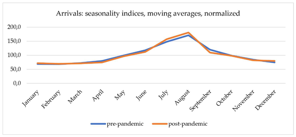
The emerging picture is not one of classic polarization between peak and off-season, but rather of internal recomposition within the tourism year: the concentration in the central summer months has intensified, while the off-season has become marginally more active. The extended summer season, spanning the months of June to September, maintained a virtually unchanged share (46.29% in 2019 and 46.42% in 2025); thus, the season did not extend in duration but rather concentrated around the peak period.

Table 2. Seasonal structure of tourist arrivals, Romania, 2019 and 2025 (%).

Season	Component months	2019	2025	Dif. (p.p.)
Winter	Dec., Jan., and Feb.	17.72	18.48	+0.76
Spring	Mar., Apr., May.	21.03	20.31	–0.72
Summer	Jun., Jul., and Aug.	36.40	37.36	+0.96
Autumn	Sep., Oct., and Nov.	24.85	23.85	–1.00

Note: monthly data for 2019 and 2025; extended data and calculations can be found in Appendix A, Table A1. Source: calculations based on data from the National Institute of Statistics.

4.2. National Tourism Demand Seasonality: Overnight Stays

Unlike arrivals, overnight stays did not exceed their pre-pandemic level: the 29.69 million recorded in 2025 are 0.62% below the 29.87 million mark from 2019. In rolling 12-month periods, figures ranged from 28.91 to 30.46 million post-pandemic, compared to 28.45–29.87 million beforehand; thus, the volume returned to a level approximately equal to that of the pre-pandemic period. The overlap of the two developments, arrivals increasing by 4.89% and overnight stays slightly decreasing, directly translates into a compression of the average length of stay, from 2.25 to 2.13 nights, i.e., a loss of 5.25%. This decrease falls outside the range of the rolling windows (2.22–2.25 nights before the pandemic, 2.11–2.13 after it).

Table 3. Synthetic indicators of seasonality of tourist overnight stays in Romania in 2019 and 2025.

Indicator	2019	2025	Change (%)	Arrivals change (%)
Total overnight stays (in thousands)	29870.4	29685.5	–0.62%	+4.89%
Traffic intensity coefficient (max/min)	3.4341	3.2505	–5.35%	+3.25%
Gini-Struck coefficient (four seasonal groups)	0.2348	0.2308	–1.70%	+4.90%
Gini Index (12 months)	0.2363	0.2261	–4.30%	+1.20%
Coefficient of variation (%)	47.51	47.43	–0.17%	+6.67%

Note: *monthly data for 2019 and 2025; extended data and calculations can be found in Appendix A, Table A2. Source: calculations based on statistical data provided by the National Institute of Statistics.

All three concentration measures indicate moderated seasonality between the two calendar years. However, irrespective of the indicator used, the values recorded in the post-pandemic periods fall within the range specific to the pre-pandemic period (Gini index: 0.2295–0.2464 before and 0.2232–0.2420 after the pandemic); consequently, the degree of concentration of overnight stays can best be described as unchanged. However, concentration remains clearly higher in both moments than for arrivals: the Gini index is 0.2261 for overnight stays in 2025 compared with 0.1719 for arrivals, because stays are longest in the peak months.

The moving-average seasonality indices show that arrivals and overnight stays follow a common pattern but differ in the magnitude of their changes. In both cases, the largest shift occurs in September, which loses 12.7 index points in overnight stays and 10.0 in arrivals, confirming the erosion of the shoulder season as a general phenomenon rather than a particularity of a series; the month also lost 10.50% in absolute terms, the most severe contraction in the entire series. The difference appears at the peak, where July and August add about nine points to arrivals but only two or three to overnight stays, while May moves in the opposite direction, with a plus of 4.5 points in overnight stays compared to a minus of 3.2 points in arrivals.

This difference is explained by the uneven decline in average length of stay throughout the year. The contraction is greatest in the peak months, where the average drops from 2.71 to 2.46 nights in August and from 2.67 to 2.46 nights in July, while in the cold months the loss remains minimal, at 0.03 nights in January and 0.01 nights in March.

Figure 2. Overnight stays—normalized seasonality indices (centered moving averages), Romania, July 2018-June 2019 and January–December 2025. Note: indices calculated as for Figure 1. Source: calculations based on data from the National Institute of Statistics.

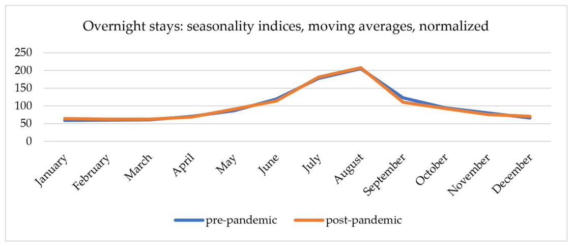
The results therefore indicate that seasonal pressure measured in nights sold did not intensify nationally but instead shifted out of autumn (–1.50 p.p.), mainly towards winter (+0.92 p.p.) and spring (+0.45 p.p.). In comparison, summer remained practically stationary (+0.13 p.p.). This conclusion does not contradict the increase in concentration observed in arrivals but complements it, since the intensification of tourism flows during the summer peak was driven by more numerous, shorter stays, with an almost neutral effect on accommodation nights sold.

Table 4. Seasonal structure of overnight stays, Romania, 2019 and 2025 (%).

Season	Component months	2019	2025	Dif. (p.p.)	Arrivals Dif.(p.p.)
Winter	Dec., Jan., and Feb.	15.60	16.53	+0.92	+0.76
Spring	Mar., Apr., May.	18.23	18.68	+0.45	–0.72
Summer	Jun., Jul., and Aug.	41.71	41.84	+0.13	+0.96
Autumn	Sep., Oct., and Nov.	24.45	22.95	–1.50	–1.00

Note: *monthly data for 2019 and 2025; extended data and calculations can be found in Appendix A, Table A2. Source: calculations based on data from the National Institute of Statistics.

4.3. Operating Capacity and the Intensity of Its Use

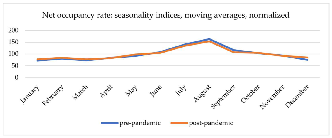
The net occupancy rate of operating accommodation capacity declined every month from 2019 to 2025, with the annual rate—calculated as the ratio of total overnight stays to total operating capacity—falling from 34.15% in 2019 to 29.76% in 2025, a decrease of 4.39 percentage points or 12.85% in relative terms. However, the deterioration was not uniform; it was concentrated in the peak months, with August down 16.12% and July 16.16%, while January fell by only 2.56%. Across calendar years, this lowers the concentration of occupancy on every measure, but the rolling 12-month ranges overlap (Gini index: 0.1353–0.1527 before and 0.1099–0.1403 after the pandemic), because occupancy fell further in the off-peak months of the first half of 2026; therefore, the flattening is not robust, whereas the decline in level is: the annual rate ranges from 32.39% to 34.15% for pre-pandemic periods and from 28.35% to 30.90% for post-pandemic ones.

The occupancy index profile also flattened at both ends: August and September each lost nine points, while December recorded an increase of 9.4 points, January 5.5 points, and May 5.8 points.

Figure 3. Net occupancy rate—normalized seasonality indices, Romania, July 2018-June 2019 and January–December 2025. Note: indices calculated as for Figure 1. Source: calculations based on data from the National Institute of Statistics.

Overnight stays and occupancy together determine operating capacity. With overnight stays 0.62% lower and occupancy 12.85% lower, operating capacity rose from 87.46 million bed-place-days in 2019 to 99.74 million in 2025 (+14.03%); across rolling 12-month windows, it ranged from 87.46 million to 87.93 million before the pandemic and from 98.55 million to 101.97 million after it (Appendix A, Table A4).

Unlike demand, operating capacity became more concentrated within the year (Table 5), outside the pre-pandemic rolling-window range on every measure (Gini index: 0.0932–0.0945 before and 0.0988–0.1084 after the pandemic). Monthly changes (Appendix A, Table A4) show why: in ten of twelve months, capacity increased by about 10.5–13%, while in July and August it increased by over 20%. The series does not distinguish between newly built capacity and existing seasonally put-into-operation stock, and the two have different policy implications; nor can a descriptive comparison determine the direction of the adjustment, since the decision to operate capacity is itself conditional on expected demand.

Read through the identity in Section 3.2, the peak months show the pattern most clearly: in July and August, operating capacity rose by more than 20%, while overnight stays increased by only 1.2–1.4%, so occupancy fell by about 16%—in August, from 52.1% to 43.7%.

4.4. Seasonality of Arrivals by Tourist Category: Residents and Non-Residents

The breakdown of arrivals by origin shows that the post-pandemic recovery was entirely domestic. Romanian tourist arrivals increased by 6.92%, from 10.60 to 11.33 million, while non-resident arrivals decreased by 3.16%, from 2.67 to 2.59 million, and the latter's share of the national total fell from 20.14% to 18.59%.

Table 6. Synthetic indicators of the seasonality of arrivals by tourist categories, Romania, 2019 and 2025.

Indicator	Residents			Non-residents
Indicator	2019	2025	Variation	2019	2025	Variation
Total arrivals (in thousands)	10597.0	11330.5	+6.92%	2671.7	2587.2	–3.16%
Traffic intensity coefficient (max/min)	2.5170	2.6829	+6.59%	2.3142	2.2206	–4.05%
Gini-Struck coefficient (four seasonal groups)	0.1694	0.1871	+10.44%	0.1467	0.1149	–21.66%
Gini Index (12 months)	0.1722	0.1819	+5.62%	0.1648	0.1373	–16.69%
Coefficient of variation (%)	34.50	38.59	+11.86%	30.46	25.27	–17.04%

Note: *monthly data for 2019 and 2025; extended data and calculations can be found in Appendix A, Table A5. Source: calculations based on statistical data provided by the National Institute of Statistics.

All four concentration indicators increase for residents and decrease for non-residents. In 2019, the two categories had similar profiles, with the Gini Index at 0.1722 for residents and 0.1648 for non-residents; by 2025, the gap widened from 0.007 to 0.045, reaching 0.1819 for residents and 0.1373 for non-residents. Domestic tourism has therefore become noticeably more concentrated than inbound tourism, reversing a hierarchy that was barely perceptible in the pre-pandemic period. Measured against the rolling 12-month windows (Appendix A, Table A7), the decline for non-residents falls outside the pre-pandemic range on every measure, whereas the increase for residents does so on the Gini-Struck coefficient and the coefficient of variation but not on the Gini index.

This observation is consistent with the very modest increase in concentration at the national level, 1.20% on the Gini index: the total combines a majority component whose concentration rises by 5.62% with a minority component whose concentration falls by 16.69%, movements that work against each other. How far they account for the aggregate outcome is taken up in Section 4.5.

The resident profile sets the direction of the national change, with residents accounting for 81.4% of arrivals in 2025. July gains 14.6 index points and August 11.9, during volume increases of 15.22% and 14.48%, respectively, while eight of the twelve months lose weight. September is the only shoulder month in absolute decline, with a loss of 3.61% and 11.5 index points, indicating a shift in domestic demand from the end of the season to its core.

Non-residents, on the contrary, describe sharp flattening. The summer peak is eroding massively, with July losing 17.0 index points and June 13.4, while the entire cold half of the year gains ground, with December gaining 22.3 points, October 9.3, and November 7.7. The result is a noticeably flatter seasonal profile of inbound tourism, with a ratio between the highest and the lowest seasonality index of 2.09, compared to 2.77 for residents.

Figure 4. Arrivals by tourist category—normalized seasonality indices, Romania, July 2018-June 2019 and January–December 2025. Note: indices calculated as for Figure 1. Source: calculations based on data from the National Institute of Statistics.

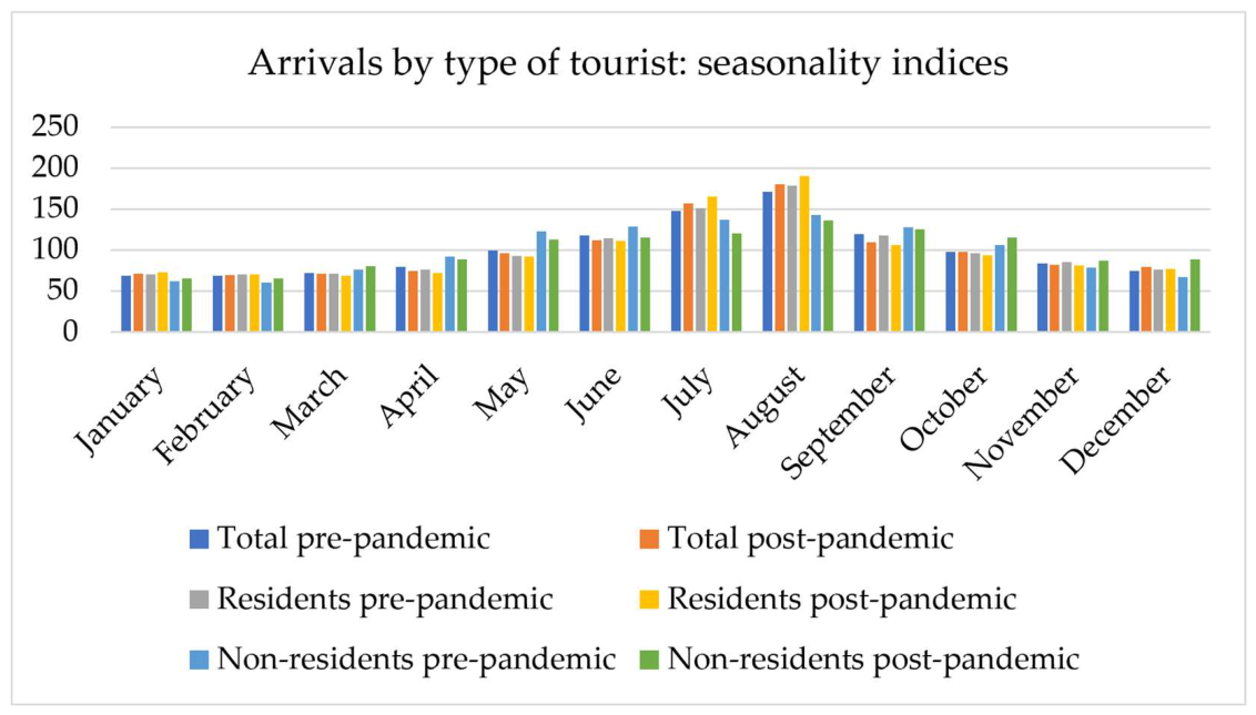
Table 7 shows the same divergence in seasonal shares. For residents, summer gains 1.67 p.p., mainly at the expense of autumn (–1.52 p.p.). For non-residents, summer loses 2.42 p.p. and spring 1.23 p.p., in favour of winter (+2.21 p.p.) and autumn (+1.43 p.p.).

Therefore, the marginal off-season activation observed at the national level is confirmed but localized: the phenomenon belongs almost exclusively to inbound tourism, whereas domestic demand behaves in the opposite way, compressing around the summer peak.

The internal profile is linked to school and legal holidays, which coincide with the natural summer season, while the external demand is not linked to this calendar and can be more easily distributed throughout the year. This explains why the two profiles differ, but not why they diverged between 2019 and 2025. Within the framework of Section 2, the candidate explanation is institutional: changes in the holiday voucher scheme for public-sector employees between 2019 and 2025, which shape the timing of domestic demand and are not tied to inbound demand. The present data do not allow this factor to be tested.

4.5. Seasonality of Arrivals by Accommodation Category

The breakdown of arrivals by classification category shows a polarization that compounds the pattern observed by origin. 4- and 5-star structures recorded 5.52 million arrivals in 2025, 12.32% above the 2019 level, while the 1–3-star segment and unclassified units stagnated, with 8.40 million compared to 8.35 million, i.e., an advance of only 0.52%. The upper segment's share of the national total consequently rose from 37.04% to 39.66%. Consequently, almost the entire increase in total arrivals (+605 thousand of the total +649 thousand) was recorded in 4- and 5-star establishments, whose seasonal profile remained virtually unchanged. Because segments are defined by the classification of establishments at each date, this change may reflect new openings and reclassifications, as well as changes in demand.

Table 8. Synthetic indicators of seasonality of arrivals by accommodation category, Romania, 2019 and 2025.

Indicator	4–5 stars			1–3 stars and unclassified
Indicator	2019	2025	%	2019	2025	%
Total arrivals (in thousands)	4914.8	5520.1	+12.32%	8354.0	8397.6	+0.52%
Traffic intensity coefficient (max/min)	1.9642	1.9870	+1.16%	2.8314	2.9762	+5.11%
Gini-Struck coefficient (four seasonal groups)	0.1174	0.1172	–0.15%	0.1909	0.2077	+8.82%
Gini Index (12 months)	0.1279	0.1259	–1.57%	0.1948	0.2031	+4.30%
Coefficient of variation (%)	23.75	23.96	+0.88%	38.91	43.08	+10.72%

Note: *monthly data for 2019 and 2025; extended data and calculations can be found in Appendix A, Table A6. Source: calculations based on statistical data provided by the National Institute of Statistics.

The gap between the two segments was already considerable in 2019, with the Gini Index at 0.1279 for 4- and 5-star establishments and 0.1948 for the remaining categories, a ratio of 1.52. In 2025, this ratio rises to 1.61, as the upper segment slightly reduces its concentration and the lower one increases it. Of all subpopulations analyzed so far, 1–3-star and unclassified establishments show the most pronounced seasonality, and it became more pronounced between the two years: their 2025 Gini index of 0.2031 compares with 0.1719 at the national level and 0.1259 in the 4–5-star segment. Against the rolling 12-month windows (Appendix A, Table A7), the increase for 1–3-star and unclassified establishments falls outside the pre-pandemic range in the Gini-Struck coefficient and the coefficient of variation, but not in the Gini index, while the change for 4–5-star establishments remains inside the pre-pandemic range on every measure.

The upper segment grew in all twelve months, most strongly in the cold months: December with 20.58%, January with 17.34%, and November with 15.62%, although the second-largest advance is in August, at 18.70%. The seasonal profile rises at both ends, with December gaining 8.1 index points and January 4.0, while the spring and early summer months lose, with April down 6.0 points and June 6.5.

The 1–3 star segment describes the opposite pattern. Seven of twelve months fell in absolute terms, and increases were limited to July and August, by 7.78% and 7.97%, respectively, January, by 8.13%, and, marginally, February and December. The sharpest index movements occur in this segment, with July gaining 14.6 points and August 13.9, while September lost 11.2 points, for an absolute contraction of 9.03%. The August index reaches 200.6, i.e., exactly double the annual average.

Figure 5. Arrivals by accommodation category—normalized seasonality indices, Romania, July 2018-June 2019 and January–December 2025. Note: indices calculated as for Figure 1. Source: calculations based on data from the National Institute of Statistics.

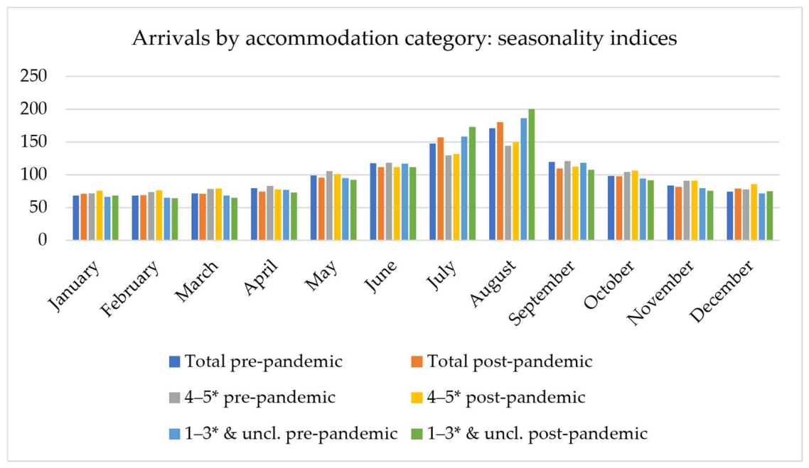
In 4- and 5-star establishments, demand is more evenly distributed throughout the year: winter gains the most (+0.9 p.p.), spring and autumn lose (–0.9 and –0.4 p.p.), and summer remains nearly unchanged (+0.4 p.p.). In the 1–3-star categories, the exact opposite happens: summer grows strongly (+1.6 p.p.), almost entirely due to autumn (–1.5 p.p.), so arrivals are even more concentrated around the summer peak.

Table 9. Seasonal structure of arrivals by accommodation category, Romania, 2019 and 2025 (%).

Season	4–5*			1–3 stars and unclassified
Season	2019	2025	Dif. (p.p.)	2019	2025	Dif. (p.p.)
Winter (Dec., Jan., Feb.)	18.84	19.76	+0.92	17.07	17.64	+0.57
Spring (Mar., Apr., May)	22.38	21.52	–0.86	20.23	19.51	–0.72
Summer (Jun., Jul., Aug.)	32.55	32.92	+0.37	38.66	40.28	+1.62
Autumn (Sep., Oct., and Nov.)	26.23	25.80	–0.43	24.04	22.57	–1.47

Note: monthly data for 2019 and 2025. Source: calculations based on data from the National Institute of Statistics.

The upper segment functions as a seasonal stabilizer and expands its activity in the cold months, a profile compatible with an urban-type demand — business, events, short weekend stays — which the aggregated data by accommodation category cannot directly confirm. The lower segment concentrates its activity increasingly in the two central months of summer, with almost zero volume growth over the year as a whole, a profile that brings it closer to the seaside regime analyzed in Section 4.6.

The two decompositions point in the same direction: the components whose concentration increased—residents and 1–3-star and unclassified establishments—are also the largest, while inbound tourism flattened its profile and the 4–5-star segment remained stable. The two partitions alone cannot establish whether these are largely the same stays, as the series used here does not cross origin with accommodation category.

Counterfactual reweighting (Section 3.2; Appendix A, Table A8) shows how each partition accounts for the +1.20% variation in the national Gini index of arrivals. By origin, updating only the resident profile would have increased the national index by 4.00%, whereas updating only the non-resident profile would have reduced it by 2.94%; the combined profile effect is +0.93%, and the weight effect is +0.27%. By accommodation category, the profile effect is +2.31%, driven by 1–3-star and unclassified units (+2.89% if updated individually, versus –0.82% for 4–5-star units), while the weight effect is –1.12%, reflecting the shift of arrivals towards 4–5-star units. The destination case studies below add a third, territorial reading.

4.6. Case Studies: Seasonality of Arrivals by Destination Type

The destination case studies illustrate how different the seasonal regimes combined in the national total are. The distance between the extremes is of a completely different order of magnitude than that observed by the origin or accommodation category, the Gini Index ranging in 2025 from 0.0720 in urban (Bucharest) to 0.6388 in seaside resorts.

Table 10. Synthetic indicators of arrival seasonality by destination case study, Romania, 2019 and 2025.

Indicator	Urban (Bucharest)	Seaside	Spa	Mountain	Romania (national total)
Arrivals 2019 (thousand)	2038.9	1272.8	1242.7	912.2	13268.8
Arrivals 2025 (thousand)	2053.7	1548.9	1206.7	802.3	13917.7
Variation (%)	+0.73	+21.70	–2.89	–12.05	+4.89
Total weight 2019 (%)	15.37	9.59	9.37	6.87	100.00
Total weight 2025 (%)	14.76	11.13	8.67	5.76	100.00
Intensity coefficient 2019	1.5249	25.1551	3.5826	2.0956	2.4648
Intensity coefficient, 2025	1.6301	32.5524	3.5359	1.9291	2.5449
Variation (%)	+6.90	+29.41	–1.30	–7.94	+3.25
Gini-Struck 2019	0.0654	0.6550	0.2135	0.1047	0.1627
Gini-Struck 2025	0.0564	0.7273	0.1781	0.0879	0.1707
Variation (%)	–13.77	+11.05	–16.59	–16.06	+4.90
Gini index 2019	0.0727	0.5924	0.2247	0.1177	0.1698
Gini index 2025	0.0720	0.6388	0.1959	0.1172	0.1719
Variation (%)	–0.98	+7.83	–12.81	–0.41	+1.20

Note: *monthly data for 2019 and 2025; the four types of destinations do not form an exhaustive partition of the territory; they total just over 40% of national arrivals. Source: calculations based on statistical data provided by the National Institute of Statistics.

In terms of the distinction introduced in Section 2, the seaside destination group is the clearest case of natural seasonality in the sample and the only one in which all concentration measures increased. Because the compression occurred within the summer season itself—gains in July and August, losses in June and September—it is more plausibly linked to institutional or market factors than to the climatic window, although climate data were not examined here. Bucharest is institutionally seasonal—its annual profile follows the business and event calendar—and shows both the flattest regime and the clearest shift toward the cold months. Spa resorts occupy an intermediate position, seasonal by therapeutic and administrative calendar rather than by climate, which is consistent with their showing the largest decline in concentration. Mountain destinations are the only ones with two natural seasons, and their movement is not flattening but a seasonal mass transfer from the summer to the winter season.

Of the four destinations, only one accentuates its seasonality — the seaside, where all indicators increase, the intensity coefficient rising by 29.41%—while the other three flatten out on most measures, the clearest attenuation belonging to the spa resorts, with a decrease of 12.81% in the Gini Index. Against the rolling 12-month windows (Appendix A, Table A7), the increase for the seaside exceeded the rolling-window range on every measure; the decline for the spa resorts remained within the wide pre-pandemic range of that series on the Gini index, the Gini-Struck coefficient, and the coefficient of variation. In Bucharest and the mountain resorts, only the Gini-Struck coefficient for Bucharest moved outside it.

Figure 6. Arrivals by destination case study— normalized seasonality index, Romania, July 2018-June 2019 and January–December 2025. Note: indices calculated as for Figure 1. Source: calculations based on data from the National Institute of Statistics.

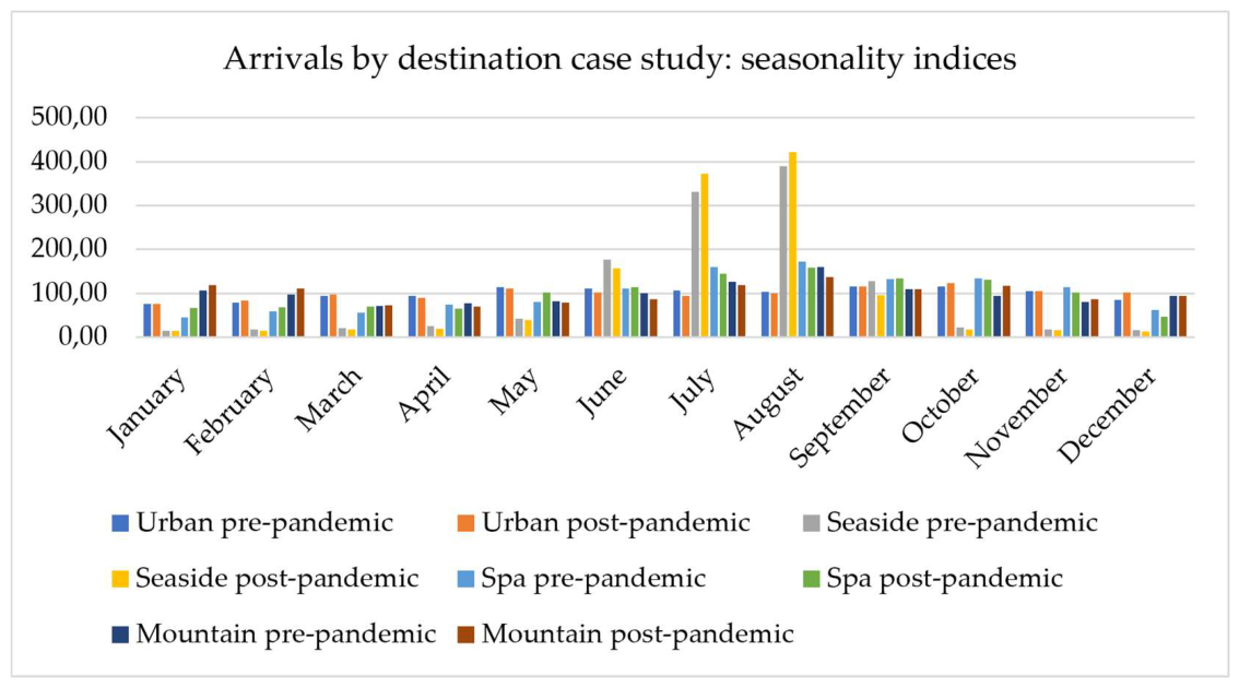
Seaside. The share of July and August in annual arrivals reached 66.28%, and the Gini index increased from 0.5924 to 0.6388. The ratio of extremes rose from 25.16 to 32.55, but because the December denominator is close to zero, this measure is unstable for the seaside group and is reported for completeness only; the seaside result relies on the Gini index, the Gini-Struck coefficient, and the coefficient of variation, which move in the same direction. Moreover, the entire volume increase was concentrated in the two peak months, with July gaining 39.6% and August 36.2%, while September lost 10.2% and October 16.1%. The seaside season was therefore concentrated further in July and August, whose share reached 66.28%, with the share of the summer quarter increasing from 73.66% to 79.36%. The off-season, already marginal, dropped from 7.53% to 6.22%.

Spa. Spa destinations show the opposite pattern, with the largest decline in concentration among the four cases, though still within the series' wide pre-pandemic range. Although total volume decreases by 2.89%, the annual structure evens out substantially, with the coefficient of variation falling from 43.09% to 36.54%. Increases are concentrated in the first half of the year, with January up 41.4%, May up 20.2%, and March up 17.9%; decreases occur in the second half, with December down 26.3%, July down 11.3%, and November down 11.0%. However, the spa profile loses its second peak: in 2019, October formed a local maximum (133.6 compared to 132.9 in September), whereas in 2025 the indices decline continuously after August, with autumn remaining a high plateau rather than a distinct peak. The share of autumn is 29.78% in 2025, the highest of the four destinations.

Mountain. Mountain destinations recorded the largest volume loss across the entire analyzed base, at 12.05%, and the contraction affected 10 of 12 months. The most severe decreases occurred in the summer months, with June down 26.3%, August down 23.6%, and April down 23.0%. The only months with an increase were October, up 19.9%, and, marginally, January, up 0.5%. The result is a shift of the seasonal mass from summer to winter. The share of summer dropped from 32.04% to 28.19%, and that of winter increased from 25.57% to 27.63%. January and February each gained almost 13 index points, while August lost 22.3. In 2025, mountain destinations maintained a profile with a still-dominant summer peak, with the August index at 137.6 compared to 118.4 in January, but the distance between the two seasons has decreased considerably.

Urban. Urban (Bucharest) confirms the role of a seasonal stabilizer previously identified. With a Gini index of 0.0720 and a coefficient of variation of 13.15%, it presents the most uniform regime in the entire base, and the volume remains practically stationary, with an advance of 0.73%. However, the internal recomposition is notable. July loses 13.2% in absolute terms and 12.5 index points, while December gains 18.4% and 17.1 points, and October gains 10.5% and 7.3 points. Summer thus falls below autumn, with a share of 25.01% compared to 28.57%, approaching spring as the weakest season of the urban year. The share in the off-season increases to 38.41%, the second-highest value among the four case studies, after the mountain localities, where it reaches 40.85%. Bucharest has therefore shifted from an almost uniform profile to one that is slightly off-seasonal compared to the rest of the tourism system.

Table 11 summarizes the contrast: the seaside gains 5.7 p.p. of summer share at the expense of every other season, whereas the urban, mountain, and spa cases lose between 2.0 and 3.9 p.p. of summer share in favor of winter and the shoulder seasons.

By destination type, the Romanian tourism system shows no general shift towards a more even distribution of demand. Only the seaside became more concentrated beyond the rolling-window range, while also recording the only substantial volume gain (+21.70%) in the most seasonal regime of the sample; the spa resorts became less concentrated on all measures, but within the wide pre-pandemic range of that series; and in Bucharest and the mountain resorts the Gini index barely changed (–0.98% and –0.41%), the change being one of timing, towards autumn and winter. Because the four case studies cover 40.32% of national arrivals and do not form a partition, their contribution to the national change cannot be established.

5. Discussion

5.1. Recovery Without a Return to the Pre-Pandemic Pattern

The answer to the first question depends on the level of analysis. At the national level, the concentration of arrivals and overnight stays in 2025 is close to that of 2019: arrivals have become marginally more concentrated, while overnight stays have shown no variation beyond the reference range. Indicators that have not returned to pre-pandemic levels include the average length of stay, the operating capacity occupancy rate, and the seasonal profiles of various components. Throughout the year, July and August gained ground at the expense of the shoulder months (particularly September), meaning that the recovery of volumes and the return to the seasonal pattern followed different trajectories.

This result falls between the two lines of evidence analyzed in Section 2.2. Sastre Alberti et al. [25] report a concentration index for Mallorca that returned to its pre-pandemic trend level in the second year after the shock, whereas Martín Martín et al. [16] and Ashworth and Thomas [15] describe intensifications of the seasonal structure that do not reverse as volumes recover. In the present case, volumes behaved as in the mean-reversion evidence—arrivals exceeded the 2019 level—while the structure behaved as in the rupture evidence, with the intra-annual distribution not returning to its previous shape. Two qualifications apply. The observation rests on a single post-pandemic calendar year, a shorter horizon than that of Sastre Alberti et al. [25], who cautioned that two years does not yet separate a return to trend from a transient recovery. The mean reversion estimated by Cuñado et al. [24] is described as slow, with hyperbolic decay, so a pattern that has not recurred after one year is not, on this evidence alone, one that will not recur.

5.2. The Divergence Between Arrivals and Overnight Stays

The results for the second question show that arrivals and overnight stays still share the same seasonal pattern but no longer move together within it: the concentration of arrivals rose slightly, that of overnight stays remained within the rolling-window range, and the average length of stay fell. The number of overnight stays has returned to a level close to 2019 (0.62% below it in 2025), and the average length of stay decreased from 2.25 to 2.13 nights, with the largest contraction occurring in the peak months: the stay in August was shortened by a quarter of a night, from 2.71 to 2.46, compared with only 0.03 nights in January. Consequently, the pressure measured in terms of nights sold did not intensify during the peak period, yet the pressure related to turnover increased: in July and August, the number of arrivals rose by 10.07% and 11.30%, respectively, while stays became shorter, implying more frequent check-ins and room turnover for a similar number of nights. Because an arrival is recorded at each establishment (Section 3.1), the data cannot distinguish more trips from the same trips split across more establishments, so the implications for travel to and from destinations—and for its environmental footprint—remain an inference that cannot be quantified with the present data.

The divergence between arrivals and overnight stays extends to the national level and to a more recent period the mechanism documented for Romanian spa resorts by Stupariu and Morar [28], who find that, for the period 2010–2016, the three indicators delineate seasons of varying duration and position and that the average length of stay decreases structurally. The current data add a consequence for concentration: the decrease in the length of stay allows arrivals to concentrate, whereas the concentration of overnight stays does not increase, so the two series can no longer be treated as interchangeable measures of the same phenomenon. This is consistent with the recommendation of Bender et al. [27] to use overnight stays when assessing capacity utilization and with the position of Vergori and Arima [32], for whom a change in seasonality may stem from behavioral recomposition rather than from volumes.

5.3. Capacity in Operation and the Efficiency of Resource Use

The accommodation capacity put into operation increased by 14.03%, from 87.46 to 99.74 million bed-place-days, but unevenly: around 10.5–13% over ten months and over 20% in July and August. The Gini index of operating capacity rose by 13.44%, a change more than ten times larger than that of arrivals and of opposite sign to that of overnight stays. Because this series is derived from overnight stays and occupancy rather than measured, the result describes the intra-annual shape of the capacity operated, not the seasonality of the accommodation stock. The additional capacity was not matched by a corresponding rise in demand: in July and August, the number of overnight stays increased by only 1.2–1.4%. The net occupancy rate decreased in all twelve months, with the annual rate falling from 34.15% to 29.76%. Operating capacity therefore increased faster than demand.

Supply remains the subject of about 9% of the seasonality literature, according to the estimate by Wanhill cited in Puertas Medina et al. [1]. Within the limits of a derived series, the result agrees with the studies reviewed in level but not in direction. As in the works of Rico et al. [17] and Martín Martín et al. [35], the seasonality of operating capacity remains much lower than that of demand (Gini index of 0.1072, compared to 0.1719 for arrivals and 0.2261 for overnight stays in 2025); unlike those studies, the degree of capacity concentration increased between the two years, whereas that of overnight stays remained unchanged. The mechanism proposed by Koenig-Lewis and Bischoff [6]—whereby rigid capital assets exacerbate off-season underutilization as capacity expands—aligns only partially with the evidence: while occupancy rates declined in every month, the drop was most pronounced in July and August (approximately 16%) and least significant in January (2.56%), meaning that underutilization increased primarily during the peak season, when operating capacity saw its greatest expansion. The descriptive approach does not allow for determining the sequence in which these adjustments occurred.

5.4. Divergent Components Beneath a Nearly Stable Aggregate

Regarding the fourth question, the national indicators describe the behavior of no single component: concentration rose for residents and for 1–3-star and unclassified establishments, fell for non-residents, and did not change beyond the rolling-window range for 4–5-star establishments (Section 4.4 and Section 4.5). This analysis of component structures aligns with the findings of Bender et al. [3]—who warn that, at the level of large territorial units, seasonal peaks mutually attenuate through offsetting effects—as well as with those of Zhang et al. [39] regarding the discrepancy between aggregated data and data analyzed at the component level.

The direction of the weight effect differs between the two partitions. The share of residents in total national arrivals rose from 79.86% to 81.41%, shifting the weight toward the component with a higher degree of concentration; conversely, the share of 4–5-star units increased from 37.04% to 39.66%, shifting the weight toward the component with a lower degree of concentration. The counterfactual decomposition analysis in Section 4.5 reveals that the relative stability of the national index stems from offsetting trends that differ by partition: regarding origin, the flattening of the non-resident seasonal profile offsets the majority of the increase observed among residents; regarding the accommodation category, the growth in the profile driven by 1–3-star and unclassified establishments is roughly halved by the shift of arrivals towards 4–5-star establishments. Since the components are aggregated for each month, this offsetting effect cannot be inferred solely from the component indices presented in Table 6 and Table 8; furthermore, as the published data series do not cross the two partitions, the analyses relating to them cannot be integrated into a single decomposition.

6. Conclusions

Taken together, the answers to the four research questions describe a recovery in volume without a return to the pre-pandemic seasonal structure. Measured in arrivals, the seasonal exposure of Romanian tourism has not been reduced but redistributed: it eased for inbound tourism, on every measure and outside the pre-pandemic range; remained stable for 4–5-star establishments; and rose in the case of domestic tourism and accommodation units classified as 1–3 stars or unclassified—the segments generating the majority of arrivals. For these two categories, the increase exceeds the range observed prior to the pandemic regarding the Gini-Struck coefficient and the coefficient of variation, though not the Gini index. Among the destination case studies, only the seaside localities became more concentrated on all measures.

A seasonality policy calibrated solely on the basis of the national indicator would have treated as uniform a change that, in the components observed here, went in opposite directions. The design is transferable beyond the Romanian case: when a national tourism system comprises segments with unequal capacities for distributing demand throughout the year, the aggregate index may mask divergent trends among its components; calculating the same indicator based on exhaustive partitions of the data—combined with counterfactual reweighting—offers a low-cost method for identifying and quantifying these phenomena.

From a sustainability perspective, the study directly measures one dimension, resource-use efficiency: operating capacity has increased, while the number of accommodation nights has not, and the net occupancy rate has decreased each month of the year. As a result, greater operating capacity—whether in the form of newly built units or existing spaces open for longer periods—now generates the same volume of nights sold. The environmental and social dimensions are addressed here only through the intra-annual distribution itself. In the seaside localities analyzed—where July and August account for two-thirds of arrivals—the strain on water, waste management, and transport infrastructure is likely to be concentrated in these same two months, and employment is likely to be limited to a season too short to sustain a stable workforce. Both interpretations are plausible and consistent with the literature reviewed in Section 2, but neither is tested against data on resource consumption or seasonal employment, which are not available in the national statistical series used here. Establishing them empirically at the destination level is the most important extension of this work and the reason why the concentration measures reported here should be interpreted as indicators of exposure rather than as measures of impact.

6.1. Implications for Sustainable Tourism Development

First, measures to extend the season should target domestic demand and the shoulder months: resident arrivals and 1–3-star or unclassified establishments are the segments where concentration has increased, while September recorded the greatest losses in both arrivals and overnight stays. In the seaside localities examined, the season contracted within the climatic window itself—June and September lost arrivals while July and August gained them—suggesting the loss is more likely institutional or market-driven (Section 4.6); consequently, recovering the shoulder months of the summer season is a more realistic goal than extending the season into the colder months. Second, operating capacity increased by 14% while overnight stays remained constant, and occupancy rates fell across every month, most sharply during the peak period. Where public funds support accommodation, the projected occupancy rate over the operating season is therefore a more informative evaluation criterion than the number of accommodation places created; applying this requires distinguishing between new capacity and the longer operation of existing units—a distinction the published datasets do not allow (Section 6.2). Third, monitoring should report overnight stays and net occupancy alongside arrivals, broken down by origin and accommodation category—a low-cost contribution to the tourism monitoring tools called for by SDG Target 12.b. Viewed solely through the lens of nationwide arrivals, the period would have appeared to mark a full recovery, with a minor shift in seasonality.

6.2. Limitations and Future Research Directions

Absence of statistical inference. The analysis is descriptive in nature. The differences between 2019 and 2025 are compared against the range of 12-month rolling windows within the 24 months around each reference year; while this approach highlights the sensitivity of the results to the choice of window, it does not constitute an estimate of year-to-year variability, nor does it assess statistical significance. Consequently, the conclusions are based on changes that are large relative to that range and consistent across the various indicators. Employing statistical testing methods—such as bootstrapping, the re-ranking test proposed by Grossi and Mussini [2], or comparisons with pre-pandemic calendar years—would make it possible to determine whether these changes exceed the typical year-to-year variation of the data series.

Uncrossed partitions. The published data series do not cross-reference visitor origin with accommodation category; consequently, the two decompositions presented in Section 4.5 cannot be combined, as it is impossible to demonstrate that the stays driving the increase among residents are the same as those driving the increase in 1–3-star and unclassified establishments.

Derived capacity. Operating capacity is not published as a monthly series and has been reconstructed from overnight stays and net occupancy rates. It is therefore a deterministic transformation of two observed series rather than an independent measurement, which limits inference: it describes the volume and intra-annual shape of the capacity actually operated, but cannot establish whether supply adjusts independently of demand. An independent monthly measurement of operating capacity, or a reconstruction of the series from the register of accommodation units and their declared operating periods, would remove this constraint.

Breakdown by destination type. The four case studies account for 41.20% of national arrivals in 2019 and 40.32% in 2025. They describe functionally characterized localities, not the entire territory, and cannot be aggregated to the national total. A functional classification covering all tourist localities in the country would allow the breakdown by destination to be exhaustive, as it already is by origin and accommodation category.

Decompositions based on arrivals. The breakdowns by origin, accommodation category, and destination use arrivals. At the national level, arrivals and overnight stays moved in opposite directions, and stays shortened most in the peak months (Section 4.2). As a result, the increase in concentration observed for residents and for 1–3-star and unclassified establishments may be smaller when measured in overnight stays. Repeating the decompositions for overnight stays would show whether the redistribution of seasonal exposure also holds for pressure on accommodation capacity.

Scope of covered supply. The capacity analyzed is that of the reception structures officially registered according to the INS methodology. Informal accommodation and, partially, accommodation mediated through platforms, which in certain destinations can represent a significant share, are not included, and their seasonal profile is not necessarily that of the registered stock.

Observation horizon. The question of a return to the previous pattern or a lasting break cannot be resolved based on a single post-pandemic year. Repeating the analysis for 2026 and 2027 would show whether the reconfiguration documented here is a stage of recovery or the new seasonal regime of Romanian tourism.

Funding

This research received no external funding.

Institutional Review Board Statement

Not applicable.

Informed Consent Statement

Not applicable.

Data Availability Statement

This study analyzed publicly available data from the National Institute of Statistics (Romania) TEMPO-Online database, extracted in August 2026. Monthly series for the years 2019 and 2025—used in the national-level analysis and in breakdowns by criteria such as visitor origin and accommodation category—are presented in Appendix A. Data series for the destination case studies and for the additional months included in the "rolling window" periods (January–December 2018 and July 2024–June 2026, with data for January–June 2026 being provisional at the time of extraction) are available in the TEMPO-Online database or can be requested from the author.

Acknowledgments

During the preparation of this manuscript, the author used Claude Opus 5 (Anthropic) to review the manuscript and suggest revisions to the text, to check the calculations reported in Appendix A, and to compute the counterfactual decomposition (Section 3.2; Appendix A, Table A8); and Grammarly (Grammarly Inc.) for language editing. The author has reviewed and edited the output and takes full responsibility for the content of this publication.

Conflicts of Interest

The author declares no conflicts of interest.

Appendix A

Table A1. Monthly tourist arrivals, shares in the annual total and normalized seasonality indices, Romania, 2019 and 2025.

Month	Arrivals 2019	Arrivals 2025	Change (%)	Share 2019 (%)	Share 2025 (%)	Dif. (p.p.)	Index pre	Index 2025	Dif. (points)
January	758,439	847,345	+11.72	5.72	6.09	+0.37	68.5	71.4	+2.9
February	758,826	817,584	+7.74	5.72	5.87	+0.16	68.3	69.2	+0.9
March	800,361	831,791	+3.93	6.03	5.98	–0.06	71.9	70.8	–1.1
April	885,822	874,422	–1.29	6.68	6.28	–0.39	79.5	74.7	–4.9
May	1,103,937	1,119,844	+1.44	8.32	8.05	–0.27	99.1	95.9	–3.2
June	1,308,897	1,301,366	–0.58	9.86	9.35	–0.51	117.5	111.9	–5.6
July	1,651,335	1,817,614	+10.07	12.45	13.06	+0.61	148.0	157.0	+9.0
August	1,869,383	2,080,676	+11.30	14.09	14.95	+0.86	171.0	180.3	+9.2
September	1,312,488	1,261,451	–3.89	9.89	9.06	–0.83	119.7	109.6	–10.0
October	1,081,817	1,121,399	+3.66	8.15	8.06	–0.10	98.2	97.9	–0.4
November	902,837	936,807	+3.76	6.80	6.73	–0.07	83.9	81.9	–2.0
December	834,614	907,409	+8.72	6.29	6.52	+0.23	74.2	79.4	+5.3
Total	13,268,756	13,917,708	+4.89	100.00	100.00	–	100.0	100.0	–

Note: Seasonality indices were calculated with the centered 12-month moving average method on the windows January 2018–December 2019 and July 2024–June 2026, which yielded indices for July 2018–June 2019 (“Index pre”) and January–December 2025 (“Index 2025”), respectively, and were normalized to an annual mean of 100. Source: own calculations based on data from the National Institute of Statistics (INS, TEMPO-Online).

Table A2. Monthly overnight stays, shares in the annual total and normalized seasonality indices, Romania, 2019 and 2025.

Month	Overnight stays 2019	Overnight stays 2025	Variation (%)	Share 2019 (%)	Share 2025 (%)	Dif. (p.p.)	Index pre	Index 2025	Dif. (points)
January	1,472,761	1,623,804	+10.26	4.93	5.47	+0.54	59.1	64.0	+5.0
February	1,496,516	1,575,013	+5.25	5.01	5.31	+0.30	59.8	62.6	+2.8
March	1,519,148	1,574,341	+3.63	5.09	5.30	+0.22	60.5	62.8	+2.3
April	1,764,779	1,715,650	–2.78	5.91	5.78	–0.13	70.2	68.6	–1.5
May	2,162,490	2,255,777	+4.31	7.24	7.60	+0.36	85.9	90.5	+4.5
June	2,993,412	2,836,305	–5.25	10.02	9.55	–0.47	118.9	114.2	–4.7
July	4,407,335	4,467,222	+1.36	14.75	15.05	+0.29	177.1	180.6	+3.5
August	5,057,673	5,117,421	+1.18	16.93	17.24	+0.31	205.0	207.6	+2.5
September	3,027,852	2,709,793	–10.50	10.14	9.13	–1.01	123.0	110.3	–12.7
October	2,352,335	2,262,346	–3.83	7.88	7.62	–0.25	94.3	92.6	–1.7
November	1,924,251	1,840,343	–4.36	6.44	6.20	–0.24	79.9	75.7	–4.2
December	1,691,806	1,707,484	+0.93	5.66	5.75	+0.09	66.3	70.5	+4.2
Total	29,870,358	29,685,499	–0.62	100.00	100.00	–	100.0	100.0	–

Note: Seasonality indices are presented in Table A1. Source: own calculations based on data from the National Institute of Statistics (INS, TEMPO-Online).

Table A3. Monthly net occupancy rate of bed-places in operation and normalized seasonality indices, Romania, 2019 and 2025.

Month	Occupancy 2019 (%)	Occupancy 2025 (%)	Variation (%)	Dif. (p.p.)	Index pre	Index 2025	Dif. (points)
January	23.4	22.8	–2.56	–0.6	71.5	77.0	+5.5
February	26.3	24.7	–6.08	–1.6	80.1	84.0	+3.9
March	24.0	22.5	–6.25	–1.5	72.9	77.0	+4.1
April	27.8	24.0	–13.67	–3.8	84.3	82.6	–1.7
May	30.3	28.2	–6.93	–2.1	91.8	97.6	+5.8
June	35.7	30.1	–15.69	–5.6	108.0	104.7	–3.3
July	45.8	38.4	–16.16	–7.4	140.1	134.5	–5.6
August	52.1	43.7	–16.12	–8.4	163.1	154.0	–9.1
September	37.7	30.2	–19.89	–7.5	116.2	107.2	–9.0
October	34.3	29.2	–14.87	–5.1	103.6	104.7	+1.1
November	29.6	25.4	–14.19	–4.2	93.1	92.0	–1.1
December	25.8	23.2	–10.08	–2.6	75.3	84.7	+9.4
Annual rate*	34.15	29.76	–12.85	–4.39	100.0	100.0	–

Note: Seasonality indices are presented in Table A1. *Annual rate calculated as total overnight stays divided by total operating capacity (Table A2 and Table A4), as in the main text; the unweighted mean of the twelve monthly rates is 32.73% in 2019 and 28.53% in 2025. Source: own calculations based on data from the National Institute of Statistics (INS, TEMPO-Online).

Table A4. Monthly operating accommodation capacity (bed-place days), derived values, and normalized seasonality indices, Romania, 2019 and 2025.

Month	Capacity 2019	Capacity 2025	Variation (%)	Index pre	Index 2025	Dif. (points)
January	6,293,850	7,121,947	+13.16	86.2	86.8	+0.7
February	5,690,175	6,376,571	+12.06	77.9	77.6	–0.3
March	6,329,783	6,997,071	+10.54	86.6	84.9	–1.7
April	6,348,126	7,148,542	+12.61	86.9	86.5	–0.4
May	7,136,931	7,999,209	+12.08	97.8	96.6	–1.1
June	8,384,908	9,422,940	+12.38	115.0	113.7	–1.3
July	9,623,002	11,633,391	+20.89	132.2	140.1	+7.9
August	9,707,626	11,710,346	+20.63	131.3	140.7	+9.4
September	8,031,438	8,972,825	+11.72	110.3	107.4	–2.9
October	6,858,120	7,747,760	+12.97	94.8	92.4	–2.4
November	6,500,848	7,245,445	+11.45	89.4	86.1	–3.2
December	6,557,388	7,359,845	+12.24	91.7	87.0	–4.6
Total	87,462,195	99,735,891	+14.03	100.0	100.0	–

Note: capacity derived as overnight stays divided by the net occupancy rate (INS, TEMPO-Online). Values are affected by rounding occupancy rates to one decimal place, with a relative error below 0.25%. Seasonality indices are presented in Table A1. Source: own calculations.

Table A5. Monthly arrivals and normalized seasonality indices by type of tourist, Romania, 2019 and 2025.

Month	Residents 2019	Residents 2025	Var. (%)	Index pre	Index 2025	Dif.	Non-residents 2019	Non-residents 2025	Var. (%)	Index pre	Index 2025	Dif.
January	618,621	713,079	+15.27	70.1	72.6	+2.6	139,818	134,266	–3.97	62.1	65.4	+3.4
February	623,876	683,154	+9.50	70.3	70.1	–0.2	134,950	134,430	–0.39	60.3	65.2	+5.0
March	631,270	664,394	+5.25	70.9	68.7	–2.2	169,091	167,397	–1.00	75.8	80.4	+4.6
April	681,807	687,678	+0.86	76.5	71.6	–4.9	204,015	186,744	–8.47	91.6	88.6	–3.0
May	831,301	880,382	+5.90	93.2	92.2	–1.0	272,636	239,462	–12.17	122.5	112.4	–10.2
June	1,022,762	1,052,804	+2.94	114.7	111.1	–3.5	286,135	248,562	–13.13	128.7	115.3	–13.4
July	1,350,243	1,555,728	+15.22	150.8	165.5	+14.6	301,092	261,886	–13.02	137.2	120.3	–17.0
August	1,557,077	1,782,530	+14.48	178.7	190.5	+11.9	312,306	298,146	–4.53	142.5	136.4	–6.1
September	1,024,725	987,707	–3.61	117.5	106.0	–11.5	287,763	273,744	–4.87	127.5	125.0	–2.5
October	843,025	868,302	+3.00	96.1	93.7	–2.4	238,792	253,097	+5.99	106.2	115.6	+9.3
November	726,382	745,903	+2.69	85.2	80.8	–4.4	176,455	190,904	+8.19	78.9	86.6	+7.7
December	685,959	708,807	+3.33	76.1	77.1	+1.0	148,655	198,602	+33.60	66.7	89.0	+22.3
Total	10,597,048	11,330,468	+6.92	100.0	100.0	–	2,671,708	2,587,240	–3.16	100.0	100.0	–

Note: Seasonality indices are presented in Table A1. Source: own calculations based on data from the National Institute of Statistics (INS, TEMPO-Online).

Table A6. Monthly arrivals and normalized seasonality indices by accommodation category, Romania, 2019 and 2025.

Month	4–5* 2019	4–5* 2025	Var. (%)	Index pre	Index 2025	Dif.	1–3* & uncl. 2019	1–3* & uncl. 2025	Var. (%)	Index pre	Index 2025	Dif.
January	295,796	347,074	+17.34	72.1	76.1	+4.0	462,643	500,271	+8.13	66.3	68.4	+2.1
February	303,794	350,187	+15.27	74.0	76.6	+2.6	455,032	467,397	+2.72	65.0	64.6	–0.4
March	322,011	363,939	+13.02	78.4	79.3	+0.9	478,350	467,852	–2.19	68.2	65.3	–2.8
April	343,395	356,601	+3.85	83.4	77.5	–6.0	542,427	517,821	–4.54	77.3	72.8	–4.4
May	434,514	467,136	+7.51	105.5	101.2	–4.4	669,423	652,708	–2.50	95.4	92.4	–2.9
June	488,170	518,071	+6.13	118.6	112.1	–6.5	820,727	783,295	–4.56	116.9	111.7	–5.2
July	530,654	609,734	+14.90	129.6	132.0	+2.4	1,120,681	1,207,880	+7.78	158.8	173.4	+14.6
August	580,995	689,628	+18.70	144.6	149.5	+4.9	1,288,388	1,391,048	+7.97	186.7	200.6	+13.9
September	494,805	517,641	+4.62	121.0	112.5	–8.5	817,683	743,810	–9.03	118.8	107.6	–11.2
October	432,850	488,691	+12.90	104.3	106.5	+2.2	648,967	632,708	–2.51	94.6	92.0	–2.6
November	361,261	417,682	+15.62	90.8	91.0	+0.2	541,576	519,125	–4.15	79.9	75.8	–4.1
December	326,531	393,738	+20.58	77.6	85.8	+8.1	508,083	513,671	+1.10	72.1	75.1	+3.0
Total	4,914,776	5,520,122	+12.32	100.0	100.0	–	8,353,980	8,397,586	+0.52	100.0	100.0	–

Note: 4–5*: establishments classified at four and 5 stars; 1–3* & uncl.: establishments classified at 1–3 stars and unclassified units. Seasonality indices are presented in Table A1. Source: own calculations based on data from the National Institute of Statistics (INS, TEMPO-Online).

Table A7. Ranges of the concentration measures over the thirteen 12-month rolling windows of each period, Romania.

Series	Gini pre	Gini post	Gini-Struck pre	Gini-Struck post	CV pre (%)	CV post (%)	Outside the pre-pandemic range
Arrivals (national)	0.1644–0.1751	0.1692–0.1839	0.1535–0.1651	0.1657–0.1798	32.04–33.92	34.33–37.01	GS ↑, CV ↑
Overnight stays (national)	0.2295–0.2464	0.2232–0.2420	0.2234–0.2412	0.2255–0.2445	46.38–49.52	46.44–50.06	none
Net occupancy rate (national)	0.1353–0.1527	0.1099–0.1403	0.1238–0.1440	0.1046–0.1332	26.63–29.84	22.11–27.38	none
Operating capacity (national)	0.0932–0.0945	0.0988–0.1084	0.0900–0.0931	0.1001–0.1101	17.95–18.39	20.05–21.85	Gini ↑, GS ↑, CV ↑
Residents	0.1629–0.1813	0.1765–0.1988	0.1549–0.1738	0.1762–0.2015	32.96–36.12	36.74–41.25	GS ↑, CV ↑
Non-residents	0.1625–0.1735	0.1294–0.1481	0.1454–0.1554	0.1034–0.1302	30.03–32.09	23.78–27.38	Gini ↓, GS ↓, CV ↓
4–5*	0.1249–0.1350	0.1210–0.1327	0.1124–0.1230	0.1135–0.1226	23.24–24.95	23.00–25.14	none
1–3* & uncl.	0.1878–0.1990	0.1977–0.2186	0.1793–0.1919	0.1961–0.2208	37.66–39.74	41.07–45.52	GS ↑, CV ↑
Urban (Bucharest)	0.0727–0.0789	0.0630–0.0855	0.0654–0.0721	0.0531–0.0634	13.56–14.68	11.73–15.80	GS ↓
Seaside	0.5924–0.6121	0.6362–0.6443	0.6550–0.6701	0.7268–0.7330	128.92–135.63	145.21–147.31	Gini ↑, GS ↑, CV ↑
Spa	0.2166–0.2764	0.1749–0.2269	0.2003–0.2633	0.1637–0.2151	39.87–51.24	32.66–42.39	none
Mountain	0.1120–0.1424	0.1090–0.1470	0.0923–0.1187	0.0869–0.1174	22.15–27.50	20.26–27.81	none

Note: Pre: windows January–December 2018 to January–December 2019; post: windows July 2024-June 2025 to July 2025-June 2026. The coefficient of variation is calculated on monthly values. Last column: measures whose post-pandemic range does not overlap the pre-pandemic range (↑ above, ↓ below). Source: own calculations based on data from the National Institute of Statistics (INS, TEMPO-Online).

Table A8. Counterfactual decomposition of the change in the national Gini index of arrivals, 2019–2025 (% of the 2019 value).

	By origin	By accommodation category
Observed change	+1.20	+1.20
Profile effect	+0.93	+2.31
Weight effect	+0.27	–1.12
Only first component's profile updated*	+4.00 (residents)	–0.82 (4–5*)
Only second component's profile updated*	–2.94 (non-residents)	+2.89 (1–3* & uncl.)

Note: Profile and weight effects are averaged over both orderings and sum to the observed change (differences due to rounding). *At 2019 component weights; the two single-component effects are not additive. Source: own calculations based on Table A5 and Table A6.

References

Puertas Medina, R.M.; Martín Martín, J.M.; Guaita Martínez, J.M.; Serdeira Azevedo, P. Analysis of the role of innovation and efficiency in coastal destinations affected by tourism seasonality. J. Innov. Knowl. 2022, 7, 100163. [Google Scholar] [CrossRef]
Grossi, L.; Mussini, M. Seasonality in tourist flows: Decomposing and testing changes in seasonal concentration. Tour. Manag. 2021, 84, 104289. [Google Scholar] [CrossRef]
Bender, O.; Schumacher, K.P.; Stein, D. Measuring seasonality in Central Europe’s tourism—How and for what? In Proceedings of CORP 2005 & Geomultimedia05; Vienna, Austria, Schrenk, M., Ed.; 2005; pp. 303–309. [Google Scholar]
BarOn, R.R.V. Seasonality in Tourism: A Guide to the Analysis of Seasonality and Trends for Policy Making; Technical Series No. 2; Economist Intelligence Unit: London, UK, 1975. [Google Scholar]
Butler, R.W. Seasonality in tourism: Issues and implications. In Seasonality in Tourism; Baum, T., Lundtorp, S., Eds.; Pergamon: Oxford, UK, 2001; pp. 5–21. [Google Scholar]
Koenig-Lewis, N.; Bischoff, E.E. Seasonality research: The state of the art. Int. J. Tour. Res. 2005, 7, 201–219. [Google Scholar] [CrossRef]
Ćorluka, G.; Vukušić, A.; Kelić, I. Measuring tourism seasonality: Application and comparison of different methods. In Proceedings of the Tourism & Hospitality Industry 2018, Congress Proceedings, Opatija, Croatia; University of Rijeka: Rijeka, Croatia, 2018; pp. 55–63. [Google Scholar]
Koenig, N.; Bischoff, E.E. Seasonality of tourism in Wales: A comparative analysis. Tour. Econ. 2003, 9, 229–254. [Google Scholar] [CrossRef]
Chen, T.; Pearce, P.L. Research note: Seasonality patterns in Asian tourism. Tour. Econ. 2012, 18, 1105–1115. [Google Scholar] [CrossRef]
Suštar, N.; Laškarin Ažić, M. Measuring tourism seasonality across selected Mediterranean countries. KnE Soc. Sci. 2019, 4, 216–229. [Google Scholar] [CrossRef]
Ruggieri, G.; Platania, M. Islands’ tourism seasonality: A data analysis of Mediterranean islands’ tourism comparing seasonality indicators (2008–2018). Sustainability 2024, 16, 3674. [Google Scholar] [CrossRef]
Vergori, A.S. Patterns of seasonality and tourism demand forecasting. Tour. Econ. 2017, 23, 1011–1027. [Google Scholar] [CrossRef]
Petrevska, B. Investigating tourism seasonality in Macedonia. UTMS J. Econ. 2013, 4, 37–44. [Google Scholar]
Kulendran, N.; Wong, K.K.F. Modeling seasonality in tourism forecasting. J. Travel Res. 2005, 44, 163–170. [Google Scholar] [CrossRef]
Ashworth, J.; Thomas, B. Patterns of seasonality in employment in tourism in the UK. Appl. Econ. Lett. 1999, 6, 735–739. [Google Scholar] [CrossRef]
Martín Martín, J.M.; Jiménez Aguilera, J.d.D.; Molina Moreno, V. Impacts of seasonality on environmental sustainability in the tourism sector based on destination type: An application to Spain’s Andalusia region. Tour. Econ. 2014, 20, 123–142. [Google Scholar] [CrossRef]
Rico, P.; Cabrer-Borrás, B.; Morillas-Jurado, F. Seasonality in tourism: Do senior programs mitigate it? Mathematics 2021, 9. [Google Scholar] [CrossRef]
Lozano, J.; Rey-Maquieira, J.; Sastre, F. An integrated analysis of tourism seasonality in prices and quantities, with an application to the Spanish hotel industry. J. Travel Res. 2021, 60, 1581–1597. [Google Scholar] [CrossRef]
Senbeto, D.L.; Hon, A.H.Y. Shaping organizational culture in response to tourism seasonality: A qualitative approach. J. Vacat. Mark. 2021, 27, 466–478. [Google Scholar] [CrossRef]
Su, Z.; Wen, R.; Zeng, Y.; Ye, K.; Khotphat, T. The influence of seasonality on the sustainability of livelihoods of households in rural tourism destinations. Sustainability 2022, 14, 10572. [Google Scholar] [CrossRef]
Krabokoukis, T.; Polyzos, S. Analyzing the tourism seasonality for the Mediterranean countries. J. Knowl. Econ. 2024, 15, 8053–8076. [Google Scholar] [CrossRef]
Xie, J. The economic determinants of tourism seasonality: A case study of the Norwegian tourism industry. Cogent Bus. Manag. 2020, 7, 1732111. [Google Scholar] [CrossRef]
Trajkov, A.; Biljan, J.; Andreeski, C. Overview and characteristics of tourism seasonality in Ohrid. Econ. Themes 2016, 54, 485–498. [Google Scholar] [CrossRef]
Cuñado, J.; Gil-Alana, L.A.; Pérez de Gracia, F. The nature of seasonality in Spanish tourism time series. Tour. Econ. 2005, 11, 483–499. [Google Scholar] [CrossRef]
Sastre Alberti, F.; Rey-Maquieira, J.; Lozano, J. Tourism seasonality and public policy: An exploratory analysis—Lessons from Mallorca, Spain. Investig. Turísticas 2025, 30, 74–91. [Google Scholar] [CrossRef]
Qiang, M. Does climate drive tourism seasonality in cultural destinations? A comparative study. Curr. Issues Tour. 2020, 23, 2756–2761. [Google Scholar] [CrossRef]
Bender, O.; Schumacher, K.P.; Stein, D. Landscape, seasonality, and tourism: A survey with examples from Central Europe. In Seasonal Landscapes; Palang, H., Sooväli, H., Printsmann, A., Eds.; Landscape Series: Dordrecht, The Netherlands; Springer, 2007; Volume 7, pp. 181–213. [Google Scholar]
Stupariu, M.I.; Morar, C. Tourism seasonality in the spas of Romania. GeoJ. Tour. Geosites 2018, 22, 573–584. [Google Scholar] [CrossRef]
Rosselló, J.; Sansó, A. Yearly, monthly and weekly seasonality of tourism demand: A decomposition analysis. Tour. Manag. 2017, 60, 379–389. [Google Scholar] [CrossRef]
Cisneros-Martínez, J.D.; Fernández-Morales, A. Cultural tourism as tourist segment for reducing seasonality in a coastal area: The case study of Andalusia. Curr. Issues Tour. 2015, 18, 765–784. [Google Scholar] [CrossRef]
Boto-García, D.; Pérez, L. The effect of high-speed rail connectivity and accessibility on tourism seasonality. J. Transp. Geogr. 2023, 107, 103546. [Google Scholar] [CrossRef]
Vergori, A.S.; Arima, S. Transport modes and tourism seasonality in Italy: By air or by road? Tour. Econ. 2022, 28, 583–598. [Google Scholar] [CrossRef]
Duro, J.A. Seasonality of tourism: A new decomposition. Tour. Econ. 2018, 24, 615–621. [Google Scholar]
López Bonilla, J.M.; López Bonilla, L.M.; Sanz Altamira, B. Patterns of tourist seasonality in Spanish regions. Tour. Hosp. Plan. Dev. 2006, 3, 241–256. [Google Scholar] [CrossRef]
Martín Martín, J.M.; Salinas Fernández, J.A.; Rodríguez Martín, J.A.; Ostos Rey, M.d.S. Analysis of tourism seasonality as a factor limiting the sustainable development of rural areas. J. Hosp. Tour. Res. 2020, 44, 45–75. [Google Scholar] [CrossRef]
Connell, J.; Page, S.J.; Meyer, D. Visitor attractions and events: Responding to seasonality. Tour. Manag. 2015, 46, 283–298. [Google Scholar] [CrossRef]
Tsiotas, D.; Krabokoukis, T.; Polyzos, S. Detecting interregional patterns in tourism seasonality of Greece: A principal components analysis approach. Reg. Sci. Inq. 2020, 12, 91–112. [Google Scholar]
Koenig-Lewis, N.; Bischoff, E.E. Developing effective strategies for tackling seasonality in the tourism industry. Tour. Hosp. Plan. Dev. 2010, 7, 395–413. [Google Scholar] [CrossRef]
Zhang, D.; Xie, J.; Sikveland, M. Tourism seasonality and hotel firms’ financial performance: Evidence from Norway. Curr. Issues Tour. 2021, 24, 3021–3039. [Google Scholar] [CrossRef]
Zhang, D.; Xie, J. Influence of tourism seasonality and financial ratios on hotels’ exit risk. J. Hosp. Tour. Res. 2023, 47, 714–733. [Google Scholar] [CrossRef]
Grobelna, A.; Skrzeszewska, K. Seasonality: Is it a problem or challenge facing future tourism employment? Implications for management. J. Entrep. Manag. Innov. 2019, 15, 205–230. [Google Scholar] [CrossRef]
Bampatsou, C.; Halkos, G.; Astara, O.-H. Composite indicators in evaluating tourism performance and seasonality. Oper. Res. 2022, 22, 2373–2396. [Google Scholar] [CrossRef]
Smolčić Jurdana, D.; Zmijanović, L. The effect of tourism seasonality on protected areas. In Proceedings of the Tourism and Hospitality Industry 2014: Trends in Tourism and Hospitality Industry, Congress Proceedings, Opatija, Croatia; University of Rijeka: Rijeka, Croatia, 2014; pp. 131–146. [Google Scholar]
Wang, J.; Chen, X. Balancing tourism seasonality: The role of tourism destination image (TDI) and spatial levels (SLs). Sustainability 2025, 17, 2569. [Google Scholar] [CrossRef]
Vargas-Sánchez, A.; Porras-Bueno, N.; Plaza-Mejía, M.Á. Residents’ attitude to tourism and seasonality. J. Travel Res. 2014, 53, 581–596. [Google Scholar] [CrossRef]
Duro, J.A. Seasonality of hotel demand in the main Spanish provinces: Measurements and decomposition exercises. Tour. Manag. 2016, 52, 52–63. [Google Scholar] [CrossRef]
Fernández-Morales, A.; Cisneros-Martínez, J.D.; McCabe, S. Seasonal concentration of tourism demand: Decomposition analysis and marketing implications. Tour. Manag. 2016, 56, 172–190. [Google Scholar] [CrossRef]

Table 5. Net occupancy rate and operating capacity: level and intra-annual dispersion, Romania, 2019 and 2025.

Indicator	Occupancy			Capacity (mn bed-place days)
Indicator	2019	2025	Change	2019	2025	Change
Level	34.15%	29.76%	–4.39 p.p.	87.46	99.74	+14.03%
Traffic intensity coefficient (max/min)	2.2265	1.9422	–12.77%	1.7060	1.8365	+7.65%
Gini-Struck coefficient	0.1327	0.1092	–17.72%	0.0931	0.1078	+15.81%
Gini index (12 months)	0.1405	0.1142	–18.71%	0.0945	0.1072	+13.44%
Coefficient of variation (%)	27.24	23.05	–15.38%	18.39	21.45	+16.62%

Note: for the occupancy rate, a ratio, the measures describe intra-year dispersion and are not comparable with the concentration measures for arrivals, overnight stays or capacity (Section 3.2). Source: calculations based on statistical data provided by the National Institute of Statistics.

Table 7. Seasonal structure of arrivals by tourist category, Romania, 2019 and 2025 (%).

Season	Residents			Non-residents
Season	2019	2025	Dif. (p.p.)	2019	2025	Dif. (p.p.)
Winter	18.20	18.58	+0.38	15.85	18.06	+2.21
Spring	20.24	19.70	–0.53	24.17	22.94	–1.23
Summer	37.09	38.75	+1.67	33.67	31.25	–2.42
Autumn	24.48	22.96	–1.52	26.31	27.74	+1.43

Note: *monthly data for 2019 and 2025; extended data and calculations can be found in Appendix A, Table A5. Source: calculations based on data from the National Institute of Statistics.

Table 11. Seasonal structure of arrivals by destination type, Romania, 2019 and 2025 (%).

Season	Urban (Bucharest)		Seaside		Spa		Mountain
Season	2019	2025	2019	2025	2019	2025	2019	2025
Winter	20.28	21.68	4.05	3.43	13.88	15.21	25.57	27.63
Spring	25.33	24.74	7.51	6.35	18.41	20.20	19.90	18.63
Summer	27.11	25.01	73.66	79.36	36.84	34.81	32.04	28.19
Autumn	27.29	28.57	14.77	10.86	30.88	29.78	22.49	25.55

Note: monthly data for 2019 and 2025. Source: calculations based on data from the National Institute of Statistics.

Disclaimer/Publisher’s Note: The statements, opinions and data contained in all publications are solely those of the individual author(s) and contributor(s) and not of MDPI and/or the editor(s). MDPI and/or the editor(s) disclaim responsibility for any injury to people or property resulting from any ideas, methods, instructions or products referred to in the content.

© 2026 by the authors. Licensee MDPI, Basel, Switzerland. This article is an open access article distributed under the terms and conditions of the Creative Commons Attribution (CC BY) license (http://creativecommons.org/licenses/by/4.0/).

Copyright: This open access article is published under a Creative Commons CC BY 4.0 license, which permit the free download, distribution, and reuse, provided that the author and preprint are cited in any reuse.