

Submitted:
17 September 2026
Posted:
18 September 2026
You are already at the latest version
Abstract
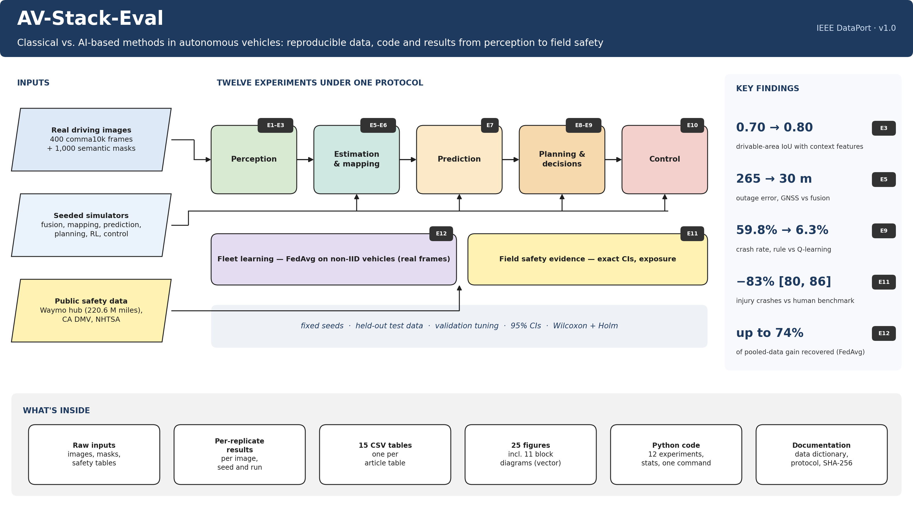
Artificial intelligence (AI) is used throughout autonomous vehicle (AV) software, yet published comparisons of perception, estimation, prediction, planning and control methods rarely share data, protocols or statistical analysis, which makes their trade-offs difficult to judge. This paper reports a reproducible experimental evaluation that spans the AV stack under a single protocol: fixed seeds, held-out test data, validation-based tuning, 95% confidence intervals (CIs), and paired non-parametric tests with multiplicity correction. Twelve experiments address four research questions using the public comma10k driving dataset, seeded simulations, and public field data. On 150 held-out real frames, context features raise drivable-area intersection over union (IoU) from 0.701 to 0.803 (p < 10−11), whereas a classical lane detector reaches an F1 score of 0.658 [0.620, 0.694] irrespective of frame brightness (p = 0.93). Odometry–GNSS fusion reduces outage error from 265.5 m to 30.2 m. Multimodal prediction halves displacement error only because it outputs several hypotheses; its single-hypothesis variant is the worst model. Q-learning reduces lane-change crash rate from 59.8%to 6.3% relative to a rule with identical inputs, and validation-tuned controllers reverse the rankings obtained with hand-picked gains. FedAvg recovers 54–74% of the accuracy gap between isolated and centralised training. A re-analysis of 220.6 million rider-only miles of Waymo data confirms an 83%reduction in injury crashes (ratio 0.170 [0.143, 0.201]), while about 388 million miles would be needed to demonstrate an 80% fatality reduction. All code and data are released.
Keywords:
artificial intelligence
; autonomous vehicles
; benchmarking
; federated learning
; Kalman filtering
; lane detection
; model predictive control
; motion planning
; reinforcement learning
; reproducibility
; safety assessment
; semantic segmentation
; trajectory prediction
I. Introduction
Road crashes killed 39,254 people in the United States in 2024, a rate of 1.19 fatalities per 100 million vehicle miles travelled (VMT) [1]. Automated driving systems are expected to reduce this toll, and after decades of research that began with neural-network steering [2] and the DARPA challenges [3,4], Level 4 services [5] now operate without a human driver in several cities [6]. These systems depend on AI throughout their software stack, from learned perception [7,8] and probabilistic estimation [9] to prediction, planning and control [10,11], and increasingly on end-to-end networks trained for the driving objective [12,13].
Surveys of the field [7,8,13,14] catalogue methods well, but they cannot answer a practitioner’s quantitative questions: how large is the gain from a given technique, under what conditions does it appear, and is it statistically reliable? Primary studies answer such questions for one component at a time, but they use different datasets, tuning budgets and metrics, and they seldom report uncertainty. Two consequences are well documented. Results can depend more on evaluation protocol than on method, as shown for open-loop planning metrics [15]. And field safety claims can be statistically meaningless without enough exposure [16].
This paper addresses that gap with a controlled, reproducible evaluation of representative classical and AI-based methods at every layer of the stack, conducted under one statistical protocol and released as open code. The study is organised around four research questions (RQs):
- RQ1 (perception): How much do learned spatial context and appearance features improve drivable-area and lane perception over hand-crafted pipelines on real driving images, and how sensitive are classical detectors to image conditions?
- RQ2 (estimation, prediction, planning): How do sensor fusion, multimodal prediction, heuristic search and reinforcement learning (RL) trade accuracy against robustness and computation?
- RQ3 (control): How do geometric, LQR and MPC controllers compare under actuator limits when each is tuned by the same validation procedure?
- RQ4 (fleet learning and field evidence): How much of the benefit of pooled fleet data can federated learning recover under non-IID data, and what do public field data show about AV safety, including the exposure needed to support a claim?
The contributions of this work are the following.
- A common experimental protocol for AV components, with held-out evaluation, validation-based tuning, CIs, and paired Wilcoxon tests with Holm correction (Section III).
- Twelve experiments (E1–E12) with procedures, parameter tables and scripts (Section IV). They include several findings that contradict simple narratives: the gain of multimodal predictors comes from hypothesis count rather than model quality, controller rankings reverse after principled tuning, and a classical lane detector is insensitive to global brightness.
- An open release of code, transcribed public data and results that reproduces every table and figure.
Section II reviews related work, Section III describes the methodology, Section IV reports the experiments, Section V discusses the answers to the RQs, Section VI analyses threats to validity, and Section VII concludes.
II. Related Work
A. System Architectures and Surveys
SAE J3016 [5] defines the levels of driving automation used throughout this paper. Modular AV stacks decompose driving into perception, localisation, prediction, planning and control, a design inherited from the DARPA Urban Challenge [4] and adopted by open-source platforms such as Autoware [18]. Broad surveys cover the modular stack [8,14], deep learning for driving [7], planning and decision-making [11], and motion planning and control [10,19]. End-to-end driving has been surveyed by Chen et al. [13]. These works synthesise methods but do not provide controlled cross-component experiments, which motivates the present study.
B. Perception
Deep convolutional networks [20,21] displaced hand-engineered features in perception. Detection progressed from two-stage detectors [22] to single-stage [23] and Transformer-based set prediction [24]. Lidar detection became efficient with pillar encodings [25], and multi-camera perception moved into bird’s-eye view (BEV) through depth-based lifting [26], spatiotemporal attention [27], and camera–lidar fusion [28]. Dense segmentation benchmarks such as Cityscapes [29] and BDD100K [30] drove progress in drivable-area estimation. Classical lane detection, which remains common in low-cost driver assistance, combines edge detection [31] with the Hough transform [32], typically implemented in OpenCV [33]. Benchmark datasets for these tasks include KITTI [34], nuScenes [35] and the Waymo Open Dataset [36]. We use comma10k [37] because it is permissively licensed and can be downloaded without registration, which makes exact reproduction possible.
C. State Estimation and Mapping
The Kalman filter [38] and its extended and unscented variants [39] remain the workhorses of multi-sensor fusion, and particle filters handle multimodal beliefs [9]. Simultaneous localisation and mapping (SLAM) [40] builds maps while estimating pose, using feature-based visual pipelines such as ORB-SLAM2 [41], place recognition for loop closure [42], and occupancy grids for planning [43].
D. Motion Prediction
Physics-based predictors are strong short-horizon baselines. Learned predictors encode agents and maps as vectors [44] or use Transformer intention queries [45], and are evaluated with multimodal displacement metrics on large datasets such as the Waymo Open Motion Dataset [46] and Argoverse 2 [47]. Recurrent [48] and attention-based [49] sequence models underpin most of these methods.
E. Planning and Decision-Making
Graph search with Dijkstra’s algorithm [50] and A* [51] underlies route and grid planning, and Hybrid A* extends it to vehicle kinematics [52]. Tactical decisions are often modelled as Markov decision processes and solved with Q-learning [53] or deep RL [54,55]. A survey of deep RL for driving [56] highlights reward design and sim-to-real transfer as open problems. Imitation learning suffers from covariate shift [57], which motivates data augmentation in systems such as ChauffeurNet [58].
F. Motion Control
Geometric path trackers include Pure Pursuit [59] and the Stanley controller [60], both based on the kinematic bicycle model [61]. Optimal control offers the linear quadratic regulator (LQR) [62] and model predictive control (MPC) [63], which is widely used in industry [64] and practical with convex modelling tools [65] and fast QP solvers [66].
G. End-to-End and Foundation Models
End-to-end networks map sensors to actions [67] and have evolved into sensor-fusion Transformers [68], planning-oriented multi-task models [12] and vectorised planners [69]. Generative world models [70], neural scene reconstruction [71] and vision-language driving models [72,73] are emerging. Li et al. [15] showed that open-loop metrics can reward trivial ego-status baselines, underscoring the need for careful protocols. We do not evaluate these large models; our experiments isolate mechanisms, such as context, multimodality and anticipation, that such models exploit.
H. Safety Evidence, Standards and Fleet Learning
Kalra and Paddock [16] quantified the mileage needed to demonstrate AV safety statistically. Waymo has published retrospective crash-rate comparisons based on NHTSA Standing General Order reports [74], human benchmarks [75] and successive analyses [17,76], summarised on a public data hub [6]. California publishes annual testing reports [77]. Exact Poisson intervals [78] are appropriate for such rare-event counts. Safety assurance of AI-based functions draws on ISO 26262 [79], ISO 21448 [80], ISO/PAS 8800 [81] and UL 4600 [82]. Federated learning [83] allows fleets to train shared models without centralising raw data. Uncertainty estimation [84], saliency-based explanation [85] and adversarial robustness [86] are complementary concerns.
III. Methodology
A. Experimental Design
Figure 1 shows the AV software architecture studied: the sensor data, the signals exchanged between modules, and the experiment and research question that address each module. Each experiment compares a small set of methods (the independent variable) on a shared task and data split, and reports task metrics (dependent variables) with uncertainty. Table I summarises the design. Experiment E4, a numerical verification of textbook equations, is reported in Appendix A.

Table I.
Experimental Design Matrix
| Exp. | RQ | Data | Independent variable | Primary metrics | Replication | Test |
|---|---|---|---|---|---|---|
| E1 | RQ1 | comma10k, 1,000 masks | Semantic class | Pixel share | 1,000 images | Bootstrap CI |
| E2 | RQ1 | comma10k, 378 frames | Canny thresholds; brightness | P, R, F1 | 100 dev / 278 test | Bootstrap CI; Kruskal–Wallis |
| E3 | RQ1 | comma10k, 400 frames | Feature set | IoU | 150 test × 3 seeds | Wilcoxon + Holm |
| E5 | RQ2 | Simulation | Estimator | Position RMSE | 50 runs | Wilcoxon + Holm |
| E6 | RQ2 | Simulation | Pose source | Map IoU, pose RMSE | 10 seeds | Wilcoxon |
| E7 | RQ2 | Simulation | Predictor | ADE, FDE, miss rate | 5 seeds × 3,000 | t CI; Wilcoxon + Holm |
| E8 | RQ2 | Simulation | Heuristic, weight | Nodes, time, excess cost | 49 maps | Wilcoxon + Holm |
| E9 | RQ2 | Simulation | Policy | Crash rate | 10 seeds × 500 episodes | Wilcoxon |
| E10 | RQ3 | Simulation | Controller; speed | RMS error, steering rate | 10 seeds × 2 speeds | Wilcoxon + Holm |
| E11 | RQ4 | Waymo hub; CA DMV; NHTSA | Crash type; severity | Rate ratio; miles needed | Published counts | Exact Poisson |
| E12 | RQ4 | comma10k, 400 frames | Training regime | IoU; gap recovered | 5 seeds | t CI; Wilcoxon |
B. Computing Environment
All experiments were run on a single virtual CPU core (Intel Xeon, 2.1 GHz) with 3 GB of RAM and no GPU, under Linux x86-64. Table II lists the software versions. Wall-clock times were measured with Python’s high-resolution performance counter and are reported only for relative comparison, because pure-Python implementations are far slower than production code.
Table II.
Software Environment
| Component | Version | Use |
|---|---|---|
| Python | 3.12.3 | All experiments |
| NumPy / SciPy | 2.4.4 / 1.17.1 | Numerics, statistics, Riccati solver |
| scikit-learn [87] | 1.8.0 | Gradient boosting, MLP, k-NN |
| OpenCV [33] | 4.13.0 | Image processing, Canny, Hough |
| CVXPY [65] with OSQP [66] | 1.9.2 | Model predictive control |
| pandas / Matplotlib | 3.0.2 / 3.10.8 | Data handling, figures |
C. Data Sources and Splits
Real driving images. comma10k [37] contains 9,880 trainable dashcam frames (1164 × 874 pixels) with crowd-sourced masks in five classes: road, lane markings, undrivable, movable objects and ego vehicle. A reproducible sample was drawn with Python’s random.sample (seed 42): 1,000 masks for E1, and the first 400 of these (in sorted, hash-random order) with their images for E2, E3 and E12. For E2, frames whose lane labels intersect the detector’s region of interest form a 100-frame development set and a 278-frame test set. For E3 and E12, the first 250 frames are used for training and the last 150 for testing. No test frame is used for training or tuning.
Public field data. The Waymo Safety Impact Data Hub (data through March 2026) [6] provides rider-only (RO) miles by city, crash rates per million miles (IPMM) with human benchmarks, and crash counts by type. The benchmarks follow [75], and crash data come from NHTSA Standing General Order reports [74]. We transcribed these tables together with California DMV testing-mileage totals [77] and the 2024 U.S. fatality rate [1] on 16 September 2026.
Simulations. E5–E10 use seeded simulations whose parameters are given with each experiment. A new random seed changes every stochastic element (noise, traffic, data generation, model initialisation), and test seeds are never used for tuning.
D. Evaluation Metrics
For binary segmentation with predicted mask P and ground truth G, the intersection over union is
and it is computed per image. For lane detection, a predicted pixel is a true positive if a labelled pixel lies within = 6 pixels, and a labelled pixel is recalled if a prediction lies within . Precision (P), recall (R) and the per-image F1 score are
with F1 set to 0 when there are no detections. Localisation accuracy is the root-mean-square error of the estimated position over K time steps:
For trajectory prediction over T future steps, with K hypotheses where applicable,
and the miss rate is the fraction of cases whose best final error exceeds 2 m. For planning, the excess cost of a path relative to the optimal cost c* is − c*)/c* percent. Decision policies are scored by the crash rate per 200-step episode. Controllers are scored by the RMS lateral error and by the RMS steering rate, a proxy for comfort and actuator wear:
Controller parameters are tuned by minimising the scalar objective
on a validation path (Section IV-D).
E. Statistical Analysis
The unit of analysis is the independent replicate: an image, a map, a Monte Carlo run or a training seed. Results are reported as mean [95% CI]. When replicates are seeds or runs, CIs use the t distribution:
When replicates are images, CIs are percentile bootstrap intervals with 5,000 resamples. Paired comparisons use the two-sided Wilcoxon signed-rank test, whose effect size is the matched-pairs rank-biserial correlation
where are the ranks of the absolute paired differences; ranges from to 1. When several comparisons are made within an experiment, p-values are adjusted with the Holm–Bonferroni procedure. Differences across three or more independent groups use the Kruskal–Wallis test. Significance is assessed at = 0.05, but we emphasise effect sizes and CIs, because very small differences can be significant with many replicates (Section IV-B). For event counts k with benchmark-expected count E (E11), exact Garwood intervals [78] give
F. Reproducibility Procedure
Figure 2 shows the evaluation pipeline, and Algorithm 1 gives the protocol that every experiment script implements. Seeds, splits and parameter grids are hard-coded in the scripts. Long experiments cache per-seed results under results/raw, so an interrupted run resumes without recomputation. The entire study is reproduced with the commands below; the first command downloads the comma10k sample (about 100 MB).
| Algorithm 1 Common experimental protocol |
|
IV. Experiments and Results
Each experiment below states its objective and hypothesis, setup, procedure, reproduction script and results. Hypotheses are labelled H1–H12 by experiment number, and their outcomes are summarised in Table XVII (Section V).
A. RQ1: Perception on Real Driving Images
1). E1: Class Composition of Driving Scenes
Objective and hypothesis. To quantify the class imbalance that perception models face. H1: lane markings occupy under 1% of image pixels.
Setup and procedure. Each of the 1,000 comma10k masks is downsampled by a factor of two, and every pixel is assigned the nearest of the five class colours. We compute per-image class shares, their mean with 95% bootstrap CIs over images, the share of images containing each class (more than 0.1% of pixels), and the empirical spatial prior P(drivable | pixel). Script: exp01_comma10k_statistics.py.
Results. Table III and Figure 3 show the results. Lane markings occupy 0.588% [0.561, 0.613] of pixels, so H1 is supported, even though they appear in 83.3% of frames. The largest-to-smallest class ratio is 88.7:1, and lane markings cover only 3.1% of the road surface. The drivable prior is concentrated in a horizontal band above the hood (Figure 3c), a regularity that E3 tests explicitly.
Table III.
Pixel Class Composition of 1,000 comma10k Frames (E1)
| Class | Mean pixel share (%) [95% CI] | Frames containing class (%) |
|---|---|---|
| Road | 18.91 [18.61, 19.20] | 98.9 |
| Lane markings | 0.588 [0.561, 0.613] | 83.3 |
| Undrivable | 52.12 [51.72, 52.52] | 100.0 |
| Movable objects | 2.89 [2.61, 3.18] | 82.1 |
| Ego vehicle | 25.50 [25.20, 25.81] | 100.0 |
2). E2: Classical Lane Detection
Objective and hypothesis. To measure how well a classical edge-and-line pipeline [31,32] recovers human-labelled lane markings, and whether its performance depends on image brightness. H2a: held-out F1 exceeds 0.6. H2b: F1 decreases in darker frames.
Setup. The detector applies contrast-limited histogram equalisation (clip limit 2.0, 8 × 8 tiles), a 5 × 5 Gaussian blur, Canny edge detection, a trapezoidal region of interest (ROI) covering 50–78% of the image height, and a probabilistic Hough transform (threshold 40, minimum length 40 px, maximum gap 25 px). Segments with slope magnitude outside [0.3, 3.0] are discarded. The matching tolerance is = 6 px (Eq. 2). Figure 4a shows the complete pipeline.
| Algorithm 2 Lane detector threshold selection and testing (E2) |
|
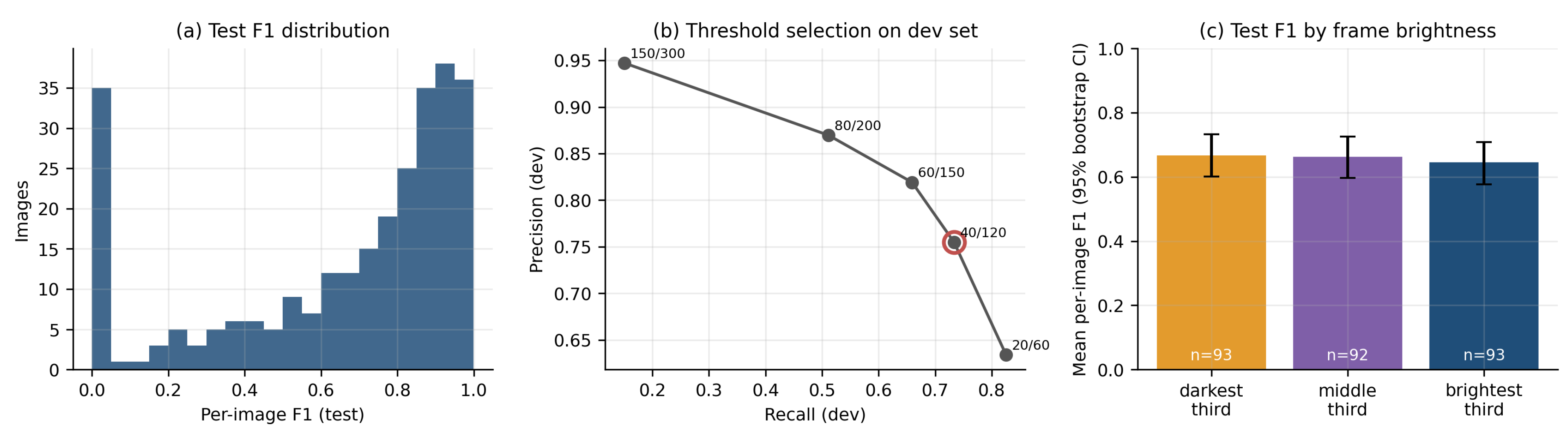
Results. On the development set, F1 peaks at thresholds 40/120 (0.695); the looser 20/60 (0.675) and tighter 60/150 (0.670) are close, but 150/300 collapses to 0.185 as recall falls to 0.15 (Figure 6b). On the test set (Table IV), precision is 0.734 [0.695, 0.770], recall 0.700 [0.661, 0.736] and F1 0.658 [0.620, 0.694], so H2a is supported. The per-image F1 distribution is bimodal (Figure 6a): the median frame is detected well (median precision 0.862, median recall 0.838), but 20 frames (7.2%) yield no detection and 14.0% have recall below 0.2. H2b is not supported: F1 is statistically indistinguishable across brightness terciles (Kruskal–Wallis p = 0.93). Visual inspection (Figure 5) attributes failures instead to worn or occluded markings, strong shadows, glare, and dense traffic that masks the markings. Global brightness is therefore a poor proxy for difficulty.
Table IV.
Classical Lane Detection on 278 Held-Out Frames (E2)
| Subset | n | Precision [95% CI] | Recall [95% CI] | F1 [95% CI] |
|---|---|---|---|---|
| All test frames | 278 | 0.734 [0.695, 0.770] | 0.700 [0.661, 0.736] | 0.658 [0.620, 0.694] |
| Darkest third (grey level 7–66) | 93 | — | — | 0.667 [0.601, 0.733] |
| Middle third (67–86) | 92 | — | — | 0.663 [0.597, 0.725] |
| Brightest third (87–151) | 93 | — | — | 0.645 [0.577, 0.708] |
Figure 5.
Test-set lane detections at high, median and low recall (E2). Top: detected segments (cyan), human labels (red) and ROI (yellow). Bottom: Canny edges inside the ROI.
Figure 5.
Test-set lane detections at high, median and low recall (E2). Top: detected segments (cyan), human labels (red) and ROI (yellow). Bottom: Canny edges inside the ROI.
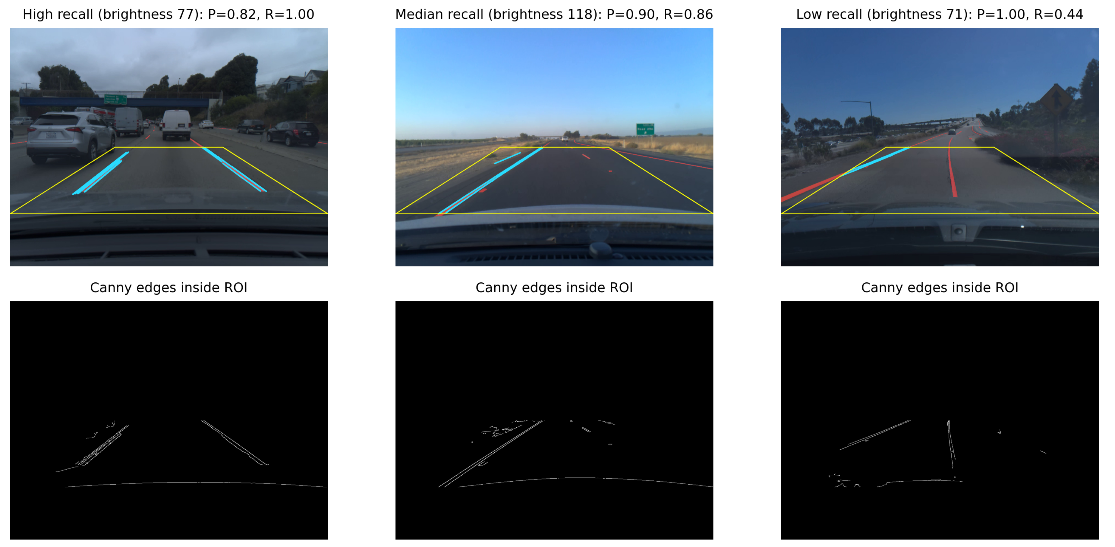
Figure 6.
Lane detection results (E2). (a) Per-image test F1. (b) Precision–recall trade-off of Canny thresholds on the development set; the selected setting is circled. (c) Test F1 by brightness tercile with 95% bootstrap CIs.
Figure 6.
Lane detection results (E2). (a) Per-image test F1. (b) Precision–recall trade-off of Canny thresholds on the development set; the selected setting is circled. (c) Test F1 by brightness tercile with 95% bootstrap CIs.
3). E3: Contribution of Context Features to Drivable-Area Segmentation
Objective and hypothesis. To isolate the contribution of spatial position, colour and local context to learned drivable-area segmentation, the mechanisms that deep networks exploit at scale [20,27]. H3: each added feature group significantly increases test IoU.
Setup. Frames are downsampled eightfold to 146 × 109 pixels, and the drivable label is road plus lane markings. Four nested feature sets are compared: position (normalised row, normalised column and horizontal offset from the image centre; 3 features), colour (BGR, HSV and Lab; 9 features), position + colour (12), and all features (26), which add 14 texture and context features: local grey-level mean and standard deviation in 3 × 3, 7 × 7 and 15 × 15 windows, Sobel gradient magnitude and its 9 × 9 average, and colour averaged over 9 × 9 and 25 × 25 windows. The classifier is scikit-learn’s HistGradientBoostingClassifier (200 iterations, learning rate 0.1, 63 leaf nodes) [87], trained on 250,000 pixels sampled from the 250 training frames. As a non-learned reference, the spatial-prior baseline labels a pixel drivable if more than 50% of training masks do. The pipeline is shown in Figure 4b.
| Algorithm 3 Feature-set ablation (E3) |
|
Results. Table V and Figure 7Figure 8 show the results. Seed variation is negligible (standard deviation of mean IoU ≤ 0.002 across seeds), so the CIs reflect frame-to-frame variability. Position alone reaches IoU 0.701, which equals the non-learned spatial prior (median paired difference ). Colour alone is much worse (0.521) and the most variable across frames (SD 0.227), because road appearance varies with lighting and surface. Combining the two adds 0.071 over position ( = 0.70), and texture and context add a further 0.022 ( = 0.68); both steps are significant after Holm correction (p < ), supporting H3. Remaining errors concentrate at road boundaries, at low light and where pavement resembles the road (Figure 8). The steadily diminishing but significant gains from wider context are consistent with the success of large-receptive-field CNN and Transformer models, which this small classical model does not attempt to match.
Table V.
Drivable-Area Segmentation on 150 Held-Out Frames (E3)
| Feature set | Features | Road IoU [95% CI] | Paired comparison | Median | p (Holm) | |
|---|---|---|---|---|---|---|
| Spatial prior (no learning) | — | 0.701 [0.680, 0.721] | — | — | — | — |
| Position | 3 | 0.701 [0.679, 0.721] | vs spatial prior | 0.017 | ||
| Colour | 9 | 0.521 [0.484, 0.556] | — | — | — | — |
| Position + colour | 12 | 0.773 [0.753, 0.793] | vs position; vs colour | +0.071; +0.209 | 0.70; 0.98 | ; |
| All (+ texture, context) | 26 | 0.803 [0.785, 0.821] | vs position + colour | +0.022 | 0.68 |
B. RQ2: State Estimation and Mapping
1). E5: GNSS–Odometry Fusion Under a GNSS Outage
Objective and hypothesis. To quantify the benefit of fusing complementary sensors and to compare linearisation strategies. H5a: fusion reduces RMSE relative to GNSS alone, especially during an outage. H5b: EKF and UKF perform equivalently for this mildly nonlinear model.
Setup. A vehicle follows a 120 s curved route at speeds varying between 12 and 28 m/s. Wheel-speed ( = 0.3 m/s) and yaw-rate ( = 0.02 rad/s, bias 0.01 rad/s) odometry arrive at 10 Hz. GNSS fixes ( = 3 m) arrive at 1 Hz, except during a 20 s outage (t = 50–70 s). Five estimators are compared: dead reckoning; GNSS only (holding the last fix); a linear constant-velocity Kalman filter (KF) using GNSS only; and an extended (EKF) and unscented (UKF) [39] Kalman filter that fuse odometry with GNSS. The fusion filters use the state x = [x, y, , and the unicycle motion model
with the standard KF prediction and update [9,38]:
where F is the Jacobian of f (EKF), or the unscented transform is used instead (UKF). Figure 9a shows the filter structure and the outage switch.
| Algorithm 4 Fusion experiment (E5) |
|
Results. Table VI and Figure 10 show the results. Dead reckoning diverges (420 m RMSE) because gyro bias integrates into heading error. GNSS alone is unbiased but noisy (11.2 m) and fails during the outage (265.5 m). Fusion reduces RMSE to 2.7 m with GNSS available and to 30.2 m during the outage. The EKF improves on GNSS alone in all 50 runs ( = , = 5.3 ×), supporting H5a. The EKF–UKF comparison illustrates the difference between statistical and practical significance. The overall RMSE difference is significant ( = 0.0011) because the 50 paired runs are highly correlated, but its median is only 7 mm, 0.06% of the error, and it reverses sign between the nominal (EKF better by 0.07 m) and outage periods. We therefore regard H5b as supported in practical terms.
Table VI.
Position RMSE in Metres Over 50 Monte Carlo Runs, Mean [95% CI] (E5)
| Estimator | Overall | GNSS available | 20 s outage | 95th percentile |
|---|---|---|---|---|
| Odometry only | 420.0 [410.3, 429.7] | 437.2 [427.2, 447.1] | 319.7 [311.1, 328.4] | 756.1 |
| GNSS only | 108.6 [108.3, 108.9] | 11.22 [11.15, 11.29] | 265.5 [264.8, 266.3] | 321.6 |
| Linear KF (GNSS only) | 119.2 [117.3, 121.1] | 4.80 [4.72, 4.88] | 292.5 [287.9, 297.2] | 337.2 |
| EKF (odometry + GNSS) | 12.57 [11.85, 13.29] | 2.71 [2.66, 2.77] | 30.24 [28.42, 32.05] | 34.2 |
| UKF (odometry + GNSS) | 12.56 [11.84, 13.29] | 2.78 [2.73, 2.83] | 30.18 [28.36, 32.00] | 34.2 |
2). E6: Effect of Pose Accuracy on Occupancy-Grid Mapping
Objective and hypothesis. To measure how pose error propagates into map quality. H6: landmark-corrected EKF poses yield significantly better maps than odometry.
Setup. A vehicle traverses a closed 656-pose route (0.1 s steps) in an 80 m × 60 m world with boundary walls and five rectangular obstacles, carrying a lidar (180 beams, 25 m range, = 3 cm). An occupancy grid (0.25 m cells) is updated every tenth pose in log-odds form [9,43]:
with log-odds clipped to , 4]. Three pose sources are compared: ground truth; odometry with a 2% scale error, a 0.004 rad/s yaw-rate bias and noise; and an EKF that corrects the same odometry with range-bearing observations ( = 0.3 m, ) of 12 known landmarks, modelled as
The procedure repeats trajectory noise, odometry, observations and mapping for 10 seeds. Map quality is the IoU of occupied cells against the true map, evaluated on cells observed with ground-truth poses. Figure 9b shows the loop. Script: exp06_localization_mapping.py.
Results. Table VII and Figure 11 show the results. Odometry drift (4.61 m RMSE, 10.1 m final error) destroys map structure (IoU 0.086) even though 95% of observed cells are still classified correctly, which shows why cell accuracy is a misleading map metric. The EKF reduces pose RMSE to 0.277 m and raises IoU to 0.502. It improves IoU in all ten seeds (Wilcoxon p = 0.002, = 1), supporting H6. The remaining gap to perfect poses (0.994) indicates that sub-cell pose accuracy is needed for crisp maps, which motivates joint pose-graph optimisation with loop closure [41,42].
Table VII.
Occupancy Mapping Over 10 Seeds, Mean [95% CI] (E6)
| Pose source | Pose RMSE (m) | Final pose error (m) | Cell accuracy | Occupied-cell IoU |
|---|---|---|---|---|
| Ground truth | 0 | 0 | 1.000 | 0.994 [0.993, 0.996] |
| Odometry | 4.61 [4.23, 4.98] | 10.11 [9.23, 10.99] | 0.951 [0.950, 0.952] | 0.086 [0.076, 0.096] |
| EKF with landmarks | 0.277 [0.269, 0.285] | 0.18 [0.11, 0.25] | 0.979 [0.977, 0.980] | 0.502 [0.473, 0.531] |
C. RQ2: Prediction, Planning and Decision-Making
1). E7: Physics-Based, Learned, Unimodal and Multimodal Trajectory Prediction
Objective and hypothesis. To determine whether learned and multimodal predictors improve on physics-based baselines, and why. H7a: the learned MLP has a lower ADE than constant velocity (CV). H7b: the multimodal predictor’s advantage comes from outputting several hypotheses rather than from a better model.
Setup. Trajectories are generated at 10 Hz for seven manoeuvres: keep lane, left and right turn, brake to stop, left and right lane change, and accelerate. Initial speed is uniform in 6–16 m/s, and acceleration ( = 0.15 ), yaw-rate noise ( = 0.01 rad/s) and position noise ( = 5 cm) are added. Manoeuvre onset is drawn uniformly between 0.5 s before and 0.8 s after the prediction time, so intent is sometimes invisible in the history. Each trajectory is normalised to the agent’s pose at the prediction time; models observe 2 s and predict 3 s. Table VIII lists the models; they are trained on 12,000 and tested on 3,000 trajectories per seed.
Table VIII.
Trajectory Predictors Compared in E7
| Model | Type | Outputs | Configuration |
|---|---|---|---|
| Constant velocity (CV) | Physics | 1 | Velocity from the last 0.5 s |
| CTRV | Physics | 1 | Speed and yaw rate from the last 1 s |
| MLP regressor | Learned | 1 | 2 × 256 ReLU layers, Adam, early stopping, standardised inputs and targets |
| k-NN top-1 | Learned (library) | 1 | Nearest training history (Euclidean, standardised) |
| k-NN library | Learned (library) | 6 | Futures of the six nearest histories; scored with |
Figure 12 shows how the history is normalised, which predictors produce single or multiple hypotheses, and which metrics apply to each.
Procedure. For seed s ∈ {7, …, 11}, a new dataset is generated, the MLP is trained with seed s, and all models are scored with Eq. (4). Metrics are averaged over test trajectories within a seed, and t CIs are computed over the five seeds. Paired Wilcoxon tests over the 3,000 trajectories of seed 7 compare MLP vs CV, k-NN-6 vs MLP and k-NN-1 vs MLP, with Holm correction. Script: exp07_trajectory_prediction.py.
Results. Table IX and Figure 13 show the results. The MLP has the lowest mean ADE among single-output models (2.49 m versus 2.78 m for CV, with non-overlapping CIs), but its per-trajectory median difference from CV is not significant ( = 0.72). It also has the highest miss rate (86.6%). Both observations follow from mean regression: under ambiguous intent, a squared-error model predicts the conditional mean, which reduces large errors on average but rarely lands within 2 m of any actual outcome (Figure 13c). H7a is therefore only partly supported. The multimodal library halves ADE and FDE (1.43 m and 3.56 m) and has the lowest miss rate (45.3%). Its single-hypothesis variant, however, is the worst model of all (ADE 3.56 m; worse than MLP with = 0.49, < ). This supports H7b: the benefit comes from covering several futures, not from a better predictor, which is why forecasting benchmarks and planners must consume trajectory distributions [45,46].
Table IX.
Trajectory Prediction Over a 3 s Horizon, Mean [95% CI] Over 5 Seeds (E7)
| Model | ADE (m) | FDE (m) | Miss rate (%) |
|---|---|---|---|
| Constant velocity | 2.782 [2.756, 2.807] | 7.60 [7.52, 7.67] | 68.9 [67.6, 70.3] |
| CTRV | 2.812 [2.792, 2.833] | 7.72 [7.66, 7.79] | 79.8 [78.7, 80.8] |
| MLP (single output) | 2.490 [2.458, 2.522] | 6.90 [6.79, 7.01] | 86.6 [84.0, 89.3] |
| k-NN top-1 | 3.563 [3.478, 3.647] | 9.74 [9.51, 9.98] | 82.4 [81.7, 83.1] |
| k-NN library, best of 6 | 1.428 [1.400, 1.455] | 3.56 [3.49, 3.63] | 45.3 [43.7, 46.9] |
2). E8: Heuristic Graph Search
Objective and hypothesis. To quantify the effect of heuristic admissibility and weighting in A* [51]. H8: the tight admissible octile heuristic expands significantly fewer nodes than Dijkstra’s algorithm [50] and the Euclidean heuristic without losing optimality, while inadmissible and weighted variants trade path cost for speed.
Setup and procedure. Fifty 200 × 200 grids are generated with seed 11, each with 45 random rectangular obstacles (sides 4–28 cells), and 49 of them admit a corner-to-corner path. Search is 8-connected with unit and step costs and no corner cutting. Five planners expand nodes in order of
with h = 0 (Dijkstra), Manhattan (inadmissible on 8-connected grids), Euclidean, octile ( = 1), and weighted octile ( = 2). Every planner solves every map; we record nodes expanded, runtime and excess cost relative to Dijkstra, and run Wilcoxon tests over maps with Holm correction. Script: exp08_path_planning.py. Figure 14 shows the search loop.
Results. Table X and Figure 15 show the results. The octile heuristic expands 3.84 times fewer nodes than Dijkstra (8,044 versus 30,884) and 32% fewer than Euclidean, and it returns optimal paths on all maps (≤ 1.1 ×, = ). This supports H8. The inadmissible Manhattan heuristic and weighted A* expand about 15 times fewer nodes than octile A*, at a mean cost increase of 1.9–2.0% and a worst case of 9.5%, far below the theoretical bound of 100% for = 2 but material for safety-relevant clearance decisions.
Table X.
Grid Planning Over 49 Solvable Maps, Mean [95% CI] (E8)
| Planner | Nodes expanded | Runtime (ms) | Excess cost (%) | Worst excess (%) |
|---|---|---|---|---|
| Dijkstra (h = 0) | 30,884 | 122.2 | 0 (optimal) | 0 |
| A*, Manhattan | 539 | 2.8 | 1.97 [1.25, 2.70] | 9.5 |
| A*, Euclidean | 11,853 | 84.5 | 0 (optimal) | 0 |
| A*, octile | 8,044 | 43.2 | 0 (optimal) | 0 |
| Weighted A*, octile, = 2 | 518 | 3.2 | 1.90 [1.21, 2.58] | 8.4 |
3). E9: Learned Anticipation Versus Rules for Lane-Change Decisions
Objective and hypothesis. To test whether a learned policy outperforms hand-written rules when both have identical information. H9: Q-learning [53] achieves a significantly lower crash rate than a rule with the same lookahead.
Setup. A three-lane highway is discretised into cells. Slower traffic approaches the ego vehicle by one cell per step, and each lane of a newly spawned row is occupied with probability 0.10 (never all three). Actions are keep lane, move left and move right. The reward is +1 per step, per lane change, for an invalid move and for a collision, which ends the episode; episodes last at most 200 steps. The state is the ego lane plus the occupancy of the three cells ahead in each lane (1,536 states). The tabular Q-learning update is
Four policies are compared: uniform random; a reactive rule that changes to a free adjacent lane when the next cell is blocked (one-cell lookahead); a gap-seeking rule that moves to the reachable lane with the longest free gap within three cells (the same information as the learned policy); and Q-learning. Figure 16 shows the training and evaluation loops.
| Algorithm 5 Training and evaluation of lane-change policies (E9) |
|
Results. Table XI and Figure 17 show the results. Q-learning crashes in 6.3% [5.5, 7.1] of test episodes, versus 59.8% for the gap-seeking rule; it is better in all ten seeds (p = 0.002, median difference percentage points), supporting H9. Extra lookahead alone does not help the rule: the gap-seeking and reactive rules do not differ (p = 0.28). The learned policy visits 834 of the 1,536 states and anticipates configurations that become unescapable two steps later, when two lanes close and the free lane is not adjacent. It moves pre-emptively, making 2.9 times as many lane changes as the rules. This behaviour would require comfort and traffic-law constraints before real deployment.
Table XI.
Lane-Change Policies on 500 Held-Out Episodes, Mean [95% CI] Over 10 Seeds (E9)
| Policy | Lookahead | Crash rate (%) | Steps survived | Lane changes per 100 steps |
|---|---|---|---|---|
| Random | — | 100.0 | 12.2 [11.9, 12.4] | 66.9 [66.3, 67.5] |
| Reactive rule | 1 cell | 60.4 [58.4, 62.3] | 133.0 [130.3, 135.7] | 9.34 [9.27, 9.42] |
| Gap-seeking rule | 3 cells | 59.8 [58.7, 60.9] | 133.8 [131.6, 136.0] | 9.38 [9.30, 9.46] |
| Q-learning | 3 cells | 6.3 [5.5, 7.1] | 193.5 [192.6, 194.4] | 26.8 [24.0, 29.7] |
D. RQ3: Motion Control
1). E10: Path-Tracking Controllers Under a Common Tuning Protocol
Objective and hypothesis. To compare geometric and optimisation-based lateral controllers fairly. H10a: model-based controllers (LQR, MPC) achieve the lowest tracking error at both speeds. H10b: MPC produces the smoothest steering.
Setup. The plant is a kinematic bicycle model [61] with wheelbase L = 2.7 m, a first-order steering actuator (time constant 0.1 s), a steering limit, a rate limit and pose-measurement noise ( = 3 cm, ), simulated at 20 Hz:
Pure Pursuit [59] steers toward a look-ahead point at distance = max(2, + 2), and Stanley [60] combines heading error with front-axle cross-track error e:
The LQR [62] and MPC [63] act on the linearised error dynamics with curvature and feed-forward = . LQR uses the discrete-time Riccati solution with Q = diag(1, 2) and input weight R:
MPC solves, at every step, a 20-step (1 s) horizon problem with CVXPY and OSQP [65,66]:
subject to the linearised dynamics of Eq. (18), ≤ and −≤.
The test reference (430 m) comprises a 3.5 m lane change and left and right curves (minimum radius 45 m). A separate validation reference (320 m) has a shorter lane change and curves in the opposite order with different radii. The first second of each run is excluded from the metrics. Figure 18 shows the closed loop and the outer tuning loop.
| Algorithm 6 Controller tuning and testing (E10) |
|
Results. Table XII reports the tuning results. The Pure Pursuit and LQR grids initially selected values at their edges, so both grids were extended until the optimum was interior; LQR with R = 1 diverged on the validation path. Table XIII and Figure 19 report the test results. No controller dominates, and H10a is not supported. At 8 m/s, Pure Pursuit is the most accurate (2.2 cm RMS) and Stanley the least (4.6 cm); at 15 m/s the ranking reverses, with Stanley best (1.9 cm) and LQR worst (6.4 cm). Stanley’s effective gain k/(1 + v) roughly doubles as speed halves, which makes it oscillatory at low speed after tuning at 12 m/s. H10b is supported: MPC has the lowest steering rate at both speeds (3.0 and ), is second most accurate at both speeds, and beats LQR in all ten seeds on both error ( cm) and smoothness (; = 0.008). The price of MPC is computation, 3.4 ms per step (99th percentile 4.5 ms) versus under 0.03 ms for the other controllers, although this is well within the 50 ms control period. Importantly, these rankings differ from those in a preliminary run of this experiment that used hand-picked gains, in which LQR appeared best. Unequal tuning is thus a first-order confounder in controller comparisons.
Table XII.
Validation Tuning of Controller Parameters at 12 m/s (E10)
| Controller | Tuned parameter | Grid | Selected | J at selection |
|---|---|---|---|---|
| Pure Pursuit | Look-ahead gain (s) | 0.1, 0.2, 0.3, 0.45, 0.6, 0.8 | 0.3 | 0.110 |
| Stanley | Cross-track gain k | 0.5, 1, 2, 3, 5 | 2.0 | 0.073 |
| LQR + feed-forward | Input weight R | 1 (diverged), 4, 16, 32, 64, 128, 256 | 32 | 0.116 |
| Linear MPC | Steering-rate weight S | 5, 20, 40, 80, 160 | 40 | 0.097 |
Table XIII.
Path Tracking on the 430 m Test Path, Mean [95% CI] Over 10 Noise Seeds (E10)
| Controller | RMS error 8 m/s (cm) | RMS error 15 m/s (cm) | Max error 15 m/s (cm) | RMS steering rate 8 / 15 m/s | Compute (ms) |
|---|---|---|---|---|---|
| Pure Pursuit | 2.2 [2.1, 2.2] | 5.8 [5.7, 5.9] | 12.2 | 6.59 / 3.67 | 0.01 |
| Stanley | 4.6 [4.5, 4.6] | 1.9 [1.9, 2.0] | 5.7 | 6.02 / 4.41 | 0.01 |
| LQR + feed-forward | 3.5 [3.5, 3.6] | 6.4 [6.3, 6.5] | 13.7 | 4.18 / 4.41 | 0.01 |
| Linear MPC (N = 20) | 2.8 [2.7, 2.8] | 5.6 [5.5, 5.7] | 12.4 | 3.00 / 3.46 | 3.4 |
E. RQ4: Field Evidence and Fleet Learning
1). E11: Statistical Re-Analysis of Public AV Safety Data
Objective and hypothesis. To verify the published safety comparison independently and to quantify the evidence it can support. H11a: rider-only crash rates are significantly below human benchmarks for every crash type. H11b: current exposure is insufficient to demonstrate a fatality-rate reduction.
Setup and procedure. For each of nine crash types with any reported injury, the hub provides the observed Waymo count k and the benchmark-expected count E, which is the human benchmark rate applied to Waymo’s mileage [6,17]. We computed the rate ratio k/E with the exact interval of Eq. (9), treating E as fixed, and aggregated over types. For exposure, a fleet with true rate (1 − that observes its expected count k after n miles demonstrates a lower rate than the human rate at 95% confidence when
We solve Eq. (20) for n numerically, for ∈ [0.2, 0.95] and three outcomes: fatalities ( = 1.19 per 100 million VMT [1]), serious-injury-or-worse crashes (0.23 IPMM) and any-injury-reported crashes (3.91 IPMM) [6]. Script: exp11_public_safety_data.py. Figure 20 traces the provenance of every quantity used.
Results. Through March 2026 the service logged 220.6 million RO miles (Figure 21a), and crash rates are below the benchmark in every city (Figure 21b). Across types, 142 crashes were observed against 834 expected, a ratio of 0.170 [0.143, 0.201] or an 83.0% reduction, consistent with the hub’s 81.9% headline within rounding. Every type’s upper CI limit is below 1 (Table XIV, Figure 21c), supporting H11a. The effect is heterogeneous. Intersection , single-vehicle and pedestrian crashes fall most, whereas front-to-rear and secondary crashes fall least; these categories often involve the AV being struck, which bounds what the AV’s own driving can prevent. For exposure (Table XV, Figure 22b), demonstrating an 80% fatality reduction requires about 388 million miles, and 252 million even with zero fatalities, both more than the current total. Current exposure is ample for injury outcomes (1.2 million miles for an 80% reduction), which supports H11b. California DMV reports (Figure 22a) show testing mileage of 4.5–9.1 million miles per year, two orders of magnitude short of fatality-level evidence.
Table XIV.
Any-Injury-Reported Crashes by Type: Observed Versus Benchmark-Expected (E11)
| Crash type | Observed k | Expected E | Ratio k/E [exact 95% CI] | Reduction (%) |
|---|---|---|---|---|
| Vehicle-to-vehicle intersection | 13 | 340 | 0.038 [0.020, 0.065] | 96.2 |
| Single vehicle | 2 | 60 | 0.033 [0.004, 0.120] | 96.7 |
| Pedestrian | 6 | 81 | 0.074 [0.027, 0.161] | 92.6 |
| Motorcycle | 6 | 38 | 0.158 [0.058, 0.344] | 84.2 |
| Cyclist | 9 | 56 | 0.161 [0.073, 0.305] | 83.9 |
| All others | 3 | 17 | 0.176 [0.036, 0.516] | 82.4 |
| Vehicle-to-vehicle lateral | 11 | 57 | 0.193 [0.096, 0.345] | 80.7 |
| Secondary crash | 19 | 46 | 0.413 [0.249, 0.645] | 58.7 |
| Vehicle-to-vehicle front-to-rear | 73 | 139 | 0.525 [0.412, 0.660] | 47.5 |
| All types | 142 | 834 | 0.170 [0.143, 0.201] | 83.0 |
Table XV.
Miles Needed to Demonstrate a Rate Reduction at 95% One-Sided Confidence (E11)
| Outcome | Human rate | = 50% | = 80% | Zero events observed |
|---|---|---|---|---|
| Fatality | 1.19 per 100 M VMT | 969 M | 388 M | 252 M |
| Serious injury or worse | 0.23 IPMM | 50.2 M | 20.1 M | — |
| Any injury reported | 3.91 IPMM | 2.95 M | 1.18 M | — |
2). E12: Federated Learning Under Non-IID Fleet Data
Objective and hypothesis. To measure how much of the benefit of pooling fleet data federated averaging (FedAvg) [83] recovers when vehicles see systematically different conditions. H12a: FedAvg outperforms isolated local training. H12b: more local epochs improve FedAvg under non-IID data within a fixed number of rounds.
Setup. The 250 training frames of E3 are divided among ten simulated vehicles, 25 frames each. In the non-IID split, frames are sorted by mean brightness, so client means range from 18 to 119 grey levels; an IID random split serves as a reference. Each client trains a per-pixel MLP (26 → 32 → 1, ReLU, 897 parameters) with SGD (learning rate 0.05, batch size 256) on 1,200 sampled pixels per frame, using the E3 features. The server aggregates client models holding samples:
Figure 23 shows the architecture.
| Algorithm 7 Federated learning experiment (E12) |
|
Results. Table XVI and Figure 24 show the results. Isolated training generalises poorly (IoU 0.616 [0.601, 0.631]), and the clients with the darkest and brightest data are worst (0.555 and 0.524). FedAvg with one local epoch reaches 0.716 and recovers 54.1% [50.8, 57.4] of the gap to centralised training (0.800), supporting H12a. Five local epochs reach 0.753 and recover 74.4% [72.6, 76.3], nearly matching FedAvg on IID data (77.1%), which supports H12b within the 40-round budget. The ordering holds in all five seeds; with n = 5, the smallest attainable two-sided Wilcoxon p-value is 0.0625, so this conclusion rests on the non-overlapping CIs rather than on p < 0.05. Communication cost is 35.9 kB per round for all ten clients.
Table XVI.
Federated Drivable-Area Segmentation After 40 Rounds, Mean [95% CI] Over 5 Seeds (E12)
| Regime | Raw data shared | Test IoU | Gap recovered (%) |
|---|---|---|---|
| Local-only (mean of 10 clients) | No | 0.616 [0.601, 0.631] | 0 (reference) |
| FedAvg, non-IID, E = 1 | No | 0.716 [0.708, 0.723] | 54.1 [50.8, 57.4] |
| FedAvg, non-IID, E = 5 | No | 0.753 [0.750, 0.756] | 74.4 [72.6, 76.3] |
| FedAvg, IID, E = 1 (reference) | No | 0.758 [0.751, 0.764] | 77.1 [75.0, 79.2] |
| Centralised (pooled) | Yes | 0.800 [0.799, 0.801] | 100 (reference) |
V. Discussion
Figure 25 maps each research question to its hypotheses, experiments and outcomes, and Table XVII lists the supporting evidence. We now answer the research questions and draw practical implications.
Table XVII.
Summary of Hypotheses and Outcomes
| Hypothesis | Outcome | Key evidence |
|---|---|---|
| H1: lane markings occupy under 1% of pixels | Supported | 0.588% [0.561, 0.613] |
| H2a: held-out lane F1 exceeds 0.6 | Supported | F1 = 0.658 [0.620, 0.694] |
| H2b: lane F1 decreases in darker frames | Not supported | Kruskal–Wallis p = 0.93 |
| H3: each feature group raises segmentation IoU | Supported | +0.071 and +0.022; < |
| H5a: fusion beats GNSS, especially in outages | Supported | 30.2 m vs 265.5 m; = 5.3 × |
| H5b: EKF and UKF are equivalent | Supported (practically) | Median = 7 mm, significant but negligible |
| H6: EKF poses improve maps over odometry | Supported | IoU 0.502 vs 0.086; 10/10 seeds |
| H7a: learned MLP beats constant velocity | Partly supported | Lower mean ADE; median n.s.; highest miss rate |
| H7b: multimodal gain comes from hypothesis count | Supported | k-NN-6 best; k-NN-1 worst |
| H8: octile A* is faster and still optimal | Supported | fewer nodes than Dijkstra; 0% excess |
| H9: Q-learning beats a rule with identical inputs | Supported | 6.3% vs 59.8% crashes; p = 0.002 |
| H10a: LQR and MPC are most accurate at both speeds | Not supported | Rankings reverse with speed |
| H10b: MPC produces the smoothest steering | Supported | Lowest steering rate at both speeds |
| H11a: rates below benchmark for all crash types | Supported | All 9 upper CI limits < 1 |
| H11b: exposure insufficient for fatality claims | Supported | 388 M miles needed vs 220.6 M driven |
| H12a: FedAvg beats local training | Supported | 0.716 vs 0.616; CIs disjoint |
| H12b: more local epochs help under non-IID data | Supported | 74.4% vs 54.1% of gap recovered |
RQ1: perception. Learned models gain from spatial context in a graded way. A position prior alone explains most drivable-area performance (0.701 IoU), appearance adds 0.07, and local context a further 0.02. Each step is statistically robust but smaller than the last. Thin structures are extremely under-represented (lane markings are 0.6% of pixels), so loss weighting and instance-level metrics matter. The classical lane detector is adequate on median frames but fails abruptly on a sizeable minority (7.2% no detection), and its failures are not explained by global brightness. Robustness evaluations should therefore stratify by the physical causes of failure, such as marking wear, occlusion and glare, rather than by simple image statistics.
RQ2: estimation, prediction and planning. Sensor fusion provides the largest effect in the study, an order-of-magnitude error reduction during outages, whereas the choice between EKF and UKF is immaterial for mildly nonlinear vehicle models. In prediction, the key variable is output representation rather than model capacity. A single-output regressor trained on ambiguous futures averages them, and a multimodal output with six hypotheses beats every single-output model even when built from the worst single-output component. In planning, tight admissible heuristics deliver speed without sacrificing optimality, while inadmissible shortcuts carry bounded but non-zero cost. In decision-making, learning discovered an anticipatory strategy that hand-written rules with the same inputs missed, but at the cost of 2.9 times more lane changes, a behaviour that reward design must regulate.
RQ3: control. The central finding is methodological. When each controller was tuned by the same validation procedure, accuracy rankings reversed between 8 and 15 m/s, and they differed from rankings obtained with hand-picked gains. The only consistent advantage was MPC’s smoothness, obtained at about 3.4 ms per step. Controller comparisons should therefore report their tuning protocol and evaluate across the operating envelope; gain scheduling of geometric controllers with speed would be a natural next step.
RQ4: fleet learning and field evidence. Federated learning recovered up to three quarters of the accuracy lost by isolated training without sharing images, and additional local computation partly compensated for heterogeneity. The public field data support a large and statistically robust reduction in injury crashes for one Level 4 service, strongest for intersection and pedestrian crashes. Yet even 220 million miles cannot demonstrate a fatality-rate reduction, which confirms the argument of [16] with current data. Safety cases for rare, severe outcomes must combine field data with simulation, scenario-based testing and standards such as ISO 21448 [80], ISO/PAS 8800 [81] and UL 4600 [82].
Relation to end-to-end and foundation models. The mechanisms isolated here are the same ones that modern end-to-end and vision-language driving models exploit implicitly: context aggregation (E3), multimodal output (E7), anticipation learned from reward or data (E9), and learning from distributed fleets (E12) [12,13,73]. Our results suggest that evaluating such models requires the same safeguards used here: held-out and validation-tuned protocols, multimodal metrics, closed-loop evaluation [15], and effect sizes with uncertainty.
VI. Threats to Validity
Internal validity. Implementations are our own and simplified, so implementation choices could affect rankings. We mitigated this by using identical inputs for all methods, validation-based tuning in E2 and E10, extending tuning grids whose optimum lay at an edge, and releasing code for inspection. Tuning in E10 covered one parameter per controller at one speed, and rankings may change with richer tuning or gain scheduling. The E10 error metric is measured at the rear axle for all controllers, whereas Stanley regulates the front axle, which may favour or penalise it in curves.
External validity. E5–E10 use simplified simulations (kinematic models, grid worlds, synthetic trajectories) that isolate mechanisms but omit real vehicle dynamics, sensor artefacts and interactive traffic. The magnitudes reported here should not be transferred to production systems. comma10k frames come from one camera type and fleet, mostly on U.S. highways. The perception models are deliberately small classical learners rather than deep networks, because no GPU was available, so absolute IoU values understate the state of the art. E11 concerns one operator in five cities with little snow.
Construct validity. IoU at 1/8 resolution, pixel-tolerance lane matching, displacement-based prediction metrics, and RMS error with a steering-rate penalty ( = 0.01) are proxies for driving quality. Different weights would change E10’s selected parameters. The E11 benchmarks cannot be perfectly matched on time of day, trip mix or reporting completeness, and our re-analysis ignores uncertainty in the benchmark itself.
Conclusion validity. We pre-specified comparisons within each experiment and applied Holm correction, but we did not correct across experiments. With many replicates, negligible differences become significant (E5), so we report effect sizes and CIs. With few seeds (E12, n = 5), exact tests cannot reach p < 0.05, and conclusions rest on CIs. The E6 and E9 tests use 10 seeds, which provides limited power for small effects.
VII. Conclusion and Future Work
This paper presented a reproducible, statistically grounded evaluation of classical and AI-based methods across the AV software stack, using public driving images, seeded simulations and public field safety data under one protocol. Of seventeen pre-stated hypotheses, thirteen were supported, one was supported only in practical terms, one partly, and two were not supported. Three findings are especially relevant to practitioners. The advantage of multimodal predictors lies in their output representation. Controller rankings depend on tuning protocol and speed. Finally, current field exposure supports strong injury-reduction claims but not fatality-reduction claims.
Limitations. These findings should be read within the scope of the study. Six of the twelve experiments (E5–E10) use simplified, seeded simulations with kinematic vehicle models, grid worlds and synthetic trajectories. These isolate how the methods behave, but they do not capture real vehicle dynamics, sensor artefacts or interactive traffic, so the reported magnitudes should not be transferred to production systems. The learned perception models (E3, E12) are deliberately small classical learners trained on 250 frames from a single camera type, and the lane detector (E2) is a classical pipeline; no GPU-based deep networks were used. Absolute IoU and F1 values therefore understate the state of the art; the relative effects of context and multimodality are the intended contribution. Controller tuning covered one parameter per controller at a single validation speed (12 m/s), and other tuning budgets or gain scheduling could change the rankings. The field safety analysis concerns one operator in five cities, treats the published benchmarks as exact, and cannot address fatality outcomes with current exposure. In addition, large end-to-end and vision-language driving models were not evaluated directly. The protocol is designed to extend to them, but whether our conclusions hold at that scale remains an open question. Section VI discusses these threats in more detail.
Future work will replace the classical perception learners with deep networks on GPU hardware, evaluate on large multimodal datasets such as nuScenes [35] and the Waymo Open Motion Dataset [46], move planning and control experiments into closed-loop simulation such as CARLA [88] with interactive agents, and extend the protocol to end-to-end and vision-language driving models.
Supplementary Materials
The following supporting information can be downloaded at the website of this paper posted on Preprints.org.
Author Contributions
A. W.: conceptualisation, methodology, software, writing—original draft; S. G.: supervision, validation, writing—review and editing.
Data Availability Statement
Code, transcribed public data, per-replicate raw results and all figures are provided in the accompanying archive (av_ai_research_code.zip) [repository URL/DOI to be inserted]. comma10k is available at https://github.com/commaai/comma10k (MIT licence); the seeded sample is recorded in data/comma10k/sample_list.txt. Waymo Safety Impact Data Hub tables (data through March 2026) and California DMV totals were transcribed on 16 September 2026; source URLs are listed in data/public/SOURCES.md.
Conflicts of Interest
The authors declare no conflicts of interest.
Appendix A Verification of Worked Examples and Corrections to Version 1
Experiment E4 (exp04_verify_equations.py) numerically verifies the textbook examples that version 1 of this preprint [89] presented incorrectly.
Convolution. For input x = [[1, 2, 3], [4, 5, 6], [7, 8, 9]] and kernel w = [[1, 0], [0, , the cross-correlation computed by deep-learning libraries, y[i, j] = x[i + m, j + , n], gives , , , . True convolution flips the kernel and gives [[4, 4], [4, 4]]. Version 1 labelled the former as convolution.
Recurrent update. For = + + ), with = [0.5, , = [1.0, 0.5], = [[0.2, 0.4], [0.3, 0.1]], = [[0.5, 0.6], [0.7, 0.8]] and = [0.1, 0.2], the terms are = , 0.12] (version 1 reported [0.1, 0.12]), = [0.80, 1.10], and = tanh([0.88, 1.42]) = [0.706, 0.890] (version 1 reported [0.76, 0.89]).
Other corrections.
- The range-bearing model now includes the square root and uses atan2 (Eq. 13).
- The occupancy update uses the log-odds form (Eq. 12).
- The LQR cost’s control term is .
- The previously missing A* and Q-learning equations are Eqs. (14) and (15).
- Template text and unverifiable references were removed.
References
- National Highway Traffic Safety Administration. "Overview of motor vehicle traffic crashes in 2024," U.S. Dept. Transp., Washington, DC, USA, Traffic Safety Facts Research Note, Apr. 2026.
- Pomerleau, D. A. ALVINN: An autonomous land vehicle in a neural network. Proc. Adv. Neural Inf. Process. Syst. (NIPS), 1989; pp. 305–313. [Google Scholar]
- Thrun, S.; et al. Stanley: The robot that won the DARPA Grand Challenge. J. Field Robot. 2006, vol. 23(no. 9), 661–692. [Google Scholar] [CrossRef]
- Urmson, C.; et al. Autonomous driving in urban environments: Boss and the Urban Challenge. J. Field Robot. 2008, vol. 25(no. 8), 425–466. [Google Scholar] [CrossRef]
- SAE Standard J3016202104; Taxonomy and Definitions for Terms Related to Driving Automation Systems for On-Road Motor Vehicles. SAE International, 2021.
- Waymo LLC. Waymo safety impact data hub (data through March 2026). Available online: https://waymo.com/safety/impact/ (accessed on 16 September 2026).
- Grigorescu, S.; Trasnea, B.; Cocias, T.; Macesanu, G. A survey of deep learning techniques for autonomous driving. J. Field Robot. 2020, vol. 37(no. 3), 362–386. [Google Scholar] [CrossRef]
- Badue, C.; et al. Self-driving cars: A survey. Expert Syst. Appl. 2021, vol. 165, Art. no. 113816. [Google Scholar] [CrossRef]
- Thrun, S.; Burgard, W.; Fox, D. Probabilistic Robotics; MIT Press: Cambridge, MA, USA, 2005. [Google Scholar]
- Paden, B.; Čáp, M.; Yong, S. Z.; Yershov, D.; Frazzoli, E. A survey of motion planning and control techniques for self-driving urban vehicles. IEEE Trans. Intell. Veh. 2016, vol. 1(no. 1), 33–55. [Google Scholar] [CrossRef]
- Schwarting, W.; Alonso-Mora, J.; Rus, D. Planning and decision-making for autonomous vehicles. Annu. Rev. Control Robot. Auton. Syst. 2018, vol. 1, 187–210. [Google Scholar] [CrossRef]
- Hu, Y.; et al. Planning-oriented autonomous driving. Proc. IEEE/CVF Conf. Comput. Vis. Pattern Recognit. (CVPR), 2023; pp. 17853–17862. [Google Scholar]
- Chen, L.; Wu, P.; Chitta, K.; Jaeger, B.; Geiger, A.; Li, H. End-to-end autonomous driving: Challenges and frontiers. IEEE Trans. Pattern Anal. Mach. Intell. 2024, vol. 46(no. 12), 10164–10183. [Google Scholar] [CrossRef] [PubMed]
- Yurtsever, E.; Lambert, J.; Carballo, A.; Takeda, K. A survey of autonomous driving: Common practices and emerging technologies. IEEE Access 2020, vol. 8, 58443–58469. [Google Scholar] [CrossRef]
- Li, Z.; et al. Is ego status all you need for open-loop end-to-end autonomous driving? Proc. IEEE/CVF Conf. Comput. Vis. Pattern Recognit. (CVPR), 2024. [Google Scholar]
- Kalra, N.; Paddock, S. M. Driving to safety: How many miles of driving would it take to demonstrate autonomous vehicle reliability? Transp. Res. A Policy Pract. 2016, vol. 94, 182–193. [Google Scholar] [CrossRef]
- Kusano, K. D.; et al. Comparison of Waymo rider-only crash rates by crash type to human benchmarks at 56.7 million miles. Traffic Inj. Prev. 2025, vol. 26 suppl. 1, S8–S20. [Google Scholar] [CrossRef] [PubMed]
- Kato, S.; et al. Autoware on board: Enabling autonomous vehicles with embedded systems. Proc. ACM/IEEE Int. Conf. Cyber-Phys. Syst. (ICCPS), 2018; pp. 287–296. [Google Scholar]
- González, D.; Pérez, J.; Milanés, V.; Nashashibi, F. A review of motion planning techniques for automated vehicles. IEEE Trans. Intell. Transp. Syst. 2016, vol. 17(no. 4), 1135–1145. [Google Scholar] [CrossRef]
- Krizhevsky, A.; Sutskever, I.; Hinton, G. E. ImageNet classification with deep convolutional neural networks. Proc. Adv. Neural Inf. Process. Syst. (NIPS), 2012; pp. 1097–1105. [Google Scholar]
- Goodfellow, I.; Bengio, Y. A. Courville, Deep Learning; MIT Press: Cambridge, MA, USA, 2016. [Google Scholar]
- Ren, S.; He, K.; Girshick, R.; Sun, J. Faster R-CNN: Towards real-time object detection with region proposal networks. Proc. Adv. Neural Inf. Process. Syst. (NIPS), 2015; pp. 91–99. [Google Scholar]
- Redmon, J.; Divvala, S.; Girshick, R.; Farhadi, A. You only look once: Unified, real-time object detection. Proc. IEEE Conf. Comput. Vis. Pattern Recognit. (CVPR), 2016; pp. 779–788. [Google Scholar]
- Carion, N.; Massa, F.; Synnaeve, G.; Usunier, N.; Kirillov, A.; Zagoruyko, S. End-to-end object detection with transformers. Proc. Eur. Conf. Comput. Vis. (ECCV) 2020, 213–229. [Google Scholar] [CrossRef]
- Lang, A. H.; Vora, S.; Caesar, H.; Zhou, L.; Yang, J.; Beijbom, O. PointPillars: Fast encoders for object detection from point clouds. Proc. IEEE/CVF Conf. Comput. Vis. Pattern Recognit. (CVPR), 2019; pp. 12697–12705. [Google Scholar]
- Philion, J.; Fidler, S. Lift, splat, shoot: Encoding images from arbitrary camera rigs by implicitly unprojecting to 3D. Proc. Eur. Conf. Comput. Vis. (ECCV) 2020, 194–210. [Google Scholar] [CrossRef]
- Li, Z.; et al. BEVFormer: Learning bird’s-eye-view representation from multi-camera images via spatiotemporal transformers. Proc. Eur. Conf. Comput. Vis. (ECCV) 2022, 1–18. [Google Scholar] [CrossRef]
- Liu, Z.; et al. BEVFusion: Multi-task multi-sensor fusion with unified bird’s-eye view representation. Proc. IEEE Int. Conf. Robot. Autom. (ICRA), 2023; pp. 2774–2781. [Google Scholar]
- Cordts, M.; et al. The Cityscapes dataset for semantic urban scene understanding. Proc. IEEE Conf. Comput. Vis. Pattern Recognit. (CVPR), 2016; pp. 3213–3223. [Google Scholar]
- Yu, F.; et al. BDD100K: A diverse driving dataset for heterogeneous multitask learning. Proc. IEEE/CVF Conf. Comput. Vis. Pattern Recognit. (CVPR), 2020; pp. 2636–2645. [Google Scholar]
- Canny, J. A computational approach to edge detection. IEEE Trans. Pattern Anal. Mach. Intell. 1986, vol. PAMI-8(no. 6), 679–698. [Google Scholar] [CrossRef]
- Duda, R. O.; Hart, P. E. Use of the Hough transformation to detect lines and curves in pictures. Commun. ACM 1972, vol. 15(no. 1), 11–15. [Google Scholar] [CrossRef]
- Bradski, G. The OpenCV library. Dr. Dobb’s J. Softw. Tools 2000, vol. 25(no. 11), 120–125. [Google Scholar]
- Geiger, A.; Lenz, P.; Urtasun, R. Are we ready for autonomous driving? The KITTI vision benchmark suite. Proc. IEEE Conf. Comput. Vis. Pattern Recognit. (CVPR), 2012; pp. 3354–3361. [Google Scholar]
- Caesar, H.; et al. nuScenes: A multimodal dataset for autonomous driving. Proc. IEEE/CVF Conf. Comput. Vis. Pattern Recognit. (CVPR), 2020; pp. 11621–11631. [Google Scholar]
- Sun, P.; et al. Scalability in perception for autonomous driving: Waymo Open Dataset. Proc. IEEE/CVF Conf. Comput. Vis. Pattern Recognit. (CVPR), 2020; pp. 2446–2454. [Google Scholar]
- comma.ai. comma10k: Crowd-sourced semantic segmentation dataset of driving images," GitHub repository (MIT licence). Available online: https://github.com/commaai/comma10k (accessed on 16 September 2026).
- Kalman, R. E. A new approach to linear filtering and prediction problems. J. Basic Eng. 1960, vol. 82(no. 1), 35–45. [Google Scholar] [CrossRef]
- Julier, S. J.; Uhlmann, J. K. Unscented filtering and nonlinear estimation. Proc. IEEE 2004, vol. 92(no. 3), 401–422. [Google Scholar] [CrossRef]
- Durrant-Whyte, H.; Bailey, T. Simultaneous localization and mapping: Part I. IEEE Robot. Autom. Mag. 2006, vol. 13(no. 2), 99–110. [Google Scholar] [CrossRef]
- Mur-Artal, R.; Tardós, J. D. ORB-SLAM2: An open-source SLAM system for monocular, stereo, and RGB-D cameras. IEEE Trans. Robot. 2017, vol. 33(no. 5), 1255–1262. [Google Scholar] [CrossRef]
- Lowry, S.; et al. Visual place recognition: A survey. IEEE Trans. Robot. 2016, vol. 32(no. 1), 1–19. [Google Scholar] [CrossRef]
- Elfes, A. Using occupancy grids for mobile robot perception and navigation. Computer 1989, vol. 22(no. 6), 46–57. [Google Scholar] [CrossRef]
- Gao, J.; et al. VectorNet: Encoding HD maps and agent dynamics from vectorized representation. Proc. IEEE/CVF Conf. Comput. Vis. Pattern Recognit. (CVPR), 2020; pp. 11525–11533. [Google Scholar]
- Shi, S.; Jiang, L.; Dai, D.; Schiele, B. Motion transformer with global intention localization and local movement refinement. Proc. Adv. Neural Inf. Process. Syst. (NeurIPS), 2022; pp. 6531–6543. [Google Scholar]
- Ettinger, S.; et al. Large scale interactive motion forecasting for autonomous driving: The Waymo Open Motion Dataset. Proc. IEEE/CVF Int. Conf. Comput. Vis. (ICCV), 2021; pp. 9710–9719. [Google Scholar]
- Wilson, B.; et al. Argoverse 2: Next generation datasets for self-driving perception and forecasting. Proc. NeurIPS Datasets Benchmarks Track, 2021. [Google Scholar]
- Hochreiter, S.; Schmidhuber, J. Long short-term memory. Neural Comput. 1997, vol. 9(no. 8), 1735–1780. [Google Scholar] [CrossRef] [PubMed]
- Vaswani, A.; et al. Attention is all you need. Proc. Adv. Neural Inf. Process. Syst. (NIPS), 2017; pp. 5998–6008. [Google Scholar]
- Dijkstra, E. W. A note on two problems in connexion with graphs. Numer. Math. 1959, vol. 1, 269–271. [Google Scholar] [CrossRef]
- Hart, P. E.; Nilsson, N. J.; Raphael, B. A formal basis for the heuristic determination of minimum cost paths. IEEE Trans. Syst. Sci. Cybern. 1968, vol. 4(no. 2), 100–107. [Google Scholar] [CrossRef]
- Dolgov, D.; Thrun, S.; Montemerlo, M.; Diebel, J. Path planning for autonomous vehicles in unknown semi-structured environments. Int. J. Robot. Res. 2010, vol. 29(no. 5), 485–501. [Google Scholar] [CrossRef]
- Watkins, C. J. C. H.; Dayan, P. Q-learning. Mach. Learn. 1992, vol. 8(no. 3–4), 279–292. [Google Scholar] [CrossRef]
- Mnih, V.; et al. Human-level control through deep reinforcement learning. Nature 2015, vol. 518(no. 7540), 529–533. [Google Scholar] [CrossRef] [PubMed]
- Sutton, R. S.; Barto, A. G. Reinforcement Learning: An Introduction, 2nd ed.; MIT Press: Cambridge, MA, USA, 2018. [Google Scholar]
- Kiran, B. R.; et al. Deep reinforcement learning for autonomous driving: A survey. IEEE Trans. Intell. Transp. Syst. 2022, vol. 23(no. 6), 4909–4926. [Google Scholar] [CrossRef]
- Ross, S.; Gordon, G.; Bagnell, D. A reduction of imitation learning and structured prediction to no-regret online learning. Proc. Int. Conf. Artif. Intell. Stat. (AISTATS) 2011, 627–635. [Google Scholar]
- Bansal, M.; Krizhevsky, A.; Ogale, A. ChauffeurNet: Learning to drive by imitating the best and synthesizing the worst. Proc. Robot. Sci. Syst. (RSS) 2019. [Google Scholar] [CrossRef]
- Coulter, R. C. Implementation of the pure pursuit path tracking algorithm; Robotics Inst., Carnegie Mellon Univ.: Pittsburgh, PA, USA, Tech. Rep. CMU-RI-TR-92-01; Tech. Rep. CMU-RI-TR-92-01, 1992. [Google Scholar]
- Hoffmann, G. M.; Tomlin, C. J.; Montemerlo, M.; Thrun, S. Autonomous automobile trajectory tracking for off-road driving: Controller design, experimental validation and racing. Proc. Amer. Control Conf. (ACC), 2007; pp. 2296–2301. [Google Scholar]
- Rajamani, R. Vehicle Dynamics and Control, 2nd ed.; Springer: New York, NY, USA, 2012. [Google Scholar]
- Anderson, B. D. O.; Moore, J. B. Optimal Control: Linear Quadratic Methods; Prentice-Hall: Englewood Cliffs, NJ, USA, 1990. [Google Scholar]
- Mayne, D. Q.; Rawlings, J. B.; Rao, C. V.; Scokaert, P. O. M. Constrained model predictive control: Stability and optimality. Automatica 2000, vol. 36(no. 6), 789–814. [Google Scholar] [CrossRef]
- Qin, S. J.; Badgwell, T. A. A survey of industrial model predictive control technology. Control Eng. Pract. 2003, vol. 11(no. 7), 733–764. [Google Scholar] [CrossRef]
- Diamond, S.; Boyd, S. CVXPY: A Python-embedded modeling language for convex optimization. J. Mach. Learn. Res. 2016, vol. 17(no. 83), 1–5. [Google Scholar]
- Stellato, B.; Banjac, G.; Goulart, P.; Bemporad, A.; Boyd, S. OSQP: An operator splitting solver for quadratic programs. Math. Program. Comput. 2020, vol. 12(no. 4), 637–672. [Google Scholar] [CrossRef]
- Bojarski, M.; et al. End to end learning for self-driving cars. arXiv 2016, arXiv:1604.07316. [Google Scholar]
- Chitta, K.; Prakash, A.; Jaeger, B.; Yu, Z.; Renz, K.; Geiger, A. TransFuser: Imitation with transformer-based sensor fusion for autonomous driving. IEEE Trans. Pattern Anal. Mach. Intell. 2023, vol. 45(no. 11), 12878–12895. [Google Scholar] [CrossRef] [PubMed]
- Jiang, B.; et al. VAD: Vectorized scene representation for efficient autonomous driving. Proc. IEEE/CVF Int. Conf. Comput. Vis. (ICCV), 2023; pp. 8340–8350. [Google Scholar]
- Hu, A.; et al. GAIA-1: A generative world model for autonomous driving. arXiv 2023, arXiv:2309.17080. [Google Scholar]
- Kerbl, B.; Kopanas, G.; Leimkühler, T.; Drettakis, G. 3D Gaussian splatting for real-time radiance field rendering. ACM Trans. Graph. 2023, vol. 42(no. 4), Art. no. 139. [Google Scholar] [CrossRef]
- Tian, X.; et al. DriveVLM: The convergence of autonomous driving and large vision-language models. arXiv 2024, arXiv:2402.12289. [Google Scholar]
- Hwang, J.-J.; et al. EMMA: End-to-end multimodal model for autonomous driving. arXiv 2024, arXiv:2410.23262. [Google Scholar]
- National Highway Traffic Safety Administration. Third amended standing general order 2021-01: Incident reporting requirements for ADS and level 2 ADAS; U.S. Dept. Transp.: Washington, DC, USA, Apr 2025. [Google Scholar]
- Scanlon, J. M.; et al. Benchmarks for retrospective automated driving system crash rate analysis using police-reported crash data. Traffic Inj. Prev. 2024, vol. 25 suppl. 1, S51–S65. [Google Scholar] [CrossRef] [PubMed]
- Kusano, K. D.; et al. Comparison of Waymo rider-only crash data to human benchmarks at 7.1 million miles. Traffic Inj. Prev. 2024, vol. 25 suppl. 1, S66–S77. [Google Scholar] [CrossRef] [PubMed]
- California Department of Motor Vehicles. Autonomous vehicle disengagement reports and news releases. Available online: https://www.dmv.ca.gov/portal/vehicle-industry-services/autonomous-vehicles/ (accessed on 16 September 2026).
- Garwood, F. Fiducial limits for the Poisson distribution. Biometrika 1936, vol. 28(no. 3–4), 437–442. [Google Scholar] [CrossRef]
- ISO Standard 26262:2018; Road Vehicles—Functional Safety. 2018.
- ISO Standard 21448:2022; Road Vehicles—Safety of the Intended Functionality. 2022.
- ISO/PAS 8800:2024, 2024; Road Vehicles—Safety and Artificial Intelligence.
- Standard for Safety for the Evaluation of Autonomous Products, ANSI/UL Standard 4600, 3rd ed., 2023.
- McMahan, B.; Moore, E.; Ramage, D.; Hampson, S.; Agüera y Arcas, B. Communication-efficient learning of deep networks from decentralized data. Proc. Int. Conf. Artif. Intell. Stat. (AISTATS) 2017, 1273–1282. [Google Scholar]
- Kendall, A.; Gal, Y. What uncertainties do we need in Bayesian deep learning for computer vision? Proc. Adv. Neural Inf. Process. Syst. (NIPS), 2017; pp. 5574–5584. [Google Scholar]
- Selvaraju, R. R.; Cogswell, M.; Das, A.; Vedantam, R.; Parikh, D.; Batra, D. Grad-CAM: Visual explanations from deep networks via gradient-based localization. Proc. IEEE Int. Conf. Comput. Vis. (ICCV), 2017; pp. 618–626. [Google Scholar]
- Eykholt, K.; et al. Robust physical-world attacks on deep learning visual classification. Proc. IEEE/CVF Conf. Comput. Vis. Pattern Recognit. (CVPR), 2018; pp. 1625–1634. [Google Scholar]
- Pedregosa, F.; et al. Scikit-learn: Machine learning in Python. J. Mach. Learn. Res. 2011, vol. 12, 2825–2830. [Google Scholar]
- Dosovitskiy, A.; Ros, G.; Codevilla, F.; López, A.; Koltun, V. CARLA: An open urban driving simulator. Proc. Conf. Robot Learn. (CoRL), 2017; pp. 1–16. [Google Scholar]
- Waghmare, A. A.; Ganesan, S.; Chen, J. Role of artificial intelligence in autonomous vehicles. Preprints 2024, version 1. [Google Scholar] [CrossRef]
Figure 1.
System architecture of the autonomous vehicle stack used in this study. Parallelograms are data, rounded boxes are processing modules and labelled arrows are signals; dark tags mark the experiments that evaluate each module, and red labels mark research questions. Fleet learning (E12) and field safety evidence (E11) operate across vehicles. The same notation is used in all block diagrams.
Figure 1.
System architecture of the autonomous vehicle stack used in this study. Parallelograms are data, rounded boxes are processing modules and labelled arrows are signals; dark tags mark the experiments that evaluate each module, and red labels mark research questions. Fleet learning (E12) and field safety evidence (E11) operate across vehicles. The same notation is used in all block diagrams.
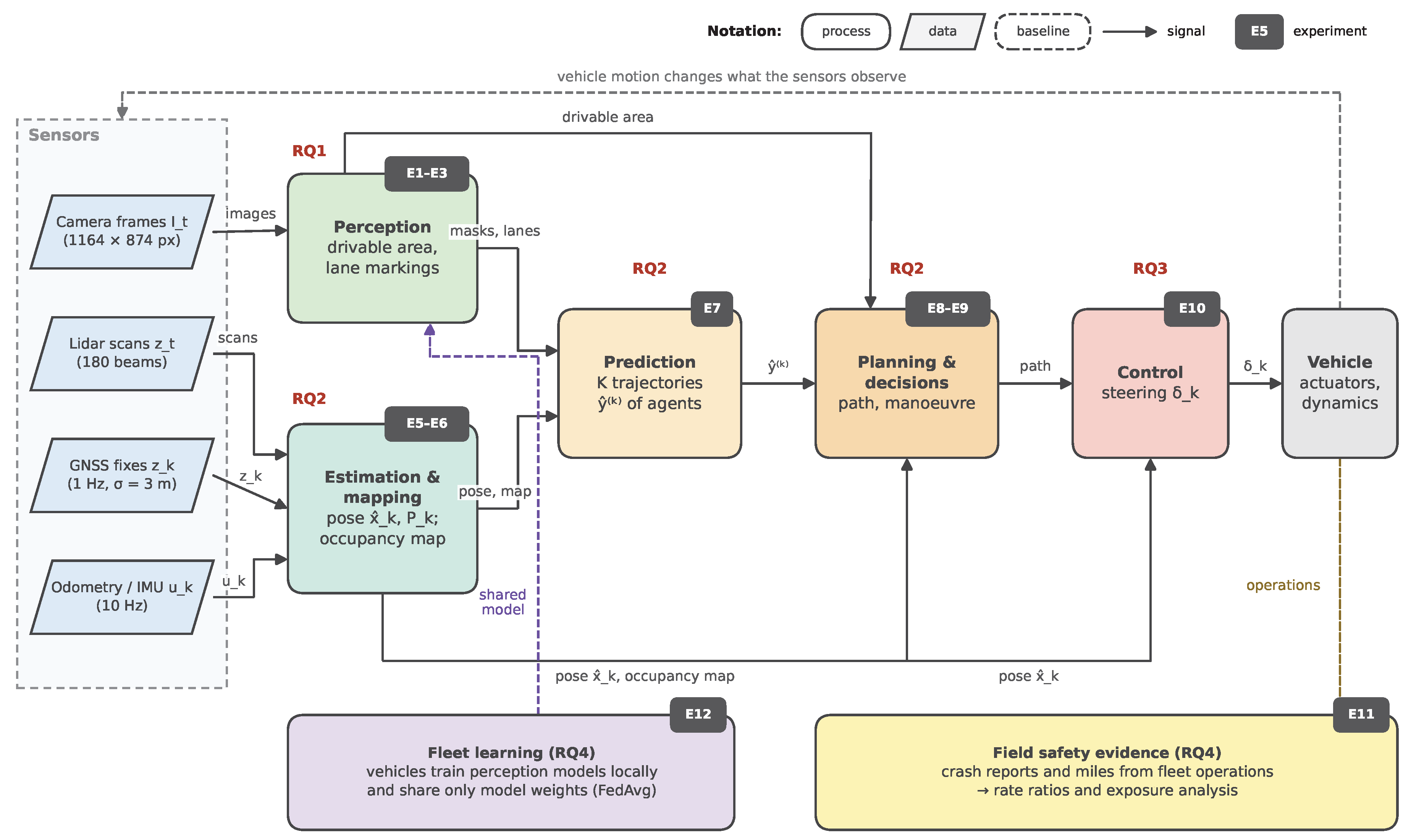
Figure 2.
Evaluation pipeline shared by all experiments. Splits and seeds are fixed first; parameters are selected on development or validation data only, and the frozen configuration is run once on held-out test data. The dashed red line marks the separation between tuning and testing.
Figure 2.
Evaluation pipeline shared by all experiments. Splits and seeds are fixed first; parameters are selected on development or validation data only, and the frozen configuration is run once on held-out test data. The dashed red line marks the separation between tuning and testing.

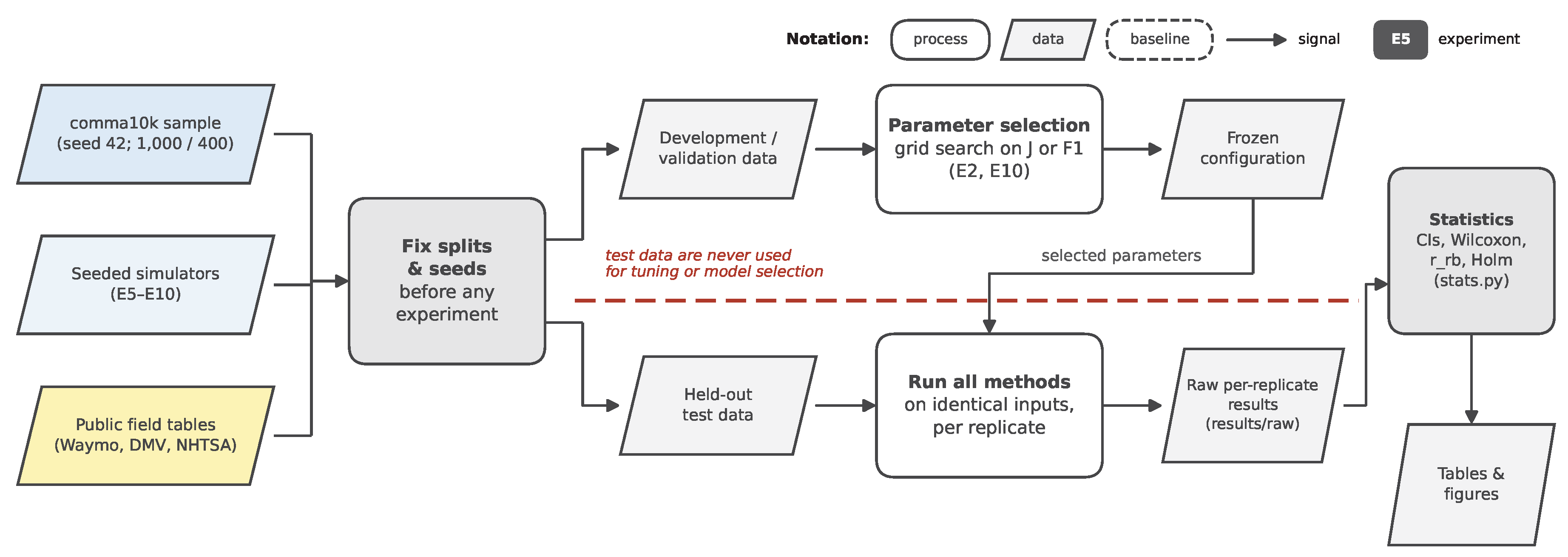
Figure 3.
Class statistics of 1,000 comma10k masks (E1). (a) Mean pixel share with 95% bootstrap CI. (b) Per-image distribution (log scale). (c) Empirical probability that a pixel is drivable.
Figure 3.
Class statistics of 1,000 comma10k masks (E1). (a) Mean pixel share with 95% bootstrap CI. (b) Per-image distribution (log scale). (c) Empirical probability that a pixel is drivable.
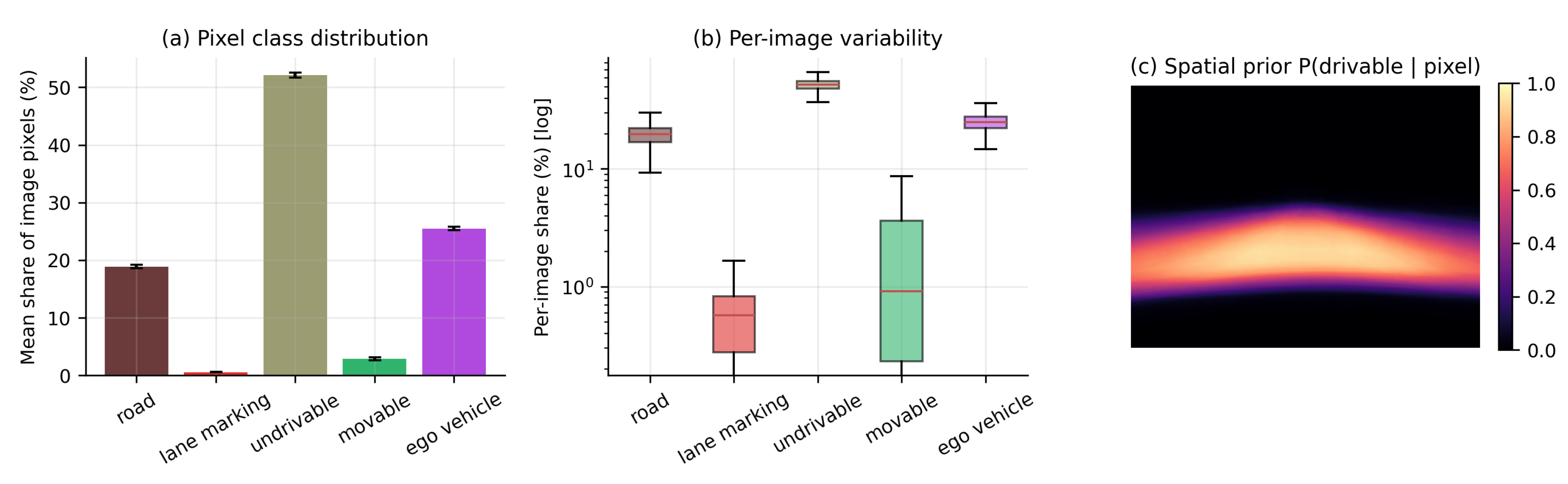
Figure 4.
Perception pipelines. (a) Classical lane detector of E2, with thresholds selected on the development set. (b) Learned drivable-area segmentation of E3: three feature branches with switches for the ablation, a gradient-boosted classifier, and the non-learned spatial-prior baseline.
Figure 4.
Perception pipelines. (a) Classical lane detector of E2, with thresholds selected on the development set. (b) Learned drivable-area segmentation of E3: three feature branches with switches for the ablation, a gradient-boosted classifier, and the non-learned spatial-prior baseline.
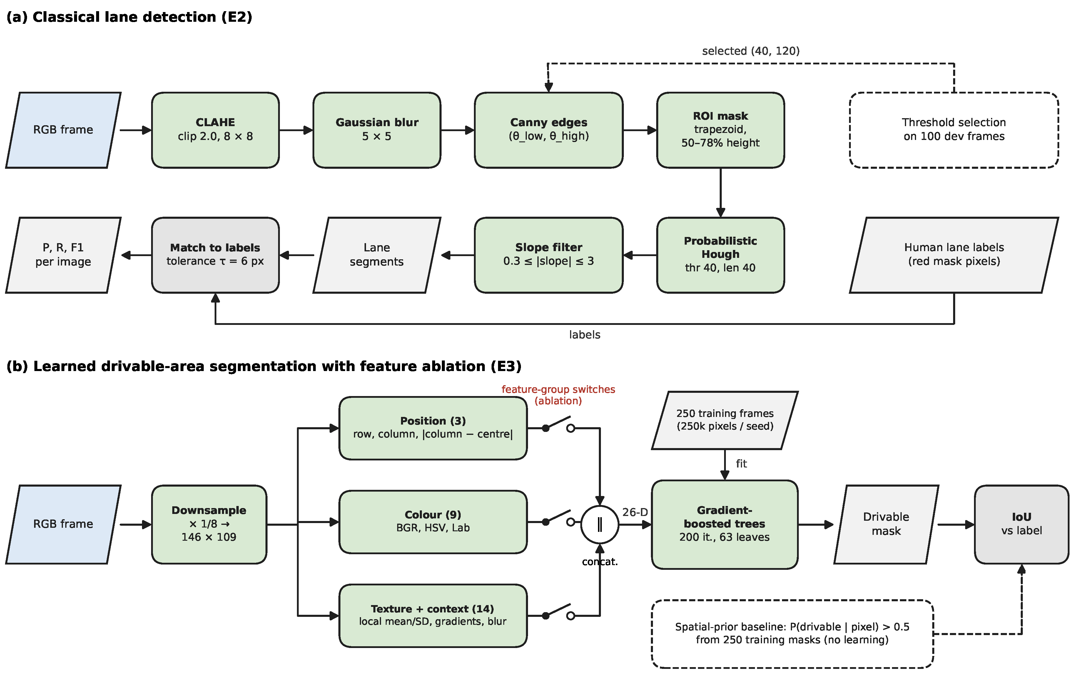
Figure 7.
Test IoU by feature set with 95% bootstrap CIs (E3). The dashed line marks the non-learned spatial-prior baseline.
Figure 7.
Test IoU by feature set with 95% bootstrap CIs (E3). The dashed line marks the non-learned spatial-prior baseline.
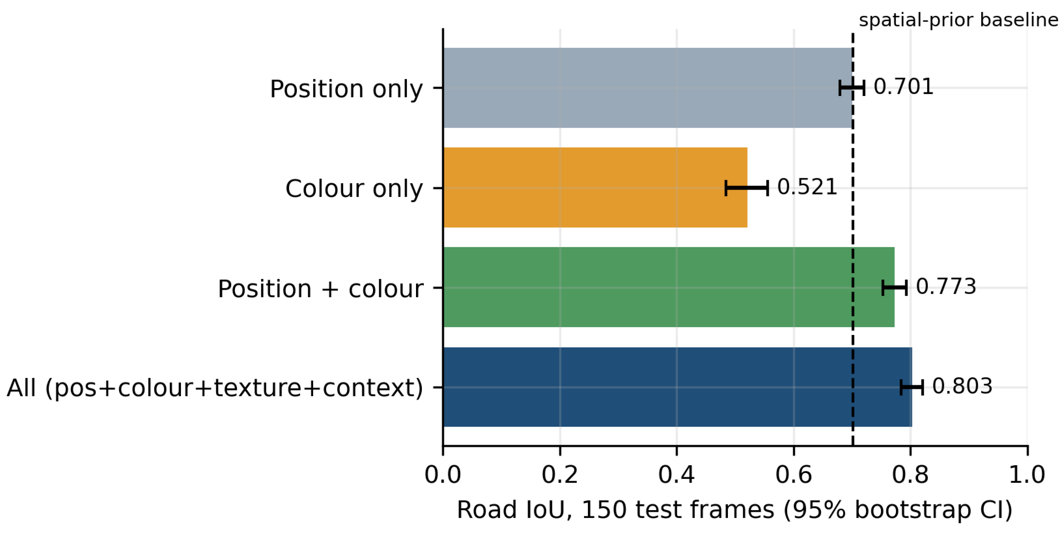
Figure 8.
Held-out segmentation examples (E3): input, ground truth, and predictions from position + colour and from all features.
Figure 8.
Held-out segmentation examples (E3): input, ground truth, and predictions from position + colour and from all features.
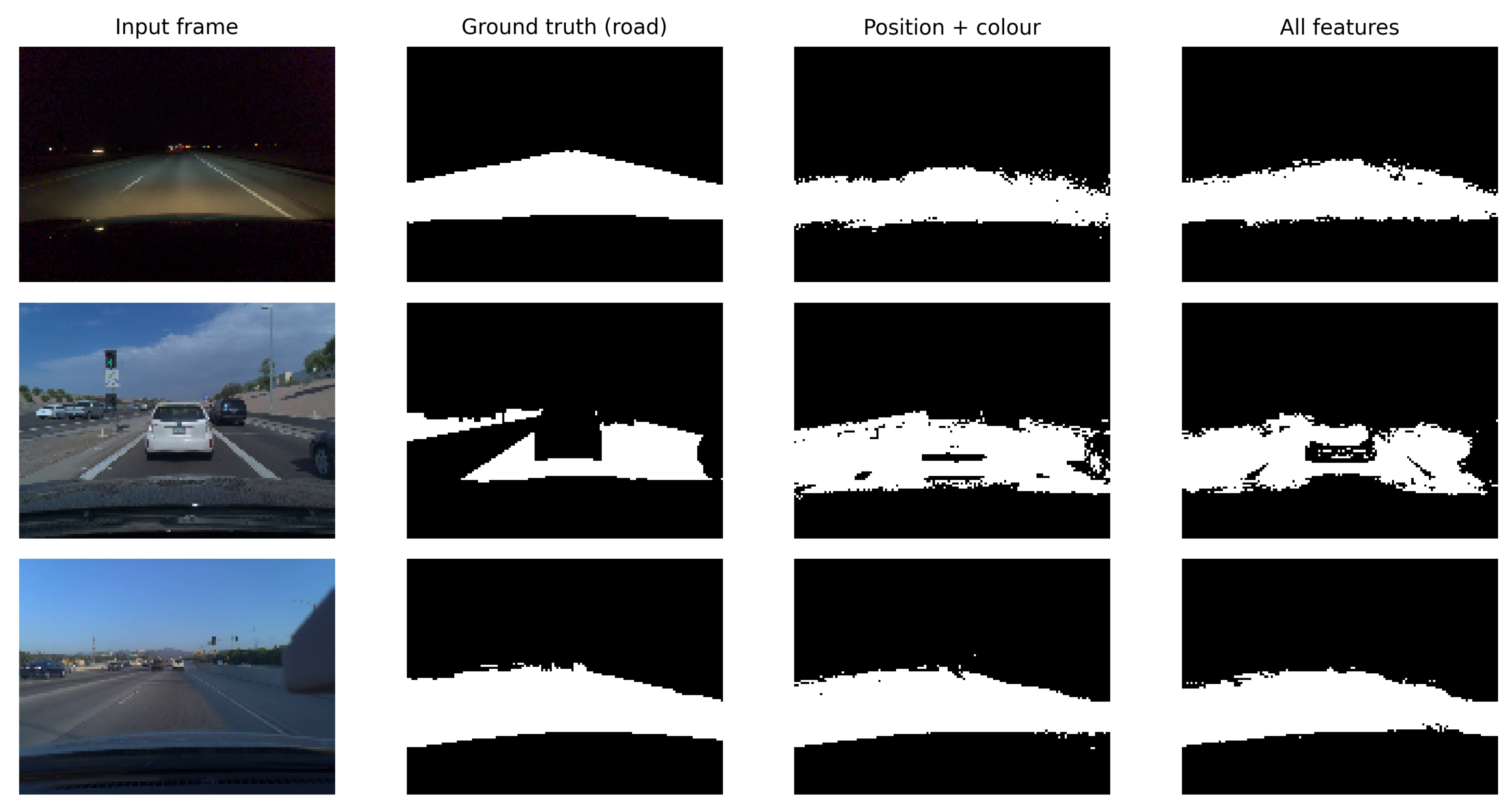
Figure 9.
Estimation architectures. (a) GNSS–odometry fusion filter of E5: odometry drives the prediction step, GNSS drives the update step through a switch that models the outage, and the baselines are shown dashed. (b) Localisation and mapping loop of E6: a selectable pose source (ground truth, odometry or landmark-corrected EKF) feeds the inverse sensor model and log-odds map update.
Figure 9.
Estimation architectures. (a) GNSS–odometry fusion filter of E5: odometry drives the prediction step, GNSS drives the update step through a switch that models the outage, and the baselines are shown dashed. (b) Localisation and mapping loop of E6: a selectable pose source (ground truth, odometry or landmark-corrected EKF) feeds the inverse sensor model and log-odds map update.
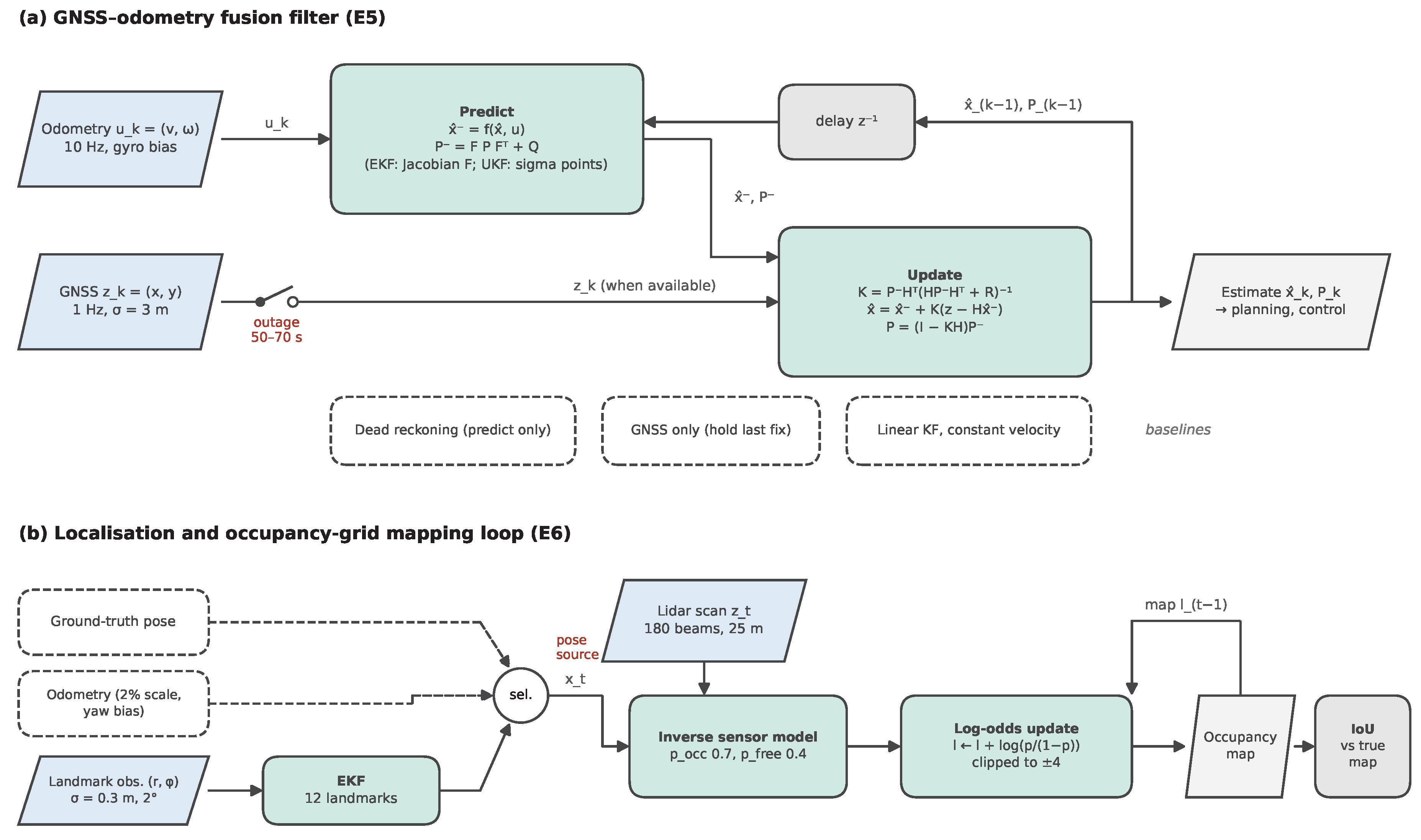
Figure 10.
GNSS–odometry fusion (E5). (a) Trajectories for run 0; the shaded segment marks the outage. (b) Position error over time (log scale).
Figure 10.
GNSS–odometry fusion (E5). (a) Trajectories for run 0; the shaded segment marks the outage. (b) Position error over time (log scale).
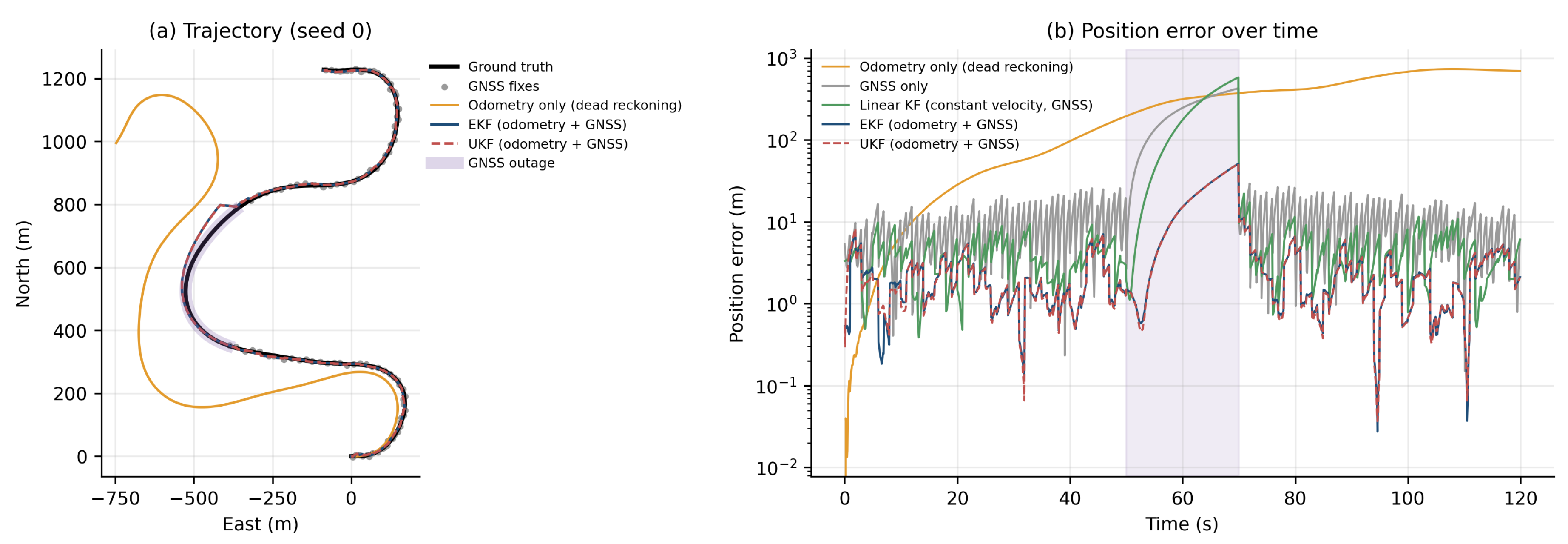
Figure 11.
Occupancy mapping (E6, seed 1). (a) World, landmarks and trajectories. (b–d) Maps from ground-truth, odometry and EKF poses with their occupied-cell IoU.
Figure 11.
Occupancy mapping (E6, seed 1). (a) World, landmarks and trajectories. (b–d) Maps from ground-truth, odometry and EKF poses with their occupied-cell IoU.
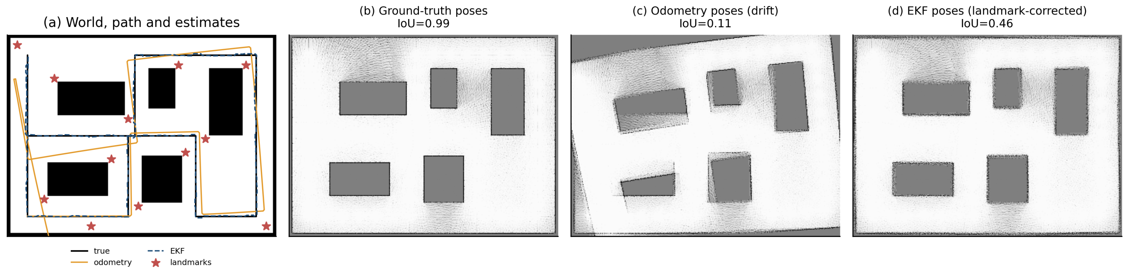
Figure 12.
Trajectory prediction pipeline of E7. All predictors receive the same pose-normalised history; four produce a single trajectory scored with ADE and FDE, and the library produces six hypotheses scored with and .
Figure 12.
Trajectory prediction pipeline of E7. All predictors receive the same pose-normalised history; four produce a single trajectory scored with ADE and FDE, and the library produces six hypotheses scored with and .
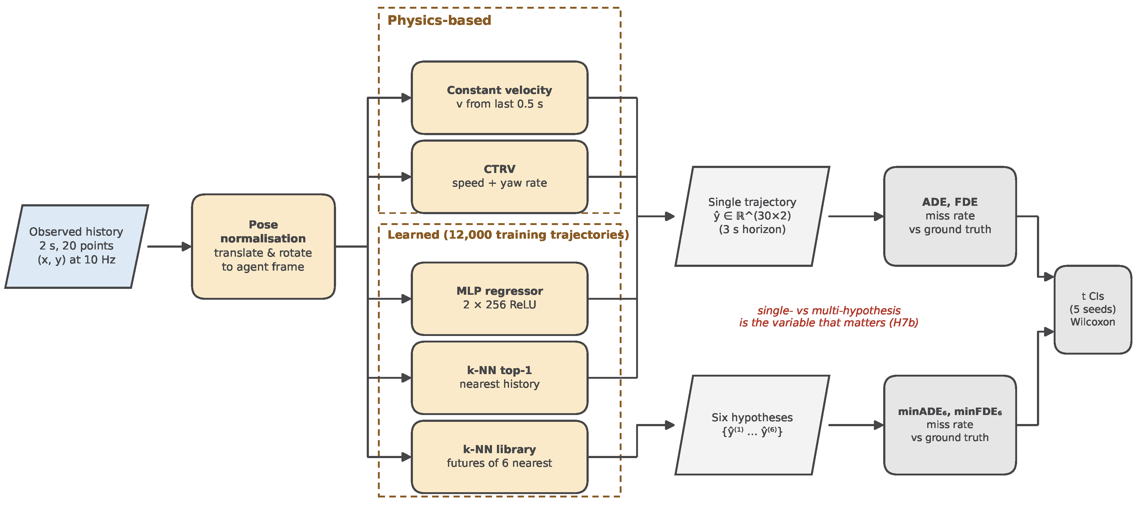
Figure 13.
Trajectory prediction (E7). (a) Mean ADE and FDE over five seeds. (b) ADE by manoeuvre. (c) A left turn with history, ground truth, single-output predictions and six library hypotheses.
Figure 13.
Trajectory prediction (E7). (a) Mean ADE and FDE over five seeds. (b) ADE by manoeuvre. (c) A left turn with history, ground truth, single-output predictions and six library hypotheses.
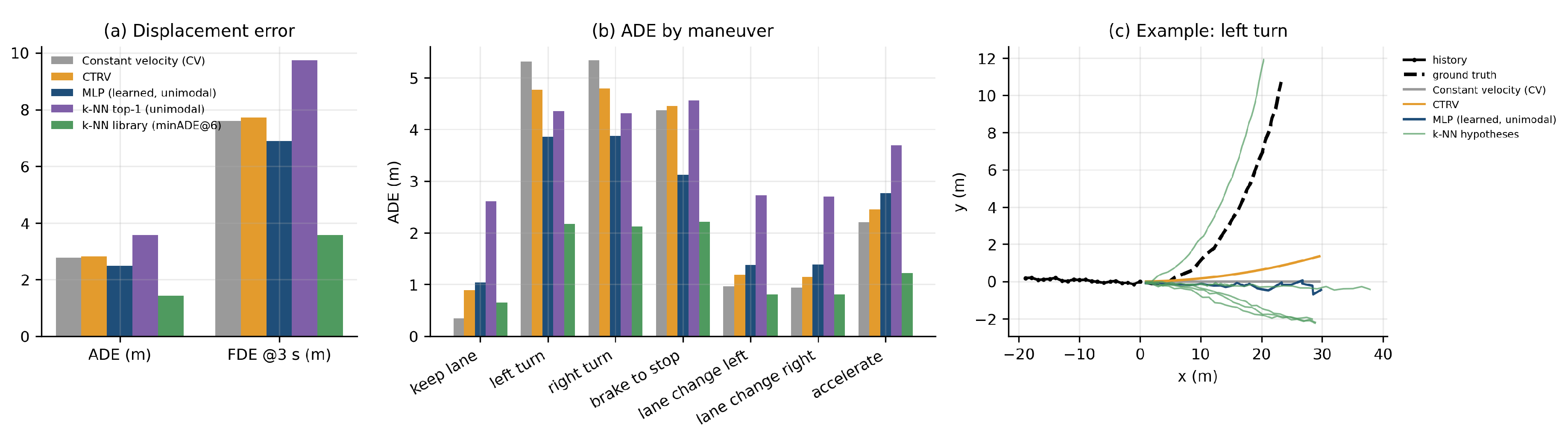
Figure 14.
A* search loop of E8, showing where the heuristic h and the weight enter the node ordering f = g + . Dijkstra’s algorithm is the special case h = 0.
Figure 14.
A* search loop of E8, showing where the heuristic h and the weight enter the node ordering f = g + . Dijkstra’s algorithm is the special case h = 0.
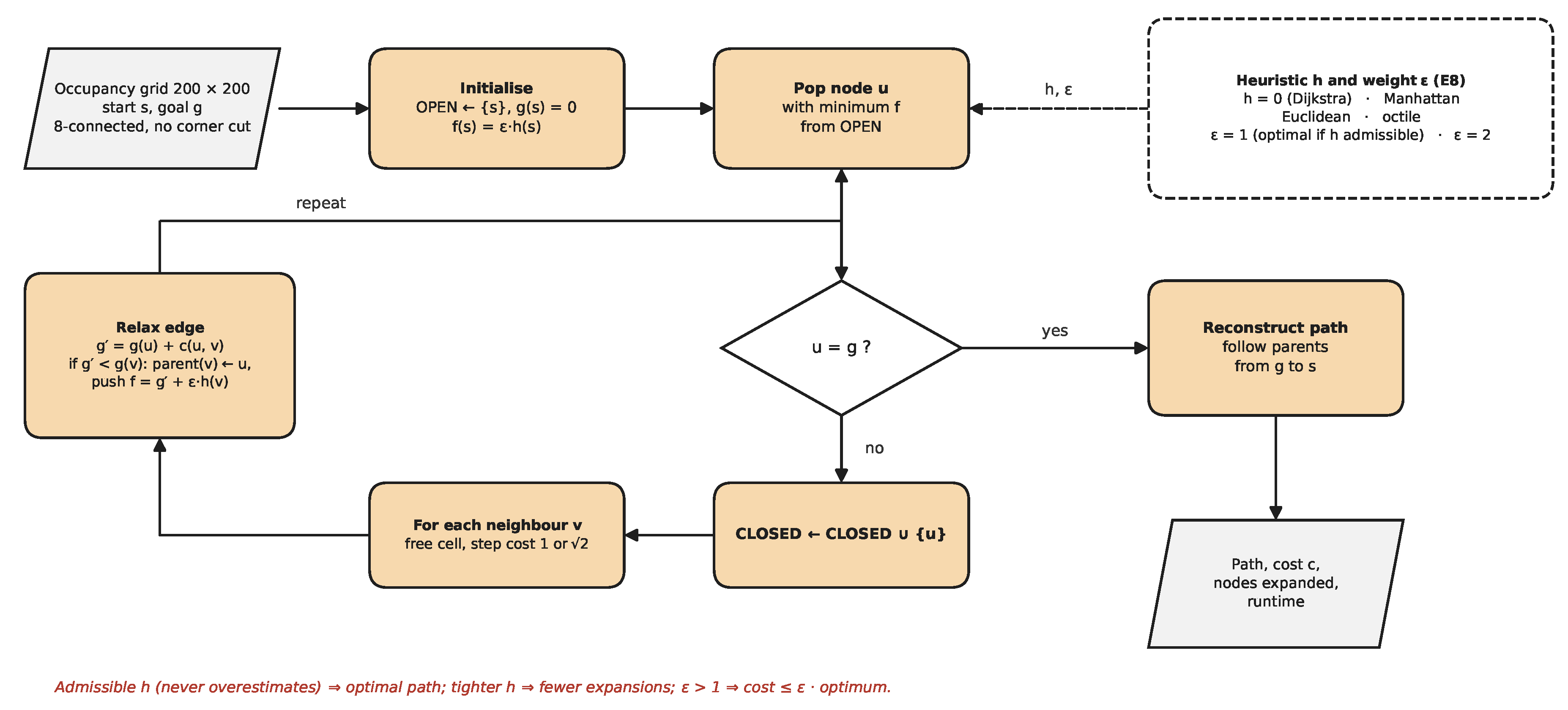
Figure 15.
Graph-search planning (E8). (a) Paths on one map. (b) Mean nodes expanded. (c) Runtime versus excess path cost.
Figure 15.
Graph-search planning (E8). (a) Paths on one map. (b) Mean nodes expanded. (c) Runtime versus excess path cost.
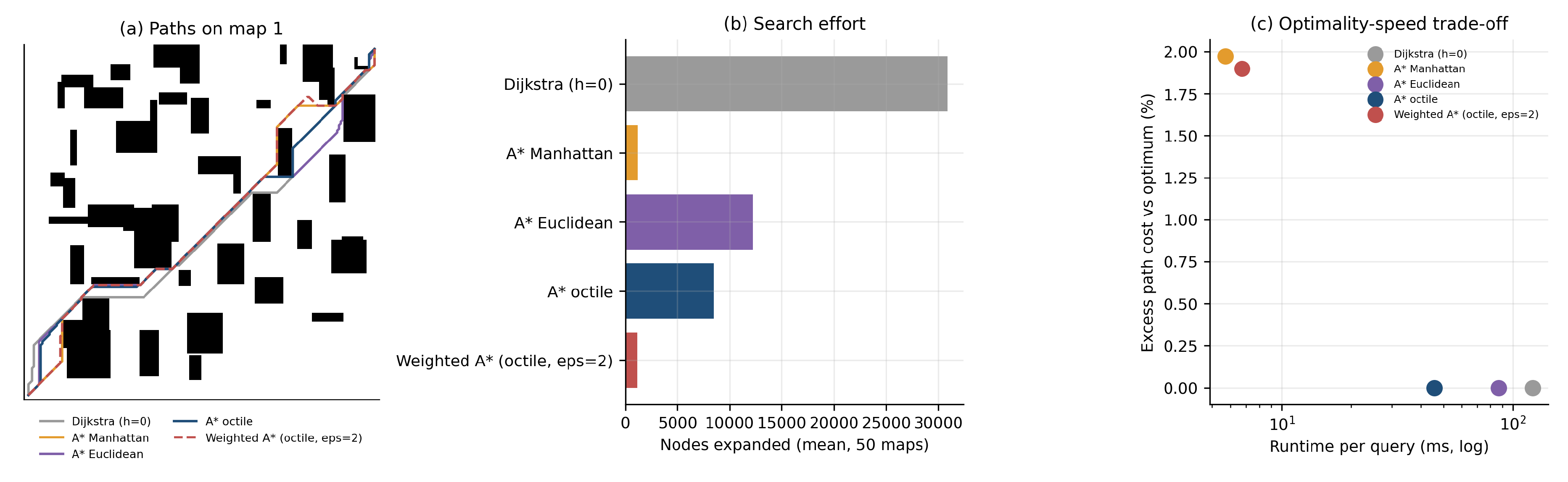
Figure 16.
Reinforcement-learning architecture of E9. Top: agent–environment training loop with state encoding, action selection and temporal-difference update. Bottom: evaluation of the frozen policy and three baselines on identical held-out traffic.
Figure 16.
Reinforcement-learning architecture of E9. Top: agent–environment training loop with state encoding, action selection and temporal-difference update. Bottom: evaluation of the frozen policy and three baselines on identical held-out traffic.
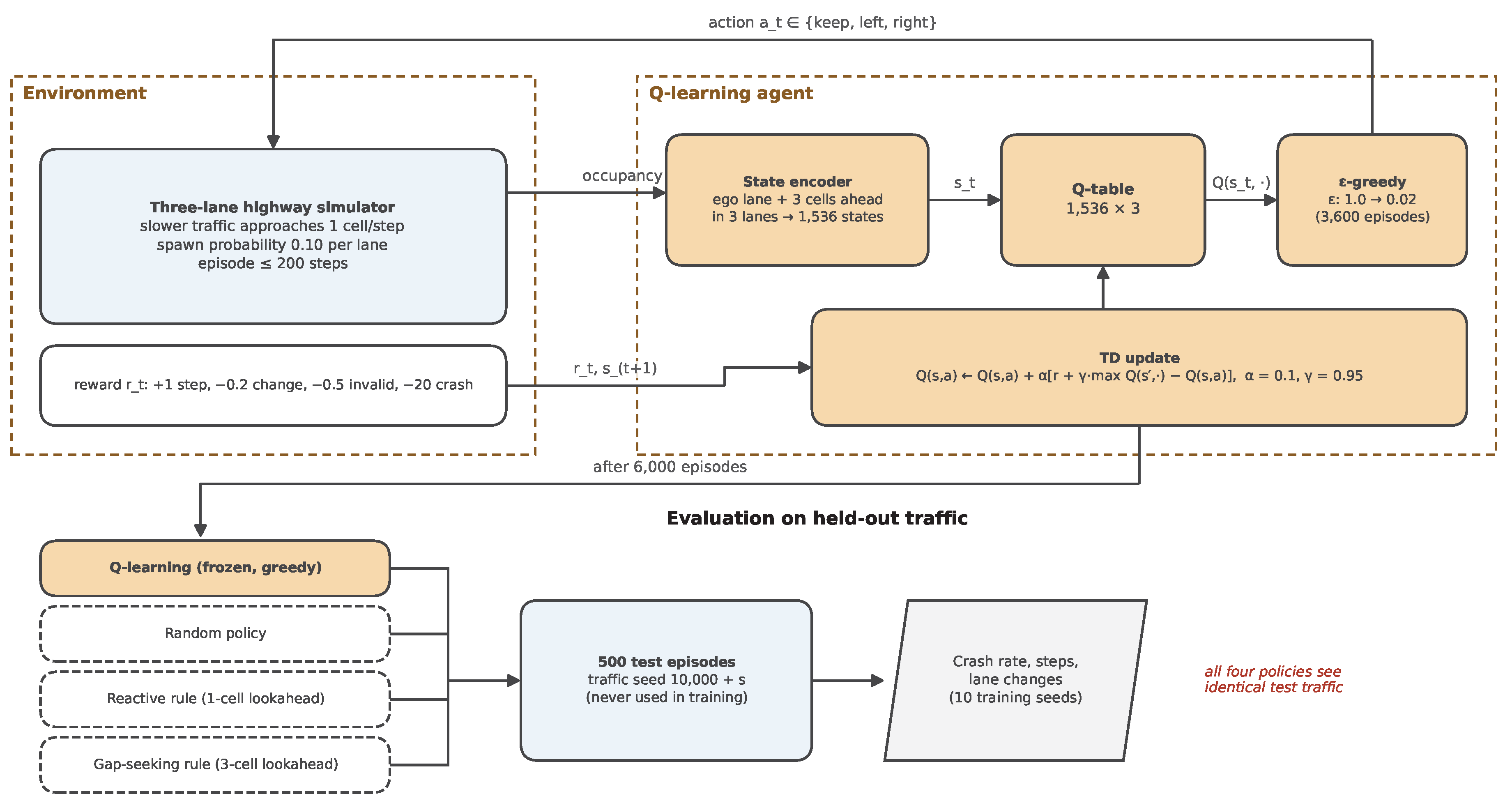
Figure 17.
Lane-change decisions (E9). (a) Training curve (seed 0). (b) Greedy crash rate during training (seed 0). (c) Test crash rate over 10 seeds with 95% CI.
Figure 17.
Lane-change decisions (E9). (a) Training curve (seed 0). (b) Greedy crash rate during training (seed 0). (c) Test crash rate over 10 seeds with 95% CI.
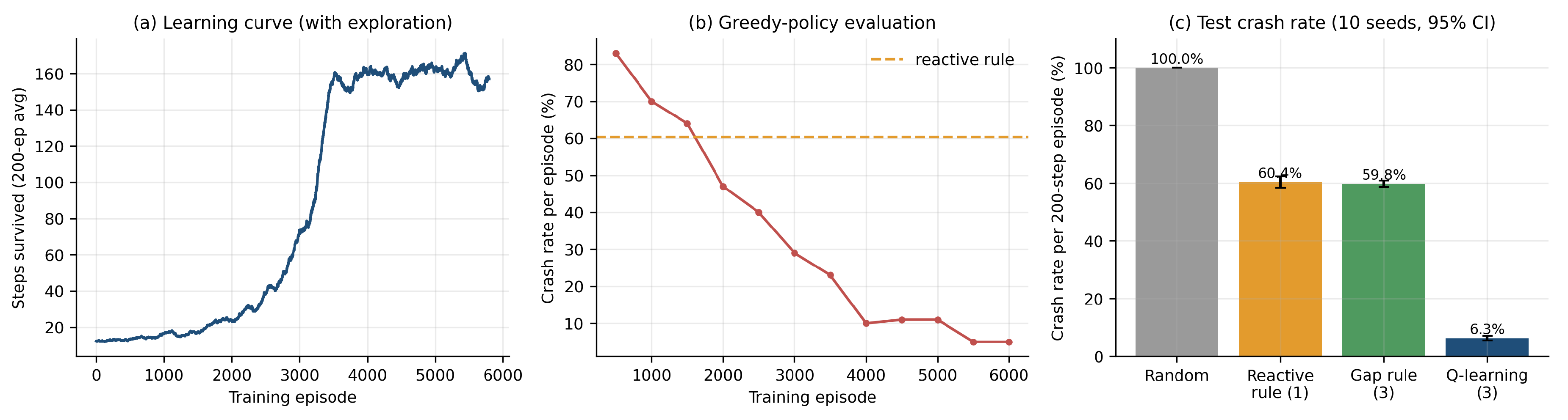
Figure 18.
Closed-loop path-tracking system of E10. The lateral controller acts on tracking errors, with curvature feed-forward for LQR and MPC; its command passes through saturation and a rate-limited actuator lag to the bicycle-model plant, and noisy pose measurements close the loop. The dashed outer loop selects each controller’s parameter on a separate validation path.
Figure 18.
Closed-loop path-tracking system of E10. The lateral controller acts on tracking errors, with curvature feed-forward for LQR and MPC; its command passes through saturation and a rate-limited actuator lag to the bicycle-model plant, and noisy pose measurements close the loop. The dashed outer loop selects each controller’s parameter on a separate validation path.
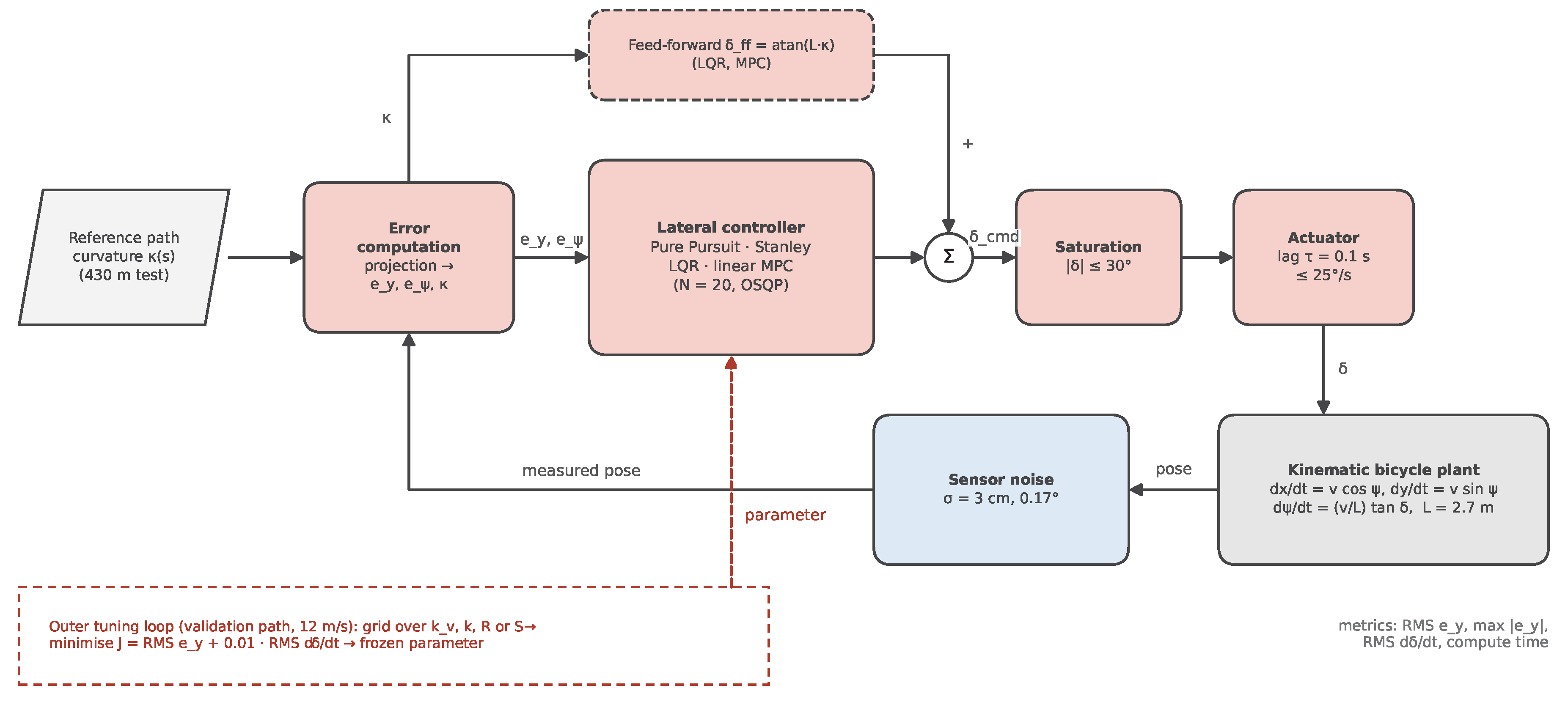
Figure 19.
Path tracking with validation-tuned controllers (E10). (a) Tracked paths at 15 m/s. (b) Lateral error along the path at 15 m/s (seed 0). (c) Mean RMS error at both speeds. (d) Accuracy versus computation at 15 m/s.
Figure 19.
Path tracking with validation-tuned controllers (E10). (a) Tracked paths at 15 m/s. (b) Lateral error along the path at 15 m/s (seed 0). (c) Mean RMS error at both speeds. (d) Accuracy versus computation at 15 m/s.
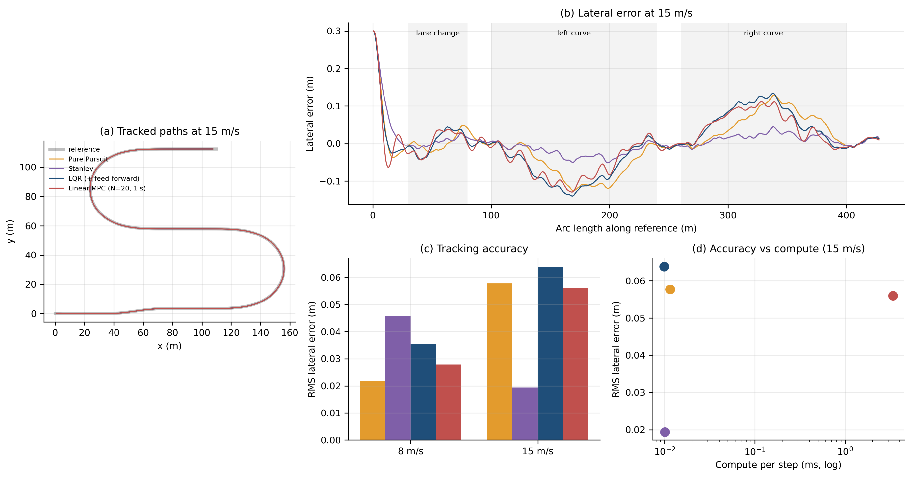
Figure 20.
Provenance of the field safety evidence in E11. Left: data produced and published by others (crash reports, benchmarks, testing reports). Right: the transcription and analyses performed in this study, and the tables and figures they produce.
Figure 20.
Provenance of the field safety evidence in E11. Left: data produced and published by others (crash reports, benchmarks, testing reports). Right: the transcription and analyses performed in this study, and the tables and figures they produce.
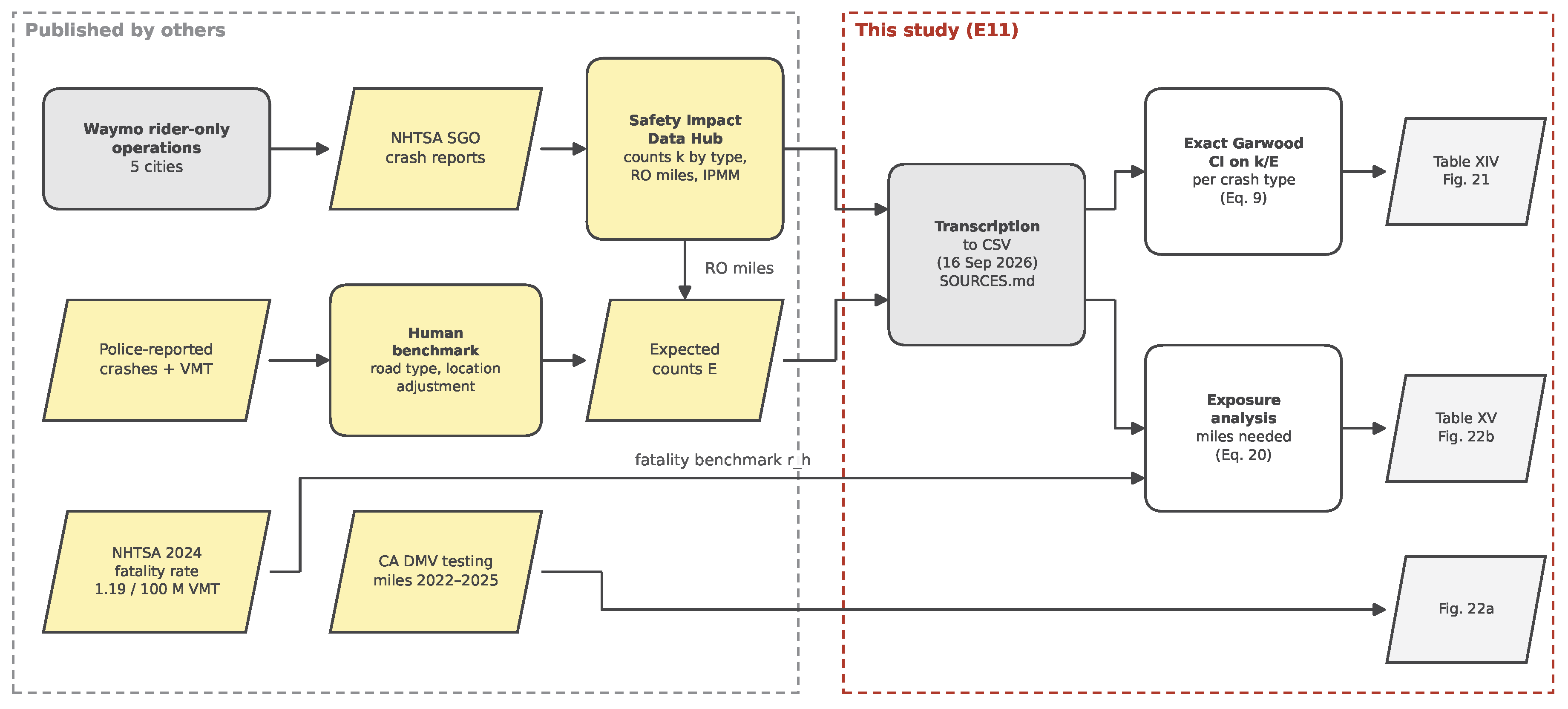
Figure 21.
Public safety data (E11). (a) Rider-only miles by city through March 2026. (b) Any-injury-reported crash rates versus human benchmarks. (c) Our re-analysis of observed/expected ratios by crash type with exact 95% CIs.
Figure 21.
Public safety data (E11). (a) Rider-only miles by city through March 2026. (b) Any-injury-reported crash rates versus human benchmarks. (c) Our re-analysis of observed/expected ratios by crash type with exact 95% CIs.
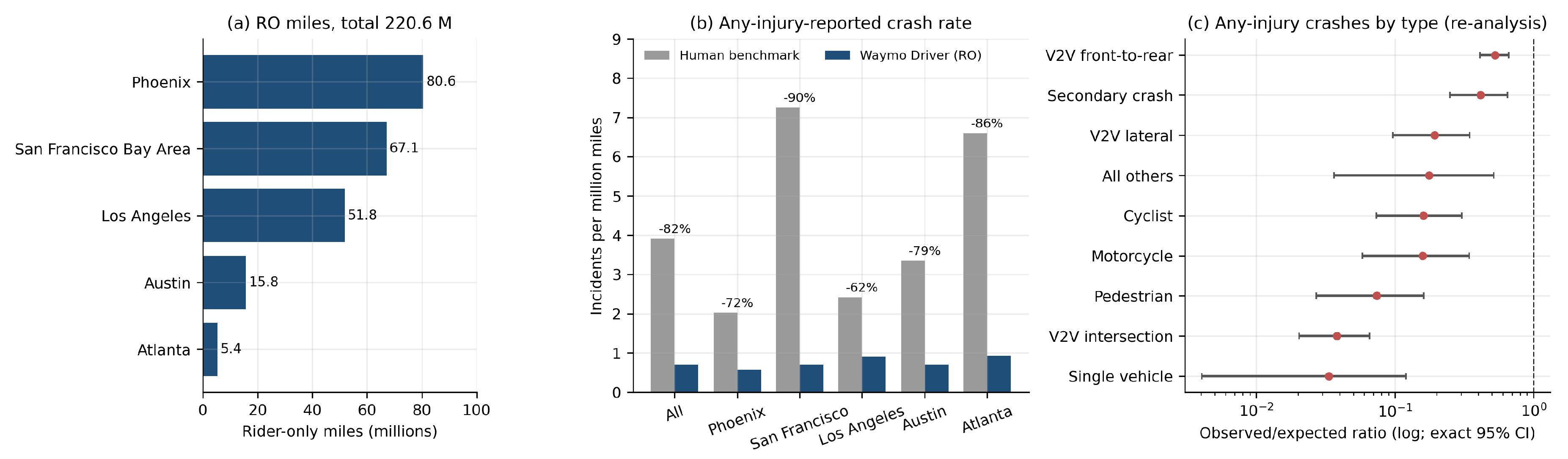
Figure 22.
(a) Autonomous testing miles reported to the California DMV; the 2024–2025 breakdown was not released. (b) Miles needed to demonstrate a reduction as a function of the true reduction; the dashed line marks cumulative rider-only miles.
Figure 22.
(a) Autonomous testing miles reported to the California DMV; the 2024–2025 breakdown was not released. (b) Miles needed to demonstrate a reduction as a function of the true reduction; the dashed line marks cumulative rider-only miles.
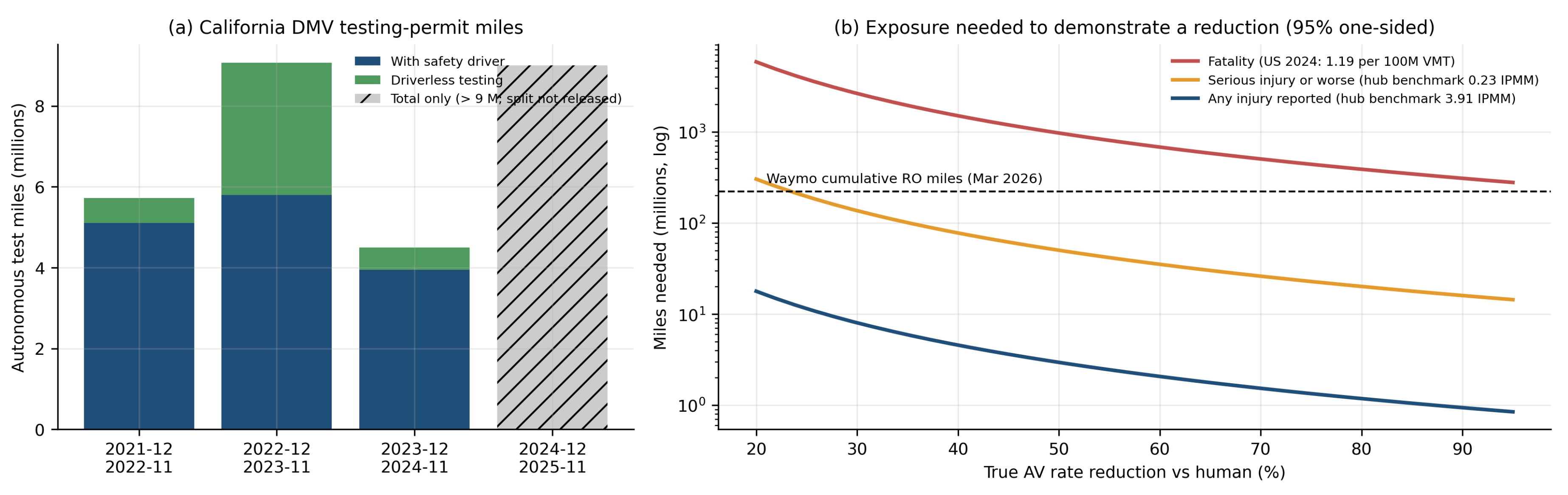
Figure 23.
Federated learning architecture of E12. Each vehicle trains on its own brightness-specific frames and exchanges only model weights with the server, which averages them (FedAvg). Centralised and local-only training are the comparison regimes; all models are evaluated on the same 150 test frames.
Figure 23.
Federated learning architecture of E12. Each vehicle trains on its own brightness-specific frames and exchanges only model weights with the server, which averages them (FedAvg). Centralised and local-only training are the comparison regimes; all models are evaluated on the same 150 test frames.
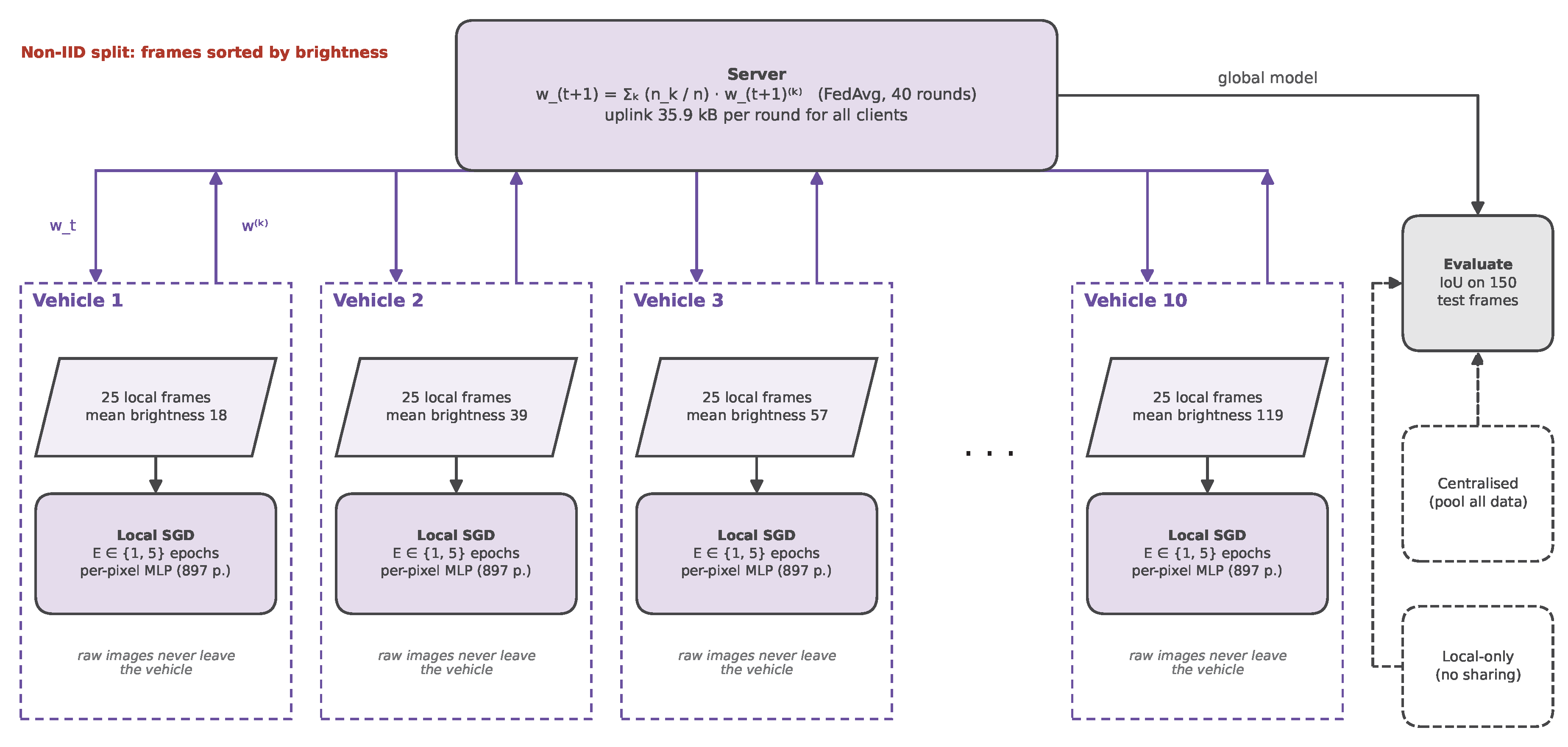
Figure 24.
Federated learning on real comma10k frames (E12). (a) Test IoU per round, averaged over five seeds. (b) Local-only IoU by client brightness compared with the shared and centralised models.
Figure 24.
Federated learning on real comma10k frames (E12). (a) Test IoU per round, averaged over five seeds. (b) Local-only IoU by client brightness compared with the shared and centralised models.
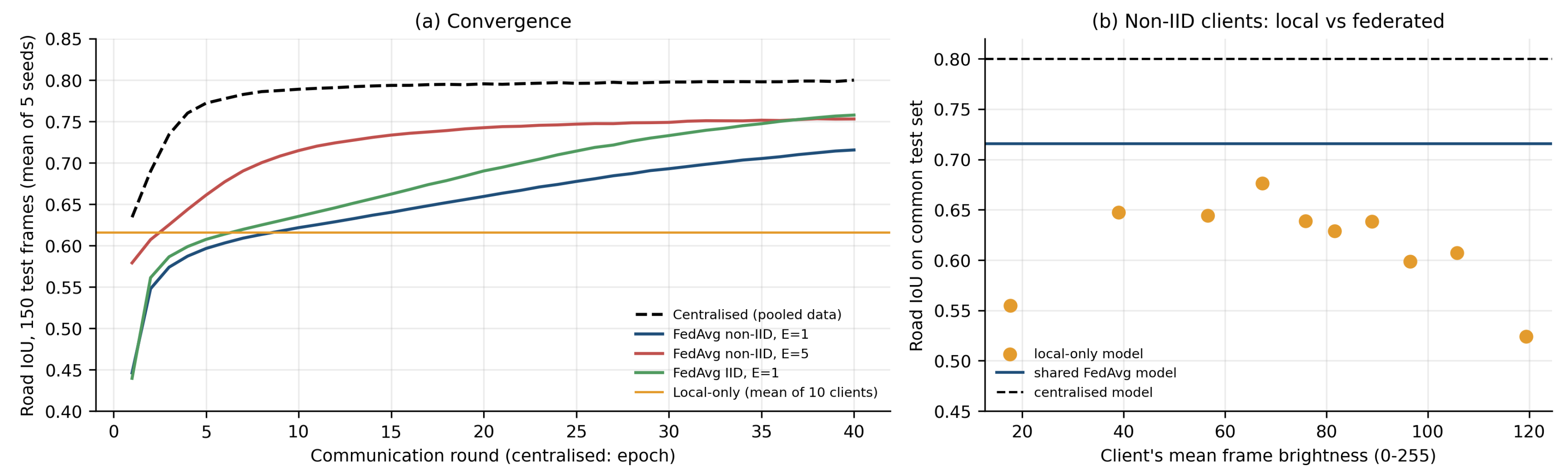
Figure 25.
Map from research questions to hypotheses, experiments and outcomes. Filled circles denote supported hypotheses, half-filled circles partly or practically supported ones, and open circles hypotheses that were not supported.
Figure 25.
Map from research questions to hypotheses, experiments and outcomes. Filled circles denote supported hypotheses, half-filled circles partly or practically supported ones, and open circles hypotheses that were not supported.
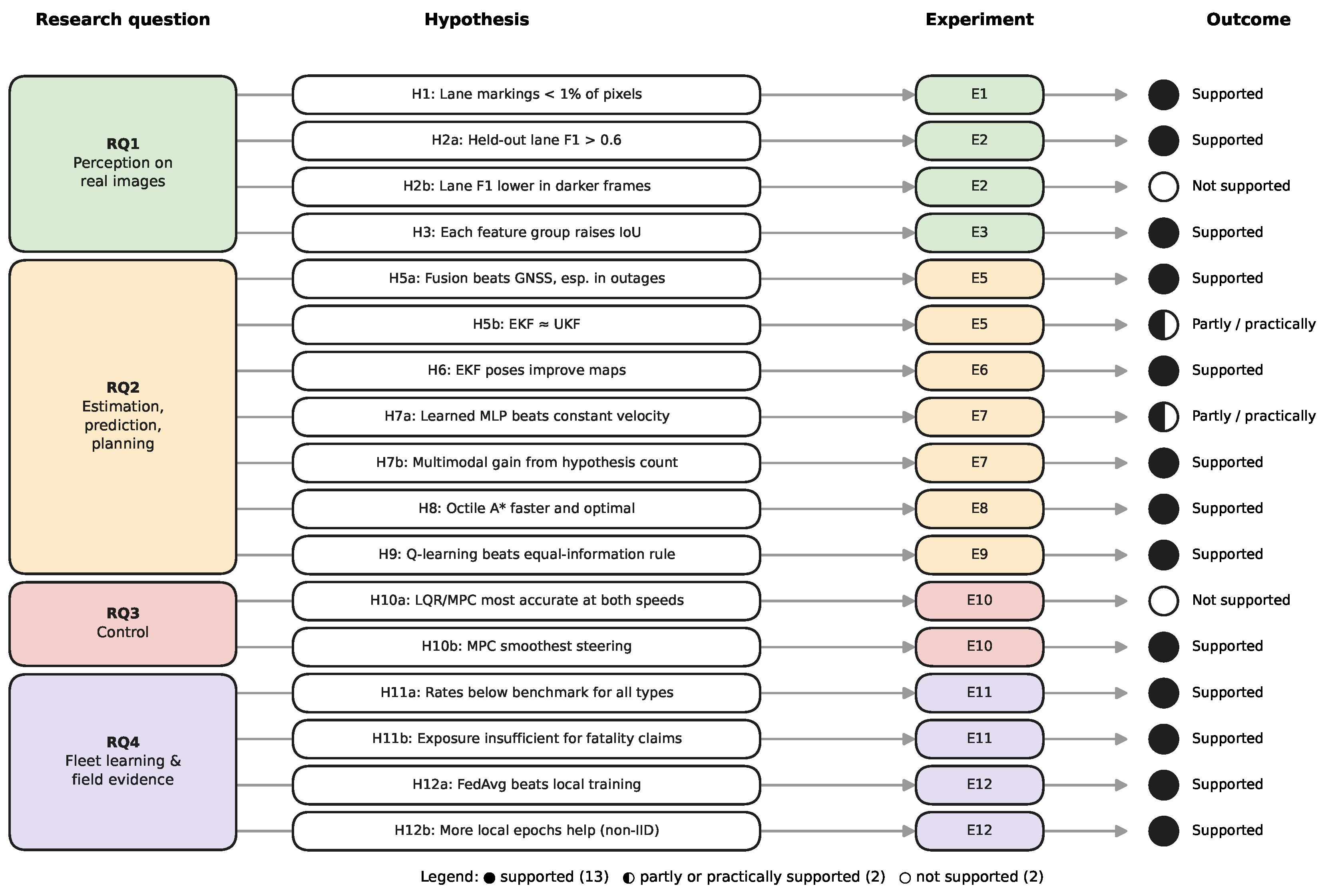
Disclaimer/Publisher’s Note: The statements, opinions and data contained in all publications are solely those of the individual author(s) and contributor(s) and not of MDPI and/or the editor(s). MDPI and/or the editor(s) disclaim responsibility for any injury to people or property resulting from any ideas, methods, instructions or products referred to in the content. |
© 2026 by the authors. Licensee MDPI, Basel, Switzerland. This article is an open access article distributed under the terms and conditions of the Creative Commons Attribution (CC BY) license (http://creativecommons.org/licenses/by/4.0/).
Copyright: This open access article is published under a Creative Commons CC BY 4.0 license, which permit the free download, distribution, and reuse, provided that the author and preprint are cited in any reuse.