

Submitted:
16 September 2026
Posted:
17 September 2026
You are already at the latest version
Abstract
Measuring multidimensional Quality of Life (QoL) increasingly relies on composite indicators to guide sustainable development policy. However, standard linear aggregation frameworks generally assume full compensability, allowing strong performance in one domain to mathematically mask severe deficits in another. For policymakers, this compensatory masking may conceal structural imbalances across sectors, obscuring localized vulnerabilities critical for targeted interventions. To address this diagnostic gap, we introduce the Sustainable Composite Indicator for Policy Evidence (SCIPE), a granular QoL assessment framework that explicitly penalizes horizontal imbalances across SDG-aligned dimensions. Using Bangladesh’s 64 administrative districts as a representative case study, we construct a multi-domain baseline that integrates traditional socio-economic metrics with satellite-derived night-time light data. SCIPE employs Principal Component Analysis (PCA) for data-driven indicator weighting and the Mazziotta-Pareto Index (MPI) to enforce an explicit variance penalty. Sensitivity analysis against the Human Development Index (HDI) confirms convergent validity while demonstrating SCIPE’s sensitivity to inter-sectoral volatility. Empirical findings reveal that penalizing horizontal variance significantly reconfigures district rankings: rewarding balanced developmental trajectories while exposing hidden trade-offs, such as ecological and public health deficits within affluent industrial corridors. Ultimately, this study demonstrates that aggregation choices fundamentally dictate policy interpretation, underscoring the necessity of evaluating balanced progress rather than relying solely on macro-level averages.
Keywords:
quality of life
; composite indicators
; SDGs
; non-compensatory aggregation
; sub-national development
1. Introduction
The measurement of national progress has shifted over the past few decades, moving away from strictly monetary aggregates like Gross Domestic Product (GDP) toward multidimensional frameworks of human well-being [37]. Economic growth does not automatically result in equal social progress for everyone. To operationalize a broader vision of sustainable development, policymakers increasingly rely on Composite Indicators (CIs). By synthesizing diverse socio-economic, environmental, and infrastructural metrics into unified scores, CIs serve as tools for monitoring multidimensional targets such as the Sustainable Development Goals (SDGs) [18,34].
While these multidimensional frameworks offer conceptual advantages, their standard mathematical execution typically relies on the assumption of full compensability. The standard practice in index construction, common in frameworks like the early Human Development Index (HDI), is to aggregate diverse developmental domains using simple or weighted linear averages. Mathematically, this property implies that a deficit in one area of human life can be offset, or compensated for, by high performance in another [38]. This design is effective for evaluating average achievement across a region. However, it is less equipped to capture structural imbalances among distinct developmental sectors.
Within the context of sub-national governance, this compensatory logic alters how regional assessments are interpreted. It establishes a paradigm where a district experiencing environmental degradation or strained public health systems can still achieve an elevated overall quality of life ranking if its economic or infrastructural output is sufficiently large. For local administrators and national planners, this averaging approach can introduce a masking effect, blending disparate sector scores and potentially obscuring structural imbalances. Consequently, asymmetrical development may be interpreted as balanced progress. If an objective of sustainable development monitoring is to evaluate the uniformity of performance across all dimensions, a composite index can benefit from explicitly highlighting these localized vulnerabilities rather than averaging them out.
To complement existing assessment methods, this article proposes the Sustainable Composite Indicator for Policy Evidence (SCIPE). Using Bangladesh as a representative case study of regional development, we construct a district-level Quality of Life index across five SDG-aligned domains: Health, Education, Infrastructure, Environment, and Living Conditions. Rather than evaluating average achievement alone, SCIPE implements a non-compensatory aggregation approach. Utilizing the Mazziotta-Pareto Index (MPI) framework, our methodology applies a mathematical penalty for horizontal imbalance across domains [16]. This ensures that districts with symmetrical progress maintain their relative standings, while those with deep sectoral deficits receive a corresponding penalty.
To illustrate the diagnostic flaw of compensatory masking, consider two stylized administrative regions evaluated across five development domains on a normalized scale [0, 1]:
- District A (Balanced Trajectory): Exhibits uniform, intermediate progress across all domains: Living Conditions (0.60), Health (0.60), Education (0.60), Infrastructure (0.60), and Environment (0.60).
- District B (Asymmetrical Industrial Hub): Displays accelerated infrastructure and living conditions driven by rapid industrialization, but experiences severe ecological and public health degradation: Living Conditions (0.95), Infrastructure (0.90), Education (0.60), Health (0.40), and Environment (0.15).
Under standard linear aggregation (arithmetic mean), both districts achieve an identical composite score of 0.600 (RankA = RankB). This mathematical equivalence creates a critical policy blind spot: it suggests that District B’s rapid industrialization successfully offsets its acute environmental and public health vulnerabilities. In contrast, the proposed SCIPE framework explicitly penalizes horizontal variance across domains. While District A incurs zero penalty (A = 0.000) and maintains its score of 0.600, District B’s high sectoral dispersion (B = 0.302) triggers an explicit penalty, reducing its non-compensatory score to 0.298 (0.600–0.302). This differentiation exposes localized vulnerabilities, ensuring that regional planners are alerted to structural imbalances rather than misled by composite averages.
By shifting the focus from maximizing average performance to evaluating regional balance, this paper presents an alternative perspective for evidence-based policy formulation. Our contributions are threefold:
- We construct a baseline framework for granular Quality of Life measurement centered on Bangladesh, combining traditional socio-economic surveys with remotely sensed geospatial data to capture local realities under data constraints.
- We implement a non-compensatory aggregation approach that accounts for horizontal imbalance across development domains, offering an alternative to traditional linear indices.
- Through empirical demonstrations and localized case studies, we show how accounting for imbalance reorders regional rankings, exposing trade-offs—such as the tension between rapid infrastructural expansion and environmental conditions—that standard averaging methods may leave undetected.
The remainder of this manuscript is organized as follows: Section 2 reviews relevant literature on composite indicator construction and the compensability problem. Section 3 outlines the materials, data sources, and indicator mapping. Section 4 details the non-compensatory methodology, workflow architecture, and mathematical formulation of SCIPE. Section 5 presents the empirical results and sub-national spatial distributions across the 64 districts of Bangladesh, our representative case study. Section 6 discusses developmental synergies and trade-offs, evaluates compensatory masking through rank-shift analysis, and presents a targeted policy optimization simulation. Section 7 provides comprehensive statistical and spatial validation, including formative reliability assessments, external benchmarking, and sensitivity analyses. Finally, Section 8 provides concluding remarks, operational merits, limitations, and future research directions.
2. Literature Review
This section contextualizes the methodological evolution of Quality of Life (QoL) indices, examining the mathematical assumptions underlying their construction and highlighting associated constraints.
2.1. The Evolution of Quality of Life Measurement
The measurement of national progress has historically been dominated by economic aggregates, most notably Gross Domestic Product (GDP). However, GDP’s inability to capture holistic well-being, non-market labor, and environmental sustainability has been extensively critiqued [4,8]. To address this dimensional narrowness, global institutions shifted toward Composite Indicators (CIs) capable of synthesizing diverse socio-economic and environmental metrics into unified scores [18].
Foundational efforts such as the Physical Quality of Life Index (PQLI) [17] and the Human Development Index (HDI) [27] established the standard for multidimensional measurement by integrating life expectancy, education, and income. Building on this, the Multidimensional Poverty Index [1] further disaggregated welfare to capture localized household deprivations. While these indicators facilitate cross-regional comparisons, their construction necessitates a rigorous assessment to avoid misleading policy conclusions regarding country performance [5]. Despite these advancements, a significant gap persists in representing the status of granular regions inherent in traditional reporting.
National-level statistics frequently suffer from geographic masking, where high-performing urban centers artificially inflate national averages, thereby obscuring regional disparities [13]. This reliance on macro-aggregates creates a blind spot for policymakers; a nation may appear to be on a trajectory of steady growth while simultaneously obscuring regional variations in environmental or social conditions. Addressing this masking effect has become a central objective for contemporary governance; for instance, the Government of Bangladesh has explicitly prioritized multidimensional assessments and regional equity in its latest strategic reviews to monitor progress toward the 2030 Agenda [6]. However, Bangladesh represents a context where the success of the 2030 Agenda is tied to the alignment of governance with measurable institutional performance [20]. This domestic shift reflects a broader global research frontier in the governance of Sustainable Development Goals (SDGs), which increasingly calls for regional monitoring frameworks to bridge the gap between high-level sustainability targets and their practical, sub-national implementation [9].
To resolve this granularity gap, recent advancements in the spatial domain have expanded these frameworks, integrating geospatial data and satellite proxies to map well-being at the district level [24,25]. These remote-sensing techniques have been empirically validated as proxies for economic and infrastructure asset distribution, particularly within the rural administrative zones of low- and middle-income countries [19]. Transitioning from national to sub-national statistics is not merely a matter of resolution, but of diagnostic granularity. Granular mapping allows for the detection of spatial heterogeneity—the reality that development is not uniform but clusters and exhibits spatial dependencies linked to local geographic and infrastructural conditions [33]. However, while the inputs to these indices have become increasingly sophisticated, the mathematical mechanisms used to aggregate them often rely on linear averaging techniques that implicitly assume full compensability across domains. This structural property may obscure localized, domain-specific policy realities, motivating the exploration of non-compensatory frameworks.
2.2. Methodological Limitations of Full Compensability
The central debate in CI construction revolves around the choice of aggregation technique, which dictates the compensability among the domains of the index. Mathematically, compensability dictates the extent to which a deficit in one domain can be offset by a surplus in another [38].
The vast majority of legacy indices employ Linear Aggregation. Calculated as the weighted or simple arithmetic mean of normalized indicators, this approach is mathematically straightforward and assumes full compensability. In development literature, this logic strictly aligns with the paradigm of “weak sustainability”, which assumes that fundamental natural or social capital can be substituted with manufactured capital. Under a linear framework, a deficit in environmental protection or public health can be offset by high economic output or infrastructural density. As highlighted by [22], different aggregation choices significantly alter conclusions about well-being. For regional policymakers, linear compensability can introduce a compensatory masking effect, allowing highly unbalanced development to be interpreted as uniform advancement.
To evaluate sectoral balance alongside overall achievement, researchers explore partial or non-compensatory methods. The recognition of this methodological boundary is well-documented; notably, the UNDP shifted the HDI from an arithmetic to a geometric mean in 2010 specifically to limit these full compensabilities across dimensions [21]. Geometric aggregation, which utilizes the product of indicators, partially restricts compensability by penalizing scores when any single domain approaches zero [18]. However, for rigorous socio-economic monitoring where fundamental domains are considered strictly non-substitutable, reflecting “strong sustainability”, geometric averaging offers only a partial adjustment. While it penalizes scores approaching zero, it mathematically continues to permit substitutability at intermediate values and fails to directly penalize the internal variance (inequality) between domains. Consequently, explicit penalty functions offer an alternative approach for evaluating balanced development.
2.3. The Mazziotta-Pareto Index and Penalty Functions
To evaluate balanced progress alongside overall achievement, Mazziotta and Pareto [16] proposed a non-compensatory approach that explicitly penalizes horizontal variability. The Mazziotta-Pareto Index (MPI) adjusts the arithmetic mean of a unit’s scores by subtracting a penalty relative to the standard deviation of its domain values.
Unlike Multi-Criteria Decision Making (MCDM) methods such as TOPSIS, which require the definition of theoretically ideal benchmarks [11], the MPI calculates penalties based purely on internal data variance. This ensures that regions exhibiting balanced development across all dimensions are rewarded, while those exhibiting extreme internal disparities face an explicit mathematical penalty.
2.4. Data-Driven Weighting and Indicator Harmonization
Before non-compensatory aggregation can occur, the underlying indicators must be standardized and weighted. While subjective weighting techniques, such as the Analytic Hierarchy Process [23], allow for expert input, they inherently introduce human bias. Consequently, recent methodological standards frequently favor data-driven approaches to ensure objective evaluation [15]. Principal Component Analysis (PCA) is widely utilized to derive weights by capturing the maximum variance within the dataset, ensuring that highly correlated indicators do not redundantly inflate the index [14]. By coupling PCA weighting with Z-score or Min-Max normalization, an index establishes a statistically neutral foundation before applying a non-compensatory penalty [7].
The proposed SCIPE framework adopts this sequence: applying data-driven PCA weighting to standardized domain scores, and subsequently utilizing the Mazziotta-Pareto approach to penalize unbalanced regional development.
3. Materials and Data Architecture
Transitioning from the theoretical critiques established in the literature to an empirical application, this study operationalizes a new indicator entitled Sustainable Composite Indicator for Policy Evidence (SCIPE) using Bangladesh as a representative case study. As a low-resource nation experiencing rapid, yet geographically uneven, economic and infrastructural growth [30], Bangladesh provides a highly relevant context to test the effects of compensatory masking. To ensure this framework is grounded in robust, verifiable inputs, we utilize curated datasets that comprehensively cover the nation’s 64 administrative districts. This section outlines the primary data repository and the selection of the five fundamental developmental domains required to construct and compute the SCIPE index.
3.1. Data Repository and Resolution
The primary data for the SCIPE framework is sourced from the Bangladesh Quality of Life (BDQOL) repository (https://bdqol.dndlab.org/). Functioning as a secure, offline-curated database, BDQOL harmonizes heterogeneous data sources, ranging from traditional census statistics (e.g., the Household Income and Expenditure Survey) to non-traditional spatial data (e.g., satellite-derived nighttime luminosity). This remote sensing layer can serve as an objective spatial proxy for physical infrastructure distribution in contexts where localized survey data is updated infrequently [30].
An essential operational consideration of the SCIPE framework is its cost-effectiveness and practical feasibility in low-resource and developing settings. Classical sub-national welfare assessments rely almost exclusively on primary household sample surveys (e.g., HIES, DHS). While statistically rigorous, conducting nationwide door-to-door enumeration involves massive logistical overhead, budgets exceeding millions of USD, and extended bureaucratic lag [30].
To enhance spatial and infrastructural granularity without introducing additional financial burdens, SCIPE incorporates non-traditional data (e.g., satellite-derived night-time luminosity and environmental sensor estimates for ambient PM2.5). The primary objective is to synthesize multi-source information for a more granular view of sub-national disparities; here, non-traditional data serves not as an indispensable requirement, but as an accessible, cost-effective proxy to augment sparse administrative data.
Crucially, these earth observation repositories are globally open-access, continuously updated, and completely free of charge through public archives (such as NASA, NOAA, and academic open repositories). Furthermore, all spatial zonal statistics, directional alignments, and aggregation algorithms are implemented using standard open-source Python (version 3.8) toolkits (rasterio, geopandas, and scikit-learn). Consequently, integrating non-traditional spatial proxies introduces zero marginal data acquisition cost and requires no proprietary software licensing, significantly reducing the overall cost of sub-national diagnostics compared to classical survey-only approaches.
By aligning all collected metrics to the 64 administrative districts of Bangladesh, the repository resolves spatial mismatches between different national agencies. This standardizes the spatial resolution at the exact jurisdictional level where local government budgets are drafted and policy interventions are executed. The reliance on this harmonized repository ensures that our computational index is built upon a spatially consistent baseline using aligned administrative data sources.
Alongside spatial standardization, constructing a multi-source diagnostic framework in data-scarce settings requires addressing temporal synchronization across asynchronous survey cycles. In low- and middle-income countries, comprehensive household economic surveys (HIES), demographic and health surveys (DHS), and official statistical yearbooks are conducted at multi-year intervals rather than annual cadences. Integrating these authoritative national benchmarks alongside recent satellite- and sensor-based data proxies establishes a synthetic cross-sectional structural baseline [18,30]. This temporal synthesis is methodologically sound for two reasons:
- Uniform Intra-Indicator Synchronization: Every underlying indicator was enumerated simultaneously across all 64 districts within its respective survey cycle (e.g., DHS 2014 or HIES 2016 sampled all districts in the same period). Consequently, cross-district variance and rank ordering reflect spatial disparities rather than staggered measurement timing across jurisdictions.
- Structural Inertia of Macro-Development: The core dimensions captured—such as childhood stunting, regional poverty patterns, paved road density, forest reserves, and geophysical hazard exposure—represent slow-moving, path-dependent structural endowments that evolve over decadal horizons rather than fluctuating erratically year-to-year.
Therefore, while the resulting framework functions as a stationary structural baseline rather than a high-frequency tracking monitor, it possesses the diagnostic capacity to identify spatial inequalities and cross-sectoral trade-offs across a country’s sub-national administrative regions.
3.2. Definition of Domain Variables and Indicator Directionality
To capture the multidimensional nature of regional development without inflating the index with redundant variables, we structured the framework around five core domains: Living Conditions, Health, Education, Infrastructure, and Environment. These domains were explicitly selected to reflect the fundamental pillars of societal progress. Living Conditions, Health, and Education capture human capital and basic welfare, while Infrastructure and Environment represent the physical and ecological systems required to support and maintain long-term development.
By consolidating the 17 United Nations Sustainable Development Goals (SDGs) [28,34] into these five focused domains, this framework simplifies the high dimensionality of global objectives into localized, actionable administrative categories that align with the organizational mandates of the regional ministries. However, it is necessary to define the methodological boundaries of this mapping. While SCIPE successfully captures the majority of the 2030 Agenda, certain global targets, specifically SDGs 5, 10, 12, 14, and 17, were intentionally excluded from the current framework. Goals that inherently measure macro-level international cooperation (e.g., SDG 17: Partnerships for the Goals), or dimensions that currently lack robust, uniformly disaggregated data at the district level, cannot be mathematically integrated into a highly granular spatial index without introducing imputation bias. Consequently, the chosen domains represent a data-verifiable subset of the SDGs optimized for localized policy intervention.
A requirement for constructing a sustainable composite index is ensuring that the framework accurately differentiates between developmental achievements and indicators of societal decay across regions. To synthesize these diverse domains into a single, cohesive metric, we populated each domain with specific, representative socio-economic indicators. Conceptually, while a domain represents a broad, abstract dimension of development (e.g., Health), an indicator acts as a quantifiable proxy used to capture a distinct facet of that dimension (e.g., Under-5 Mortality Rate). However, before these indicators can be aggregated, the raw data must be mathematically harmonized. Because these indicators inherently operate with different polarities concerning human well-being, establishing clear mathematical directionality for every underlying variable is necessary. This ensures the index can evaluate regional performance without mathematical contradictions. Based on this inherent polarity, the selected indicators within our framework are classified as follows:
- Positive Indicators (+): Metrics where a higher value signifies a superior standard of living (e.g., Per Capita Income, Paved Roads). These are retained in their original scale during preprocessing.
- Negative Indicators (−): Metrics where a higher value signifies societal vulnerability or degradation (e.g., Extreme Poverty Rate, Air Quality PM2.5). These require mathematical inversion prior to aggregation to ensure that a higher composite score consistently represents a better quality of life.
To provide full transparency on this structural mapping, Table 1 details the specific indicators selected to represent each domain, their respective sources, and their alignment with the Global Indicator Framework for the Sustainable Development Goals [28,34], alongside their explicit mathematical directionality.
4. Methodology and SCIPE Framework Formulation
To construct a multidimensional indicator, this study applies a multi-stage statistical framework. Moving away from subjective expert weighting and linear averages, we adopt an objective, data-driven, and non-compensatory methodology. The formulation of the SCIPE index systematically follows three primary mathematical steps: data preprocessing, data-driven weighting via Principal Component Analysis (PCA), and non-compensatory aggregation using the Mazziotta-Pareto Index (MPI).
4.1. Computational Methodology of the SCIPE Framework
To provide a clear overview of the data-processing and aggregation architecture, the end-to-end computational pipeline of the SCIPE framework is illustrated in Figure 1. The workflow is organized into five sequential stages: multi-source data ingestion, directional and scale harmonization, objective domain weighting via Principal Component Analysis (PCA), non-compensatory aggregation via the Mazziotta-Pareto Index (MPI), and downstream policy diagnostic evaluation. Figure 1 illustrates the mathematical distinction between conventional aggregation paradigms (which allow compensatory masking of deficits through simple linear or geometric averages) and the proposed SCIPE architecture (which enforces an explicit penalty proportional to horizontal variance across dimensions).
Prior to the aggregation, the heterogeneous raw dataset underwent directional harmonization. As established in Table 1, indicators negatively correlated with well-being (e.g., Extreme Poverty Rate, Under-5 Mortality) must be inverted so that higher values universally reflect superior performance. These negative indicators were transformed using a distance-from-maximum function:
where is the maximum observed value of the indicator across all 64 districts, and is the district’s raw indicator value. Under this formulation, a district with the worst outcome receives an adjusted score of zero, while districts with lower poverty or mortality rates receive progressively higher values, ensuring full directional alignment across all metrics prior to Z-score standardization.
Following directional alignment, it is necessary to resolve unit heterogeneity. Because the variables possess vastly different numerical ranges (e.g., Per Capita Income in thousands of BDT versus mortality rates as small percentages), unscaled aggregation would allow variables with larger variances to implicitly dominate the index. To prevent this, we applied Z-score standardization to each indicator within its respective domain, transforming the data to have a mean of 0 and a standard deviation of 1:
where is the value of indicator q for district c, is the mean, and is the standard deviation of the indicator across all districts.
4.2. Weighting Strategy: Data-Driven Principal Component Analysis (PCA)
Rather than relying on equal weighting or participatory expert scoring, which introduce subjective assumptions regarding indicator importance, we utilize Principal Component Analysis (PCA) to derive data-driven weights for indicators within each multi-variable domain. For each domain containing multiple indicators, PCA is performed on the correlation matrix of the Z-score standardized variables. By extracting the first principal component (PC1), which accounts for the largest proportion of shared variance among the indicators, the framework derives weights proportional to each indicator’s contribution to the primary latent dimension of that domain [14,18].
The statistical weight for each indicator j within a given domain is calculated from the normalized absolute values of PC1:
where represents the absolute eigenvector loading (the j-th element of the first eigenvector v1) corresponding to indicator j, and k is the total number of indicators in the domain.
Table 2 details the domain-level PCA diagnostic metrics, including the proportion of variance explained by PC1, the eigenvector loadings, and the resulting normalized indicator weights. These weights are used to linearly aggregate the standardized indicators into intermediate domain scores (Living Conditions, Health, Education, Infrastructure, Environment) for each district. To prepare these domain scores for the final penalty function, they were re-normalized using Min-Max scaling into a standard [0, 1] range.
As presented in Table 2, PC1 captures the dominant shared dimension across all multi-indicator domains, accounting for 35.09% to 56.94% of internal variance. In the case of Education, where only one uniformly collected metric is available across all 64 districts, PCA is trivially not required, and the indicator deterministically receives a weight of 1.0. However, the structure provides the scope for further extension with the integration of new indicators under each domain. While PCA provides a mathematically consistent, data-driven weight distribution, we emphasize that the selection of domains, the choice of indicators, and the decision to aggregate via PC1 represent structural methodological choices rather than absolute objective truths.
4.3. Final Aggregation: The Mazziotta-Pareto Index (MPI)
To build the final Composite Indicator, we adopted a non-compensatory aggregation framework on the basis of the Mazziotta-Pareto Index (MPI) [16]. Unlike linear averaging, which assumes full compensability and supports enhanced performance in one sector to mask deficits in another, the MPI assumes that these developmental domains are non-substitutable within a strong sustainability framework.
Consequently, the MPI mathematically applies a penalty for horizontal variability across a district’s domain scores. It explicitly rewards districts that achieve balanced development while penalizing those with extreme variations among different sectors. The final formulation of SCIPE to quantify the Quality of Life score for a district d is defined as:
In this formulation, and denote the arithmetic mean and the standard deviation, respectively, of the normalized domain scores for district d. R indicates the penalty scaling factor. Adhering to the principle of statistical parsimony and the foundational MPI literature, we employ a unitary penalty coefficient (R = 1), implying that internal domain instability is equally as detrimental to the overall quality of life as average performance is beneficial. The final composite scores, representing balanced performance corrected for disparity, systematically identify regions where high averages conceal substantial sectoral deficits.
5. Empirical Results: Sub-National Spatial and Domain Distributions
This section presents the primary empirical results generated by the SCIPE framework, documenting the spatial distribution and statistical profiles of Quality of Life (QoL) scores across Bangladesh’s 64 administrative districts. We present the baseline composite scores alongside detailed domain-level assessments across all five developmental dimensions.
5.1. Evaluating the Performance of SCIPE
Figure 2 shows the spatial distribution of the SCIPE composite values across different sub-national regions of Bangladesh. District identifiers are excluded for better clarity, but the visualization highlights a geographic dichotomy between high-performing and lagging areas. To provide perspective for the spectrum of progress, the top and bottom five ranked districts are explicitly highlighted. Figure 3 illustrates the frequency distribution of these composite scores.
The composite analysis reveals that high-performing districts are predominantly emerging secondary cities in the western part of the country (e.g., Jhenaidah 1.00, Thakurgaon 0.99), which benefit from a favorable, balanced synergy between economic stability and environmental quality. This contrasts sharply with industrial outliers like Gazipur (0.93), which fails to attain the maximum threshold because the setting actively penalizes its environmental degradation, despite its overwhelming infrastructural density. At the opposite end of it, poor performance is largely linked with topographical isolation in the Chittagong Hill Tracts, as exemplified by Bandarban (0.00), and in the Haor basin area, represented by Sunamganj (0.19). Statistically, the distribution (0.61 ± 0.22) exhibits a negative skew, identifying a persistent lower tail where 20.3% of districts lag. Spatially, the acquired findings strongly align with Tobler’s First Law of Geography [26]; the distinct clustering of the high-performing western belt versus the heterogeneous Dhaka-Chattogram corridor is consistent with spatial dependency and regional continuity in socioeconomic development patterns. The complete dataset, encompassing the individual domain calculations and the final SCIPE composite scores for all 64 administrative districts, is publicly accessible via Zenodo: https://zenodo.org/records/19027711 (accessed on 10 September, 2026).
We observed a significant stochastic variation within the distribution of SCIPE’s scores. The distribution is centered at a mean of 0.6138 with a substantial standard deviation of 0.2218. The resulting Coefficient of Variation (CV = / = 0.2218/0.6138) of 36.13% demonstrates that the framework possesses substantial discriminating power [15], successfully distinguishing between the developmental tiers of the districts. The high variance observed in the scores is a result of the non-compensatory nature of the SCIPE framework. By penalizing internal domain variance, the index effectively separates balanced performers from those lagging regions. This ensures that the final rankings are not artificially clustered around the mean, but instead reflect the underlying sectoral disparities in regional QoL.
5.2. Analysis of the Living Conditions Domain
The Living Conditions dimension (0.58 ± 0.19), shown in Figure 4, reveals a structural inequality strongly associated with urbanization. Contrasting the composite index, which takes account for balance across multiple domains, this particular dimension is prominently led by the industrial metropolises like Dhaka (1.00), Chattogram (0.99), and Khulna (0.96). This is consistent with an observable positive association between urban density and access to modern economic amenities (e.g., income, electricity). The Chattogram Hill Tracts of Bandarban (0.00) and Khagrachari region (0.04), together with the flood-prone northern district of Kurigram (0.18), perform considerably poorly because of exclusively difficult terrain, isolation, and exposure to flooding; the topology that hinder the effective delivery of essential economic services.
5.3. Analysis of the Health Domain
As exhibited in Figure 5, the Health dimension shows a negative skew (0.67 ± 0.21), indicating generally robust national performance punctuated by a disconnection between wealth and health. The affluent Sylhet Division creates a distinct northeastern zone of underperformance (Sylhet 0.00, Sunamganj 0.10), suggesting that economic wealth does not automatically guarantee health outcomes, potentially reflecting the influence of localized socio-cultural factors or structural barriers to healthcare delivery. This decoupling is also visible in Chattogram (0.28), where lower health performance co-occurs alongside high industrial density and localized environmental pressures. In contrast, Rangamati (0.92) exhibits an inverse pattern; despite ranking lower in physical infrastructure, it records higher health scores, suggesting that distinct local characteristics or targeted community health initiatives may support health outcomes even where modern grid infrastructure is less dense.
5.4. Analysis of the Education Domain
The Education dimension, illustrated in Figure 6, reveals the highest degree of nationwide homogeneity (0.65 ± 0.18), with a result of 81.3% of districts clustering tightly within a single standard deviation of the mean. This suggests relatively considerable progress in baseline educational access. Regional pattern analysis showcases a distinctive literacy belt across the southern regions, comprising Chattogram (1.00), Jhalokati (0.89), and Feni (0.88), where performance may reflect a historical and cultural prioritization of education rather than solely recent economic urbanization. On the contrary, the lowest-ranking areas reveal lower performance profiles in riverine regions; districts prone to hydrogeological vulnerability, such as Gaibandha (0.00) and Bhola (0.07), face persistent structural constraints to maintaining educational infrastructure.
5.5. Analysis of the Infrastructure Domain
In Figure 7, the Infrastructure dimension reveals a markedly centralized development pattern (0.51 ± 0.16), where above-average performance is confined almost entirely to a limited number of industrially advanced regions. Only three districts made the top list by achieving scores over 0.75, Narayanganj (1.00), Dhaka (0.85), and Gazipur (0.79), highlighting how core physical development is tied to compact manufacturing zones. While intermediate districts like Feni (0.64) align with major transportation and logistical corridors along national highways, the lowest three rankings confirm that geographically challenged regions, including the mountainous Hill Tracts (Bandarban 0.00) and the wetland basins in the northeast (Sunamganj 0.19), remain structurally disconnected due to the prohibitive economic and logistical costs of expanding grid infrastructure across challenging terrain.
5.6. Analysis of the Environment Domain
The Environment dimension in Figure 8 indicates widespread ecological challenges and records the lowest mean score among all domains (0.34 ± 0.19). With 75% of districts concentrating in the low-performing range, top scores are confined entirely to geographically blessed regions: the Hill Tracts (Bandarban 1.00, Rangamati 0.87) and mangrove-buffered coastal zones in the southwest (Satkhira 0.68). Densely populated deltaic districts like Barisal (0.00) exhibit substantial ecological deficits.
Notably, this domain demonstrates an inverse correlation with infrastructure development. The industrial hubs that dominate physical infrastructure are conspicuously absent from the top environmental tier, while geographically isolated districts rank the highest. This pattern is consistent with the developmental trade-offs discussed in the sustainability literature, where rapid physical and industrial expansion frequently co-occurs with observable pressures on ecological integrity.
The granular breakdown of these five domains underscores the primary operational utility of the SCIPE framework, delivering explainable and localized insights. Because the index maintains mathematical transparency from the foundational indicators up to the final composite score, it avoids the opaque analytical structure often associated with complex statistical modeling. Regional planners are provided with verifiable evidence detailing exactly where a district is underperforming. This level of explainability transforms spatial data into actionable intelligence, establishing an empirical baseline for targeted, evidence-based policymaking. By isolating specific sectoral deficits, whether identifying the need for ecological restoration in industrial hubs or infrastructural expansion in isolated topography, the framework ensures that future policy interventions and resource allocations are driven by objective realities rather than generalized national assumptions.
6. Discussion: Synergies, Trade-Offs, and Policy Simulations
Building upon the empirical spatial distributions, this section discusses the systemic developmental interactions, evaluates the policy impact of compensatory masking, and explores decision-support scenarios. We first analyze the correlations across the five individual domains and the final composite score (Figure 9) to evaluate structural synergies and trade-offs. The results statistically illustrate the developmental trade-offs discussed in the spatial analysis; the Environment dimension correlates negatively with both Living Conditions (r = −0.52) and Infrastructure (r = −0.44). This suggests or remains consistent with the observation that current urbanization models encounter structural friction regarding ecological integrity as economic and physical density expand.
Conversely, a strong positive association was observed between Infrastructure and Living Conditions (r = 0.54), prominently characterizing central manufacturing hubs like Narayanganj and Dhaka. Notably, as per the findings, the Health domain operates largely independently, exhibiting negligible correlation with Living Conditions (r = 0.05) or Infrastructure (r = 0.17). This disconnection, exemplified by the underperformance of otherwise affluent districts, suggests that health outcomes may be shaped by localized institutional access and socio-cultural factors rather than physical or economic wealth alone. Overall, such data-centric quantitative patterns bear the capacity to capture the complex, non-linear nature of sub-national development.
Moving beyond general correlations, it is necessary to rigorously demonstrate the operational mechanics of the Mazziotta-Pareto penalty function within the SCIPE framework. To achieve this, we conducted a comparative rank-shift analysis against a traditional linear aggregation model. By establishing a baseline utilizing the simple arithmetic mean of the domain scores, a method that implicitly assumes full compensability and “weak sustainability”, we can evaluate how standard linear indices aggregate unbalanced development.
Comparing the linear baseline to the final SCIPE scores yielded a Spearman Rank correlation of 0.768 (p < 0.001). While this high correlation confirms general data stability, the deviation from a perfect 1.0 demonstrates that the SCIPE framework systematically reorders the district hierarchy to account for internal domain variance. To visualize this structural divergence, a score comparison scatterplot was constructed by plotting the linear average against the final SCIPE composite score for all 64 districts in Figure 10.
In this scatter plot, we utilize the raw, unscaled values of both the arithmetic mean and the final SCIPE scores. This approach is justified because the five individual domain inputs were already standardized and scaled to a uniform [0, 1] range during the preprocessing phase. Because the inputs share identical boundaries, their resulting arithmetic mean and the subtracted standard deviation (the formulation of SCIPE) naturally remain on the same scale. Retaining these raw values preserves the exact geometric meaning of the diagonal line of equality (y = x). Here, x and y denote the linear average and unscaled SCIPE scores, respectively. On this unscaled canvas, the diagonal serves as a Zero Penalty Line, representing a hypothetical district with perfect, equal development across all five sectors where the standard deviation is exactly zero.
The empirical findings from Figure 10, confirm two core structural properties of the non-compensatory framework. First, all 64 data points sit strictly on or below the diagonal line of equality (y x). Because the penalty subtracted from the mean is a standard deviation, and a standard deviation is always a positive number, a district’s SCIPE score can never exceed its arithmetic mean. Second, the vertical distance from any point to the diagonal line represents the exact size of the horizontal disparity penalty, which corresponds directly to the internal standard deviation across the five domains. The color coding on the plot represents the severity of this penalty. Points in blue shades have a small standard deviation and sit close to the diagonal line, while points in red shades have a large standard deviation and drop far below the line, exposing sectoral imbalances.
To illustrate the administrative adjustments caused by this penalty, Table 3 displays the scores and rank shifts that occur when moving from the baseline average to the non-compensatory SCIPE index.
The empirical behavior detailed in Table 3 reveals how traditional linear averaging reflects average achievement across domains, and how the SCIPE framework incorporates structural balance into the final ranking. Now, over the values presented in Table 3, we will present a discussion exhibiting how SCIPE presents additional structural information over linear averaging.
- A.
- Balanced Regional Performers
Districts in the western and northern regions, such as Jhenaidah and Thakurgaon, do not possess concentrated industrial zones, resulting in moderate raw arithmetic averages (0.651 and 0.608). However, because their progress is distributed evenly across all five development sectors, they maintain notably low internal standard deviations (0.098 and 0.059). They incur almost no penalty, allowing them to remain adjacent to the diagonal line. Under the SCIPE framework, Jhenaidah becomes the #1 ranked district nationwide, and Thakurgaon rises 19 places to become #2.
- B. Industrial Hubs with High Domain Variance
Traditional linear averaging heavily favors high-output manufacturing zones. Under a standard linear mean, Gazipur ranks #1 in the country (0.740), Dhaka ranks #2 (0.691), and Narayanganj ranks #3 (0.674). However, because these centers achieve high economic and infrastructure scores while maintaining notable deficits in environmental indicators, they have large internal standard deviations. When the standard deviation penalty is applied, Gazipur drops to 4th, Dhaka loses 26 positions to rank 28th, and Narayanganj drops 28 places to rank 31st. Their vertical distance below the diagonal line visually demonstrates how localized superiority in one domain might conceal lagging conditions in another domain.
- C. Analysis of Districts with Large Rank Adjustments (Chattogram and Bandarban)
The practical impact of the masking effect is mostly visible in the coastal metropolis of Chattogram. This district has a relatively high raw arithmetic mean of 0.593, which places it in the upper-middle tier under linear scoring (25th position). However, this average is uneven. Chattogram achieves maximum scores in Education (1.00) and Living Conditions (0.99), but suffers from performance deterioration in Health (0.28) and Environment (0.17). This extreme dispersion generates a high internal standard deviation (0.349), causing its final SCIPE score to drop vertically to 0.244. This mathematical adjustment lowers the district 29 places to the 54th position out of 64.
A more relevant example of sectoral imbalance is represented by the deep red point located at the absolute bottom of the scatter plot data cloud: Bandarban. Under a traditional linear average, Bandarban sits at a moderate 52nd position with a raw mean of 0.461, driven primarily by a perfect score in Environment (1.00) and a strong score in Health (0.73). However, the district records notable deficits in Living Conditions (0.00) and Infrastructure (0.00).
This polarization generates the highest raw domain disparity in the dataset, with a standard deviation of 0.401. Because the SCIPE framework enforces non-compensability, this internal variance triggers a maximum penalty that strips away nearly all aggregated progress, dropping Bandarban’s raw score down to 0.061 and placing it at the absolute bottom of the national hierarchy (64th position). This point highlights the main operational purpose of the index: it identifies regions where a moderate or high average hides pronounced deficits in specific sectors, ensuring resource allocation can be targeted toward achieving multi-sectoral balance.
To illustrate the mathematical sensitivity of the SCIPE framework to sectoral improvements in lagging domains, an illustrative numerical simulation was conducted for Gazipur, a district characterized by high infrastructural density alongside a pronounced environmental deficit. In this numerical exercise, a hypothetical +0.10 increment was applied exclusively to Gazipur’s lowest-performing dimension (Environment), shifting its domain score from 0.3401 to 0.4401 while holding all other sector metrics constant.
Under a traditional linear averaging model, a +0.10 increment in a single domain yields a constant marginal increase of exactly +0.0200 in the final composite score, reflecting a simple fractional distribution across the five dimensions (0.10/5 = 0.02). Within the SCIPE framework, however, improving the lagging domain triggers a dual mathematical response: it increases the baseline arithmetic mean while simultaneously compressing the cross-domain standard deviation (σd from Equation 4) from 0.2192 to 0.1635.
This compression in horizontal variance reduces the subtracted disparity penalty, resulting in a net raw SCIPE score increase of +0.0557 (from 0.5208 to 0.5765). This numerical exercise illustrates the structural design of the penalty function: unlike linear averaging, which rewards improvements equally regardless of baseline deficits, SCIPE provides a greater mathematical score incentive when progress is directed toward a region’s most lagging dimension. We emphasize that this exercise demonstrates the internal mathematical behavior of the non-compensatory index rather than an empirical estimation of real-world policy cost-effectiveness or causal intervention outcomes.
7. Statistical and Spatial Validation of the SCIPE Framework
To evaluate the statistical properties of the SCIPE framework for policy simulation, we conducted a three-tiered validation. This section assesses the index’s internal non-redundancy, its external correlation with traditional benchmarks, and the geographic significance of its spatial distributions.
7.1. Construct Reliability and Dimensional Independence in Formative Models
The first validation tier evaluates the internal structural relationships among the five development domains. In classical psychometric scale validation, reflective measurement models assume that all underlying indicators are manifestations of a single latent trait, requiring high internal consistency typically verified via Cronbach’s Alpha (≥0.7) [31]. However, multidimensional sustainability and quality of life frameworks operate as formative measurement models, where distinct, heterogeneous domains combine to define the overarching composite construct [31,32].
For formative composite indicators, high internal correlation among domains is neither mathematically required nor conceptually desirable, as strong collinearity would indicate indicator redundancy and double-counting [7,18]. The internal consistency assessment across SCIPE’s five domains yielded a Cronbach’s Alpha of 0.216. This low coefficient is presented descriptively; its low magnitude is consistent with the conceptual design of a formative index, confirming that the five domains do not reflect a single unidimensional construct. Direct evaluation of dimensional relationships via the inter-domain correlation matrix (Figure 9) demonstrates that the sectors operate with substantial autonomy, capturing observable trade-offs (e.g., negative correlations between Environment and Infrastructure) rather than collinear redundancy. Furthermore, Principal Component Analysis across the five domains indicates that the first component accounts for 41.9% of total variance, with the remaining 58.1% distributed across subsequent components. This verifies that variance is distributed across multiple distinct dimensions rather than dominated by a single sector, supporting the non-compensatory aggregation architecture [16].
7.2. External Construct Benchmarking: Comparison with the Human Development Index (HDI)
To evaluate external construct validity, district-level SCIPE composite scores were benchmarked against the 2023 Subnational Human Development Index (SHDI) estimates compiled for Bangladesh’s 64 administrative districts by the Global Data Lab [3]. The GDL SHDI benchmark adapts the standard three-dimensional UNDP framework—aggregating normalized subnational health, education, and standard of living indicators via geometric averaging. Benchmarking SCIPE against this external baseline yielded a statistically significant, moderate positive association (Pearson r = 0.527, Spearman ρ = 0.547, p < 0.001).
This statistical alignment illustrates two complementary properties:
- Convergent Baseline Validity: The positive linear (r = 0.527) and monotonic rank (ρ = 0.547) correlations demonstrate that SCIPE aligns with established macro-level living standards, further supporting shared baseline validity in identifying lagging peripheral sub-national areas.
- Structural and Methodological Divergence: The coefficient of determination (r2 ≈ 0.278) indicates that approximately 27.8% of cross-district variance is shared between the two indices. The remaining unshared variance (1 − r2 ≈ 0.722) cannot definitively establish its own origin; however remains consistent with and may reflect several structural, methodological, and empirical differences between the frameworks: (i) expanded dimensional scope, as SCIPE explicitly incorporates metrics reflecting environmental quality, forest cover, and satellite-derived infrastructure proxies absent from traditional three-dimension HDI metrics; (ii) aggregation architecture, where SCIPE subtracts an explicit horizontal variance penalty rather than calculating a geometric mean; and (iii) contextual and empirical factors, including differences in underlying proxy definitions, temporal alignment across asynchronous data sources, and potential measurement error inherent to subnational indicator estimation. Thus, SCIPE preserves core developmental consistency while offering distinct diagnostic insights through its non-compensatory structure.
7.3. Spatial Autocorrelation and Geographic Validity
To verify that the geographic patterns reflect spatial dependencies rather than a random distribution, we assessed the spatial distribution of the composite scores. Using a K-Nearest Neighbors (KNN) spatial weights matrix to define the relationships between districts, we calculated the Global Moran’s I [35,36].
The SCIPE composite scores yielded a statistically significant Moran’s I value of 0.2484 (p = 0.019). This result indicates statistically significant positive spatial autocorrelation across districts. This metric demonstrates spatial dependency, indicating that socioeconomic and environmental indicators exhibit geographic clustering across administrative boundaries rather than behaving as mutually independent, stochastic distributions [26].
By virtue of this statistical significance, the geographic patterns visualized in the national composite score distribution map in Figure 2 are consistent with regional spatial clustering rather than isolated stochastic anomalies [33]. Specifically, the index validates the spatial clustering of higher development scores within the western and southwestern regions, while confirming contiguous areas of lower development indicators across peripheral zones, most notably within the northeastern haor basins and the southeastern hill tracts. For policy application, this provides empirical support for designing regional, multi-district interventions rather than restricting resource allocation to isolated administrative boundaries.
7.4. Robustness to Weighting Schemes and Structural Drivers of Rank Determination
To evaluate whether the empirical district rankings generated by SCIPE reflect stable structural properties rather than artifacts of the indicator weighting configuration, a sensitivity analysis was conducted. Our baseline PCA-derived weighting scheme was benchmarked against an alternative Equal Weighting (EW) scheme at the sub-domain indicator level, where all indicators within a given domain contribute equally to the intermediate domain score prior to non-compensatory aggregation.
A comparison of the resulting district hierarchies yielded a high Spearman’s rank correlation coefficient (=0.9942, p < 0.001). Furthermore, the compositional membership of both the top-performing and bottom-performing district cohorts remained consistent across both regimes.
Methodologically, this high rank convergence provides a key insight: the final district rankings are predominantly governed by the horizontal variance penalty (d) rather than intra-domain indicator weighting. Because indicator weighting operates internally within each domain to establish intermediate scores, localized weight adjustments produce marginal shifts compared to the horizontal standard deviation penalty calculated across the five heterogeneous development pillars.
Regarding normalization choices, the framework employs a sequential standardization pipeline: Z-score standardization across indicators to eliminate unit-scale dominance, followed by Min-Max domain normalization into [0, 1] to ensure uniform bounded scales across all five sectors. This uniform bounding is mathematically necessary for the horizontal standard deviation (d) to remain scale-invariant and comparable across districts. While data-driven PCA weighting provides a statistically grounded calibration for multi-indicator domains (Section 4.2), it is the Mazziotta-Pareto non-compensatory penalty layer (further evaluated across parameter intensities in Section 7.6) that exerts the primary structural influence on the final index hierarchy—rewarding inter-sectoral balance and penalizing isolated development asymmetries.
7.5. Comparison with Alternative Aggregation Paradigms
To evaluate the specific informational utility of the non-compensatory penalty layer, the normalized SCIPE composite scores were benchmarked against traditional linear arithmetic aggregation and geometric aggregation models (Table 4). Geometric aggregation, utilized in frameworks such as the Human Development Index, restricts full substitution by penalizing dimensions as they approach zero, but continues to permit structural trade-offs across intermediate values without accounting for internal variance.
The empirical variations in Table 4 isolate the unique tracking capacity of the explicit variance penalty. In balanced regional performers like Jhenaidah and Thakurgaon, the arithmetic and geometric scores cluster tightly, indicating minimal horizontal divergence. Once the variance penalty is applied and the scores are scaled, these balanced profiles safely claim the top positions nationwide (1.0000 and 0.9899, respectively).
Conversely, the behavior of peripheral districts demonstrates how alternative models obscure structural vulnerabilities. Bandarban presents a moderate linear arithmetic mean of 0.4613, driven by individual high-performing sectors. Because it records near-zero scores in alternate dimensions, its geometric mean drops drastically to 0.0084. SCIPE explicitly operationalizes this internal polarization via the subtraction of the standard deviation, adjusting Bandarban to the bottom of the national hierarchy (0.0000).
Crucially, in intermediate cases like Gaibandha, geometric aggregation registers an extreme compression down to 0.0500 due to its mathematical sensitivity to a single low indicator. SCIPE, by evaluating the continuous standard deviation across all five domains rather than a zero-bound product, positions Gaibandha at 0.2006. This confirms that while geometric aggregation responds heavily to extreme domain boundaries, an explicit variance penalty provides a more calibrated assessment of multi-sectoral coordination across intermediate stages of development.
7.6. Sensitivity to the Penalty Scaling Coefficient (R)
While the baseline SCIPE formulation adopts a unitary penalty coefficient (R = 1.0) in accordance with statistical parsimony and foundational Mazziotta-Pareto Index literature [16], the parameter R directly governs the magnitude of the horizontal standard deviation penalty subtracted from the mean. To verify that the resultant district rankings reflect stable structural properties rather than an artifact of fixing R = 1.0, a sensitivity analysis was conducted across a spectrum of penalty intensities: R{0.0,0.5,1.0,1.5,2.0}.
Table 5 summarizes the Spearman rank correlations comparing the baseline ranking (R = 1.0) against alternative specifications.
As demonstrated in Table 5, district rankings exhibit high monotonic stability across all non-compensatory specifications (R [0.5,2.0]), with all pairwise rank correlations exceeding ρ ≥ 0.9367 (p < 10−29). The sharpest structural divergence occurs at R = 0.0 (=0.7682), where the variance penalty is entirely disabled. This confirms that the principal diagnostic insights of SCIPE—such as differentiating balanced rural-agricultural districts from high-variance industrial corridors—are robust to parameter variation and are governed by the operationalization of the horizontal dispersion penalty itself.
8. Conclusions, Limitations and Future Directions
The development of the SCIPE framework represents a shift from traditional, linear-compensable QoL assessments toward a non-compensatory diagnostic model. By integrating heterogeneous data across five domains and utilizing the Mazziotta-Pareto index, our work provides a method for identifying the structural imbalances that define regional inequality in Bangladesh.
8.1. Merits and Potential of the SCIPE Framework
The primary merit of the SCIPE framework lies in its capacity to operate as a measure of strong sustainability. Unlike legacy indices that allow economic indicators to mask environmental or health deficits, SCIPE penalizes internal variance, thereby revealing the developmental balance within a region. As demonstrated through the comparative rank-shift analysis of industrial hubs like Chattogram, the framework ensures that higher performance in one domain cannot mathematically compensate for low performance in another, providing an informative representation of regional progress.
While the empirical demonstration in this study is centered on Bangladesh’s 64 administrative districts, the mathematical and operational framework of SCIPE is scale-invariant and globally portable. The multi-stage pipeline: directional inversion, Z-score scale harmonization, PCA-derived weighting, and the Mazziotta-Pareto horizontal variance penalty, is not contingent on country-specific assumptions. The five foundational dimensions represent universal pillars aligned with the UN 2030 Agenda. Consequently, national or regional administrations in other low and middle income countries (LMICs) facing similar data constraints can readily adopt the SCIPE framework by populating these five domains with locally available administrative statistics or open-access Earth observation proxies.
Furthermore, the modular architecture of the index ensures explainability and contextual flexibility. While this study focuses on Bangladesh as a case study, the framework is designed to be geographically and administratively adaptable. It provides a scalable structure where new domains or indicators can be integrated or substituted to align with the specific socio-economic priorities and data landscapes of other jurisdictions. Because the final composite score can be traced back to its foundational indicators, the framework operates as a transparent diagnostic baseline. This transparency is necessary for evidence-based governance, allowing decision-makers to move beyond generalized national averages to identify localized deficits and analyze the interactions between infrastructure, education, and ecological health at the sub-national level.
Beyond its mathematical and diagnostic merits, the SCIPE architecture offers high economic and administrative viability for resource-constrained governments. By pairing infrequent national census baselines with freely available, open-access satellite remote sensing datasets, the framework establishes a scope to construct a continuous diagnostic monitoring pipeline that avoids the recurring, cost-intensive expenditures required by traditional, purely survey-driven measurement regimes.
8.2. Limitations
While the SCIPE framework offers advancements in spatial QoL modeling, its implementation within low-resource data environments necessitates the acknowledgment of several limitations.
First, the framework is subject to the temporal constraints inherent to asynchronous administrative, demographic, and environmental datasets. In data-scarce settings, comprehensive national surveys operate on multi-year bureaucratic cadences rather than synchronized annual schedules, requiring the index to combine metrics across different collection periods (e.g., 2014 DHS, 2016 HIES, 2018 Statistical Yearbook, and recent satellite observations). Importantly, because every individual indicator was collected synchronously across all 64 administrative districts within its respective cycle, cross-district rank differentials reflect genuine spatial disparities rather than staggered measurement timing between jurisdictions. Furthermore, the selected socio-economic and environmental pillars represent slow-moving, path-dependent structural endowments that exhibit high temporal inertia over multi-year horizons. Consequently, the synthesized baseline functions as a stationary structural diagnostic rather than a high-frequency dynamic tracking monitor. While it reliably exposes structural imbalances across districts, it may not capture short-term policy shocks or rapid localized interventions enacted after the primary survey baselines. Nevertheless, anchoring the framework to these authoritative national surveys remains essential to ensure contextual reliability, established methodological uniformity, and rigorous sampling representation across all 64 administrative zones [10].
Second, the selection of proxy indicators for complex social dimensions is constrained by the availability of harmonized, district-level data. To maintain mathematical consistency and national coverage, only indicators present across all 64 administrative zones were utilized. This requirement results in the underrepresentation of qualitative metrics such as specialized educational quality markers, mental health accessibility, or gender-related empowerment metrics. While the SCIPE architecture can incorporate these dimensions as they become standardized and accessible in future national statistics, the current lack of high-resolution, sub-national data for these sectors remains a limitation for data collection efforts in the region.
8.3. Future Work
The scalability of the SCIPE framework offers several avenues for future research. A primary objective is the development of a multi-temporal analysis, applying the SCIPE methodology across consecutive survey cycles to track the evolution of regional trade-offs over time. Such a longitudinal study would allow researchers to quantify the long-term impacts of specific macro-infrastructure projects and national policies on balanced growth and spatial equity.
Additionally, there is potential in increasing the spatial granularity of the index. While the current research operates at the district level within Bangladesh, the methodology is scale-invariant and geographically portable. This ensures that the framework can be extended to smaller sub-administrative tiers—such as Upazilas or municipalities—or applied to diverse international contexts where localized data is available. Finally, future extensions of this work will explore the integration of more diverse data sources, including localized air quality sensor networks and fine-grained mobility patterns. By incorporating these indicators, future iterations can further refine the precision of the environmental and infrastructural domains, ensuring that SCIPE remains a functional diagnostic tool for regional development analysis.
Author Contributions
Conceptualization, T.T., R.A.R. and M.I.Z.; methodology, T.T. and R.A.R.; software, R.A.R.; validation, R.A.R., S.T.A.R. and M.I.Z.; formal analysis, R.A.R.; data curation, T.T.; writing—original draft preparation, T.T. and R.A.R.; writing—review and editing, S.T.A.R. and M.I.Z.; visualization, T.T. and R.A.R.; supervision, S.T.A.R. and M.I.Z. All authors have read and agreed to the published version of the manuscript.
Funding
This research received no external funding.
Institutional Review Board Statement
Not applicable.
Informed Consent Statement
Not applicable.
Data Availability Statement
The datasets generated and analyzed during the current study are openly available in the Zenodo repository at https://zenodo.org/records/19027711. Additionally, the curated multi-sectoral data sources and introductory indicator tools can be explored via the live project portal at https://bdqol.dndlab.org/.
Acknowledgments
We sincerely thank the editor and reviewers for their invaluable comments to improve the overall quality of the manuscript. The authors would also like to acknowledge the University of Dhaka for the Research Publication Grant.
Conflicts of Interest
The authors declare no conflicts of interest.
Abbreviations
The following abbreviations are used in this manuscript:
| SDG | Sustainable Development Goal |
| QoL | Quality of Life |
| SCIPE | Sustainable Composite Indicator for Policy Evidence |
| MPI | Mazziotta-Pareto Index |
| PCA | Principal Component Analysis |
| NTD | Non-Traditional Data |
| HDI | Human Development Index |
References
- Alkire, S.; Santos, M.E. Acute Multidimensional Poverty: A New Index for Developing Countries; United Nations Development Programme: New York, NY, USA, 2010; Available online: https://hdr.undp.org/en/2010-report (accessed on 30 July 2026).
- Bangladesh Bureau of Educational Information and Statistics (BANBEIS). Bangladesh Education Statistics 2023; BANBEIS: Dhaka, Bangladesh, 2023. Available online: https://banbeis.gov.bd/ (accessed on 30 July 2026).
- Smits, J.; Permanyer, I. The Subnational Human Development Database. Sci. Data 2019, 6, 190038. Subnational Human Development Index (SHDI) Database, Global Data Lab, Version 2023. Available online: https://globaldatalab.org/shdi/ (accessed on 30 July 2026). [CrossRef]
- Diener, E. A value based index for measuring national quality of life. Soc. Indic. Res. 1995, 36, 107–127. [Google Scholar] [CrossRef]
- Freudenberg, M. Composite Indicators of Country Performance: A Critical Assessment . In OECD Science, Technology and Industry Working Papers; OECD Publishing: Paris, France, 16 2003. [Google Scholar]
- Division, General Economics. Bangladesh Voluntary National Review 2025; Planning Commission, Government of the People’s Republic of Bangladesh: Dhaka, Bangladesh, 2025; Available online: https://ged.portal.gov.bd/ (accessed on 30 July 2026).
- Greco, S.; Ishizaka, A.; Tasiou, M.; Torrisi, G. On the methodological framework of composite indices: A review of the issues of weighting, aggregation, and robustness. Soc. Indic. Res. 2019, 141, 61–94. [Google Scholar] [CrossRef]
- Hariram, N.P.; Mekha, K.B.; Suganthan, V.; Sudhakar, K. Sustainalism: An integrated socio-economic-environmental model to address sustainable development and sustainability. Sustainability 2023, 15, 10682. [Google Scholar] [CrossRef]
- Hickmann, T.; Biermann, F.; Sénit, C.-A.; Sun, Y. Scoping article: Research frontiers on the governance of the Sustainable Development Goals. Glob. Sustain. 2024, 7, e7. [Google Scholar] [CrossRef]
- Holtom, B. Survey response rates: Trends and a validity assessment. Hum. Relat. 2022, 75, 422–447. [Google Scholar] [CrossRef]
- Hwang, C.L.; Yoon, K. Multiple Attribute Decision Making: Methods and Applications; Springer-Verlag: Berlin/Heidelberg, Germany, 1981. [Google Scholar]
- Islam, M.M. Development of multi hazards map for Bangladesh using GIS technique. IUBAT Rev. 2017, 1, 77–85. [Google Scholar]
- Jerven, M. Poor Numbers: How We Are Misled by African Development Statistics and What to Do About It; Cornell University Press: Ithaca, NY, USA, 2013. [Google Scholar]
- Jolliffe, I.T.; Cadima, J. Principal component analysis: A review and recent developments. Philos. Trans. R. Soc. A Math. Phys. Eng. Sci. 2016, 374, 20150202. [Google Scholar] [CrossRef] [PubMed]
- Libório, M.P.; Karagiannis, R.; Diniz, A.M.A.; Ekel, P.I.; Vieira, D.A.G.; Ribeiro, L.C. The use of information entropy and expert opinion in maximizing the discriminating power of composite indicators. Entropy 2024, 26, 143. [Google Scholar] [CrossRef] [PubMed]
- Mazziotta, M.; Pareto, A. Methods for constructing composite indices: One for all or all for one? Soc. Indic. Res. 2013, 114, 675–685. [Google Scholar]
- Morris, M.D. A physical quality of life index. Urban Ecol. 1978, 3, 225–240. [Google Scholar] [CrossRef]
- OECD. Handbook on Constructing Composite Indicators: Methodology and User Guide; OECD Publishing: Paris, France, 2008. [Google Scholar]
- Pérez-Sindín, X.S.; Chen, T.H.K.; Prishchepov, A.V. Are night-time lights a good proxy of economic activity in rural areas in middle and low-income countries? Examining the empirical evidence from Colombia. Remote Sens. Appl. Soc. Environ. 2021, 24, 100647. [Google Scholar] [CrossRef]
- Rahman, M.M. Achieving Sustainable Development Goals of Agenda 2030 in Bangladesh: The crossroad of the governance and performance. Public Adm. Policy 2021, 24, 195–211. [Google Scholar] [CrossRef]
- Ravallion, M. Troubling tradeoffs in the Human Development Index. J. Dev. Econ. 2012, 99, 201–209. [Google Scholar] [CrossRef]
- Rijpma, A.; Philips, R.C.M.; van Bavel, B.J.P. Multidimensional composite indicators of well-being: Applications in economic history. J. Econ. Surv. 2025, 39, 672–705. [Google Scholar] [CrossRef]
- Saaty, T.L. The Analytic Hierarchy Process: Planning, Priority Setting, Resource Allocation; McGraw-Hill: New York, NY, USA, 1980. [Google Scholar]
- Sebestyén, V.; Trájer, A.J.; Domokos, E.; Torma, A.; Abonyi, J. Objective well-being level (OWL) composite indicator for sustainable and resilient cities. Ecol. Indic. 2024, 158, 111460. [Google Scholar] [CrossRef]
- Steele, J.E.; Sundsøy, P.R.; Pezzulo, C.; Alegana, V.A.; Bird, T.J.; Blumenstock, J.; Bjelland, J.; Engø-Monsen, K.; de Montjoye, Y.-A.; Iqbal, A.; et al. Mapping poverty using mobile phone and satellite data. J. R. Soc. Interface 2017, 14, 20160690. [Google Scholar] [CrossRef] [PubMed]
- Tobler, W.R. A computer movie simulating urban growth in the Detroit region. Econ. Geogr. 1970, 46, 234–240. [Google Scholar] [CrossRef] [PubMed]
- United Nations Development Programme (UNDP). Human Development Report 1990; Oxford University Press: New York, NY, USA, 1990; Available online: https://hdr.undp.org/system/files/documents/hdr1990encompletenostats.pdf (accessed on 30 July 2026).
- United Nations Statistics Division. Global Indicator Framework for the Sustainable Development Goals and Targets of the 2030 Agenda for Sustainable Development; UN Department of Economic and Social Affairs: New York, NY, USA, 2023. [Google Scholar]
- Wahed, M.; Rizvee, R.A.; Haque, R.R.; Ali, A.M.; Zaber, M.; Ali, A.A. What can nighttime lights tell us about Bangladesh? In Proceedings of the 2020 IEEE Region 10 Symposium (TENSYMP), Dhaka, Bangladesh, 5–7 June 2020; IEEE: Piscataway, NJ, USA, 2020; pp. 1612–1615. [Google Scholar]
- World Bank. Poverty from Space: Using Satellite Data to Improve Poverty Measurement and Policy; World Bank: Washington, DC, USA, 2018; Available online: https://openknowledge.worldbank.org/handle/10986/30019 (accessed on 30 July 2026).
- Sijtsma, K. On the use, the misuse, and the very limited usefulness of Cronbach’s alpha. Psychometrika 2009, 74, 107–120. [Google Scholar] [CrossRef] [PubMed]
- Diamantopoulos, A.; Riefler, P.; Roth, K.P. Advancing formative measurement models. J. Bus. Res. 2008, 61, 1203–1218. [Google Scholar] [CrossRef]
- Anselin, L. Local indicators of spatial association—LISA. Geogr. Anal. 1995, 27, 93–115. [Google Scholar] [CrossRef]
- United Nations General Assembly. Transforming Our World: The 2030 Agenda for Sustainable Development; United Nations: New York, NY, USA, 2015; Available online: https://sdgs.un.org/2030agenda (accessed on 30 July 2026).
- Moran, P.A.P. Notes on continuous stochastic phenomena. Biometrika 1950, 37, 17–23. [Google Scholar] [CrossRef]
- Cliff, A.D.; Ord, J.K. Spatial Processes: Models & Applications; Pion: London, UK, 1981. [Google Scholar]
- Stiglitz, J.E.; Sen, A.; Fitoussi, J.-P. Report by the Commission on the Measurement of Economic Performance and Social Progress; Commission on the Measurement of Economic Performance and Social Progress: Paris, France, 2009. [Google Scholar]
- Munda, G. Social Multi-Criteria Evaluation for a Sustainable World; Springer-Verlag: Berlin/Heidelberg, Germany, 2008. [Google Scholar]
Figure 1.
End-to-end computational architecture of the SCIPE framework. The diagram details data ingestion, preprocessing, PCA-driven weighting, and contrasts the proposed non-compensatory MPI variance-penalty formulation against traditional linear and geometric aggregation baselines. From step 3, two dashed lines highlight two possible aggregation approaches.
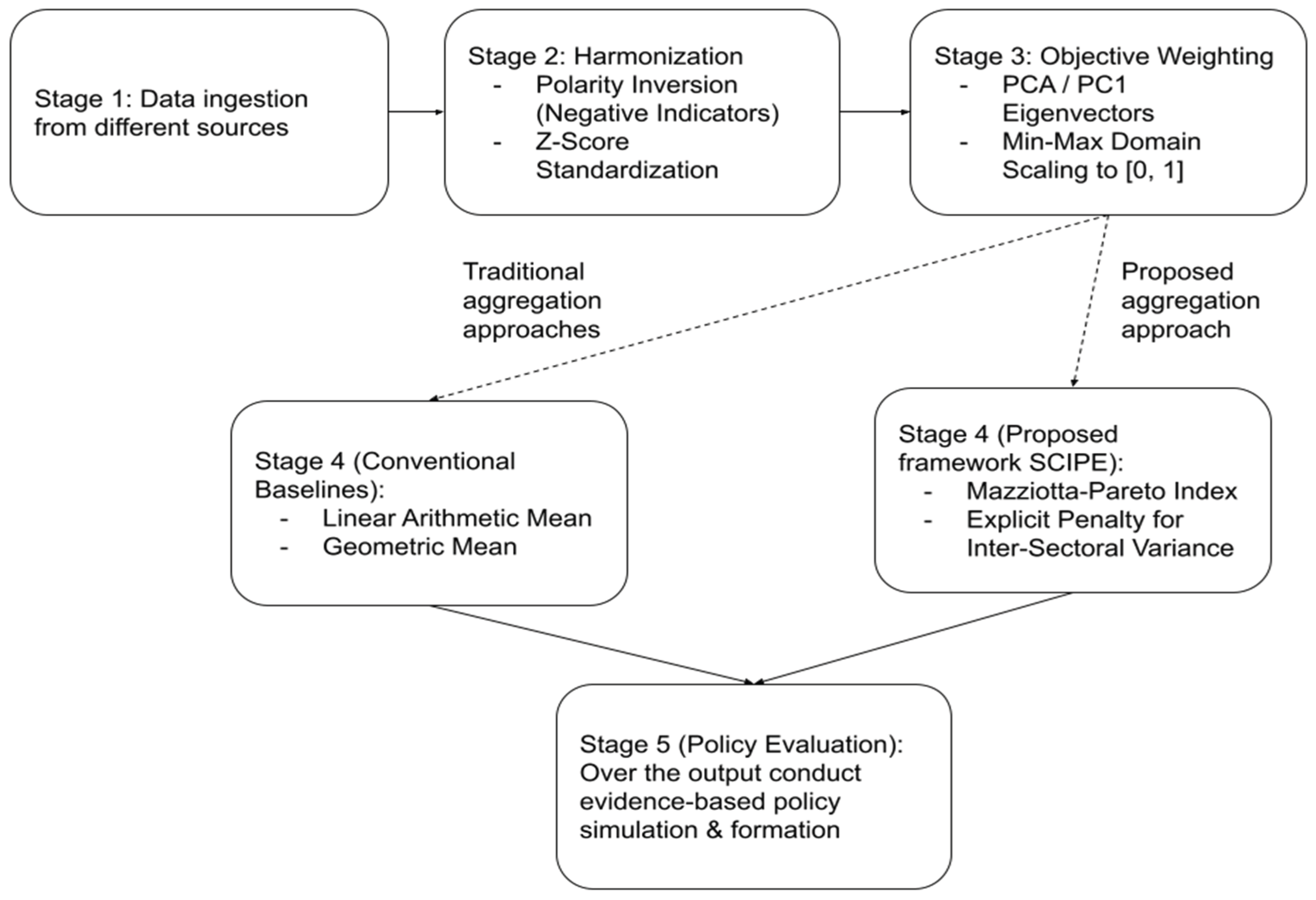
Figure 2.
Spatial distribution of SCIPE values across all 64 districts in Bangladesh. The map depicts the CI scores, utilizing a diverging and gradient color scale: green shades show higher QoL performance, while red shades indicate districts that receive lower aggregate scores or higher vulnerability. We also show the upper 5 and lower 5 districts as per the generated values.
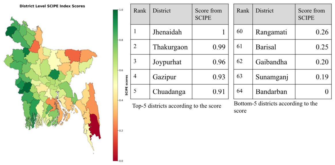
Figure 3.
Composite indicator distribution scores for districts.
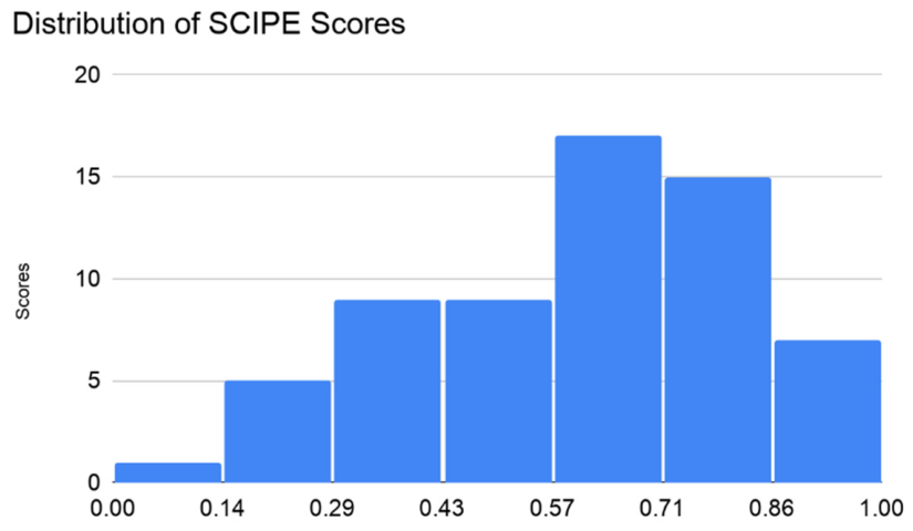
Figure 4.
Statistical Profile and Spatial Distribution of the Living Condition Scores.
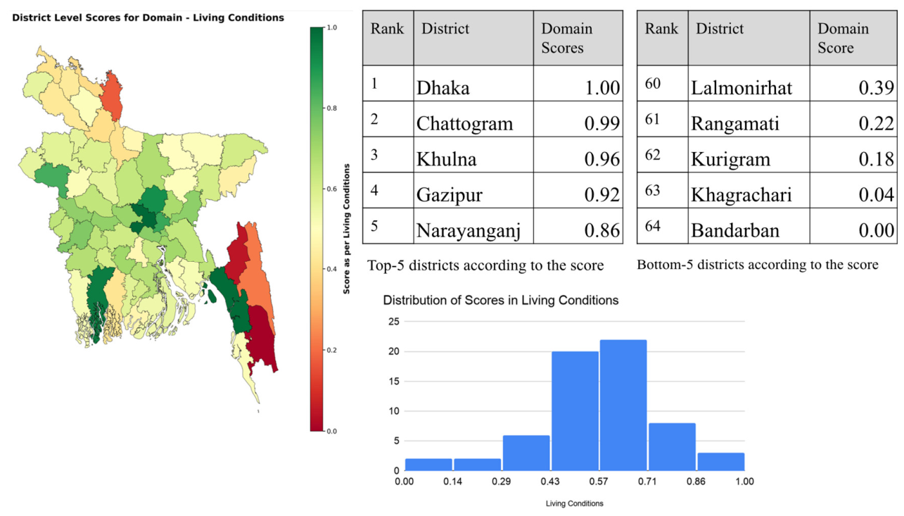
Figure 5.
Statistical Profile and Spatial Distribution of the Health Domain Scores.
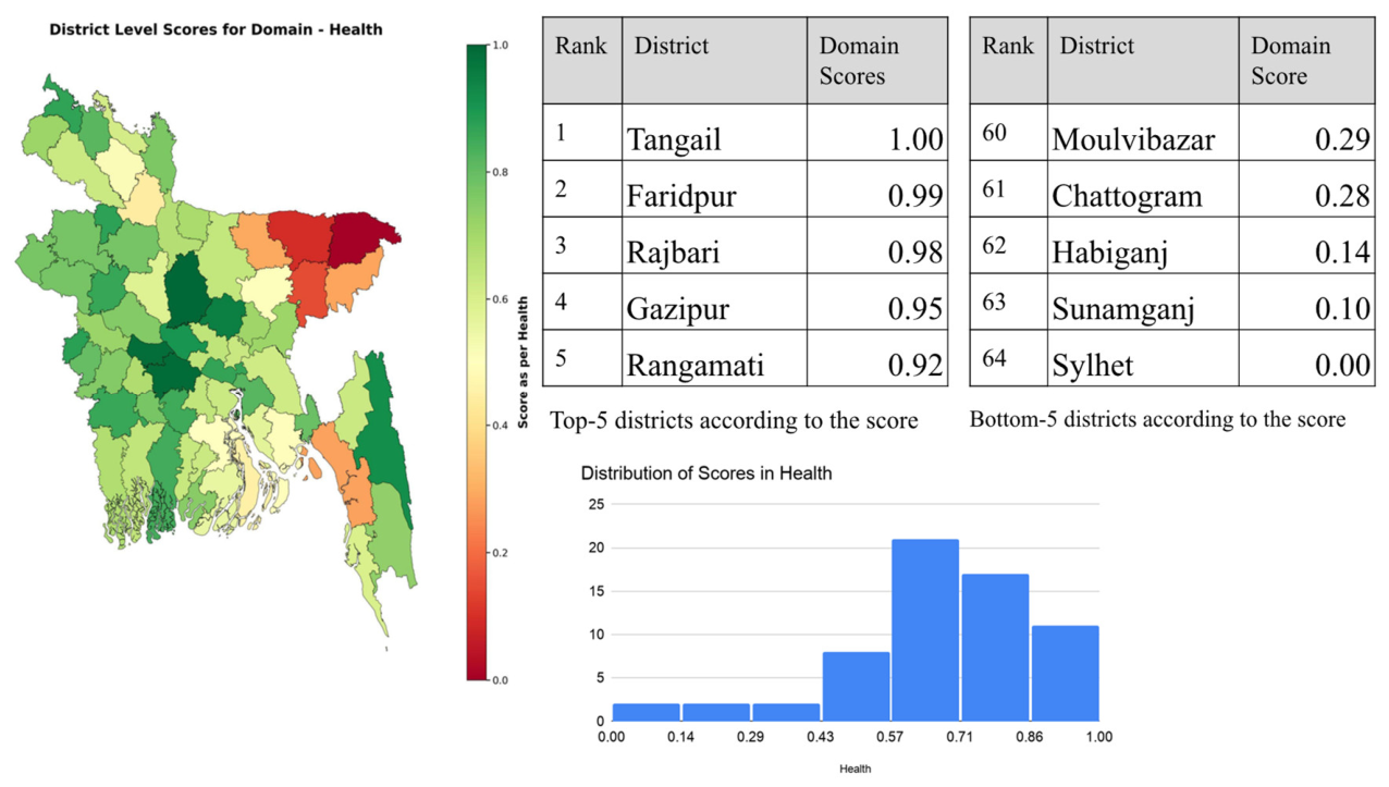
Figure 6.
Statistical Profile and Spatial Distribution of the Domain Scores in Education.
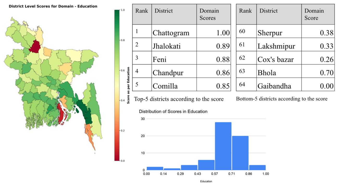
Figure 7.
Statistical Profile and Spatial Distribution of the Domain Scores from Infrastructure.
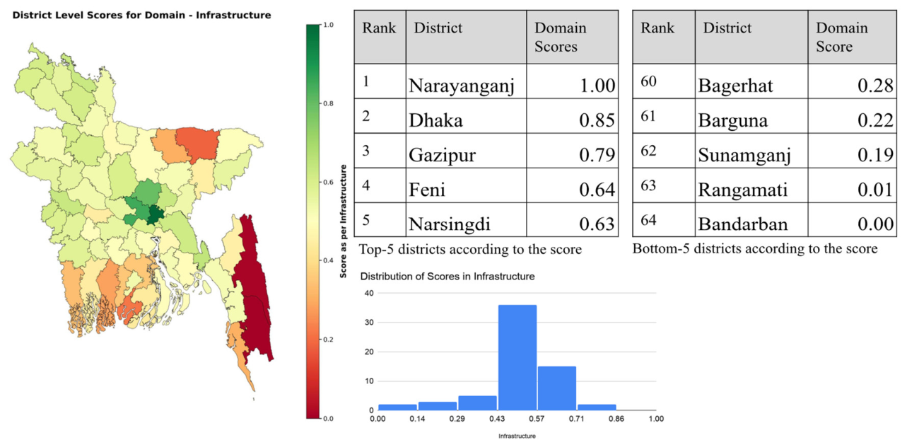
Figure 8.
Spatial Distribution and Statistical Profile of the Domain Scores associated with Environment.
Figure 8.
Spatial Distribution and Statistical Profile of the Domain Scores associated with Environment.
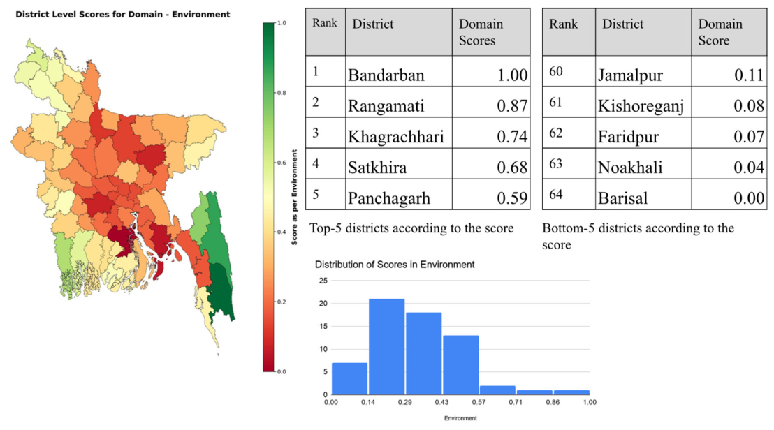
Figure 9.
Pearson Correlation Coefficient analysis within the domain variables and SCIPE index.
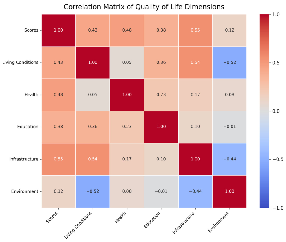
Figure 10.
Scatterplot of raw SCIPE scores against raw linear average scores. Districts (data points) are color-coded by the standard deviation of their individual domain scores.
Figure 10.
Scatterplot of raw SCIPE scores against raw linear average scores. Districts (data points) are color-coded by the standard deviation of their individual domain scores.
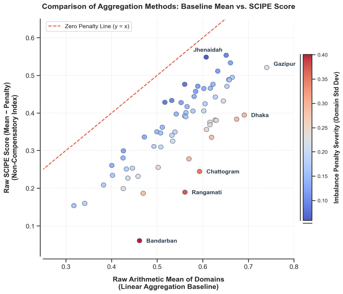

Table 1.
Mapping of SCIPE’s core domains, indicator directionality, and SDG alignment.
| Domain | Indicator | Data Source | Directionality | SDG Alignment |
|---|---|---|---|---|
| Living Conditions | Per Capita Income (BDT/Month) | Household Income and Expenditure Survey (2016) | Positive (+) | SDG 8 |
| Extreme Poverty Rate (%) | Household Income and Expenditure Survey (2016) | Negative (−) | SDG 1 | |
| Health | Under-5 Mortality Rate (%) | Demographic and Health Surveys (2014) | Negative (−) | SDG 3 |
| Stunting Rate (Nutrition) (%) | Demographic and Health Surveys (2014) | Negative (−) | SDG 2 | |
| Birth Registration (%) | Demographic and Health Surveys (2014) | Positive (+) | SDG 16 | |
| Education | Primary Completion Rate (%) | BANBEIS (2015) [2] | Positive (+) | SDG 4 |
| Infrastructure | Access to Electricity (%) | BDQOL Harmonized Census | Positive (+) | SDG 7 |
| Households Using Tubewells (%) | BDQOL Harmonized Census | Positive (+) | SDG 6 | |
| Households Using Sanitary Latrines (%) | BDQOL Harmonized Census | Positive (+) | SDG 6 | |
| Paved Roads (%) | Bangladesh Statistical Yearbook (2018) | Positive (+) | SDG 9 | |
| Nighttime Luminosity (NTL) | Wahed et al. (2020) [29] | Positive (+) | SDG 11 | |
| Environment | Air Quality (PM2.5) | Energy Policy Institute (2025) | Negative (−) | SDG 11 |
| Multihazard Risk Score | Islam (2017) [12] | Negative (−) | SDG 13 | |
| Reserve Forest Area (%) | Bangladesh Statistical Yearbook (2018) | Positive (+) | SDG 15 |
Table 2.
Domain-level PCA diagnostics, variance explained by PC1, eigenvector weights, and derived indicator weights.
Table 2.
Domain-level PCA diagnostics, variance explained by PC1, eigenvector weights, and derived indicator weights.
| Domain | Indicator | PC1 Variance (%) | Loading () | Normalized Weight () |
|---|---|---|---|---|
| Living Conditions | Access to Electricity | 35.09% | 0.6171 | 0.2949 |
| Living Conditions | Income and Employment | 0.4652 | 0.2223 | |
| Living Conditions | Poverty | 0.1844 | 0.0881 | |
| Living Conditions | Sanitation Facilities | 0.5309 | 0.2537 | |
| Living Conditions | Source of Drinking Water | 0.2949 | 0.1409 | |
| Health | Birth Registration | 45.22% | −0.4333 | 0.2546 |
| Health | Nutrition | 0.6968 | 0.4095 | |
| Health | Under 5 Mortality | 0.5716 | 0.3359 | |
| Education | Primary Education | 100.00% | 1 | 1 |
| Infrastructure | Paved Roads | 56.94% | 0.7071 | 0.5 |
| Infrastructure | NTL | 0.7071 | 0.5 | |
| Environment | Reserve forest area | 39.57% | 0.5788 | 0.3351 |
| Environment | Hazard Score | 0.6282 | 0.3638 | |
| Environment | Air Quality | 0.52 | 0.3011 |
Note: In our current setup, the Education domain comprises a single verified indicator at the district level, deterministically accounting for 100% of the domain score (w = 1.0).
Table 3.
Comparative scores and rank shifts between linear averaging and SCIPE.
| District | Raw Mean (Linear Baseline) | Linear Rank | Raw SCIPE Score | SCIPE Rank | Net Rank Shift | Raw Domain Disparity (Std Dev) |
|---|---|---|---|---|---|---|
| Thakurgaon | 0.608 | 21.0 | 0.548 | 2.0 | +19.0 | 0.059 |
| Jhenaidah | 0.651 | 9.0 | 0.553 | 1.0 | +8.0 | 0.098 |
| Gazipur | 0.740 | 1.0 | 0.521 | 4.0 | −3.0 | 0.219 |
| Dhaka | 0.691 | 2.0 | 0.395 | 28.0 | −26.0 | 0.296 |
| Narayanganj | 0.674 | 3.0 | 0.384 | 31.0 | −28.0 | 0.291 |
| Chattogram | 0.593 | 25.0 | 0.244 | 54.0 | −29.0 | 0.349 |
| Bandarban | 0.461 | 52.0 | 0.061 | 64.0 | −12.0 | 0.401 |
Table 4.
Aggregation Comparison of Top and Bottom District Outliers.
| District | Arithmetic Mean | Geometric Mean | Normalized SCIPE Score |
|---|---|---|---|
| Jhenaidah | 0.6513 | 0.6436 | 1.0000 |
| Thakurgaon | 0.6075 | 0.6047 | 0.9899 |
| Joypurhat | 0.6607 | 0.6492 | 0.9591 |
| Gaibandha | 0.3412 | 0.0500 | 0.2006 |
| Sunamganj | 0.3174 | 0.2673 | 0.1887 |
| Bandarban | 0.4613 | 0.0084 | 0.0000 |
Table 5.
Sensitivity analysis of district rank stability across alternative penalty scaling coefficients (R). Using (**), we highlight the performance of our baseline setup.
Table 5.
Sensitivity analysis of district rank stability across alternative penalty scaling coefficients (R). Using (**), we highlight the performance of our baseline setup.
| Penalty Coefficient (R) | Penalty Interpretation | Spearman Rank Correlation (ρ) | Statistical Significance (p-value) |
|---|---|---|---|
| R = 0.0 | Zero Penalty (Linear Arithmetic Mean) | 0.7682 | p = 1.28 × 10⁻¹³ |
| R = 0.5 | Moderate Variance Penalty | 0.9467 | p = 3.25 × 10⁻³² |
| R = 1.0 | Baseline SCIPE Specification** | 1 | — |
| R = 1.5 | Strong Variance Penalty | 0.9798 | p = 5.00 × 10−45 |
| R = 2.0 | Severe Variance Penalty | 0.9367 | p = 6.01 × 10⁻³⁰ |
Disclaimer/Publisher’s Note: The statements, opinions and data contained in all publications are solely those of the individual author(s) and contributor(s) and not of MDPI and/or the editor(s). MDPI and/or the editor(s) disclaim responsibility for any injury to people or property resulting from any ideas, methods, instructions or products referred to in the content. |
© 2026 by the authors. Licensee MDPI, Basel, Switzerland. This article is an open access article distributed under the terms and conditions of the Creative Commons Attribution (CC BY) license (http://creativecommons.org/licenses/by/4.0/).
Copyright: This open access article is published under a Creative Commons CC BY 4.0 license, which permit the free download, distribution, and reuse, provided that the author and preprint are cited in any reuse.