
Submitted:
15 September 2026
Posted:
16 September 2026
You are already at the latest version
Abstract
The receiver-side magnetic coupler in an electric vehicle wireless power transfer system must dissipate Litz-wire copper loss, ferrite-core loss, and eddy-current loss in the aluminum shield plate. After 60 min of continuous operation, the bare coil reached a hotspot temperature of 82.49 ℃. This left a 2.51 K margin below the 85 ℃ design criterion. We investigated passive thermal management using thermally conductive, electrically insulating silicone thermal interface materials (TIMs) at the coil–core and core–shield interfaces. Temperature-dependent loss models were coupled iteratively between ANSYS Maxwell and Icepak to assess TIM thermal conductivity, interface location, and coverage ratio. The two-way calculation converged after four coupling iterations, whereas a one-way calculation overestimated the total loss by approximately 5.7%. TIM-B had a measured thermal conductivity of 2.40 W m−1 K−1. At both interfaces and 100% coverage, it reduced the coil hotspot to 64.54 ℃, a decrease of 17.95 K. Either interface alone retained approximately 84% of the dual-interface temperature reduction. Among the tested coverage ratios, 110% produced the lowest hotspot temperature and the highest temperature uniformity index. These results provide quantitative guidance for selecting TIM locations and coverage in passively cooled wireless charging receivers.
Keywords:
wireless power transfer
; thermal interface material
; passive thermal management
; magnetothermal coupling
; finite-element analysis
; temperature uniformity
1. Introduction
Rapid growth in electric vehicle deployment has increased demand for charging systems that are convenient, weather-resistant, and suitable for automated operation [1]. Static wireless power transfer (WPT) eliminates exposed conductive connectors and is covered by SAE J2954 and the GB/T 38775 series [2,3]. Rounded-rectangular coils with series–series (SS) compensation are widely used because they distribute the air-gap magnetic field relatively evenly and fit vehicle packaging constraints [4]. However, higher charging power increases thermal loading in the receiver-side magnetic coupler. Temperature rise increases winding resistance and changes ferrite properties, which raises electromagnetic loss and reinforces further heating. Thermal management is therefore critical to the safe and efficient operation of high-power WPT systems.
Accurate thermal design begins with a representative description of the heat sources. Liang et al. [4] characterized the loss distribution in WPT magnetic couplers. Wang and Dorrell [5] and Lotfi and Lee [6] developed high-frequency loss models for Litz wire. Jiang et al. [7] incorporated temperature corrections to improve loss estimates at elevated temperatures. Many studies, however, emphasize total loss or a single hotspot temperature. Less attention has been given to spatially resolved heat sources and temperature feedback, although both are needed for interface-specific thermal design.
Thermal analysis of WPT systems has consequently progressed from one-way to two-way magneto-thermal coupling. Moghaddami and Sarwat [8] and Tiemann et al. [9] developed sequential coupling frameworks. Zimmer et al. [10] showed that one-way coupling can introduce substantial errors in thermal analyses of vehicle WPT modules. Ma et al. [11] refined the thermal boundary conditions used for magnetic-coupler simulations. These studies improved temperature prediction, but they did not establish quantitative rules for selecting individual TIM interfaces and coverage ratios.
Active cooling can reduce component temperatures, but pumps, channels, and seals add energy consumption, volume, and integration requirements [12,13]. Passive heat spreading with a TIM is simpler and avoids moving parts. Previous studies have shown that TIMs can improve heat transfer, but multiple interfaces are often treated as equivalent or covered uniformly [4,10]. The separate contributions of the coil–core and core–shield interfaces therefore remain unclear, as does the effect of extending the TIM beyond the ferrite area.
This study examines a WPT receiver with rounded-rectangular coils and SS compensation. We combine temperature-dependent models of Litz-wire copper loss, ferrite-core loss, and aluminum-shield eddy-current loss with iterative Maxwell–Icepak coupling. The model is then used to compare TIM thermal conductivity, interface location, and coverage ratio. A normalized temperature uniformity index (TUI) is evaluated alongside the hotspot temperature to distinguish peak suppression from spatial temperature uniformity.
2. Materials and Methods
2.1. System Configuration and Electrical Parameters
Table 1 lists the electrical parameters of the SS-compensated coils. The temperature dependence of the coil AC resistance was represented as
where R is the coil AC resistance, T is the coil temperature, and is the reference temperature. A higher temperature increases the AC resistance and copper loss, thereby introducing electrothermal feedback.

Table 1.
Electrical parameters of the rounded-rectangular SS-compensated coils.
| Parameter | Value | Parameter | Value |
|---|---|---|---|
| Primary self-inductance, | 202.74 H | Nominal resonant frequency, | 85 kHz |
| Secondary self-inductance, | 70.185 H | Ground clearance, | 230 mm |
| Primary AC resistance, | 0.11224 | Mutual inductance, M | 15.935 H |
| Secondary AC resistance, | 0.05776 |
The receiver-side coupler comprises a PEI coil tray, a Litz-wire coil, two TIM layers, MnZn PC95 ferrite tiles, a pure-aluminum shield plate, and a fiberglass enclosure. TIM-1 is located between the coil and ferrite core, whereas TIM-2 is located between the ferrite core and aluminum shield plate. Both TIMs provide heat conduction while maintaining electrical insulation. Figure 1 shows the principal receiver-side components and the two candidate TIM products.
2.2. Component Loss Models
The receiver-side magnetic coupler contains three principal heat sources: Litz-wire copper loss, ferrite-core loss, and eddy-current loss in the aluminum shield plate. Their physical mechanisms differ, but their temperature dependence couples them through the thermal field. Each loss distribution was calculated separately and mapped to the thermal model as a volumetric heat source.
2.2.1. High-Frequency Litz-Wire Copper Loss
At high frequency, copper loss is governed by skin and proximity effects. Litz wire suppresses the skin effect within each strand, but proximity fields still produce nonuniform AC loss. Maxwell was used to resolve the electromagnetic field and calculate the copper loss as
where is the DC resistance per unit length of one strand. Here, N is the number of turns, is the number of strands, and I is the RMS coil current. The field solution captures the local loss concentration caused by magnetic-field crowding around the rounded corners.
2.2.2. Ferrite-Core Loss
The improved generalized Steinmetz equation (iGSE) was used to describe core loss under nonsinusoidal excitation [14]. A temperature correction coefficient was applied before volume integration:
where is the volumetric ferrite loss and is the temperature correction coefficient for PC95 ferrite. The source model uses from 25 to °C and above °C.
Extrapolating the low-temperature expression above °C produces a correction-factor deviation that increases with temperature. The calculated deviation rises from 21.6% to 31.5% between 75 and °C. After volume integration across the internal temperature gradient, the ferrite-core loss may be underestimated by approximately 20–35%.
2.2.3. Eddy-Current Loss in the Aluminum Shield Plate
The alternating magnetic field induces macroscopic eddy currents in the aluminum shield plate. The characteristic penetration depth is
where f is the excitation frequency, is the permeability of free space, and is the electrical conductivity. For pure aluminum, S . At 85 kHz, Equation (4) gives a skin depth of approximately 0.28 mm, which is much smaller than the 8 mm plate thickness. The loss is therefore concentrated near the coil-facing surface. Maxwell calculated the spatial eddy-current loss, which was integrated as
This distribution was transferred to the thermal model as a spatially resolved heat source.
2.2.4. Loss Contributions at the Rated Condition
Table 2 summarizes the component losses at a 230 mm air gap and °C under resonant operation. The Litz-wire copper loss was 308.12 W and accounted for 59.41% of the total receiver-side loss. The coil was therefore the dominant heat source, making its heat-removal path the principal target of passive thermal management.
2.3. Thermal Model and Evaluation Metrics
2.3.1. Heat-Conduction Model
Steady-state heat conduction was governed by
where k is the position- and temperature-dependent thermal conductivity and q is the volumetric heat-generation rate. Their temperature dependence makes the model nonlinear and requires iteration with the electromagnetic solution.
The boundary conditions included natural convection, surface radiation, and interfacial conduction. Following the zonal treatment reported by Ma et al. [11], convection coefficients of 10, 7, and 5 W were applied to the top, side, and bottom surfaces, respectively. Surface radiation was included, and heat transfer across the solid interfaces was represented by the TIM thermal resistance.
2.3.2. TIM Interfacial Thermal Resistance
The nominal thermal resistance of a TIM layer was calculated as
where , , and A are the layer thickness, thermal conductivity, and contact area. At a coverage ratio , the uncovered area was occupied by air. The effective interface conductance therefore depended strongly on because air is much less conductive than either TIM.
For , the TIM extended beyond the ferrite-core outline. In this range, the additional material provided a lateral heat-spreading path rather than replacing an internal air gap. Parameterized geometries were used to evaluate both regimes.
2.3.3. Temperature Uniformity Index
The hotspot temperature determines the immediate insulation margin, but it does not describe the spatial temperature distribution. Two configurations can have similar hotspots but different average temperatures and local gradients. We therefore used the TUI as a complementary uniformity metric:
where and are the maximum and average coil temperatures. The subscript “ref” denotes the bare reference configuration. With this fixed normalization, a larger TUI indicates a smaller hotspot-to-average temperature difference. TUI does not measure the absolute hotspot temperature and must therefore be interpreted together with .
2.4. ANSYS Multiphysics Model
An iterative magneto-thermal model was implemented in ANSYS Electronics Desktop (AEDT). The Maxwell 3D Eddy Current solver calculated the electromagnetic field, and Icepak calculated the thermal field. Component losses were mapped from Maxwell to Icepak, and the updated temperatures were returned to Maxwell for the next coupling iteration. Figure 2 summarizes this workflow.
The Litz-wire coil was represented by an equivalent multi-turn racetrack geometry that retained the rounded-corner field concentration. The ferrite core and aluminum shield plate were modeled as homogeneous solids. Temperature-dependent electrical conductivity was assigned to copper and aluminum. The ferrite model included B–H and B–P data at 25, 60, 80, and °C. The simulated receiver self-inductance, mutual inductance, and coupling coefficient were H, H, and 0.134, respectively.
The Icepak model contained parameterized TIM-1 and TIM-2 solids. The outer boundary was defined as an Opening, with the convection coefficients and radiation conditions described above. A nonconforming mesh combined global coarse elements with local refinement at composite interfaces, air gaps, and other high-gradient regions. Figure 3 and Figure 4 show the Maxwell and Icepak meshes.
For each coupling iteration, Maxwell calculated the temperature-dependent electromagnetic losses and transferred them to Icepak as volumetric heat sources. Icepak then performed 20 internal thermal iterations before returning the component temperatures to Maxwell. Coupling continued until the maximum temperature change between successive exchanges was below °C and the total-loss change was below 1%.
3. Results and Discussion
Unless otherwise stated, the simulations used a 230 mm air gap, an ambient temperature of °C, and the reported condition after 60 min of continuous operation. The TUI values use the bare configuration as the fixed normalization reference.
3.1. Coupling Convergence and Loss Correction
Table 3 shows the loss evolution over four coupling iterations. The ferrite-core loss decreased from 239.80 W in the first iteration to 175.63 W in the fourth, a change of 26.7%. The total loss decreased from 548.02 to 518.65 W. Treating the first electromagnetic solution as a one-way result would therefore overestimate the converged total loss by approximately 5.7%.
The ferrite-core loss from the first iteration was approximately 36.6% higher than the converged value. This difference is large enough to affect a safety-margin assessment near the °C design criterion. Figure 5 shows the internal solver residuals and monitored temperatures. The energy residual reached approximately –, while the continuity residual remained near without divergence. The monitored temperatures approached stable values, and the total-loss change between iterations 3 and 4 was approximately 0.39%. Together, these indicators support convergence of the coupled solution.
3.2. Bare Reference Temperature Field
Table 4 summarizes the component temperatures of the bare reference. The coil, ferrite core, and aluminum shield plate showed progressively lower hotspot temperatures. This order is consistent with the dominant copper loss and the thermal resistance along the coil-to-shield heat path.
Turn-resolved temperatures are listed in Table 5. The highest local temperature occurred near the third turn in a rounded corner rather than at the geometric center. Field crowding in the corner increases skin and proximity effects, producing higher local AC loss than in the straight sections. The simulated temperature distribution in Figure 6 is consistent with this loss pattern.
The coil hotspot was only 2.51 K below the °C design criterion. As a first-order estimate, increasing the ambient temperature from 25 to °C while holding the temperature rise constant would increase the hotspot to approximately °C. This estimate does not include additional feedback from the temperature-dependent winding resistance. It therefore identifies a potential high-ambient-temperature risk, but it is not a substitute for a dedicated transient or high-ambient simulation.
3.3. Effect of TIM Thermal Conductivity
Table 6 lists the thermophysical properties used in the model. The room-temperature thermal conductivities of TIM-A and TIM-B were measured by laser flash analysis. TIM-B had a thermal conductivity 60% higher than TIM-A.
Under dual-interface, 100% coverage, both TIMs reduced the coil hotspot relative to the bare reference. TIM-A reduced the hotspot by 10.46 K, whereas TIM-B produced a 17.95 K reduction (Table 7). Figure 7 shows the corresponding component and coil temperature fields.
The temperature reduction did not scale linearly with TIM thermal conductivity. Heat from the coil passes through both interface resistances and the bulk ferrite resistance. Once the interface resistance becomes comparable to the ferrite resistance, further increases in TIM conductivity remove a smaller fraction of the total resistance. This series-resistance constraint explains the diminishing return. Both materials also reduced the hotspot-to-average temperature difference, with TIM-B producing the larger TUI.
3.4. Independent Contribution of Each TIM Interface
Table 8 compares TIM-B at the two interfaces. TIM-1 alone reduced the coil hotspot by 15.02 K, and TIM-2 alone produced a 15.28 K reduction. Each single-interface configuration therefore retained approximately 84% of the 17.95 K reduction achieved by the dual-interface configuration.
TIM-1 directly lowers the resistance between the dominant heat source and the ferrite core. TIM-2 instead lowers the core-to-shield resistance and reduces the ferrite temperature, increasing the driving temperature difference from the coil. These distinct heat-flow patterns produced similar hotspot reductions, as shown in Figure 8.
The reductions from the two single-interface cases are not additive. Lowering one interface resistance increases the relative importance of the other interface and the bulk component resistances. For hotspot control alone, one TIM layer retained more than 80% of the dual-interface reduction while using less material. The dual-interface configuration is preferable when temperatures across the ferrite and shield, as well as coil uniformity, are also design objectives.
3.5. Effect of TIM Coverage Ratio
The coverage ratio was defined relative to the ferrite-core area and varied from 60% to 120%. Ratios above 100% indicate that the TIM extended beyond the ferrite outline. Table 9 summarizes the resulting component hotspots and TUI values.
From 60% to 100% coverage, increasing the TIM area progressively replaced low-conductivity air gaps. The resulting reduction in interface resistance lowered the coil hotspot. Once coverage approached the full ferrite area, the bulk ferrite and other series resistances became more influential, reducing the incremental benefit.
Above 100% coverage, the additional TIM formed a lateral heat-spreading path outside the ferrite outline. The 110% case produced the lowest coil hotspot and the highest TUI among the tested ratios. Representative temperature fields are shown in Figure 9.
Figure 10 compares the hotspot and average coil temperatures. Both temperatures decreased overall as coverage increased. From 110% to 120%, the average temperature decreased further, but the hotspot increased by approximately 0.4 K. This hotspot change lies within the specified coupling-temperature tolerance and should not be interpreted as definitive evidence of a nonmonotonic physical response.
The TUI nevertheless decreased from 72.5% at 110% coverage to 67.0% at 120%. The additional peripheral TIM cooled the already cooler edge regions more effectively than the rounded-corner hotspot. This increased the hotspot-to-average temperature difference even as the average temperature continued to fall. A longer lateral conduction path may also limit the influence of the added peripheral area.
3.6. Temperature Uniformity and Design Selection
Table 10 compiles the hotspot, average temperature, and TUI for all investigated configurations. The TUI should be read together with the absolute hotspot temperature because Equation (8) measures only the normalized hotspot-to-average difference.
TIM-A reduced the hotspot below the °C design criterion at 100% coverage. TIM-B produced a larger reduction under the same geometry. When material use is constrained, either single-interface TIM-B configuration retains most of the dual-interface hotspot reduction. When hotspot temperature and spatial uniformity are both prioritized, the 110% dual-interface TIM-B case performed best among the discrete configurations tested here. This recommendation is specific to the present geometry, boundary conditions, and material properties.
4. Conclusions
This study combined temperature-dependent component-loss models with iterative Maxwell–Icepak coupling to evaluate passive thermal management in a WPT receiver. The two-way solution converged after four coupling iterations. A one-way treatment overestimated the converged total loss by approximately 5.7%, which could distort a temperature-margin assessment.
At dual-interface, 100% coverage, TIM-B reduced the coil hotspot from 82.49 to °C. Its measured thermal conductivity was 2.40 W . TIM-1 or TIM-2 alone retained approximately 84% of this temperature reduction. The nonadditive response reflects the changing balance among the two interface resistances and the bulk component resistances.
Increasing coverage from 60% to 110% reduced the coil hotspot by approximately 12 K and increased the TUI from 42.9% to 72.5%. The 110% case performed best among the tested ratios, while the 120% case produced no resolved hotspot improvement and a lower TUI. These values should not be generalized beyond the present simulated geometry and boundary conditions.
The results provide interface-selection and coverage guidance for passively cooled WPT receivers. Experimental validation remains necessary. Future work should compare the simulations with thermocouple and infrared measurements from a receiver prototype. It should also examine locally patterned TIM layouts and coordinated active–passive cooling strategies.
Author Contributions
Conceptualization, methodology, investigation, software, validation, formal analysis, data curation, writing, and visualization: to be completed by the authors. All authors have read and agreed to the published version of the manuscript.
Funding
This work was supported by the National Natural Science Foundation of China (Grant No. 52278424).
Institutional Review Board Statement
Not applicable.
Informed Consent Statement
Not applicable.
Data Availability Statement
The data presented in this study are available from the corresponding author upon reasonable request.
Conflicts of Interest
The authors declare no conflicts of interest.
Abbreviations
The following abbreviations are used in this manuscript:
| AEDT | ANSYS Electronics Desktop |
| iGSE | Improved generalized Steinmetz equation |
| SS | Series–series |
| TIM | Thermal interface material |
| TUI | Temperature uniformity index |
| WPT | Wireless power transfer |
References
- International Energy Agency. Global EV Outlook 2023, 2023. (accessed on 9 September 2026). [CrossRef]
- SAE International. SAE J2954: Wireless Power Transfer for Light-Duty Plug-In/Electric Vehicles and Alignment Methodology. 2020. [Google Scholar] [CrossRef]
- GB/T 38775.7-2021; Wireless Power Transfer System for Electric Vehicles—Part 7: Interoperability Requirements and Test Methods—Vehicle Side. National Technical Committee on Auto Standardization (SAC/TC 114), 2021.
- Liang, C.; Yang, G.; Yuan, F.; Huang, X.; Sun, Y.; Li, J.; Song, K. Modeling and Analysis of Thermal Characteristics of Magnetic Coupler for Wireless Electric Vehicle Charging System. IEEE Access 2020, 8, 173177–173185. [Google Scholar] [CrossRef]
- Wang, S.; Dorrell, D.G. Copper Loss Analysis of EV Charging Coupler. IEEE Trans. Magn. 2015, 51, 1–4. [Google Scholar] [CrossRef]
- Lotfi, A.W.; Lee, F.C. A High Frequency Model for Litz Wire for Switch-Mode Magnetics. In Proceedings of the 1993 IEEE Industry Applications Conference; IEEE, 1993; pp. 1169–1175. [Google Scholar] [CrossRef]
- Jiang, J.; Lan, Y.; Zhang, Z.; Zhou, X.; Song, K. Thermal Estimation and Thermal Design for Coupling Coils of 6.6 kW Wireless Electric Vehicle Charging System. Energies 2022, 15, 6797. [Google Scholar] [CrossRef]
- Moghaddami, M.; Sarwat, A. Time-Dependent Multi-Physics Analysis of Inductive Power Transfer Systems. In Proceedings of the 2018 IEEE Transportation Electrification Conference and Expo; IEEE, 2018; pp. 130–134. [Google Scholar] [CrossRef]
- Tiemann, M.; Saifo, M.; Clemens, M.; Schmuelling, B. Magnetic and Thermal Coupled Field Analysis of Wireless Charging Systems for Electric Vehicles. IEEE Trans. Magn. 2019, 55, 1–4. [Google Scholar] [CrossRef]
- Zimmer, S.; Helwig, M.; Winkler, A.; Modler, N. Comparison of One-Way and Two-Way Coupled Simulation for Thermal Investigation of Vehicular Wireless Power Transfer Modules. Eng 2023, 4, 816–828. [Google Scholar] [CrossRef]
- Ma, J.; Li, Z.; Liu, Y.; Ban, M.; Song, W. Thermal Analysis and Optimization of the Magnetic Coupler for Wireless Charging System. IEEE Trans. Power Electron. 2023, 38, 16269–16280. [Google Scholar] [CrossRef]
- Zhang, Z. Loss Calculation and Thermal Management of Magnetic Couplers for Wireless Charging Systems. PhD thesis, Harbin Institute of Technology, Harbin, China, 2022. [Google Scholar]
- Ye, L.; Li, X.; Li, D. Magnetothermal Analysis and Experiment of a Water-Cooled Eddy-Current Retarder Coil. J. Beijing Univ. Technol. 2022, 48, 1122–1131. (In Chinese) [Google Scholar]
- Venkatachalam, K.; Sullivan, C.R.; Abdallah, T.; Tacca, H. Accurate Prediction of Ferrite Core Loss with Nonsinusoidal Waveforms Using Only Steinmetz Parameters. In Proceedings of the IEEE Workshop on Computers in Power Electronics; IEEE, 2002; pp. 36–41. [Google Scholar] [CrossRef]
Figure 1.
Photographs of the principal receiver-side components and TIM samples. Clockwise from the upper left: rounded-rectangular receiver coil; TIM-A and TIM-B sheets; MnZn PC95 ferrite-core tile assembly; and aluminum shield plate. The dimensions shown in the photographs are the nominal model dimensions.
Figure 1.
Photographs of the principal receiver-side components and TIM samples. Clockwise from the upper left: rounded-rectangular receiver coil; TIM-A and TIM-B sheets; MnZn PC95 ferrite-core tile assembly; and aluminum shield plate. The dimensions shown in the photographs are the nominal model dimensions.
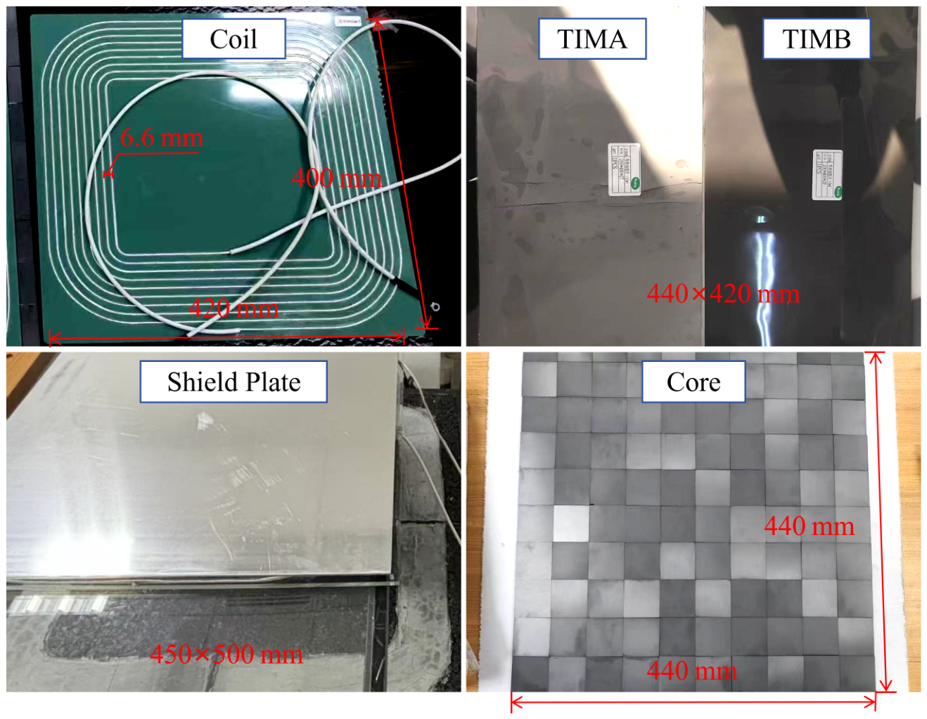
Figure 2.
Iterative Maxwell–Icepak simulation workflow used for two-way magneto-thermal coupling.
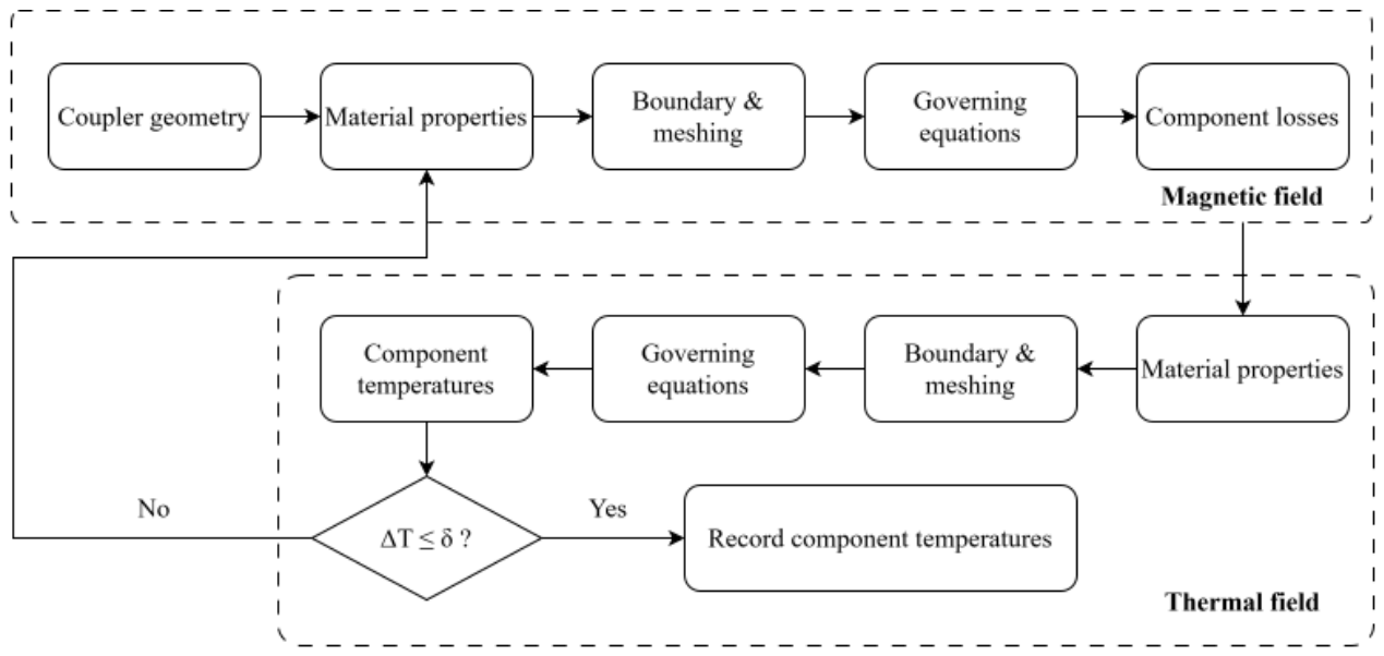
Figure 3.
Maxwell mesh for the receiver-side model: (a) aluminum shield plate; (b) ferrite core; (c) receiver coil; and (d) local coil region.
Figure 3.
Maxwell mesh for the receiver-side model: (a) aluminum shield plate; (b) ferrite core; (c) receiver coil; and (d) local coil region.
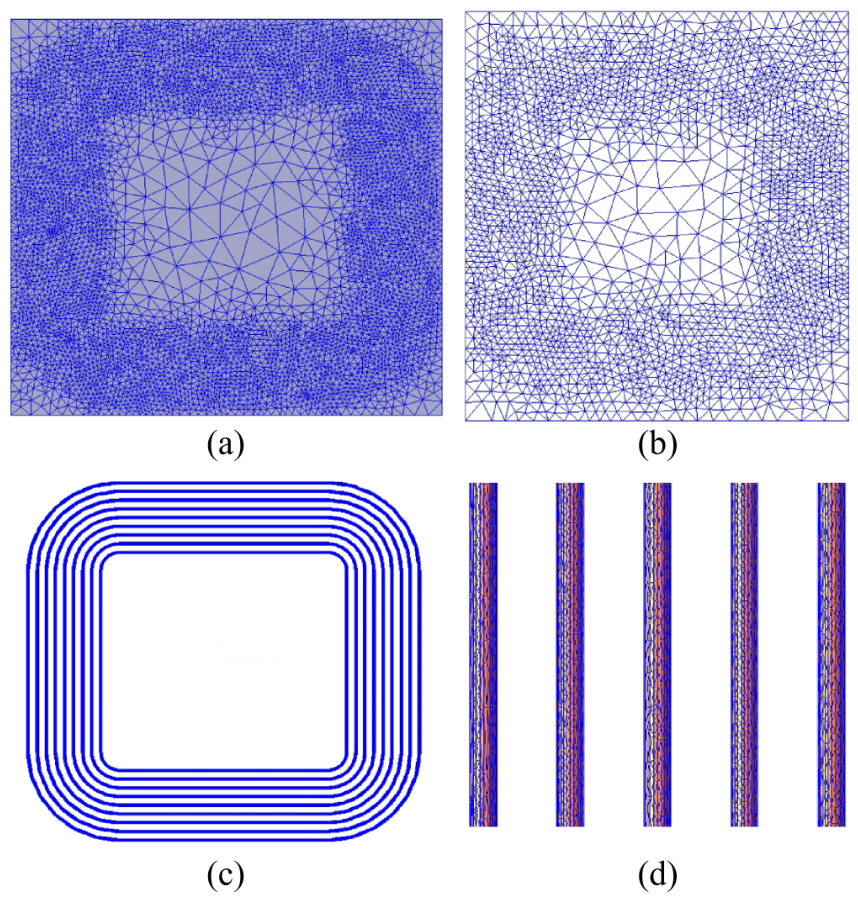
Figure 4.
Icepak mesh for the receiver-side model: (a) aluminum shield plate; (b) ferrite core; (c) receiver coil; and (d) local coil region.
Figure 4.
Icepak mesh for the receiver-side model: (a) aluminum shield plate; (b) ferrite core; (c) receiver coil; and (d) local coil region.
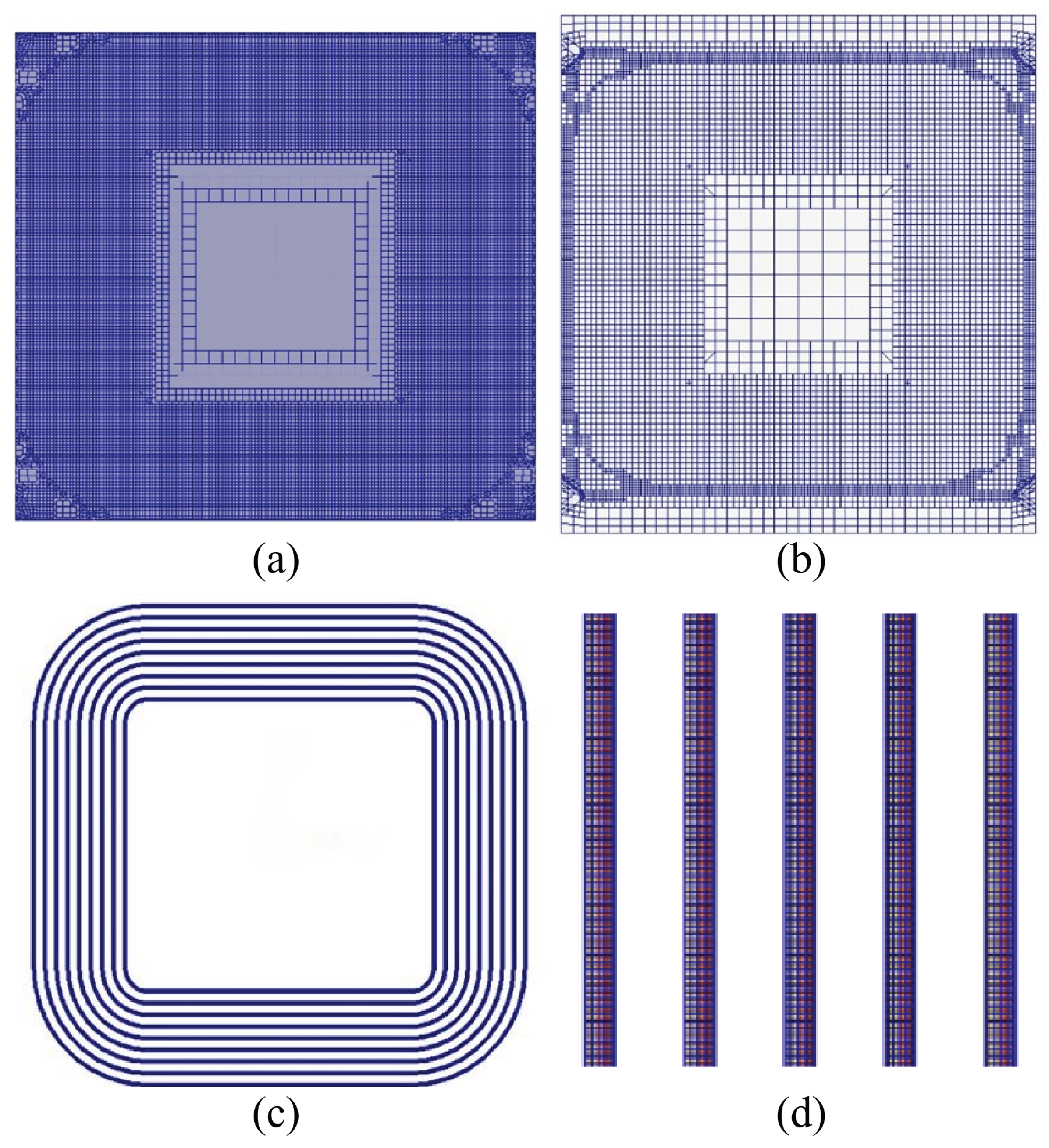
Figure 5.
Convergence of the coupled simulation: (a) residual histories of the continuity and energy equations; and (b) temperature histories at the monitored component locations.
Figure 5.
Convergence of the coupled simulation: (a) residual histories of the continuity and energy equations; and (b) temperature histories at the monitored component locations.
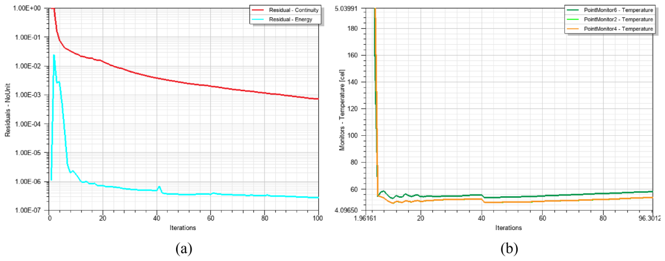
Figure 6.
Temperature field of the bare reference configuration: (a) complete receiver-side model; and (b) receiver coil.
Figure 6.
Temperature field of the bare reference configuration: (a) complete receiver-side model; and (b) receiver coil.
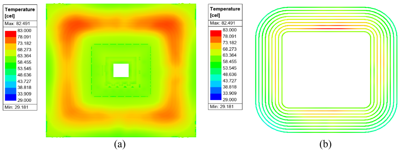
Figure 7.
Temperature fields under dual-interface, 100% coverage: (a) complete model with TIM-A; (b) complete model with TIM-B; (c) coil with TIM-A; and (d) coil with TIM-B.
Figure 7.
Temperature fields under dual-interface, 100% coverage: (a) complete model with TIM-A; (b) complete model with TIM-B; (c) coil with TIM-A; and (d) coil with TIM-B.
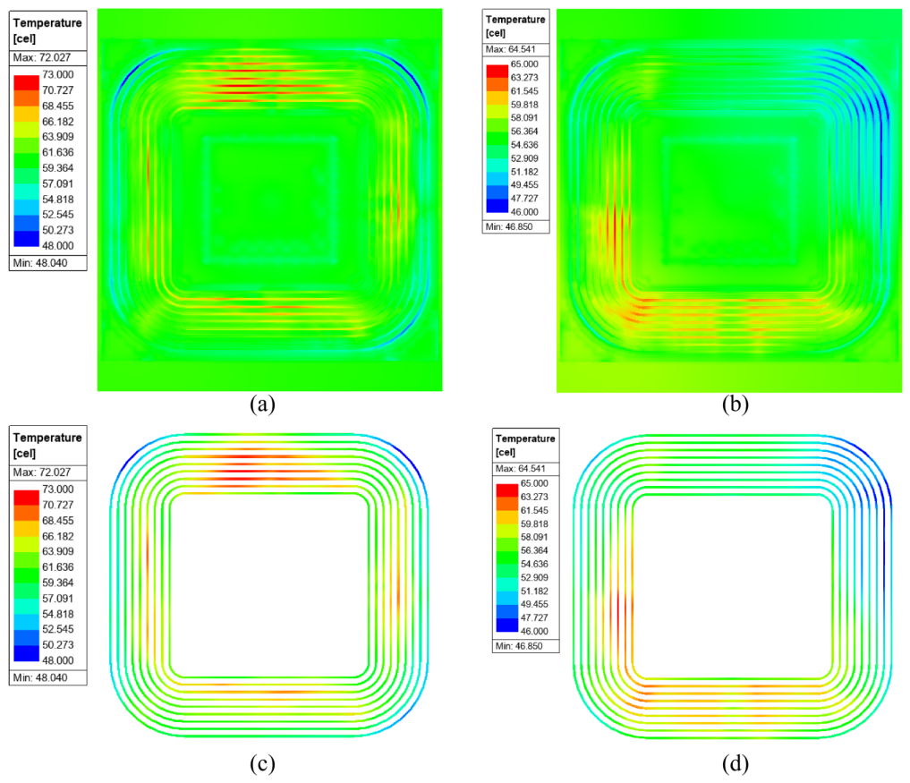
Figure 8.
Temperature fields for the two single-interface configurations: (a) TIM-1 only; and (b) TIM-2 only.
Figure 8.
Temperature fields for the two single-interface configurations: (a) TIM-1 only; and (b) TIM-2 only.
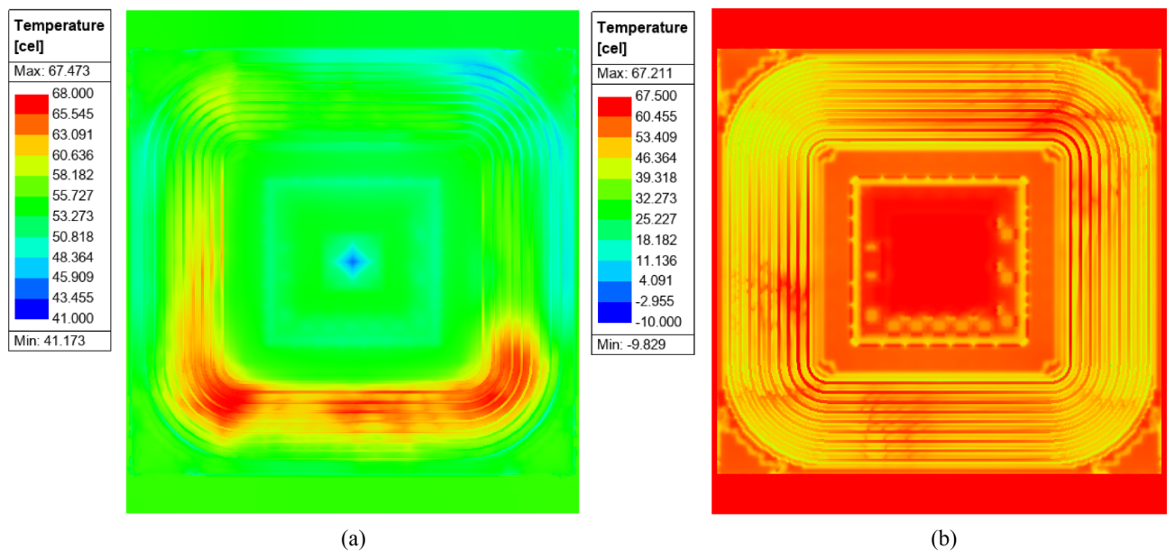
Figure 9.
Temperature fields for selected TIM-B coverage ratios: (a) 60%; (b) 80%; (c) 110%; and (d) 120%. Subscript 1 denotes the complete receiver-side model, and subscript 2 denotes the receiver coil.
Figure 9.
Temperature fields for selected TIM-B coverage ratios: (a) 60%; (b) 80%; (c) 110%; and (d) 120%. Subscript 1 denotes the complete receiver-side model, and subscript 2 denotes the receiver coil.
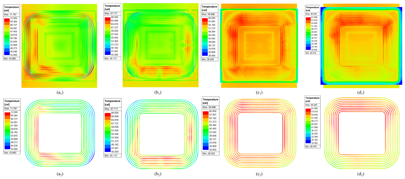
Figure 10.
Coil hotspot and average temperatures as functions of the TIM-B coverage ratio in the dual-interface configuration.
Figure 10.
Coil hotspot and average temperatures as functions of the TIM-B coverage ratio in the dual-interface configuration.
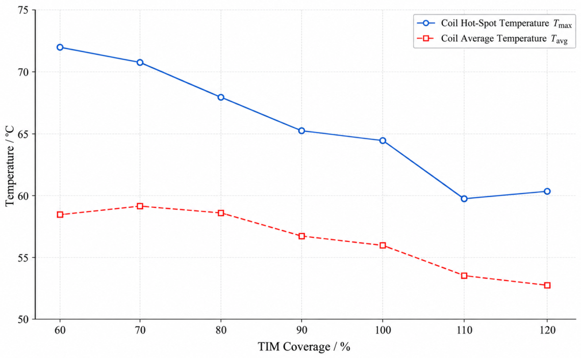
Table 2.
Electromagnetic loss distribution at the rated operating condition.
| Loss component | Loss (W) | Fraction (%) |
|---|---|---|
| Litz-wire copper loss, | 308.12 | 59.41 |
| Ferrite-core loss, | 175.63 | 33.86 |
| Aluminum-shield eddy-current loss, | 34.90 | 6.73 |
| Total receiver-side loss, | 518.65 | 100.00 |
Table 3.
Evolution of component losses during two-way magneto-thermal coupling.
| Loss component (W) | Iteration 1 | Iteration 2 | Iteration 3 | Iteration 4 |
|---|---|---|---|---|
| Litz-wire coil | 278.01 | 306.25 | 306.94 | 308.12 |
| Ferrite core | 239.80 | 175.65 | 179.13 | 175.63 |
| Aluminum shield plate | 30.21 | 34.86 | 34.62 | 34.90 |
| Total | 548.02 | 516.76 | 520.69 | 518.65 |
Table 4.
Thermal characteristics of the bare reference configuration.
| Component | Hotspot temperature (°C) | Temperature rise (K) |
|---|---|---|
| Litz-wire coil | 82.49 | 57.49 |
| Ferrite core | 74.92 | 49.92 |
| Aluminum shield plate | 63.62 | 38.62 |
Table 5.
Turn-by-turn average temperature of the bare receiver coil. Turns are numbered from the inner to the outer winding.
Table 5.
Turn-by-turn average temperature of the bare receiver coil. Turns are numbered from the inner to the outer winding.
| Turn | 1 | 2 | 3 | 4 | 5 | 6 | 7 | 8 | 9 |
|---|---|---|---|---|---|---|---|---|---|
| Average temperature (°C) | 61.74 | 67.03 | 67.85 | 64.92 | 61.61 | 59.47 | 56.77 | 53.23 | 51.58 |
Table 6.
Thermophysical properties used in the thermal model.
| Component | Material | k (W ) | (kg ) | (J ) | |
|---|---|---|---|---|---|
| Litz-wire coil | Homogenized copper | 385.00 | 4967 | 385 | 0.80 |
| Ferrite core | PC95 MnZn ferrite | 5.00 | 4900 | 750 | 0.74 |
| Aluminum shield plate | Pure aluminum | 237.50 | 2700 | 900 | 0.50 |
| TIM-A | Insulating silicone | 1.50 | 2843 | 872 | – |
| TIM-B | Insulating silicone | 2.40 | 3577 | 800 | – |
Table 7.
Effect of TIM thermal conductivity under dual-interface, 100% coverage.
| Configuration | Coil hotspot | Core hotspot | Shield hotspot | Coil reduction | TUI |
|---|---|---|---|---|---|
| (°C) | (°C) | (°C) | (K) | (%) | |
| Bare reference | 82.49 | 74.92 | 63.62 | – | 0.0 |
| TIM-A, 1.50 W | 72.03 | 64.72 | 61.45 | 10.46 | 57.2 |
| TIM-B, 2.40 W | 64.54 | 59.98 | 57.98 | 17.95 | 62.3 |
Table 8.
Effect of TIM-B interface location under 100% coverage.
| TIM configuration | Coil hotspot (°C) | Reduction from bare reference (K) |
|---|---|---|
| No TIM | 82.49 | – |
| TIM-1 only | 67.47 | 15.02 |
| TIM-2 only | 67.21 | 15.28 |
| TIM-1 and TIM-2 | 64.54 | 17.95 |
Table 9.
Effect of TIM-B coverage ratio in the dual-interface configuration.
| Coverage | Coil hotspot | Core hotspot | Shield hotspot | Difference from 100% | TUI |
|---|---|---|---|---|---|
| (%) | (°C) | (°C) | (°C) | (K) | (%) |
| 60 | 71.79 | 68.26 | 65.06 | +7.25 | 42.9 |
| 70 | 70.59 | 65.51 | 63.48 | +6.05 | 50.3 |
| 80 | 67.72 | 63.16 | 61.45 | +3.18 | 60.7 |
| 90 | 65.27 | 60.45 | 59.20 | +0.73 | 62.8 |
| 100 | 64.54 | 59.98 | 57.98 | 0.00 | 62.3 |
| 110 | 59.90 | 56.06 | 53.88 | -4.64 | 72.5 |
| 120 | 60.28 | 55.92 | 53.50 | -4.26 | 67.0 |
Table 10.
Temperature uniformity index for the investigated TIM configurations.
| Configuration | (°C) | (°C) | (K) | TUI (%) |
|---|---|---|---|---|
| Bare reference | 82.491 | 59.721 | 22.770 | 0.0 |
| TIM-A, dual interface, 100% | 72.027 | 62.277 | 9.750 | 57.2 |
| TIM-B, TIM-1 only, 100% | 67.473 | 56.658 | 10.815 | 52.5 |
| TIM-B, TIM-2 only, 100% | 67.211 | 54.035 | 13.176 | 42.1 |
| TIM-B, dual interface, 60% | 71.787 | 58.793 | 12.994 | 42.9 |
| TIM-B, dual interface, 70% | 70.593 | 59.283 | 11.310 | 50.3 |
| TIM-B, dual interface, 80% | 67.717 | 58.765 | 8.952 | 60.7 |
| TIM-B, dual interface, 90% | 65.270 | 56.793 | 8.477 | 62.8 |
| TIM-B, dual interface, 100% | 64.541 | 55.947 | 8.594 | 62.3 |
| TIM-B, dual interface, 110% | 59.898 | 53.644 | 6.254 | 72.5 |
| TIM-B, dual interface, 120% | 60.282 | 52.776 | 7.506 | 67.0 |
Disclaimer/Publisher’s Note: The statements, opinions and data contained in all publications are solely those of the individual author(s) and contributor(s) and not of MDPI and/or the editor(s). MDPI and/or the editor(s) disclaim responsibility for any injury to people or property resulting from any ideas, methods, instructions or products referred to in the content. |
© 2026 by the authors. Licensee MDPI, Basel, Switzerland. This article is an open access article distributed under the terms and conditions of the Creative Commons Attribution (CC BY) license (http://creativecommons.org/licenses/by/4.0/).
Copyright: This open access article is published under a Creative Commons CC BY 4.0 license, which permit the free download, distribution, and reuse, provided that the author and preprint are cited in any reuse.