

Submitted:
16 September 2026
Posted:
16 September 2026
You are already at the latest version
Abstract
A solid oxide electrolyser coupled to photovoltaic (PV) power must be operated through production, hot standby and night states rather than at a single design point. This work presents a Modelica dynamic model of the complete balance of plant (BoP) of the 25 kW PROMETEO pilot electrolyser, in which ten control loops and a supervisory state machine are driven by the available PV power through a capacity-factor logic with hysteresis. The stack model is validated against 5 kW polarisation data with a relative error below 3%. The constant-voltage, temperature-tracking strategy of the PROMETEO test campaign is simulated over a clear-sky day and an intermittent-cloud day. With a stack thermal capacity of 25 kJ/K and a direct stack heater, the stack is thermally neutral at 1.32 V/cell: the electrochemical heat balances the insulation losses, the sweep-air loop rests at the blower minimum and the current is tracked through the inlet temperatures alone, giving 14.1 kg of hydrogen at 44 kWh/kg over two days. A voltage sensitivity shows that output and specific consumption are flat within the feasible window, which is narrow: below 1.30 V/cell the stack exceeds its 780 °C limit, above 1.34 V/cell the current becomes steam-limited and the stack overheats, so that a current or steam protection is required. The strategy is robust to an eightfold change of the stack thermal capacity. The sweep-air loop must be disabled outside production and coordinated with the temperature references, otherwise blower and heaters saturate and the stack cools.
Keywords:
solid oxide electrolysis
; balance of plant
; dynamic modelling
; Modelica
; control strategy
; photovoltaic-driven hydrogen production
1. Introduction
Intermittent renewable energy sources (RES) require complementary storage to keep the grid stable [1,2,3,4]. Hydrogen is an attractive carrier because it is carbon-free [5] and efficiently converted in electrochemical devices [6,7]; it stores renewable electricity in chemical form [8] and supports the decarbonisation of transport, microgrids and industry [9,10,11,12]. Water electrolysis is the dominant route to high-purity hydrogen [13], with a share projected to rise from 4% [5] to 51% of hydrogen production by 2050 [14]. Among the technologies, solid oxide electrolysis cells (SOEC) benefit from a high operating temperature (680–1000 °C), which improves kinetics, and from waste-heat integration, which can reduce the electricity consumption per kilogram of hydrogen by up to 30% [15]; in SOEC balance-of-plant (BoP) configurations the sweep-air flow governs both the stack temperature and the pressure losses of the heat-exchanger network [16].
Because of the fluctuating RES input the plant undergoes frequent transients between full and partial load and between production and standby, so that dynamic models of heat transfer, fluid flow and electrochemistry are needed to design the control strategy. Yin et al. [17] analysed the response of an SOEC system to inlet temperature and flow variations; Saeedmanesh et al. [18] coupled an SOEC with PV input under feedback control; Botta et al. [20] developed PI control for a reversible system; Zhang et al. [21] reduced consumption through thermal control. These works treat the production state and do not address standby and idle states or the supervisory logic that sequences them. A complementary steady-state and annual analysis of the PROMETEO concept, scaled to 100 kW, has been reported by Barreto et al. [24], treating each mode at steady state; the control options for the pilot were defined by Crespi et al. [33] from a 5 kW test campaign.
This work presents a dynamic model of the complete 25 kW PROMETEO system, stack and BoP, developed in the Modelica language [22] with Modelon Impact 2.1.25 and the Modelon, Fuel Cell and Thermal Power libraries [23], chosen for the equation-based, acausal handling of the bidirectional couplings between stack and BoP. The second control option of [33], constant voltage with steam fixed per state and load tracked through the stack temperature, is implemented and verified over a clear-sky day and a synthetic intermittent-cloud day. The contribution is threefold: the dynamics of the complete BoP are resolved across production, hot standby and night mode under a PV-driven supervisory logic with hysteresis; the feasible window of the constant-voltage strategy is identified through sensitivity analyses on the stack voltage and on the stack thermal capacity; and a control-structure requirement invisible to steady-state or production-only analyses is exposed, namely that the sweep-air loop must be disabled outside production and coordinated with the temperature references. The aim is to identify inconsistencies in process and control design ahead of commissioning.
2. Methodology
2.1. The PROMETEO System and its Operating States
The PROMETEO project targeted a 25 kW pilot plant at an existing PV facility in Cuenca, Spain, integrating an SOEC BoP with PV electricity and solar thermal heat, so that hydrogen production is decoupled from heat availability. The BoP comprises four functional zones: steam generation from the solar heat-transfer-fluid (HTF) loop, mixing and preheating of fuel and air by waste-heat recovery, hydrogen production in the stack, and hydrogen post-treatment, recirculation and storage. Three supervisory states are defined (Table 1). In Production operating mode, the stack is connected at constant voltage and the load follows the PV power continuously between 150 and 256 A; the steam flow is set at one of two levels according to the current target, 1.50 g/s below 185 A and 2.56 g/s above, sized for a steam utilisation of 75% at 150 and 256 A (54–92% in between). In Hot Standby (HSB) the stack is disconnected while steam flow, hydrogen fraction and stack temperature are maintained; in Night Mode (NM) steam is stopped and a forming-gas mixture (N2/H2 80/20 vol.) is recirculated to protect the electrodes.
2.2. Balance-of-Plant Model
Fluid properties are handled through Modelon media models and NASA Glenn coefficients [25]: Water IF97 [26], Therminol 66 [27], the seven-species ideal-gas mixture NasaReformateLong, its condensing extension and NasaMoistAir [21], with medium converters at the zone boundaries [28]. Figure 1 shows the process flow diagram. Steam is raised in the generator E102 from the solar HTF, with demineralised water at 3 bar preheated in the economiser E101; the steam flow is modulated by a lamination valve and the drum pressure by the HTF flow. Steam superheating and air preheating take place in the plate heat exchangers (HEX) E103 and E104 by recovery from the stack off-gases. Downstream of E103 the steam is mixed with a hydrogen-rich stream recirculated from the cold BoP, where it has been cooled, dewatered in the water knock-out (WKO) and recompressed, to give 10% hydrogen in the cathode feed. Dry air is the anode sweep gas, and electric heaters upstream of both inlets bring the streams to the stack inlet temperature.
The stack and the heat exchangers are one-dimensional models discretised along the flow (N = 5 for the stack, N = 3 for the gas/gas HEX); the steam drum, the condensing separator and the cold-side gas volumes are lumped dynamic volumes; valves, blowers and sources are algebraic. All components except the stack are adiabatic; the stack exchanges heat with the 25 °C environment through a multilayer insulation model. The component list, modelling approach and parametrisation are given in Appendix A (Table A1) and Appendix F (Table F1); the layout in Modelon Impact is shown in Figure 2. The stack voltage is imposed by an ideal source. The solar HTF loop is a constant-temperature source at 200 °C, consistent with the molten-salt thermal store interposed between the solar field and E102; with steam raised at 3 bar (133.5 °C) and an HTF flow of 0.10 kg/s at full load, one fifth of the pump range, a 30 K drop of the HTF temperature would be absorbed by a 60% increase of the flow. The stack disconnection is an instantaneous Boolean event. The sweep-air blower is an ideal mass-flow source bounded at 0.002–0.040 kg/s, its consumption estimated from the network pressure drop with blower and motor efficiencies of 0.55 and 0.90, Eq. (15). The stack has a lumped thermal capacity of 25 kJ/K, i.e., 50 kg of cell and interconnect material at 500 J/(kg K), distributed over the five segments, while the HEX walls are massless, so that the stack is the only thermal inertia of the hot zone; a direct electric heater on the stack body, as installed on the pilot, is included with its own loop (Section 2.5).
2.3. Stack Model
The elementary cell model of the Fuel Cell Library (Figure 3) lumps the n_cell = 80 series-connected cells and is discretised in N = 5 segments along the flow. Electrically, each segment is a branch with a voltage source and the resistances of the ohmic loss and of the concentration overvoltage; the N branches are in parallel between the stack terminals, so that all segments share the terminal voltage while the current divides according to local temperature and composition. The open-circuit voltage of a segment is the Nernst voltage of the water-splitting reaction [20]:
where F is the Faraday constant, p0 = 1 atm and ΔG_r(T_cell) is the Gibbs free energy of reaction (R1), evaluated from the formation properties of the species [25] (about 188 kJ/mol at 800 °C, i.e., 0.98 V); the partial pressures are those of the segment (Appendix E). Under load the ohmic and concentration overvoltages of a single cell are
where j is the local current density, ASR the area-specific resistance, α the charge-transfer coefficient and U_steam the local steam utilisation. The terminal voltage and the stack current follow from the series connection of the cells within a segment and the parallel connection of the branches:
with I_j the current of segment j and A_cell/N its area; Eq. (5) defines the internal resistance R_int = n_cell N ASR/A_cell identified from the polarisation curves (Section 2.4). The ASR follows an Arrhenius law with respect to T0 = 1073 K [17]:
The steam utilisation is the ratio between the water consumed, from Faraday’s law for the n_cell cells, and the steam fed to the stack,
where MM_H2O is the molar mass of water and ṁ_steam the inlet steam flow; the same expression per segment gives the local utilisation of Eq. (3). The species exchanged with the channels follow from Faraday’s law in each segment,
with ν = −1 for H2O and +1 for H2 at the cathode and ν = 1/2 for O2 at the anode. The library uses the fuel-cell sign convention, so that the stack current I_SOE is negative in electrolysis and its absolute value is used in the balances, and the hydrogen production is
The electrical power of a segment is P_j = V_stack I_j; the cell energy balance and the enthalpy flows exchanged with the channels are given in Appendix E.
2.4. Stack Calibration, Validation and Scale-Up
The stack parameters ASR0, E_a and α were calibrated on the experimental data of Figure 4 and the calibrated model was validated on the polarisation curves of Figure 5. Figure 4 shows the voltage versus steam utilisation measured on the 5 kW test bench of the FBK laboratories reported by Crespi et al. [33]: a modified SolydEra G8-80 stack of 70 cells of 80 cm2, at ambient pressure between 680 and 780 °C, with steam flow varied stepwise from 360 to 1900 g/h, inlet temperatures from 670 to 760 °C and 10% hydrogen in the feed; the voltage was held at the thermoneutral value and the current was the measured output.
To calibrate ASR0 and E_a, data at open-circuit voltages of 1.282–1.284 V and flow rates above 1200 g/h were selected, so that ohmic losses dominate, and ASR was regressed linearly against (1/T − 1/T0) [34], giving ASR0 = 0.330 Ω cm2 at 800 °C and E_a = 80.7 kJ/mol. With these values and α = 0.5, Figure 5a compares simulated and experimental polarisation curves for five experiments spanning the steam-flow range and Figure 5b the relative error,
Figure 5.
a. Validation of the polarisation curves for the five selected experiments (simulation dotted, experiments solid).
Figure 5.
a. Validation of the polarisation curves for the five selected experiments (simulation dotted, experiments solid).
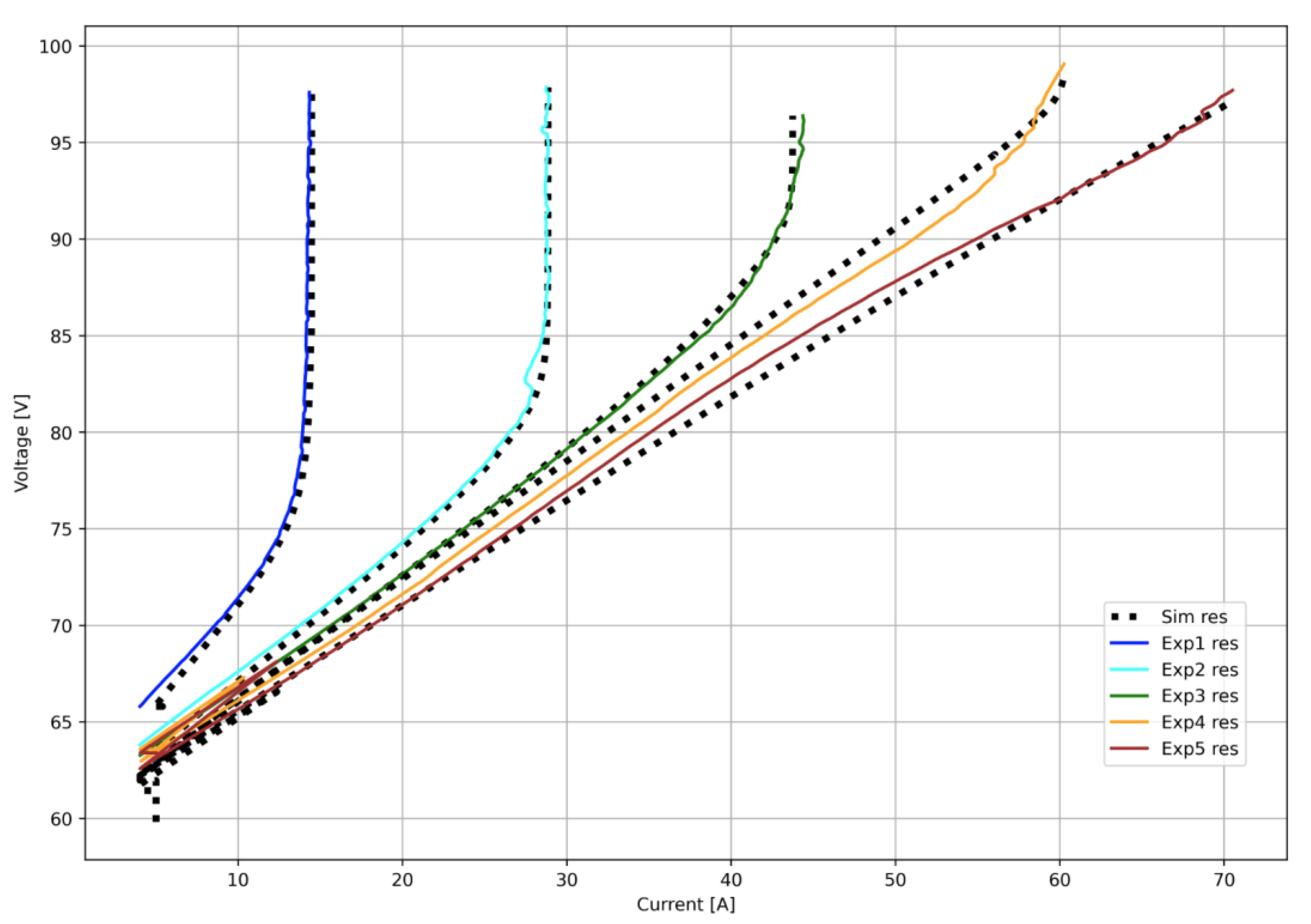
Figure 5.
b. Relative error of the simulated voltage, Eq. (11), for the five selected experiments.
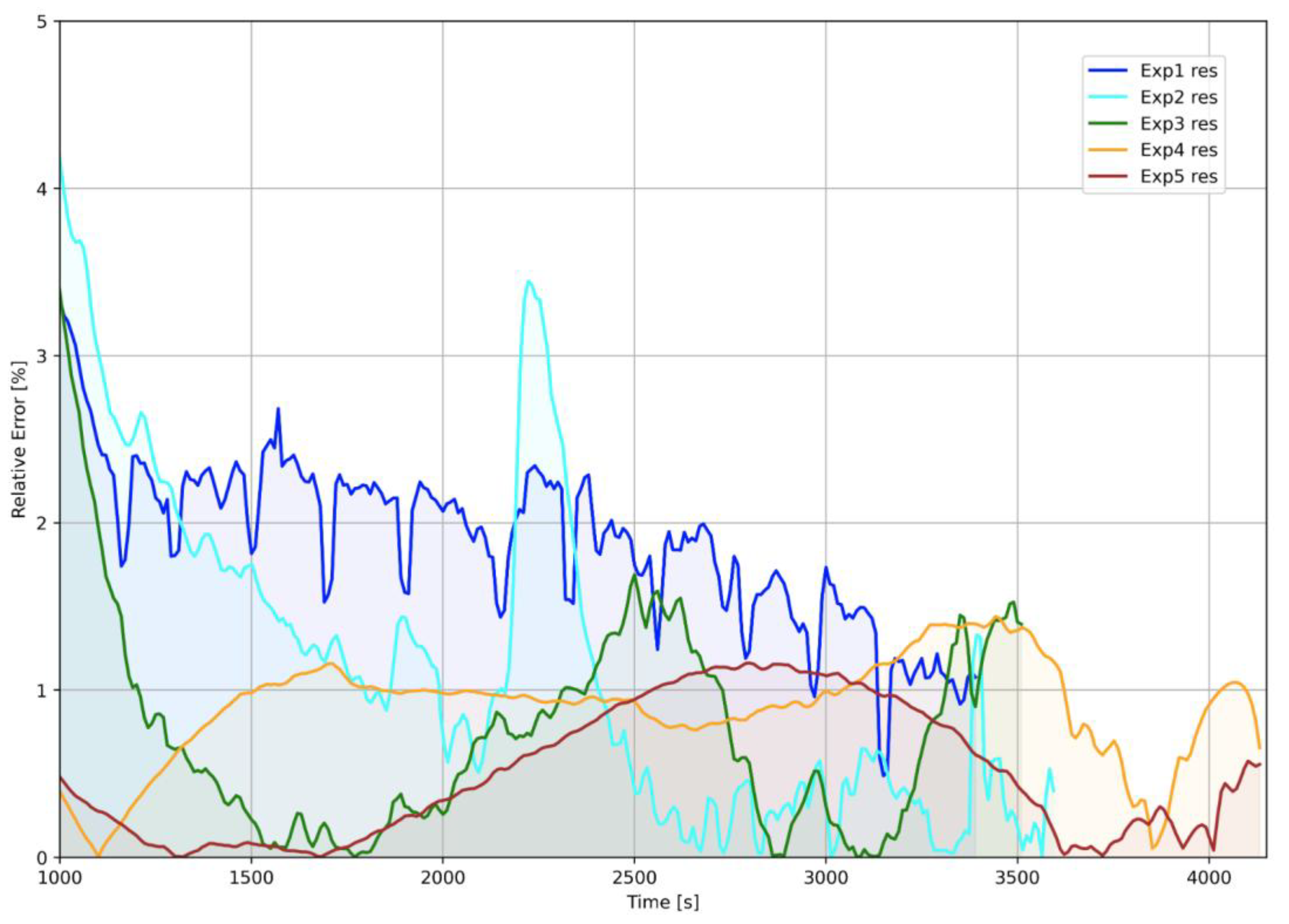
The error is below 3% for the blue curve and below 2% otherwise, apart from the initial points and a sensor anomaly in experiment 2. The calibrated parameters were transferred to the 25 kW configuration, which employs the same cell materials with the active area increased fourfold (80 to 320 cm2) and 80 cells instead of the 70 of the test bench; since the ASR is normalised to area the extrapolation is well founded, while in-plane uniformity and channel pressure drops are treated as second order until pilot data become available. The calibration of the air pre-heater E104, the dominant HEX of the network, is documented in Appendix C.
2.5. Control Architecture
Each functional zone is governed by dedicated control loops (CLs) that keep temperature, pressure, flow rate and level within their bounds, each controlled variable being paired with the manipulated variable acting most directly on it; the safety functions of the HAZOP analysis are omitted. The strategy is the second option of the test campaign [33]: the stack voltage is held at 105.6 V (1.32 V/cell, close to thermoneutral) by an ideal source (CL1); the steam flow is fixed per state (CL2); and the current is tracked by acting on the stack temperature through CL7 and CL8, two cascades in which an outer PI compares the measured current with the PV-derived target and outputs a temperature reference, bounded between 700 °C and the limits of the test campaign, 780 °C for the air at the stack inlet and 800 °C for the fuel heater outlet, ramped at 0.05 K/s and enforced by an inner PI on the electric heaters. Because the ASR decreases with temperature, Eq. (6), raising the inlet temperatures at constant voltage raises the current. The PI gains were tuned with the Ziegler–Nichols method [30,31,32]. Three rules coordinate the loops with the thermal state of the stack: the references are floored at 10 K below the cell temperature of the central segment, so that the inlet gases never cool the stack faster than its own losses allow, the offset being smaller than the ΔT setpoint of CL6; the full-load steam level is held as long as either the current target or the measured current (30 s filter, 10 A hysteresis) exceeds 185 A, so that steam is never reduced ahead of the current; and the direct stack heater is controlled by a PI on the cell temperature (SH), with the fuel-side reference of CL7 as setpoint in Production and 760 °C in HSB and NM, so that it covers the insulation losses when the stack is disconnected and stays idle while the electrochemical heat suffices. The ten loops are listed in Table 2.
2.6. Supervisory State Machine and PV-Driven Operation
Transitions between the states are coordinated by a supervisory layer implemented with the Modelica StateGraph library (Figure 6a). The driving signal is the capacity factor CF = P_PV/P_PV,ref, with P_PV,ref = 26 kW, passed through a slew-rate limiter of 0.005 s−1 to obtain the filtered value CF_f, which removes the chattering of short cloud passages. Two nominal thresholds, CF = 0.10 between NM and HSB and CF = 0.30 between HSB and Production, are widened into hysteresis bands: the plant leaves NM for HSB when CF_f exceeds 0.25 and returns below 0.02; it leaves HSB for Production above 0.50 and returns below 0.15. The wide upper band means that a producing plant tolerates a halving of the PV power before de-energising the stack and sets the minimum depth of a cloud event able to cause a Production–HSB cycle; the narrow lower band keeps the plant in HSB while any significant irradiance is available. Every shut-down or start-up passes through HSB, where steam flow and stack temperature are brought to the values of the next state. The setpoints issued by each transition are listed in Appendix B (Table B1).
Within Production the current target I_target is scaled linearly with CF_f between I_min = 150 A, assigned at the nominal threshold CF_HSB→P = 0.30, and I_max = 256 A, reached at CF_ref = 0.70, Eq. (12); below the lower bound the target is held at 150 A, and in HSB and NM the stack is disconnected.
Figure 6b summarises the signal flow of the supervisory layer. All setpoints pass through slew-rate limiters, so that no transition reaches a loop as a step: 0.2 A/s on the current target (150 to 256 A in about 530 s, consistent with the provider-recommended ramps), 2e-6 kg/s2 on the steam setpoint, 1e-7 and 1e-6 kg/s2 on the make-up and recirculation setpoints, and 0.05 K/s on all temperature references. The sweep-air loop CL6 is handled by the supervisory layer: in HSB and NM no electrochemical heat is released and a ΔT setpoint is meaningless, so the air flow is commanded to the blower minimum (0.002 kg/s) and the controller is frozen with its reference equal to the measurement; the same freezing applies in Production whenever the air heater is saturated (Section 3.4). The PV profile acts as a dispatch signal for a grid-connected plant: the electrical balance is not closed, since the stack absorbs 27 kW at full load against a PV peak of 27.6 kW and the auxiliaries add 3.6 kW.
2.7. Simulation Scenarios and Performance Indicators
Two consecutive days are simulated from 07:00 of the first day to 23:00 of the second (40 h). The first day uses an idealised clear-sky PV profile (hourly values, peak 27.6 kW at 12:00); the second modulates the same envelope with five events chosen to exercise the supervisory logic (Figure 7): two short morning passages (10 and 15 min at 50%), which must not trigger a state change, a 45 min overcast front at midday (10%), which drives the capacity factor below the exit threshold, one short afternoon passage and diffuse cover from 16:30 (40%). A dawn ramp from 05:00 links the two days so that the NM–HSB–Production start-up is captured. The fluctuation is applied on the electrical side only, the HTF temperature being held by the thermal store; the heating-up of the plant is outside the scope, and the simulation is initialised in Production at 07:00.
The indicators are the hydrogen production, the total electrical power and the specific electricity consumption CS. The electrical power collects the stack, the fuel, air and stack heaters, the chiller duty converted with a coefficient of performance of 3, the recirculation blower (compression work divided by the motor efficiency η_m, Appendix G) and the sweep-air blower:
The instantaneous CS is reported only while hydrogen is produced; the daily value CS_day is the ratio of the integrals over the whole day, standby and night included. The sweep-air blower power uses the pressure drop of the modelled air network, an air density of 1.17 kg/m3 and efficiencies of 0.55 and 0.90, and is a lower bound.
3. Results and Discussion
3.1. Clear-Sky Day and Control Loop Behaviour
Figure 8 summarises the two days at 105.6 V. On the clear-sky day the plant is in Production from 07:00, when the initial capacity factor of 0.33 exceeds the entry threshold, until 17:56, in HSB until 18:54 and in NM afterwards. The current follows the PV signal with the 0.2 A/s ramp, on the 256 A plateau from 08:39 to 15:37; hydrogen production peaks at 0.77 kg/h for a daily total of 7.85 kg. The inlet temperatures on both sides are set by the cascades: 774 °C at full load, 706 °C at the end of the evening ramp-down, when the references rest on their 700 °C bound, and 760 °C in HSB and NM; the cell temperature follows within a few kelvin. The air panels show the thermal balance of the strategy: at 1.32 V/cell the electrochemical heat at 256 A, about 0.8 kW, matches the insulation losses (860 W), the measured air ΔT settles at 12.7 K, below the 15 K setpoint, and CL6 keeps the air flow at the blower minimum throughout; the current is tracked through the inlet temperatures alone.
On the plateau the stack absorbs 27.0 kW and the auxiliaries 3.6 kW: 2.6 kW in the fuel heater, which raises the steam from 133 °C beyond what E103 recovers, 0.8 kW in the chiller (2.4 kW of cooling at a COP of 3) and 0.2 kW in the air heater; the stack heater is idle on the plateau and delivers up to 2.3 kW for a few minutes at start-up and re-entries. The sweep-air blower requires 2–21 W and contributes less than 0.01 kWh/kg to CS. The instantaneous CS is 39.8 kWh/kg on the plateau and 41 kWh/kg at the end of the ramp-down. Over the clear-sky day the plant consumes 346 kWh for 7.85 kg, a daily CS of 44.1 kWh/kg, of which the night accounts for 28 kWh at 2.4 kW (0.8 kW fuel heater, 0.75 kW stack heater, 0.45 kW air heater, 0.3 kW chiller) against 840 W of insulation losses, the balance being carried away by the night-mode gas flows; the value is consistent with the 38.7 kWh/kg at design point of the 100 kW module [24], the difference being due to ramps, standby and auxiliaries.
Figure 9 shows the remaining loops on the clear-sky day. CL2 tracks the two steam levels with valve openings of 73 and 91% and closes the valve at the transition to NM; CL3 holds the drum pressure within 5 mbar of 3 bar with an HTF flow of 0.04–0.10 kg/s; CL4 produces the sawtooth of the drum level between 0.17 and 0.19 m with a period of about 160 min. CL5 keeps the recirculated flow at 0.03 g/s in Production and 0.63 g/s in NM, the make-up loops dose 0.02 g/s of hydrogen in HSB and 0.07 g/s of forming gas in NM, and the recirculation blower (CL10, not shown) runs at pressure ratios of 1.02–1.20 with 9–54 W electrical. CL9 holds the 50 mbar minimum differential with the back-pressure valve at 13% in Production and 17% in NM, the transient minimum of 21 mbar occurring at the entry into HSB. The stack heater loop is idle while the cascades hold the stack at 774 °C, delivers a 2.3 kW pulse at the transition to HSB, when the reference returns to 760 °C from 713 °C, and settles at 0.75 kW in NM.
Figure 10 shows the cascades CL7 and CL8 over the two days. On the clear-sky day the current is within 3 A of its target on average in Production and lags by up to 20 A during the evening ramp-down, when the references fall at 0.05 K/s and, floored at 10 K below the cell temperature, can only follow the natural cooling of the stack. The references on both sides coincide, from 774 to 700 °C, and are followed by the inner loops within 4 °C; the fuel heater delivers 2.6 kW and the air heater 0.2 kW at full load, and neither approaches its limit. At the start of the simulation the stack, initialised at 760 °C, delivers 243 A against a target of 150 A: the cascades lower the references to 700 °C within 20 min and the current meets the rising target at 07:41 without overshoot. Outside Production the references are replaced by the 760 °C maintenance value and the outer-loop error is nulled, so that no wind-up occurs. On the intermittent day the cloud passages, which lower the target to 169 A, are followed with deviations of up to 30 A, because the two ramp limits are not commensurate: a change of 87 A takes 7 min, the corresponding 35 °C takes 12 min. At the re-entry at 13:22 the current reaches the target at 13:31 without overshoot, the stack heater contributing 2.2 kW for the first minutes; with a stack of negligible thermal capacity the same re-entry produces an overshoot beyond 300 A. The two outer loops act on the same error with independent integrators and coincide within 2 °C here; a single outer loop feeding both references would remove the ambiguity by construction.
3.2. Sensitivity to the Stack Voltage
At constant voltage the thermal balance of the stack depends on the voltage directly: at the thermoneutral value, the electrochemical heat is zero, above it the stack is exothermic and below it endothermic. The 105.6 V (1.32 V/cell) of the test campaign [33] was therefore tested against 102.4 and 104.0 V (1.28 and 1.30 V/cell) and 108.0 and 110.4 V (1.35 and 1.38 V/cell) on the two-day scenario (Figure 11, Table 3). The three lower voltages complete the two days with practically unchanged hydrogen production and consumption, 13.91–14.07 kg and 43.8–44.0 kWh/kg, because the cascades reach the supervisory target at every voltage by adjusting the stack temperature. What changes is the thermal operating point. At 105.6 V the stack runs at 774 °C with the stack heater idle; at 104.0 V the cascades raise it to 780 °C and the stack heater supplies 0.5 kW on the plateau; at 102.4 V the air-side reference sits at its 780 °C bound for 7.4 h, the fuel side compensates at 790 °C, the cell temperature reaches 786–790 °C, above the 780 °C upper limit of the nominal range [33], and the stack heater supplies 1.0 kW on the plateau and 34 kWh over the two days against 18 kWh at 105.6 V. The lower end of the feasible window is thus set by the stack temperature limit and lies between 1.28 and 1.30 V/cell.
The two higher voltages fail by the same mechanism. At 108.0 V the current delivered by the stack at 760 °C exceeds the target from the first minutes and the cascades bring the references to their 700 °C bound within 20 min; the temperature lever is then exhausted while the current is still above the target, and the current settles at the value that the steam supply can sustain at 100% utilisation, 201 A on the partial-load level and 343 A on the full-load level. The last segments of the channel run dry, the concentration overvoltage of Eq. (3) diverges, and the heat released at 1.35 V/cell and 343 A exceeds what the sweep air can remove at the blower maximum: the cell temperature rises without bound, 830 °C at 08:00 and above 1000 °C by 09:50, until the steam-side properties leave their validity range. At 110.4 V the anode channel dries within the first hour. Constant-voltage operation is therefore feasible only within a narrow window, about 1.30–1.33 V/cell with the present steam levels, and above it the strategy requires a protection it does not contain, either a current limiter acting on the voltage, as in the first option of the test campaign, or a steam feed-forward on the measured current. The steam-level rule of Section 2.5 prevents steam starvation during the evening ramp-down but cannot cover a voltage at which the current exceeds the full-load steam supply. The sweep-air setpoint of 15 K, selected through a preliminary sensitivity over 5–25 K with a stack of negligible thermal capacity, is retained: with 25 kJ/K the loop stays at the blower minimum at all feasible voltages, so that the setpoint acts as an upper limit on the stack exothermicity.
3.3. Sensitivity to the Stack Thermal Capacity
The stack thermal capacity of 25 kJ/K is a literature-based estimate (Appendix D) and sets the pace at which the temperature-tracking strategy can act. Its influence was assessed at 105.6 V with 6.25, 12.5, 25 and 50 kJ/K (Figure 12, Table 4). The strategy completes the two days at every value, with the sweep-air loop at the blower minimum and the air heater below 1 kW, and the specific consumption is unchanged, 43.7–43.9 kWh/kg. The capacity changes the lag between the current and its target: on the first morning the current meets the target at 07:23 with 6.25 kJ/K and at 07:56 with 50 kJ/K, and the cloud passages are followed with deviations of 20 and 45 A. The evening ramp-down is the most sensitive event, because the stack can only cool at the rate of its insulation losses once the references have reached their floor: with 6.25 and 12.5 kJ/K the current follows within 7 A, with 25 kJ/K it lags by up to 15 A, and with 50 kJ/K the stack is still at 195 A when the target reaches the 150 A floor and the supervisory layer disconnects it. The hydrogen output rises accordingly, from 13.94 to 14.39 kg, and the stack heater pulses at the transitions grow from 2.0 to 3.8 kW. A stack twice as heavy as assumed here would still be operated safely, but its current could not be brought to the floor at the end of the day by the temperature alone, and the current limiter recommended in Section 3.2 would be needed at the ramp-down as well.
3.4. Sweep-Air Loop Outside Production and its Coordination with the Cascades
Two results on the sweep-air loop emerged from configurations that failed. The first is the requirement to disable CL6 in HSB and NM, absent from the original control specification. With the stack disconnected the air leaves the stack colder than it enters, the measured ΔT exceeds any setpoint and CL6 raises the air flow towards the blower maximum: with the original 0.020 kg/s blower the flow saturates at the entry into HSB and remains saturated all night; with the 0.040 kg/s blower the saturation moves to the heaters, the air heater sitting at its 8 kW limit while the stack inlet falls to 634 °C and the night-time heating demand reaches 28 kW. These figures were obtained with the thermal capacity of the original stack model, but the night-time saturation is a steady-state condition independent of the inertia. Holding the air flow at the minimum outside Production keeps the stack at 760 °C with 2.4 kW: the sweep-air loop is a production-state controller whose activation must be a supervisory decision.
The second result appeared when the stack thermal capacity was corrected from the per-cell value of the original model (312 J/K for the lumped stack) to 25 kJ/K, before the floor on the references and the stack heater were introduced. With a stack that no longer follows its inlet temperatures within seconds, the references fell below the stack temperature during the evening ramp-down; the sweep air entered the stack colder than the cells, the measured ΔT exceeded the setpoint, CL6 opened the air flow to the blower maximum, the air heater saturated at 8 kW, and the stack, disconnected shortly after, lost the 700–830 W of its insulation losses that neither the gas flows nor the saturated heater could return: it cooled below 700 °C during the first night and the plant did not recover. The three rules of Section 2.5 and Figure 6b remove the mechanism, and with them the two days are completed with the air flow at the minimum and the air heater below 1.4 kW at every voltage and thermal capacity of Section 3.2 and Section 3.3. The lesson holds for any temperature-tracking strategy: the loops that heat the stack and the loop that cools it must be coordinated with the stack temperature itself, otherwise they work against each other through the stack thermal inertia.
3.5. Intermittent-Cloud Day and Supervisory Behaviour
The second day of Figure 8 tests the supervisory logic. The start-up follows the intended sequence, NM to HSB at 06:57 and HSB to Production at 07:43. The short cloud passages reduce the target to 169 A without leaving Production, the filter and the hysteresis band absorbing them as intended. The midday front drives the capacity factor below 0.15: the plant enters HSB at 12:34, after the current has ramped down to 150 A, and returns to Production at 13:22, an excursion of 48 min; the diffuse afternoon cover brings the exit from Production forward to 17:05 and the entry into NM to 18:40. Hydrogen production is 6.22 kg against 7.85 kg on the clear-sky day, for 185 against 225 kWh of PV energy, and the daily CS of 43.5 kWh/kg is practically equal. The steam, pressure, level and recirculation loops behave as on the clear-sky day at every transition. The two re-entries (07:43 and 13:22) are the most demanding events: the stack, connected at 105.6 V while at 760 °C, delivers at once about 200 A against a target restarting from 150 A; the cascades lower the references towards 700 °C, the stack heater delivers a 2.2 kW pulse when the references turn upwards again, and the current meets the target within 9 min without overshoot. The air ΔT, negative in HSB, returns below the setpoint within minutes, so that CL6 stays at the minimum and the air heater below 0.8 kW. The cell temperature stays between 728 and 776 °C, within the 680–780 °C window, with no oscillatory behaviour. These results complement the steady-state optimisation of [24], which identified the anode air flow as the parameter governing thermal management: dynamically, the air path is the binding constraint during the transitions and outside production, where the supervision of the loop, rather than the blower size, decides whether the plant can be held hot at an acceptable cost.
4. Conclusions
An equation-based dynamic model of the complete BoP of the 25 kW PROMETEO solid oxide electrolyser has been developed in Modelica, with a stack model validated against 5 kW polarisation data within 3% and scaled to 25 kW as a preliminary estimate. The ten-loop constant-voltage, temperature-tracking strategy and a PV-driven supervisory state machine with hysteresis were verified over a clear-sky and an intermittent-cloud day. With the stack thermal capacity of 25 kJ/K and the direct stack heater of the pilot, the stack is thermally neutral at 1.32 V/cell: the sweep-air loop rests at the blower minimum, the current is tracked through the inlet temperatures alone, and the specific consumption is 39.8 kWh/kg at full load and 44 kWh/kg on a daily basis. The feasible voltage window is narrow: at 1.28 V/cell the stack must be held above its 780 °C limit, at 1.35 V/cell and above the current becomes steam-limited and the stack overheats, so that constant-voltage operation requires a current or steam protection that the strategy does not contain; the same protection is needed at the evening ramp-down for a stack heavier than 25 kJ/K, whereas hydrogen output and consumption are otherwise insensitive to the capacity over a factor of eight. The principal design outcome concerns the sweep-air loop: kept active in hot standby and night mode, or in production with references below the stack temperature, it drives blower and heaters into saturation and cools the stack; holding the air flow at its minimum outside production, flooring the references at the stack temperature and freezing the loop while the air heater is saturated keep the stack at temperature with 2.4 kW at night. The supervisory logic handled the cloud-induced transitions, including a 48 min excursion to hot standby, without loss of thermal control.
Three developments follow: a current limiter or a steam feed-forward on the measured current, so that the strategy remains safe outside the window identified here, with a single outer loop feeding both temperature references; measured PV and solar-thermal time series with an explicit model of the molten-salt storage and the closure of the electrical balance; and the cross-validation of the framework against the 25 kW pilot, with degradation models added as operating hours accumulate.
Acknowledgments
This research was funded by the Fuel Cells and Hydrogen 2 Joint Undertaking under grant agreement No. 101007194 (PROMETEO). This Joint Undertaking receives support from the European Union’s Horizon 2020 research and innovation programme, Hydrogen Europe and Hydrogen Europe Research.
Conflicts of Interest
Author Nirmala was employed by the company Modelon AB. The remaining authors declare that the research was conducted in the absence of any commercial orfinancial relationships that could be construed as a potential conflict of interest.:.
Abbreviations
| Symbol | Meaning |
| ASR | Area-specific resistance |
| BoP | Balance of plant |
| CF, CF_f | Capacity factor of the PV plant, raw and filtered |
| CL | Control loop |
| CS | Specific electricity consumption |
| HSB | Hot standby |
| HTF | Heat transfer fluid |
| NM | Night mode |
| PV | Photovoltaic |
| RES | Renewable energy sources |
| SH | Stack heater control loop |
| HEX | Heat exchanger |
| SOEC | Solid oxide electrolysis cell |
| TES | Thermal energy storage |
| WKO | Water knock-out |
Appendix A. BoP Model Components

Table A1.
BoP model components and modelling approach (numbering as in Figure 2 of the main text).
Table A1.
BoP model components and modelling approach (numbering as in Figure 2 of the main text).
| No. | Component | Modelling approach |
|---|---|---|
| 1 | PK104: SOEC stack module | 1D, N = 5 volumes; electrochemical cell model, anode/cathode channels, insulation heat losses |
| 2 | E102: steam generator | Shell-and-tube gas/two-phase exchanger, lumped-pressure pipes, dynamic wall |
| 3 | E104: air pre-heater | Distributed counter-flow gas/gas exchanger, N = 3, dynamic wall |
| 4 | E103: feed/effluent HEX | Distributed counter-flow gas/gas exchanger, N = 3, dynamic wall |
| 5 | EK101: feed electric heater | Prescribed heat flow, PI-controlled (CL7) |
| 6 | EK102: electric air heater | Prescribed heat flow, PI-controlled (CL8) |
| 7 | Chiller | Pipe with constant heat-transfer coefficient and prescribed cooling duty (P control) |
| 8 | WKO: water knock-out | Lumped condensing separator (0D) |
| 9 | Back-pressure valve | Algebraic valve, opening from CL9 |
| 10 | Recirculation blower | Prescribed pressure ratio and isentropic efficiency, no characteristic map (CL10; Appendix E) |
| 11 | Steam lamination valve | Algebraic valve, opening from CL2 |
| 12 | E101: demi-water pre-heater | Lumped economiser |
| 13 | Three-way valve | Algebraic split valve, opening from CL5 |
| 14 | MX101: mixer | Lumped adiabatic mixing volume |
| – | Steam drum | Two-phase drum with metal thermal mass (0D) |
| – | Air blower (sweep air) | Ideal mass-flow source bounded at 0.002–0.040 kg/s; electrical power estimated from the network pressure drop, Eq. (15) |
Appendix B. Transition Logic of the Supervisory State Machine
Table B1.
Transition logic of the supervisory state machine (CF_f: filtered capacity factor; nominal thresholds CF = 0.10 between NM and HSB and CF = 0.30 between HSB and Production).
Table B1.
Transition logic of the supervisory state machine (CF_f: filtered capacity factor; nominal thresholds CF = 0.10 between NM and HSB and CF = 0.30 between HSB and Production).
| Transition | From → To | Condition | Hysteresis | Setpoints issued to the control loops |
|---|---|---|---|---|
| tr_endNightMode | NM → HSB | CF_f > 0.25 | Nominal + 0.15 | Steam flow to the HSB level (CL2, 1.50 g/s); forming-gas purge stopped and H2 make-up resumed; recirculation to the HSB level (CL5); heater and stack-heater references held at 760 °C; stack disconnected; air flow at the blower minimum. |
| tr_toProduction | HSB → Production | CF_f > 0.50 | Nominal + 0.20 | Stack connected at 105.6 V (CL1); current target from Eq. (12), ramped at 0.2 A/s from 150 A; heater references taken over by the cascades CL7 and CL8 and stack-heater setpoint by the fuel-side reference; CL6 enabled with ΔT = 15 K; steam flow to the level of the current target (CL2). |
| tr_endProduction | Production → HSB | CF_f < 0.15 | Nominal − 0.15 | Current target ramped down to 150 A, then stack disconnected (CL1); heater and stack-heater references ramped to 760 °C; CL6 frozen and air flow ramped to the blower minimum; steam flow to the HSB level; H2 make-up from bottles (CL5). |
| tr_toNightMode | HSB → NM | CF_f < 0.02 | Nominal − 0.08 | Steam flow ramped to zero and lamination valve closed (CL2); forming-gas purge 20/80 H2/N2 and recirculation to the NM level (CL5); heater and stack-heater references held at 760 °C; stack disconnected; air flow at the blower minimum. |
Appendix C. Calibration of the Air Pre-Heater E104
For the first calibration of the air pre-heater E104 the datasheet of the plate heat exchanger supplied for the pilot was considered, although it refers to an air-flow range from 32.4 to 108 kg/h (0.009 to 0.030 kg/s), narrower than the range spanned by the simulations. The datasheet conditions are reported in Table C1.
Table C1.
Plate heat exchanger E104: datasheet conditions at minimum and maximum air flow.
| Quantity | Unit | Minimum flow | Maximum flow |
|---|---|---|---|
| Cold-side pressure | bar(a) | 1.30 | 1.30 |
| Hot-side pressure | bar(a) | 1.04 | 1.04 |
| Cold-side mass flow | kg/s | 0.009 | 0.030 |
| Hot-side mass flow | kg/s | 0.009 | 0.032 |
| Cold-side inlet temperature | °C | 25 | 25 |
| Cold-side outlet temperature | °C | 629 | 667 |
| Hot-side inlet temperature | °C | 734 | 734 |
| Hot-side outlet temperature | °C | 146 | 142 |
| Exchanged heat | kW | 5.75 | 20.47 |
| Cold-side pressure drop | mbar | 3.4–3.5 | 11.6–12.7 |
| Hot-side pressure drop | mbar | 0.9–1.0 | 5.2–5.8 |
| Core volume | l | 9.1 | 9.1 |
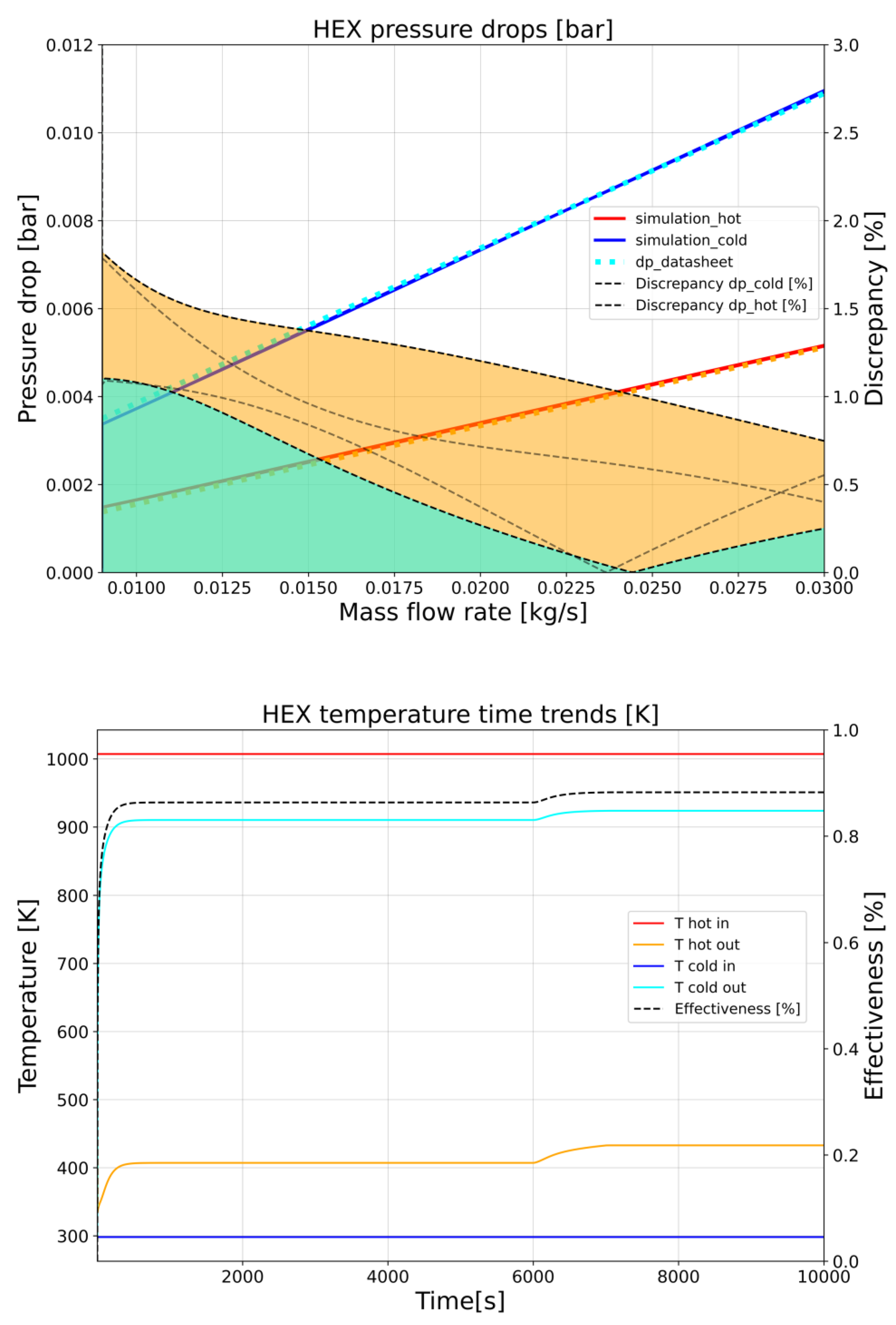
The heat-transfer and friction sub-models of the primary and secondary channels were calibrated against these conditions by adjusting the exchange area and the length of the discretised channels and the correction factors of the heat-transfer and pressure-loss correlations, so that the outlet temperatures and the pressure drops at the two datasheet points were reproduced. Figure C1(a) shows the resulting pressure drops on the two sides as a function of the air mass flow, compared with the datasheet values; the discrepancy stays within 2% over the datasheet range. Figure C1(b) illustrates the thermal response to a ramped increase of the air mass flow from 0.008 to 0.030 kg/s applied between 6000 and 7000 s: following the transient, the cold-side outlet temperature rises by about 15 K and the hot-side outlet by about 25 K, while the effectiveness increases from 86 to 88%, reflecting the improved thermal performance at higher flow rate.
Figure C1.
(a) Pressure drops of E104 on the two sides as a function of the air mass flow, simulation against datasheet values, with the discrepancy on the right axis; (b) inlet and outlet temperatures and effectiveness during the calibration transient.
Figure C1.
(a) Pressure drops of E104 on the two sides as a function of the air mass flow, simulation against datasheet values, with the discrepancy on the right axis; (b) inlet and outlet temperatures and effectiveness during the calibration transient.
Appendix D. Stack Specifications
Table D1 lists the specifications of the 25 kW stack module provided by SolydEra and used in the model.
Table D1.
Specifications and design parameters of the SOEC stack module.
| Specification | Unit | Value |
|---|---|---|
| Full power | kW | 25 |
| Cell voltage at full power (thermoneutral condition) | V | 1.28 |
| Operating voltage in the model (CL1) | V/cell | 1.32 |
| Number of cells | – | 80 |
| Active cell area | cm2 | 320 |
| Insulation thickness (Microtherm) | cm | 13 |
| Insulation density | kg/m3 | 240 |
| Insulation thermal conductivity | W/(m K) | 0.04 |
| Stack thermal capacity used in Eq. (E2), 50 kg at 500 J/(kg K) | kJ/K | 25 |
Appendix E. Cell Energy Balance
The partial pressures of reactants and products are evaluated with Eq. (E1) in each segment of the one-dimensional discretisation, with a penalty function preventing negative values:
T_cell is the cell temperature, connected to the thermal port of the wall (wall.T = T_cell) so that temperature and heat-flow continuity are ensured. Eq. (E2) gives the energy balance of each discretisation element:
where M_cp is the thermal capacity of the lumped stack, 25 kJ/K for 80 cells (50 kg of cell and interconnect material at 500 J/(kg K), consistent with the 0.3–0.5 kJ/K per cell of planar SOC stacks reported in the literature [35,36]), distributed over the N segments, Q_an and Q_cath are the heat flows between the cell and the anode and cathode channels, Q_cell is the heat generated in the i-th element and Q_wall is the heat exchanged with the external environment through the insulation model. The channel heat flows are defined with Eq. (E3), where k_c = 250 W/(m2 K) is the heat-transfer coefficient between fluid and substrate:
The species mass flows through the mass ports are positive for substances entering the element (H2O) and negative for those leaving it (H2, O2). The bulk enthalpy flows of the cathode and anode mixtures follow from the specific enthalpies of the species, Eq. (E4), and Q_cell is obtained from the energy balance of Eq. (E5), where P_cell = V_cell I is the electrical power of the element and V_cell the potential difference between the two electric ports of the elementary cell:
Appendix F. Model Parametrisation
Table F1 compiles the discretisation, geometry, gas volumes and thermal parameters of the BoP components, as set in the model. Values marked with an asterisk are calibration or preliminary values to be confirmed against the as-built pilot.
Table F1.
Discretisation and parametrisation of the BoP model components.
| Component | Discretisation | Geometry and volumes | Thermal parameters |
|---|---|---|---|
| SOEC stack (PK104) | 1D, N = 5 elements per channel | 80 cells × 320 cm2; anode and cathode channels L = 0.11 m, D_h = 1.55 mm, gas volume 16.6 cm3 per channel | Stack thermal capacity 25 kJ/K (50 kg × 500 J/(kg K)) over the five segments; k_c = 250 W/(m2 K); insulation 0.13 m Microtherm on top, bottom and sides (A = 1, 1 and 2 m2), k = 0.04 W/(m K), external convection 12 (top) and 5 (side) W/(m2 K), emissivity 0.04; ASR0 = 0.356 Ω cm2, E_a = 57.7 kJ/mol, α = 0.5 |
| E104 air pre-heater | 1D counter-flow, N = 3 | Exchange area 10 m2 (secondary) and 1 m2* (primary), L = 0.5 m, D_h = 10 mm | Wall mass 0.3 kg*, steady-state wall initialisation; pressure-loss operating point 100 Pa at 0.003 kg/s |
| E103 feed/effluent HEX | 1D counter-flow, N = 3 | Channel L = 1 m, D_h = 20 mm, exchange area 0.1 m2 per side* | Constant heat-transfer coefficient 100 W/(m2 K)*; stainless steel 316L wall |
| E102 steam generator | Shell-and-tube, lumped-pressure pipes | Primary (HTF) L = 0.8 m, D = 20 mm; secondary (water/steam) L = 0.8 m, D = 2 mm | Two-phase heat-transfer coefficients 3000 W/(m2 K); primary 1500 W/(m2 K); standard steel wall |
| Steam drum | 0D two-phase volume | L = 1 m, r_int = 0.50 m, r_ext = 0.51 m | Metal thermal mass from steel density 8000 kg/m3 and c_p 500 J/(kg K); setpoint 3 bar, level 0.18 m |
| E101 economiser | 0D | Lumped water pre-heater at 3 bar | – |
| Chiller | Pipe, lumped | L = 1 m, D = 16 mm, V = 0.20 l | Constant coefficient 800 W/(m2 K); duty set by P control to the WKO inlet temperature; COP 3 for the electrical equivalent |
| WKO / condensing separator | 0D | V = 0.1 m3 | Condensation time constant 2 s |
| Cold-side gas volumes | 0D, N = 2–4 ports | 0.1 m3 (separator outlet), 0.15 m3 (recirculation), 2 l (blower outlet) | Isothermal at 5 °C (cold zone) |
| Pipes to stack (fuel, air) | Pipe, lumped | L = 1 m, D = 20 mm, V = 0.31 l each | Adiabatic |
| Sweep-air blower | Ideal mass-flow source | Range 0.002–0.040 kg/s | Power estimated with η_blower = 0.55, η_motor = 0.90, Eq. (15) |
| Recirculation blower | Prescribed pressure ratio (Appendix E) | – | Isentropic efficiency 0.75; motor and transmission efficiency 0.30 |
| Electric heaters | Prescribed heat flow | – | Limits 8 kW (electrical heater) reference ramp 0.05 K/s |
Appendix G. Recirculation Blower Model
The anode recirculation blower (item 10 of Table A1) is represented by a prescribed-pressure-ratio, prescribed-efficiency model without a characteristic map, since the machine of the pilot has not been characterised yet. The mass flow through the blower is determined by the circuit, namely by the recirculation valve of CL5, and the pressure ratio PR = p_out/p_in is set by CL10 as a feedforward: the delivery pressure is kept above the measured mixer pressure by a margin proportional to the opening command of the recirculation valve (CL5), up to 150 mbar, the ratio being bounded between 1 and 1.35 and filtered with a time constant of 2 s to represent the machine response. The inlet state is evaluated from the enthalpy and composition of the incoming reformate mixture, treated as an ideal gas, and the isentropic exponent γ = c_p/c_v is evaluated at the inlet. The isentropic outlet temperature is obtained explicitly, without an inner iteration,
the isentropic outlet enthalpy h_is is evaluated at the outlet pressure and T_is, and the actual outlet enthalpy follows from the isentropic efficiency η_is = 0.75, all losses being transferred to the gas:
The compression work is obtained from a static energy balance and converted to electrical power with a motor and transmission efficiency η_m = 0.30, a conservative value for the small machine of the pilot to be confirmed against the as-built hardware; this is the term P_c,rec/η_m of Eq. (13):
Flow reversal through the blower is not supported and is asserted; the pressure ratio is bounded below at 1. The outlet composition equals the inlet composition and the blower has no thermal capacity of its own, the downstream volume (Table F1) providing the dynamics of the recirculation line.
References
- Fang, R.; Liang, Y. Control strategy of electrolyzer in a wind-hydrogen system considering the constraints of switching times. Int. J. Hydrogen Energy 2019, 44, 25104–25111. [Google Scholar] [CrossRef]
- Ibrahim, M.H.; Ang, S.P.; Dani, M.N.; Petra, R.; Salam, M.A. Voltage stability assessment for solar photovoltaic penetration using Reactive Power–Voltage and Active Power–Voltage modal analysis. Energy Rep. 2023, 9, 486–493. [Google Scholar] [CrossRef]
- Schaab, K.; Hahn, J.; Wolkov, M.; Stursberg, O. Robust control for voltage and transient stability of power grids relying on wind power. Control Eng. Pract. 2017, 60, 7–17. [Google Scholar] [CrossRef]
- Panwar, N.L.; Kaushik, S.C.; Kothari, S. Role of renewable energy sources in environmental protection: A review. Renew. Sustain. Energy Rev. 2011, 15, 1513–1524. [Google Scholar] [CrossRef]
- Kabir, M.M.; Akter, M.M.; Huang, Z.; Tijing, L.; Shon, H.K. Hydrogen production from water industries for a circular economy. Desalination 2023, 554, 116448. [Google Scholar] [CrossRef]
- Chi, J.; Yu, H. Water electrolysis based on renewable energy for hydrogen production. Chin. J. Catal. 2018, 39, 390–394. [Google Scholar] [CrossRef]
- Zhou, Y.; Li, R.; Lv, Z.; Liu, J.; Zhou, H.; Xu, C. Green hydrogen: A promising way to the carbon-free society. Chin. J. Chem. Eng. 2022, 43, 2–13. [Google Scholar] [CrossRef]
- Nemmour, A.; Inayat, A.; Janajreh, I.; Ghenai, C. Green hydrogen-based E-fuels (E-methane, E-methanol, E-ammonia) to support clean energy transition: A literature review. Int. J. Hydrogen Energy 2023, 48, 29011–29033. [Google Scholar] [CrossRef]
- Li, X.; Raorane, C.J.; Xia, C.; Wu, Y.; Tran, T.K.N.; Khademi, T. Latest approaches on green hydrogen as a potential source of renewable energy towards sustainable energy: Spotlighting of recent innovations, challenges, and future insights. Fuel 2023, 334, 126684. [Google Scholar] [CrossRef]
- Agaton, C.B.; Batac, K.I.T.; Reyes, E.M., Jr. Prospects and challenges for green hydrogen production and utilization in the Philippines. Int. J. Hydrogen Energy 2022, 47, 17859–17870. [Google Scholar] [CrossRef]
- Wang, C.; Walsh, S.D.C.; Weng, Z.; Haynes, M.W.; Summerfield, D.; Feitz, A. Green steel: Synergies between the Australian iron ore industry and the production of green hydrogen. Int. J. Hydrogen Energy 2023, 48, 32277–32293. [Google Scholar] [CrossRef]
- Zaiter, I.; Ramadan, M.; Bouabid, A.; El-Fadel, M.; Mezher, T. Potential utilization of hydrogen in the UAE’s industrial sector. Energy 2023, 280, 128108. [Google Scholar] [CrossRef]
- Zhang, F.; Zhao, P.; Niu, M.; Maddy, J. The survey of key technologies in hydrogen energy storage. Int. J. Hydrogen Energy 2016, 41, 14535–14552. [Google Scholar] [CrossRef]
- Nnabuife, S.G.; et al. The prospects of hydrogen in achieving net zero emissions by 2050: A critical review. Sustain. Chem. Clim. Action 2023, 2, 100024. [Google Scholar] [CrossRef]
- Chen, W.; Sun, C. Recent advances in high temperature solid oxide electrolytic cells. Energy Mater. 2025, 5, 500045. [Google Scholar] [CrossRef]
- Barelli, L.; Bidini, G.; Cinti, G. Air variation in SOE: Stack experimental study. Int. J. Hydrogen Energy 2018, 43, 11655–11662. [Google Scholar] [CrossRef]
- Yin, R.; Sun, L.; Khosravi, A.; Malekan, M.; Shi, Y. Control-oriented dynamic modeling and thermodynamic analysis of solid oxide electrolysis system. Energy Convers. Manag. 2022, 271, 116331. [Google Scholar] [CrossRef]
- Saeedmanesh, A.; Colombo, P.; McLarty, D.; Brouwer, J. Dynamic behavior of a solid oxide steam electrolyzer system using transient photovoltaic generated power for renewable hydrogen production. J. Electrochem. Energy Convers. Storage 2019, 16, 041008. [Google Scholar] [CrossRef]
- Motylinski, K.; Kupecki, J.; Numan, B.; Hajimolana, Y.S.; Venkataraman, V. Dynamic modelling of reversible solid oxide cells for grid stabilization applications. Energy Convers. Manag. 2021, 228, 113674. [Google Scholar] [CrossRef]
- Botta, G.; Romeo, M.; Fernandes, A.; Trabucchi, S.; Aravind, P.V. Dynamic modeling of reversible solid oxide cell stack and control strategy development. Energy Convers. Manag. 2019, 185, 636–653. [Google Scholar] [CrossRef]
- Zhang, R.; Jiang, P.; Zhu, Y. Control-oriented modeling and dynamic behavior analysis of a solid oxide electrolysis cell hydrogen production system. Fuel 2025, 390, 134648. [Google Scholar] [CrossRef]
- Fritzson, P.; Engelson, V. Modelica—A unified object-oriented language for system modeling and simulation. In ECOOP’98—Object-Oriented Programming; Jul, E., Ed.; Springer: Berlin/Heidelberg, Germany, 1998; pp. 67–90. [CrossRef]
- Modelon Impact: Systems Modeling and Simulation Platform. Available online: https://www.modelon.com/modelon-impact/ (accessed on 23 June 2026).
- Barreto, G.; Romero, M.; González-Aguilar, J.; Giaconia, A.; Testi, M. Design point, part load and annual performance analysis of a 100 kW SOEC system integrating a solar steamer under electrolyser operational constraints. Renew. Energy 2026, 256, 124340. [Google Scholar] [CrossRef]
- McBride, B.J.; Zehe, M.J.; Gordon, S. NASA Glenn Coefficients for Calculating Thermodynamic Properties of Individual Species; NASA Glenn Research Center: Cleveland, OH, USA, 2002; Available online: https://ntrs.nasa.gov/citations/20020085330 (accessed on 23 June 2026).
- Modelica: Media.Water.StandardWater. Available online: https://doc.modelica.org/Modelica%204.0.0/Resources/helpWSM/Modelica/Modelica.Media.Water.StandardWater.html (accessed on 23 June 2026).
- Therminol 66 Heat Transfer Fluid. Available online: https://www.eastman.com/en/products/product-detail/71093438/therminol-66-heat-transfer-fluid (accessed on 23 June 2026).
- Sigfridsson, S.; Li, L.; Runvik, H.; Gohl, J.; Joly, A.; Soltesz, K. Modeling of fuel cell hybrid vehicle in Modelica: Architecture and drive cycle simulation. In Proceedings of the 2nd Japanese Modelica Conference, Tokyo, Japan, 17–18 May 2018; pp. 91–98. [Google Scholar] [CrossRef]
- Provatas, V.; Dapontis, S.; Konsolakis, M.; Ipsakis, D. Modeling and control of hydrogen production systems through water electrolysis and RES power. Proceedings 2024, 105, 51. [Google Scholar] [CrossRef]
- Mewada, Y.; Prajapati, S.; Hakani, R. System for PID control and autotuning PID using Ziegler–Nichols method. Influ. Int. J. Sci. Rev. 2022, 4, 249–253. [Google Scholar] [CrossRef]
- Yucelen, T.; Kaymakci, O.; Kurtulan, S. Self-tuning PID controller using Ziegler–Nichols method for programmable logic controllers. IFAC Proc. Vol. 2006(39), 11–16. [CrossRef]
- Huba, M.; Chamraz, S.; Bistak, P.; Vrancic, D. Making the PI and PID controller tuning inspired by Ziegler and Nichols precise and reliable. Sensors 2021, 21, 6157. [Google Scholar] [CrossRef]
- Crespi, E.; Panaccione, F.; Ragaglia, D.; Testi, M. Integration of a solid oxide electrolysis system with solar thermal and electrical energy: A testing campaign for operation and control strategy definition. IET Renew. Power Gener. 2024, 18, 4399–4413. [Google Scholar] [CrossRef]
- Pedregosa, F.; et al. Scikit-learn: Machine learning in Python. J. Mach. Learn. Res. 2011, 12, 2825–2830. [Google Scholar]
- Aguiar, P.; Adjiman, C.S.; Brandon, N.P. Anode-supported intermediate temperature direct internal reforming solid oxide fuel cell. I: Model-based steady-state performance. J. Power Sources 2004, 138, 120–136. [Google Scholar] [CrossRef]
- Petipas, F.; Brisse, A.; Bouallou, C. Model-based behaviour of a high temperature electrolyser system operated at various loads. J. Power Sources 2013, 239, 584–595. [Google Scholar] [CrossRef]
Figure 1.
Process flow diagram of the BoP of the hydrogen production plant.
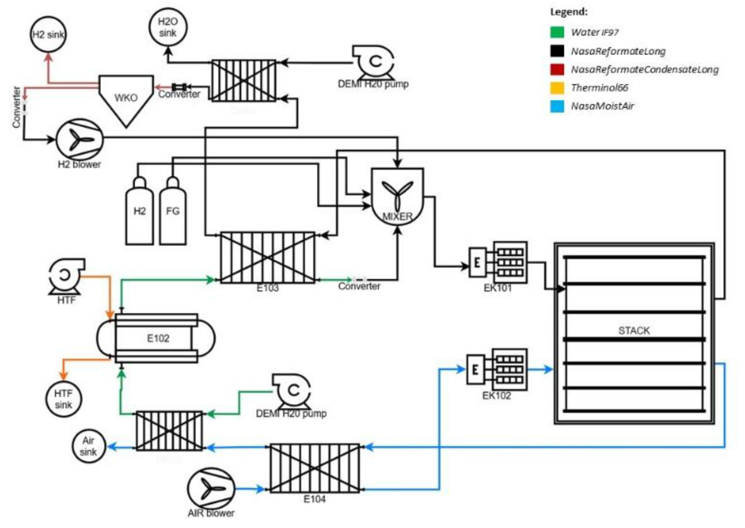
Figure 2.
Layout of the complete model in Modelon Impact.
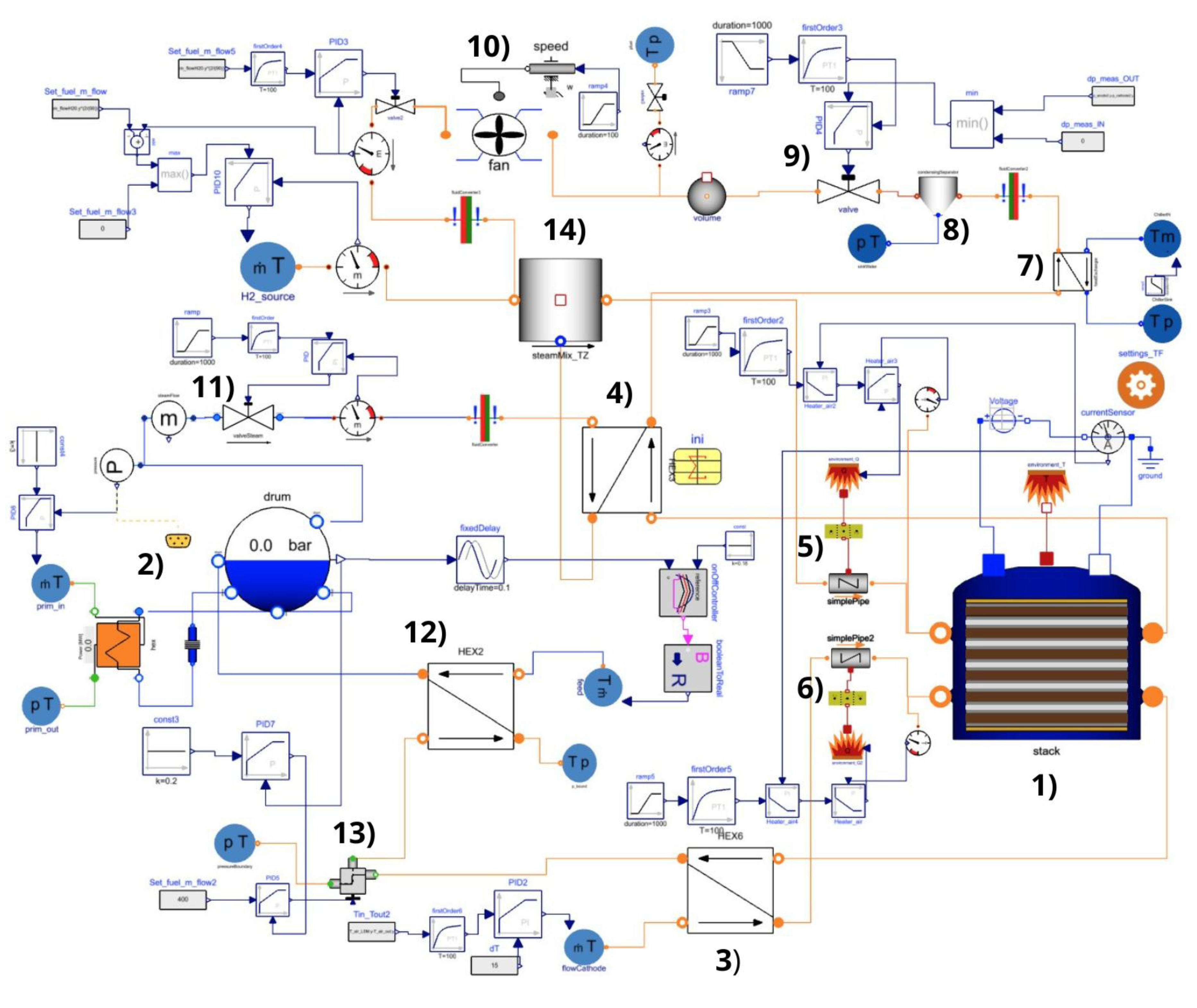
Figure 3.
Elementary cell model.
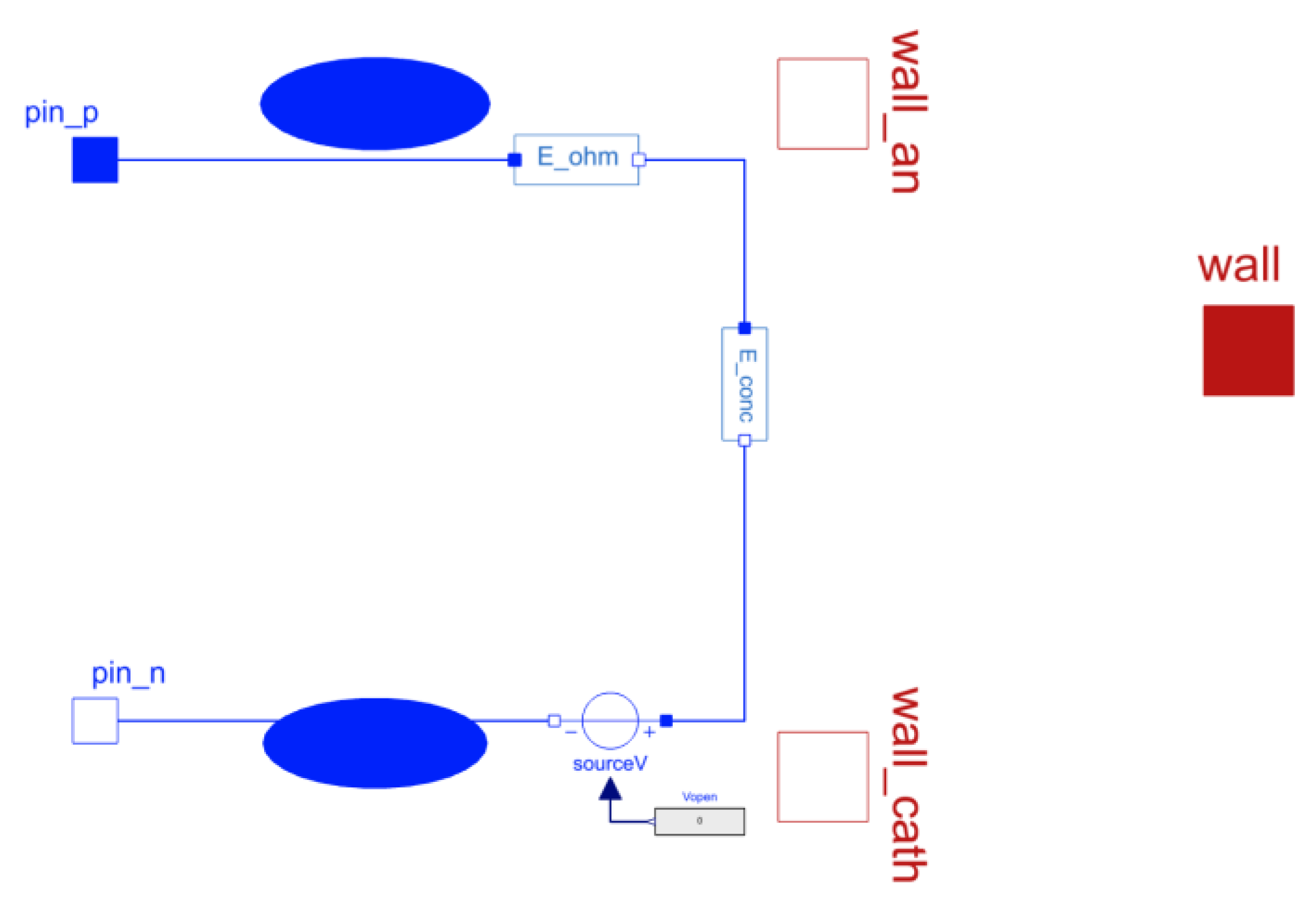
Figure 4.
Experimental voltage versus steam utilisation on the 5 kW test bench, the data set used for the calibration of the stack parameters.
Figure 4.
Experimental voltage versus steam utilisation on the 5 kW test bench, the data set used for the calibration of the stack parameters.
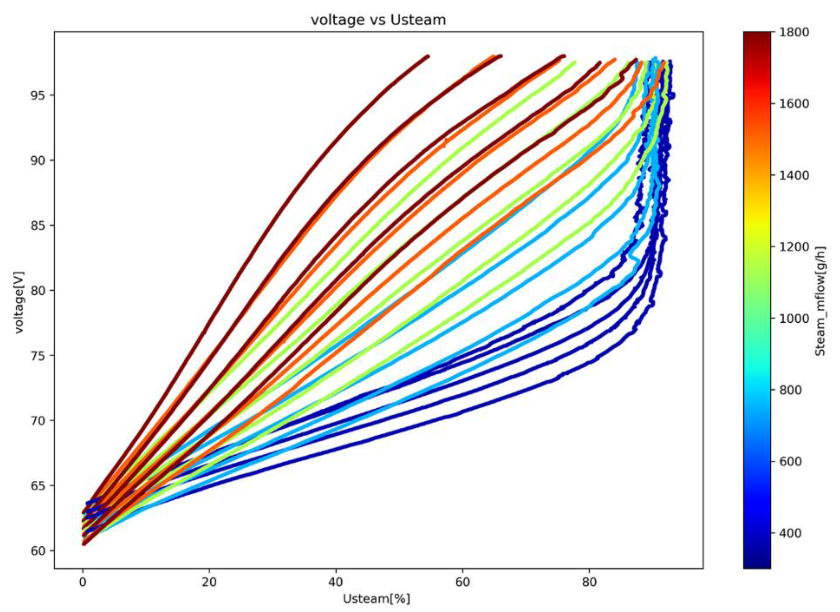
Figure 6.
(a) Supervisory state machine (Modelica StateGraph) with the four signal-driven transitions. (b) Signal flow of the supervisory layer: dispatch signal and state machine (A); current target, cascades, bounds, floor and stack-heater setpoint (B); steam-level rule (C); sweep-air enable rule and air-heater anti-saturation (D). Dashed arrows are signals passed between lanes.
Figure 6.
(a) Supervisory state machine (Modelica StateGraph) with the four signal-driven transitions. (b) Signal flow of the supervisory layer: dispatch signal and state machine (A); current target, cascades, bounds, floor and stack-heater setpoint (B); steam-level rule (C); sweep-air enable rule and air-heater anti-saturation (D). Dashed arrows are signals passed between lanes.
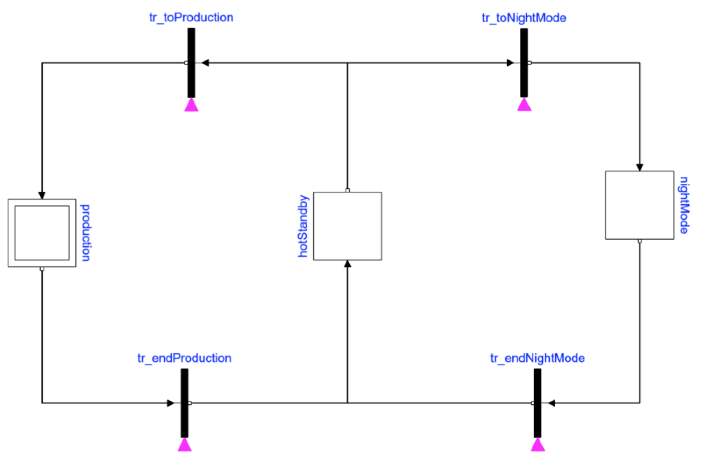
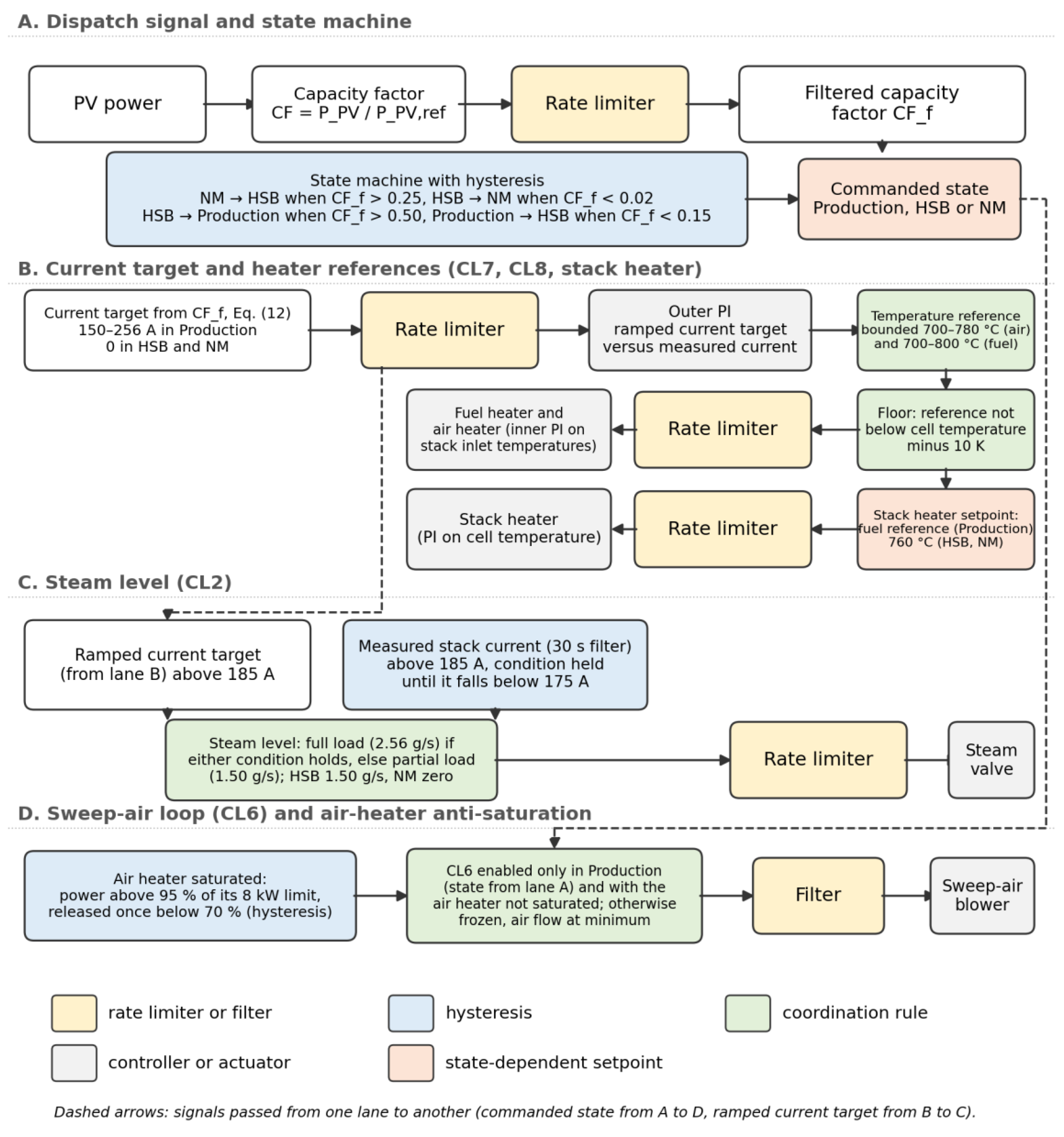
Figure 7.
PV power profile over the two simulated days: idealised clear-sky day followed by the synthetic intermittent-cloud day. Dashed lines mark the state-machine thresholds expressed in PV power.
Figure 7.
PV power profile over the two simulated days: idealised clear-sky day followed by the synthetic intermittent-cloud day. Dashed lines mark the state-machine thresholds expressed in PV power.
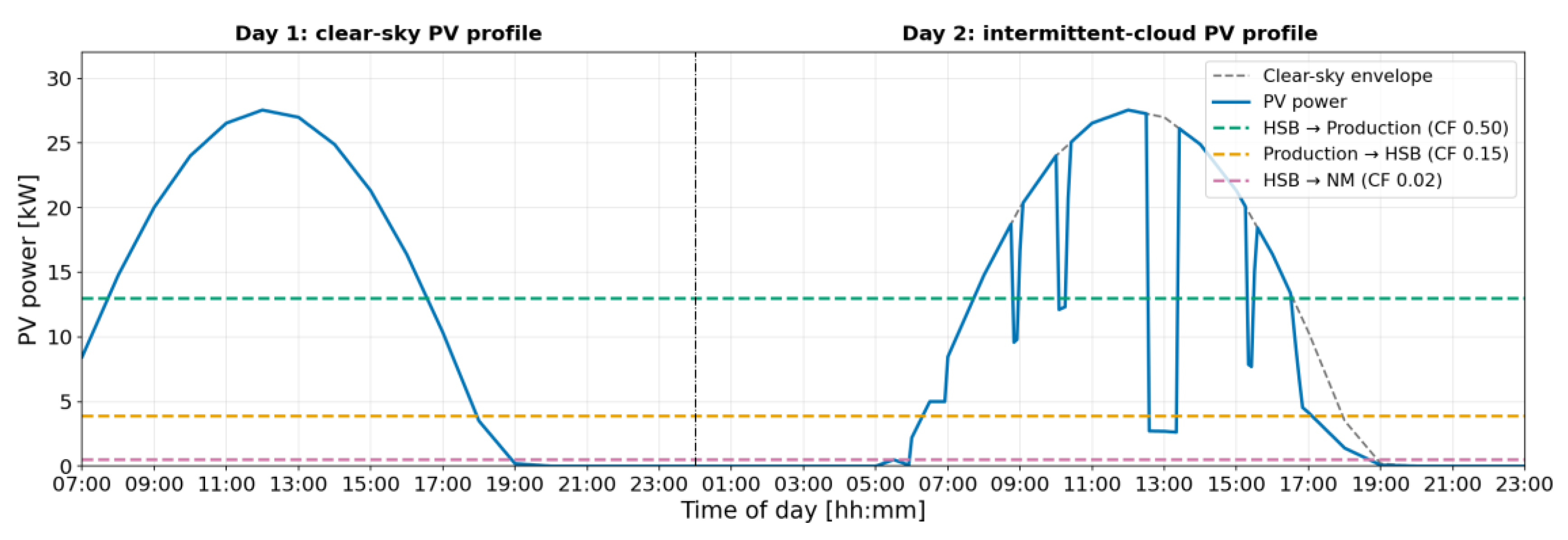
Figure 8.
Two-day simulation at 105.6 V. From top: PV power with supervisory state and thresholds; stack current and hydrogen production; stack inlet temperatures; sweep-air ΔT and air flow (CL6); electrical power of the auxiliaries; specific consumption CS (grey: no hydrogen production).
Figure 8.
Two-day simulation at 105.6 V. From top: PV power with supervisory state and thresholds; stack current and hydrogen production; stack inlet temperatures; sweep-air ΔT and air flow (CL6); electrical power of the auxiliaries; specific consumption CS (grey: no hydrogen production).
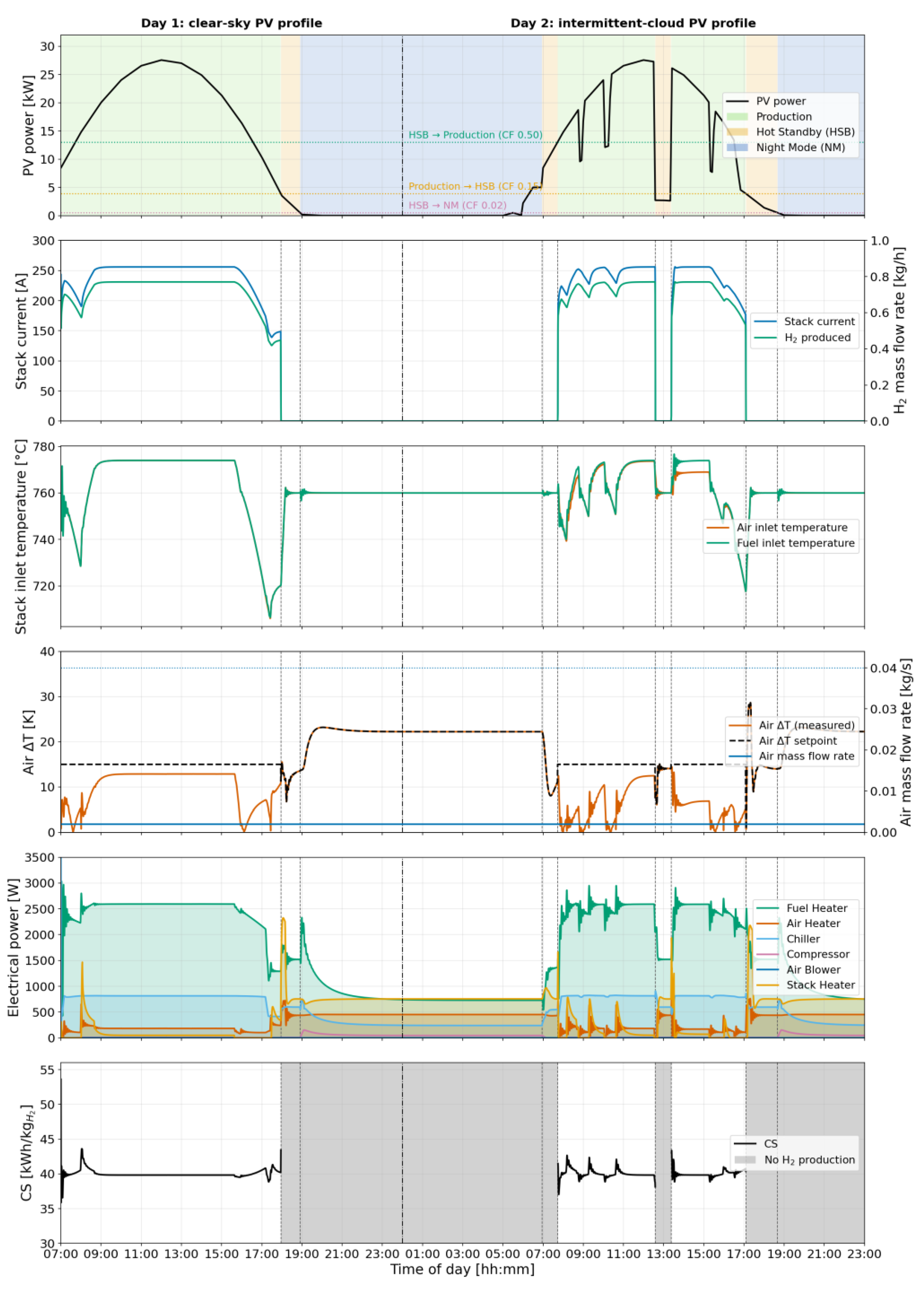
Figure 9.
Control loops CL2, CL3, CL4, CL5 (recirculation and make-up dosing), CL9 and the stack heater loop on the clear-sky day at 105.6 V (setpoints dashed, manipulated variables in red on the right axes).
Figure 9.
Control loops CL2, CL3, CL4, CL5 (recirculation and make-up dosing), CL9 and the stack heater loop on the clear-sky day at 105.6 V (setpoints dashed, manipulated variables in red on the right axes).
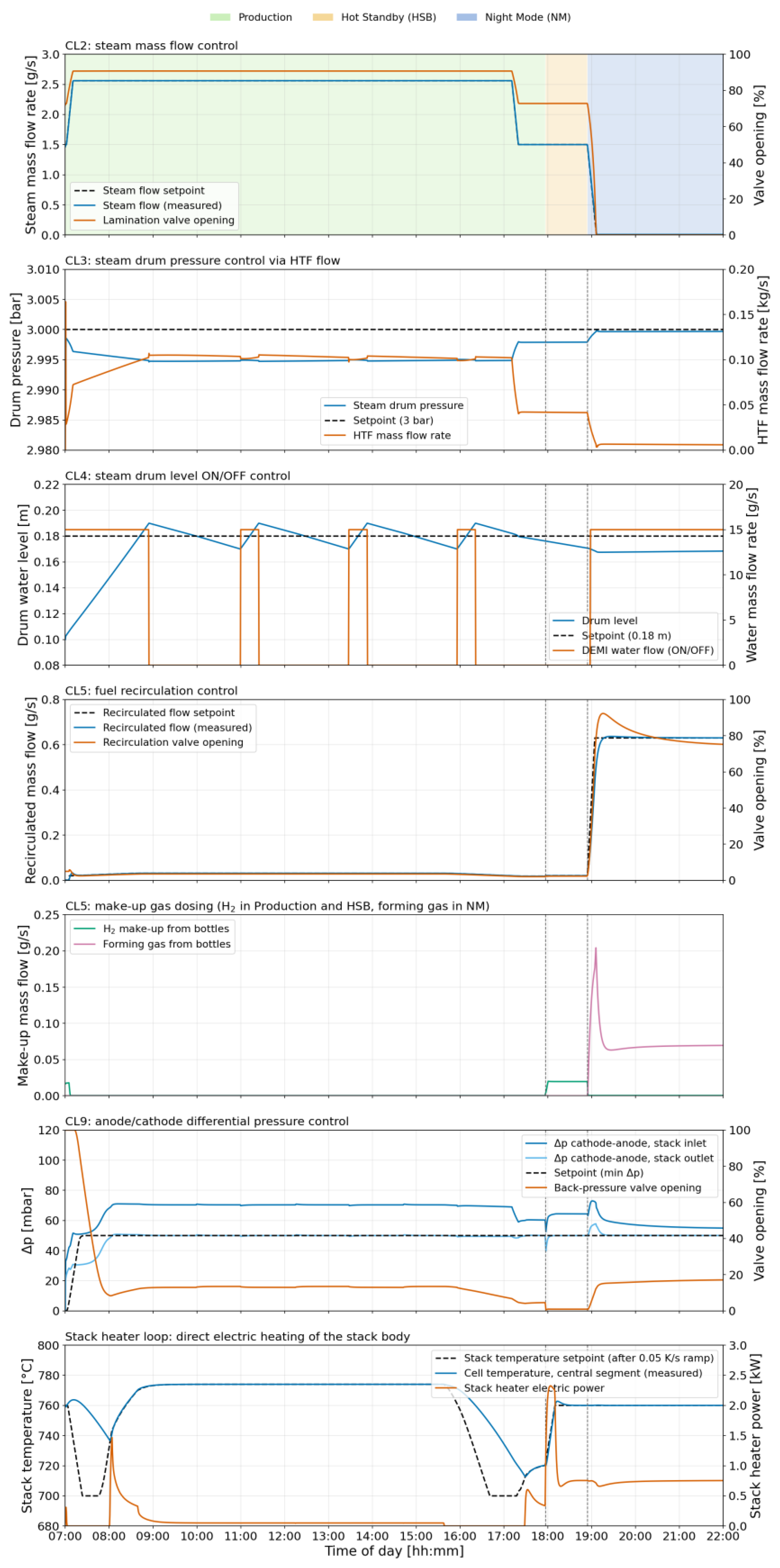
Figure 10.
Current-tracking cascades CL7 and CL8 over the two days at 105.6 V. From top: stack current and its ramped target; temperature references after the 0.05 K/s ramp (dashed) and measured inlet temperatures, with the 700 °C lower bound and the 780 °C (air) and 800 °C (fuel) upper bounds; electric power of the fuel and air heaters.
Figure 10.
Current-tracking cascades CL7 and CL8 over the two days at 105.6 V. From top: stack current and its ramped target; temperature references after the 0.05 K/s ramp (dashed) and measured inlet temperatures, with the 700 °C lower bound and the 780 °C (air) and 800 °C (fuel) upper bounds; electric power of the fuel and air heaters.
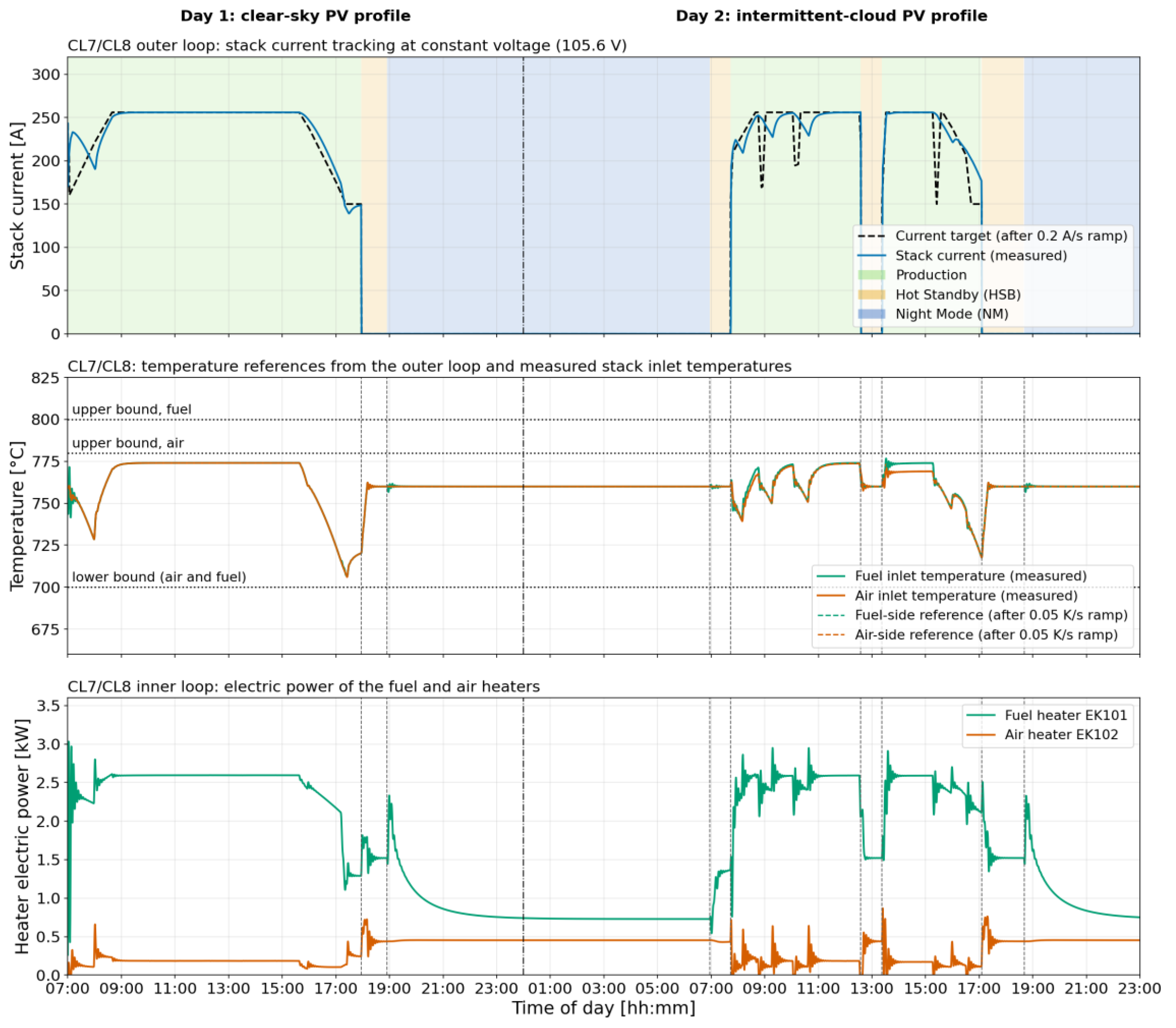
Figure 11.
Sensitivity to the stack voltage (102.4, 104.0 and 105.6 V, i.e., 1.28, 1.30 and 1.32 V/cell) over the two days: stack current with its target; cell temperature of the central segment, with the 780 °C upper limit of the nominal stack range; stack air inlet temperature, with the 780 °C bound of the air-side reference; stack heater power. The runs at 108.0 and 110.4 V terminate on the first morning.
Figure 11.
Sensitivity to the stack voltage (102.4, 104.0 and 105.6 V, i.e., 1.28, 1.30 and 1.32 V/cell) over the two days: stack current with its target; cell temperature of the central segment, with the 780 °C upper limit of the nominal stack range; stack air inlet temperature, with the 780 °C bound of the air-side reference; stack heater power. The runs at 108.0 and 110.4 V terminate on the first morning.
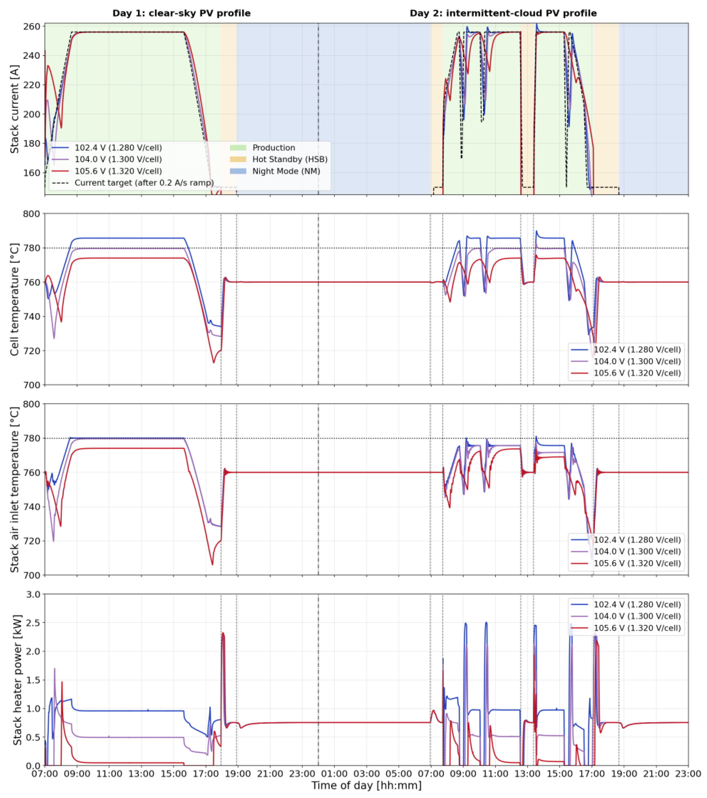
Figure 12.
Sensitivity to the stack thermal capacity (6.25, 12.5, 25 and 50 kJ/K) at 105.6 V over the two days: stack current with its target; cell temperature of the central segment; stack heater power.
Figure 12.
Sensitivity to the stack thermal capacity (6.25, 12.5, 25 and 50 kJ/K) at 105.6 V over the two days: stack current with its target; cell temperature of the central segment; stack heater power.
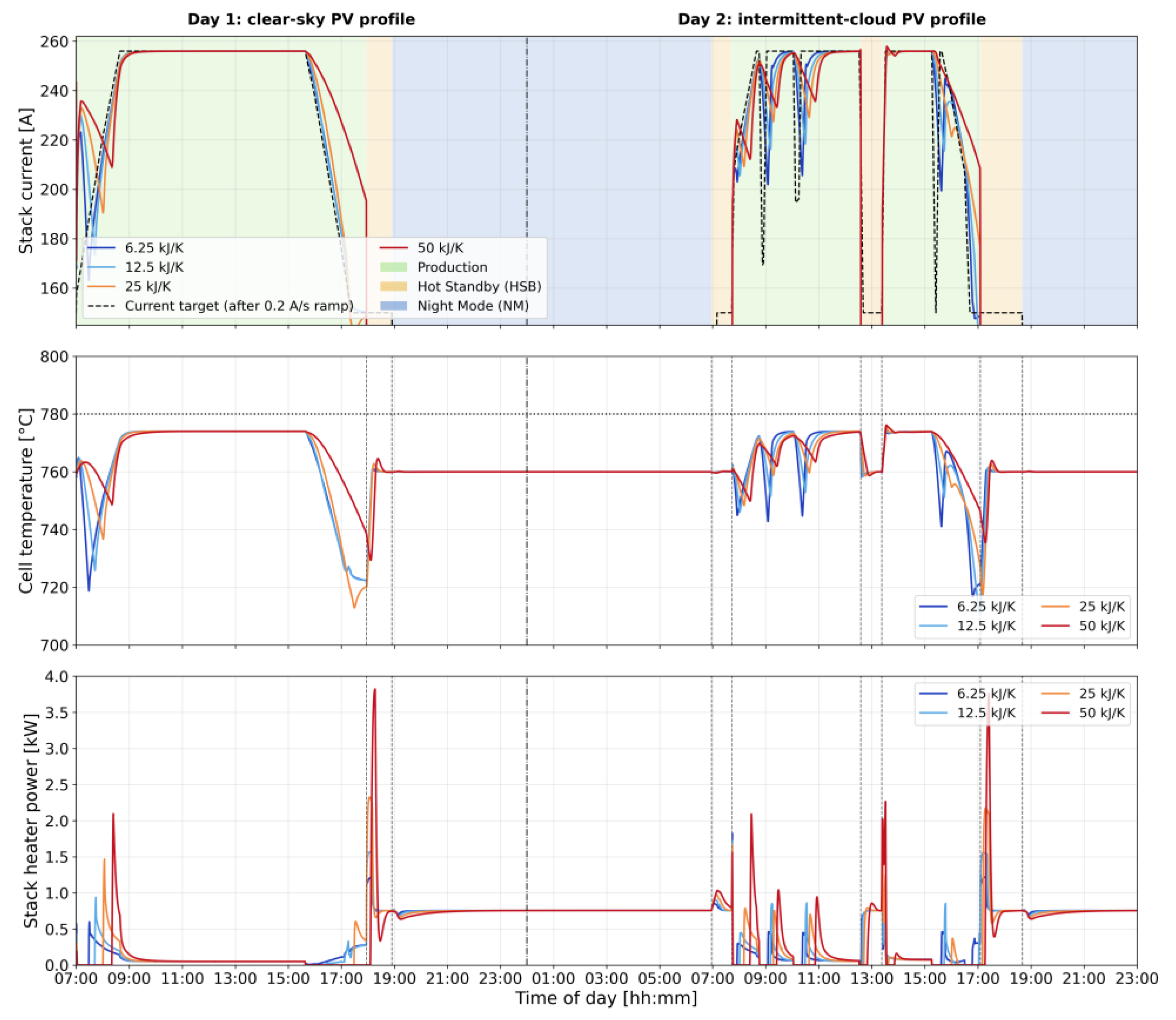
Table 1.
Operating states, cathode feed and electrical condition (volume fractions of the cathode feed; steam utilisation from Eq. (7)).
Table 1.
Operating states, cathode feed and electrical condition (volume fractions of the cathode feed; steam utilisation from Eq. (7)).
| State | Cathode feed (kg/s) | H2 / H2O / N2 (vol. %) | Electrical condition | Current (A) | Steam utilisation (%) |
|---|---|---|---|---|---|
| Production, full-load steam level (target > 185 A) | steam 2.56e-3 + H2 make-up | 10 / 90 / 0 | 105.6 V (1.32 V/cell) | 185–256 | 54–75 |
| Production, partial-load steam level | steam 1.50e-3 + H2 make-up | 10 / 90 / 0 | 105.6 V | 150–185 | 75–92 |
| Hot Standby | steam 1.50e-3 + H2 make-up | 10 / 90 / 0 | disconnected | 0 | n/a |
| Night Mode | forming gas 0.7e-4 + recirculation 6.3e-4 | 20 / 0 / 80 | disconnected | 0 | n/a |
Table 2.
Characteristics of the control loops of the BoP model.
| Loop | Controller | Setpoint | Measurement | Manipulated variable |
|---|---|---|---|---|
| CL1 | Ideal source, Boolean switch | 105.6 V; disconnected in HSB and NM | – | Stack voltage |
| CL2 | PI | Steam level per state (Table 1), ramped 2e-6 kg/s2; full-load level held while target or measured current > 185 A | Steam mass flow | Steam lamination valve |
| CL3 | PI | 3 bar | Drum pressure | HTF flow to E102 |
| CL4 | ON/OFF, band 0.02 m | 0.18 m | Drum level | Demineralised water pump |
| CL5 | PI | Recirculated flow per state | Recirculated mass flow | Three-way valve; make-up H2 and forming gas dosed by auxiliary PIs |
| CL6 | P, Production only | Air ΔT = 15 K | |T_out − T_in| of the sweep air | Sweep-air flow, 0.002–0.040 kg/s, filtered (τ = 30 s); frozen at the minimum in HSB, NM and while the air heater is saturated |
| CL7 | Cascade of two PI | Outer: current target; inner: 700–800 °C, floored at T_cell − 10 K | Stack current; fuel heater outlet temperature | Fuel heater EK101 |
| CL8 | Cascade of two PI | As CL7, inner 700–780 °C | Stack current; air heater outlet temperature | Air heater EK102 (8 kW) |
| SH | PI | Fuel reference of CL7 in Production; 760 °C in HSB and NM | Cell temperature, central segment | Direct stack heater |
| CL9 | PI | Cathode–anode Δp = 50 mbar (provider requirement) | Minimum of inlet and outlet Δp | Back-pressure valve downstream of the WKO |
| CL10 | Feedforward, 1–1.35, τ = 2 s | Delivery pressure above the mixer, margin proportional to the CL5 command (≤ 150 mbar) | Mixer and suction pressures | Recirculation blower pressure ratio (Appendix G) |
Table 3.
Sensitivity to the stack voltage over the two days (ΔT = 15 K, steam levels of Table 1); the runs at 108.0 and 110.4 V do not complete the scenario.
Table 3.
Sensitivity to the stack voltage over the two days (ΔT = 15 K, steam levels of Table 1); the runs at 108.0 and 110.4 V do not complete the scenario.
| Stack voltage (V) | Cell voltage (V) | H2 day 1 / day 2 (kg) | Electrical energy (kWh) | CS_day day 1 / day 2 (kWh/kg) | Cell temperature, min / max (°C) | Air reference at 780 °C bound (h) | Stack heater energy (kWh) | Fuel / air heater energy (kWh) |
|---|---|---|---|---|---|---|---|---|
| 102.4 | 1.28 | 7.77 / 6.14 | 612 | 44.2 / 43.7 | 729 / 790 | 7.4 | 33.7 | 68.6 / 12.6 |
| 104.0 | 1.30 | 7.77 / 6.15 | 612 | 44.2 / 43.6 | 716 / 783 | 0.0 | 25.5 | 68.6 / 12.9 |
| 105.6 | 1.32 | 7.85 / 6.22 | 616 | 44.1 / 43.5 | 713 / 776 | 0.0 | 17.9 | 68.4 / 12.7 |
Table 4.
Sensitivity to the stack thermal capacity at 105.6 V over the two days.
| Stack thermal capacity (kJ/K) | H2 day 1 / day 2 (kg) | Electrical energy (kWh) | CS_day day 1 / day 2 (kWh/kg) | Cell temperature, min / max (°C) | Mean |I − I_target| in Production (A) | Current at disconnection, day 1 (A) | Stack heater energy / peak (kWh / kW) |
|---|---|---|---|---|---|---|---|
| 6.25 | 7.79 / 6.15 | 611 | 44.1 / 43.5 | 717 / 775 | 6 | 150 | 17.5 / 2.0 |
| 12.5 | 7.81 / 6.18 | 613 | 44.1 / 43.5 | 712 / 776 | 7 | 150 | 17.7 / 1.9 |
| 25 | 7.85 / 6.22 | 616 | 44.1 / 43.5 | 713 / 776 | 9 | 149 | 17.9 / 2.3 |
| 50 | 8.10 / 6.29 | 629 | 43.9 / 43.4 | 729 / 776 | 14 | 195 | 17.8 / 3.8 |
Disclaimer/Publisher’s Note: The statements, opinions and data contained in all publications are solely those of the individual author(s) and contributor(s) and not of MDPI and/or the editor(s). MDPI and/or the editor(s) disclaim responsibility for any injury to people or property resulting from any ideas, methods, instructions or products referred to in the content. |
© 2026 by the authors. Licensee MDPI, Basel, Switzerland. This article is an open access article distributed under the terms and conditions of the Creative Commons Attribution (CC BY) license (http://creativecommons.org/licenses/by/4.0/).
Copyright: This open access article is published under a Creative Commons CC BY 4.0 license, which permit the free download, distribution, and reuse, provided that the author and preprint are cited in any reuse.