Preprint
Article

This version is not peer-reviewed.

Coherence as the Organising Principle for Centralised ADAS: Distributed Antenna Front-Ends and a Unified ADAS Integrated Electronic Control Unit

Submitted:

16 September 2026

Posted:

16 September 2026

You are already at the latest version

Abstract

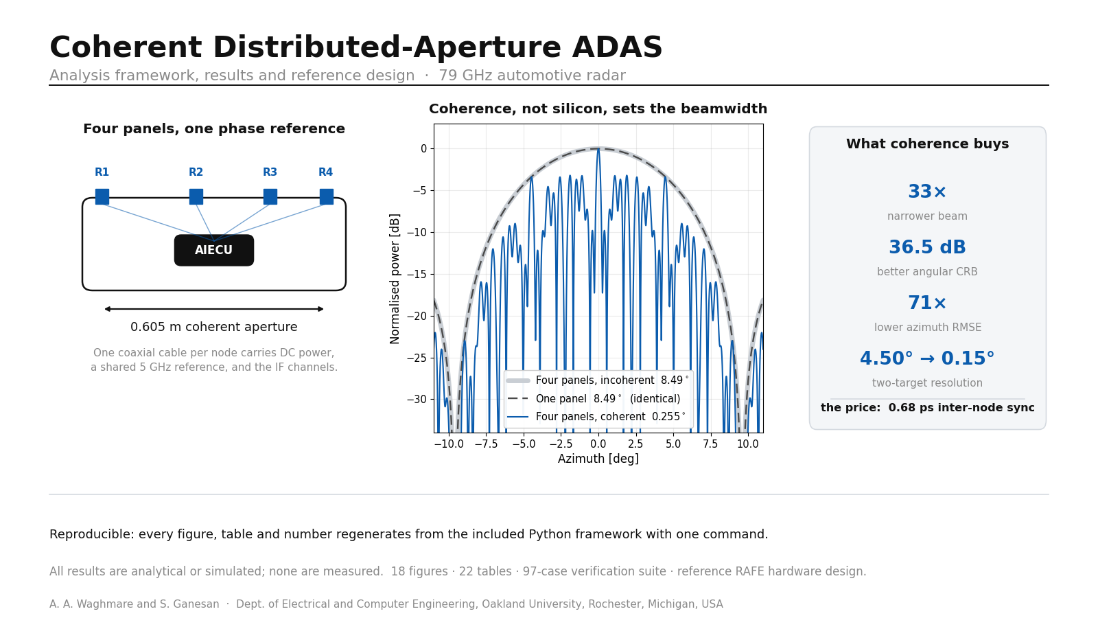
Automotive perception is migrating from self-contained edge sensors toward satellite architectures in which lightly processed data is streamed to a central compute unit. That migration is already underway commercially, and cost reduction is the reason usually given for it. This paper argues that cost is the least interesting consequence of centralisation, and that the decisive one has been largely overlooked: the choice of where to partition the receive chain determines whether the vehicle’s separate radar apertures can be combined phase-coherently into a single synthetic aperture. We define a partition-point taxonomy (P0–P5) for the automotive radar receive chain and show that the two partition points which preserve a shared frequency reference — analogue IF transport (P1) and raw-ADC transport (P2) — enable an aperture whose extent is set by the vehicle, not by the sensor module. We propose an architecture in which each mounting point carries only a Remote Antenna Front-End (RAFE: array, LNA, mixer, frequency multiplier, IF conditioning — no ADC, no DSP, no MCU, no PHY), connected to a unified ADAS Integrated ECU (AIECU) by a single coaxial cable carrying DC power, an up-link frequency reference, and a frequency-division-multiplexed down-link of the IF channels. Quantitatively, for four 3Tx×4Rx panels distributed across a 0.61 m fascia at 79 GHz: the virtual aperture grows from 20.87 mm to 0.605 m, the -3 dB beamwidth narrows from 8.49◦ to 0.255◦, and the Cramér–Rao bound on azimuth improves by 36.5 dB. In single-snapshot Monte Carlo the measured azimuth RMSE at 15 dB SNR improves from 0.203◦ to 0.0028◦, a factor of 71. Two-target resolution at 90 % probability improves from 4.5◦ to 0.15◦. These gains are gated by an unforgiving synchronisation requirement that we quantify: a 0.5 dB coherent-gain budget allows an inter-node RMS carrier-phase error of 0.339 rad, equivalent to 0.68 ps of residual delay or 102 µm of panel displacement at 79 GHz. Timestamp synchronisation cannot approach this — IEEE 802.1AS gPTP at 100 ns corresponds to 4.96 × 10⁴ rad — and neither can an open-loop shared reference, because thermal drift of a 3.5 m coaxial feed at 60 ppm/K over a 145 K automotive range produces 145 ps, or 11.5 whole cycles of carrier phase. We show that closed-loop loopback delay calibration closes the gap, requiring 46 dB of calibration SNR over a 200 MHz sweep against an available link SNR of 96.7 dB. We report a negative result that constrains the design space: the per-node beam is far too broad to disambiguate the coherent aperture. The optimised sparse array’s first grating lobe sits at 1.89◦, while the node beamwidth is 10.42◦, so node-level gating provides no ambiguity protection whatsoever. Ambiguity must instead be managed by co-array-aware panel placement, which reduces the peak sidelobe from -0.20 dB to -3.20 dB and the ambiguity rate at -6 dB SNR from 64.5 % to 21.3 %. At system level, worst-case sensor-to-actuation latency falls from 32.8 ms to 19.6 ms; Monte Carlo over triangular cost distributions gives a mean BOM reduction of 31.8 % against edge sensors (90 % interval $195–$552) and 24.0 % against satellite radar; and a fault-tree analysis shows that the architecture reaches an ASIL-D PMHF of 3.5 × 10⁻⁹/h only when the AIECU is genuinely fail-operational, tolerating a common-cause factor up to β = 0.20.
Keywords: 
;  ;  ;  ;  ;  ;  ;  ;  

1. Introduction

1.1. The Architecture the Industry Is Already Converging on

The module-centric ADAS architecture — in which every radar, camera and ultrasonic sensor is a sealed unit containing RF front-end, ADC, DSP or MCU, memory, power management and a network interface — is being displaced [3]–[5]. Texas Instruments’ AWR2544 is a radar-on-chip designed explicitly for satellite architectures, integrating a 77 GHz 4Tx/4Rx transceiver with a cost-optimised processing accelerator and a 1 Gb/s Ethernet interface for streaming range-FFT-compressed data to a central ECU [1]. Infineon markets the CTRX8191F/CTRX8188F MMICs together with its Carkit platform for integrating raw-ADC satellite radars into centralised ADAS ECUs, citing improved perception, lower node power, unified software lifecycle and cheaper PCB materials [2].
Any paper that proposes “centralised ADAS with lightweight sensor front-ends” as its contribution is therefore proposing a shipping product category. This is worth stating plainly at the outset, because it determines what the actual contribution has to be.

1.2. What Is Genuinely Open

Satellite radar moves processing to the centre. It does not move the frequency reference. Each satellite node still contains a complete MMIC with its own PLL, so the nodes are mutually incoherent by construction. Coherent combination across nodes then becomes an estimation problem — determining the inter-node frequency offset Δf0 and phase offset Δ ϕ from the data itself. A substantial patent family (NXP: US 11092683, US 11269049, US 11520030, US 11888554, US 12235380) [6]–[10] is devoted precisely to this, describing distributed-aperture bistatic MIMO systems that alternate the master transmitter role and apply forward/backward difference co-array processing specifically so as to avoid requiring a shared local oscillator.
The alternative has been demonstrated outside automotive. Photonics-based distributed coherent aperture radar (DCAR) connects a central controller to spatially dispersed remote transceivers over a fibre time-synchronisation network, generating waveforms centrally and performing only optical/RF conversion at the remote heads [12], [13]. In cellular infrastructure the same decomposition is standard: the Cloud-RAN remote radio head with CPRI/eCPRI fronthaul [14], [15].
The open question for automotive is therefore not whether to centralise, but how far down the receive chain to cut, and what that choice does to coherence, harness, latency, dynamic range, safety and cost. That is the question this paper answers.

1.3. The Reframing

We adopt the following thesis:
The value of centralising ADAS processing is not primarily cost. It is that a shared frequency reference converts a set of independent corner sensors into a single vehicle-scale coherent aperture, and the resulting angular resolution is unattainable at any per-node cost.
A 3Tx×4Rx corner radar has a 20.87 mm virtual aperture and an 8.5° beam. No amount of module-level investment changes that: aperture is bounded by the module. Distribute the panels across the fascia under one phase reference and the aperture becomes 0.61 m — a thirty-fold reduction in beamwidth from packaging, not silicon.
This reframing also changes what must be proved. It is no longer enough to assert that centralisation is cheaper. One must show that the coherence is physically attainable in a vehicle, that ambiguity is controllable, that the fronthaul carries the required information, and that concentrating the compute does not violate ISO 26262. Sections VI–IX do this.

1.4. Contributions

1.
A partition-point taxonomy (P0–P5) for the automotive radar receive chain, with quantified fronthaul rate, coherence availability and harness cost at each point (Sec. III, Sec. VII).
2.
The unified sensor cable: a single coax carrying DC power, an up-link frequency reference and a frequency-division-multiplexed down-link of IF channels, which removes the harness penalty that has historically disqualified analogue IF transport (Sec. III-D, Sec. VII-C). We show the link supports 17.0 equivalent bits of SNR and 13.0 bits of spurious-free dynamic range against a 12-bit ADC requirement.
3.
A quantified coherence budget relating array-gain loss to inter-node phase error, residual delay and mechanical displacement, and a demonstration that no timestamp-based synchronisation method can meet it (Sec. VI-A, Sec. VI-B).
4.
A loopback delay-calibration scheme using the same coax, with a closed-form residual-phase expression validated by simulation, plus the observation that the calibration loop doubles as a continuous RF self-test and thereby raises node diagnostic coverage (Sec. VI-D, Sec. IX).
5.
Co-array-aware panel placement as a first-class vehicle design variable, with an optimisation that improves peak sidelobe level by 3.0 dB at fixed aperture and cuts the low-SNR ambiguity rate by a factor of three (Sec. V-C).
6.
A negative result: per-node beam gating cannot disambiguate a vehicle-scale coherent aperture, because the grating-lobe spacing is 5.5× finer than the node beamwidth (Sec. V-E). This closes off an intuitively appealing design path.
7.
A reproducible open analysis framework — signal model, estimators, bounds, coherence models, fronthaul models, cost Monte Carlo and fault tree — with all results in this paper regenerable by a single command (Sec. XIII, Appendix A).

1.5. What We Do Not Claim

We do not claim novelty for centralised ADAS processing, for satellite radar architectures, for distributed aperture radar in general, or for co-array processing. Each has substantial prior art, surveyed in Sec. II. We claim the specific combination of a below-ADC partition point, physical reference distribution over a unified sensor cable, closed-loop delay calibration, and co-array-aware placement — together with the quantitative feasibility envelope that determines whether that combination is buildable.

3. Proposed Architecture

3.1. Partition-point Taxonomy

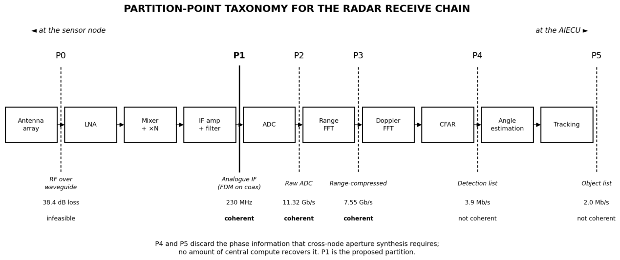
Let the receive chain be: antenna → LNA → mixer → IF filter/amp → ADC → range FFT → Doppler FFT → CFAR → angle estimation → tracking → object list. A partition point is a cut in this chain; everything left of the cut is at the node, everything right is at the AIECU.
Table 2. Partition points in the automotive radar receive chain
Point Node contains Transported Coherence available
P0 Antenna only RF at 79 GHz Yes — but 37.5 dB coax loss over 3.5 m
P1 + LNA, mixer, ×N multiplier, IF amp Analogue IF Yes, structurally
P2 + ADC, serialiser Raw ADC samples Yes, if reference is shared
P3 + range FFT Range-compressed Yes, if reference is shared
P4 + Doppler FFT, CFAR Detection list No
P5 + angle, tracking Object list No
Figure 2. Partition-point taxonomy. The rate collapse between P3 and P4 is three orders of magnitude, and it is exactly where phase coherence is lost.
Preprints 233588 g002
P0 is eliminated by cable physics (Sec. VII-D). P4 and P5 discard the phase information on which cross-node aperture synthesis depends — no amount of central compute can recover it. P1–P3 are the viable region; P1 is the subject of this paper because it removes the most silicon from the node and because it makes reference sharing unavoidable rather than optional.

3.2. The Remote Antenna Front-End (RAFE)

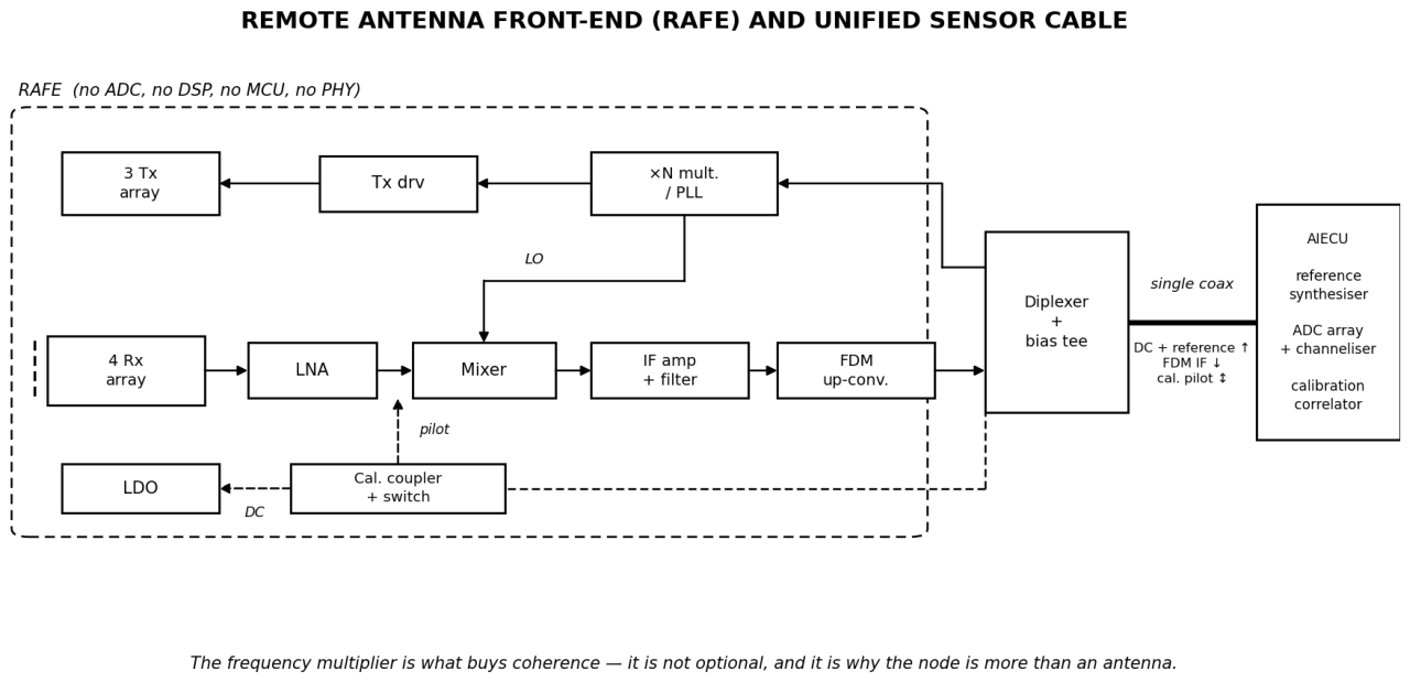
The RAFE contains:
  • a 3Tx × 4Rx patch/waveguide array [4], [26], [27],
  • LNAs and Tx drivers,
  • down-conversion mixers,
  • a frequency multiplier or a small PLL locked to the distributed reference,
  • IF gain and anti-alias filtering,
  • an FDM up-converter (one mixer per Rx channel to its assigned IF slot),
  • a diplexer separating the up-link reference from the down-link IF,
  • a switched directional coupler for loopback calibration,
  • an LDO.
It contains no ADC, no DSP, no MCU, no flash, no Ethernet PHY, no HSM and no local software. This is what distinguishes it from a satellite radar node, and it is what makes the node’s failure rate and diagnostic story materially different (Sec. IX).
It is worth being precise, because the original framing of “just an antenna at each location” overstates it: a frequency multiplier or PLL is still required. That component is what buys coherence, and it is not optional.
Figure 3. RAFE internal block diagram and the unified sensor cable. The receive chain runs left to right; the reference chain runs right to left and supplies the mixer LO.
Preprints 233588 g003

3.3. The AIECU

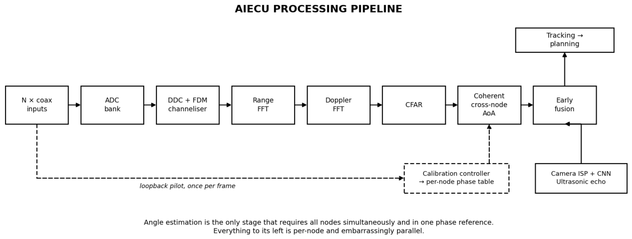
The AIECU performs, for every node simultaneously and in one clock domain: ADC, digital down-conversion and FDM channelisation, range and Doppler FFTs, CFAR, coherent cross-node angle estimation, camera ISP and CNN inference, ultrasonic echo processing, early (cube-level) fusion, tracking, and planning. It hosts the reference synthesiser and the calibration loop.
Its hardware must include a fail-operational compute pair (Sec. IX), a high-channel-count ADC array, and sufficient memory bandwidth for the aggregated data cube.

3.4. The Unified Sensor Cable

This is the element that makes P1 practical. A naive P1 implementation needs one coax per Rx channel — 4 per node, 24 per vehicle — which is a harness regression, not an improvement. The original draft of this work claimed harness simplification while implicitly requiring this explosion; the claim does not survive inspection.
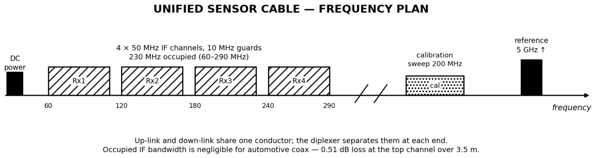
The fix is to treat the cable as a small frequency plan:
  • DC, bias-teed at both ends;
  • up-link: the frequency reference (baseline 5 GHz, premium 19.75 GHz sub-harmonic);
  • down-link: the four Rx IF channels stacked in frequency, 50 MHz each with 10 MHz guards, occupying 60–290 MHz;
  • calibration: a swept pilot returned through the RAFE’s directional coupler.
Total occupied bandwidth is 230 MHz of IF plus a reference tone — still modest for automotive coax, at 1.11 dB of loss. Conductor count drops from 24 (edge or satellite, power pair + data pair per node) to 12.
Figure 4. AIECU processing pipeline. Angle estimation is the only stage requiring all nodes simultaneously in one phase reference; everything to its left is per-node and embarrassingly parallel.
Preprints 233588 g004
Figure 5. Unified sensor cable frequency plan. Up-link and down-link share one conductor; the diplexer separates them at each end.
Preprints 233588 g005
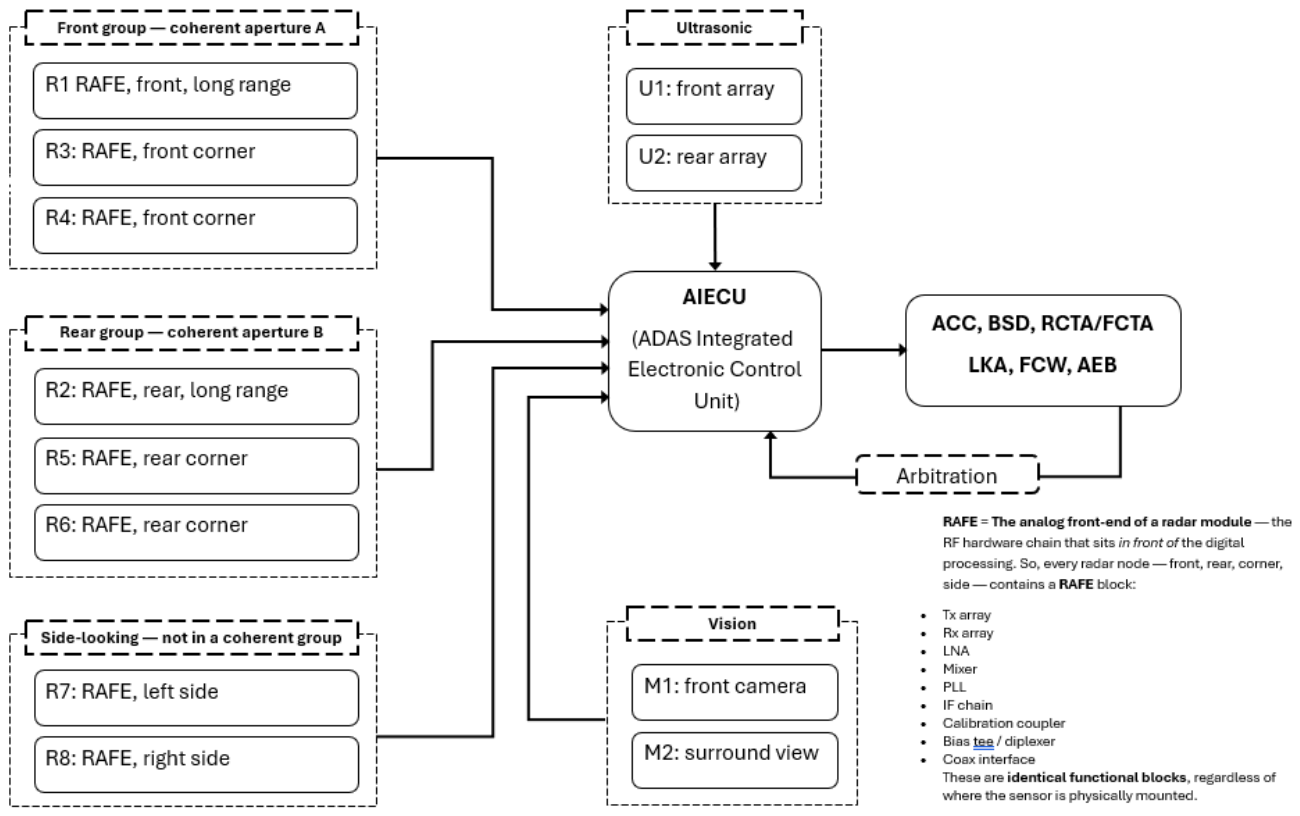
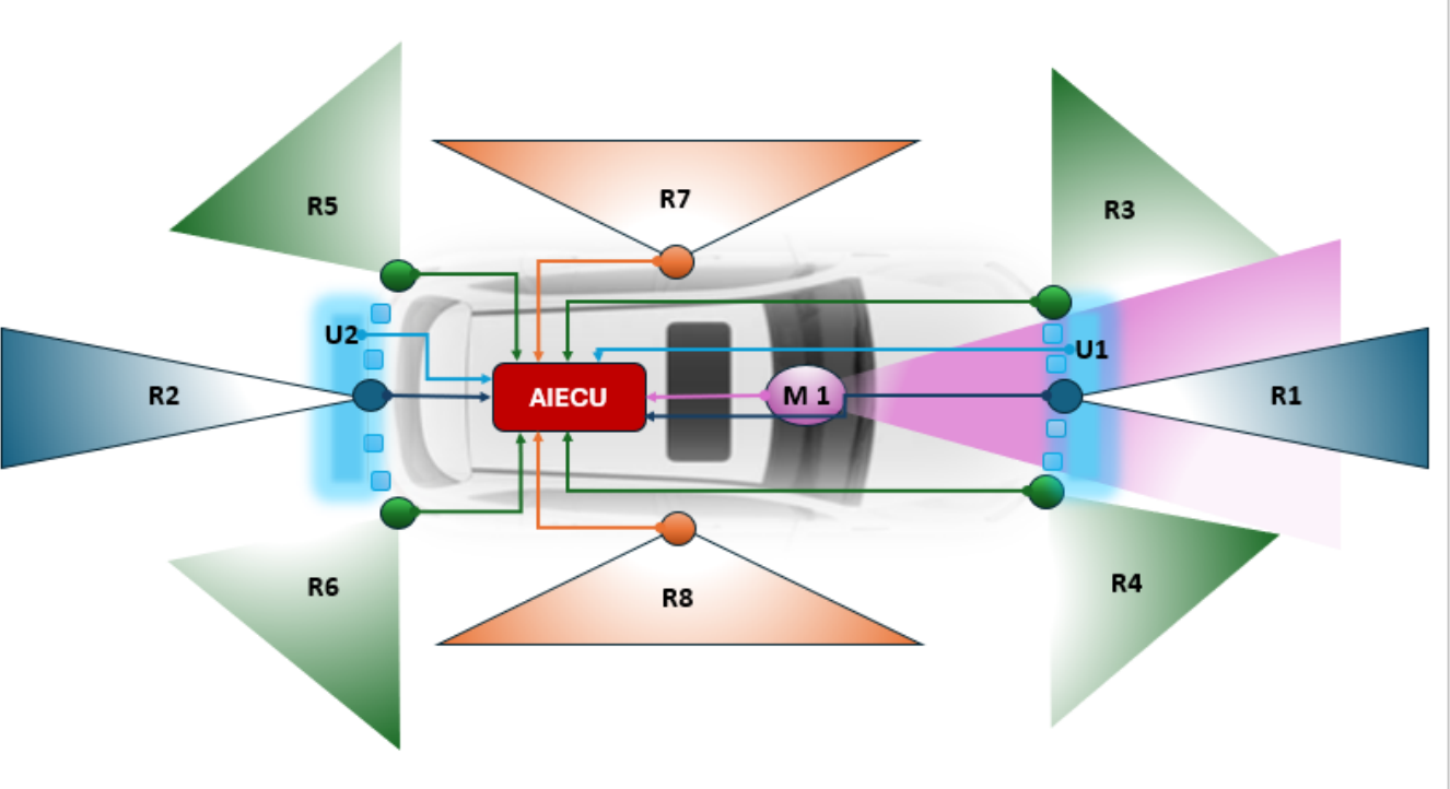
Figure 6. Vehicle sensor set and coverage, vehicle nose to the right. R1 and R2 are the long-range front and rear modules; R3/R4 and R5/R6 are the front and rear corner modules; R7 and R8 look sideways. U1 and U2 are the ultrasonic arrays and M1 the front camera. Every radar node returns analogue IF to the AIECU on one coaxial run.
Preprints 233588 g006

4. Signal Model

4.1. FMCW Beat Signal

For a chirp of slope S = B/Tc, carrier fc, and a point target at range R, radial velocity v and direction cosine u = sin θ , the beat signal at virtual element k with position pk is [20]–[22]
x[n, m, k] = α · exp(j2 π fb n/fs) · exp(j2 π fd m Tc) · exp(j2 π pk u / λ ) · exp(-j2 π fc τ 0)
with fb = S· τ 0, τ 0 = 2R/c and fd = 2v/ λ .

4.2. Virtual Array

For a monostatic MIMO panel the two-way phase for Tx at xt and Rx at xr depends on (xt + xr)·u, so the virtual element positions are the Minkowski sum of the Tx and Rx sets [23], [24]. With Tx spacing 4·( λ /2) and Rx spacing λ /2, a 3×4 panel yields a filled 12-element ULA at λ /2 spanning 20.87 mm.
Concatenating N panels at fascia offsets {oi} gives a sparse array of 12N elements. The steering vector is a(u)k = exp(j2 π pk u/ λ ).

4.3. Impairments

Per-node impairments enter as a common factor on all elements of that panel:
xk∈node i = xk · exp(j ϕ i) · exp(j2 π fc Δ τ i) · exp(j2 π Δ fi m Tc) · exp(j2 π S Δ τ i n/fs)
The second factor is the one that matters. Because it is multiplied by fc, not by the IF bandwidth, a delay error that is negligible for range estimation is catastrophic for angle estimation. Sec. VI quantifies this.
The Δfi term exists only for independent-LO architectures. In the proposed architecture it is identically zero — the nodes cannot drift relative to one another in frequency because they are all multiplications of the same reference. This is the structural difference from satellite radar.

4.4. Implementation

@dataclass
class RAFEGeometry:
    n_tx: int = 3
    n_rx: int = 4
    fc: float = 79.0e9
    offset: float = 0.0
    @property
    def virtual_positions(self) -> np.ndarray:
        v = (self.tx_positions[:, None] + self.rx_positions[None, :]).ravel()
        return np.sort(v) + self.offset
# per-node impairments broadcast to elements, then applied to the cube
spat = np.exp(1j * 2 * np.pi * positions * tgt.u / cfg.lam)
spat = spat * np.exp(1j * (ph_el + 2 * np.pi * cfg.fc * dt_el))

5. The Coherent Distributed Aperture

5.1. Aperture and Resolution

Four panels on a 0.61 m fascia:
Table 3. Aperture and resolution, single panel versus coherent four-panel array
Quantity Single panel Coherent 4-panel
Virtual elements 12 48
Aperture 20.87 mm 0.605 m
-3 dB beamwidth 8.494° 0.255°
Peak sidelobe level -13.06 dB -3.20 dB
CRB σ θ at 10 dB SNR 0.0853° 0.00127°
The resolution gain is 33.4× and the accuracy gain 36.5 dB. The sidelobe degradation from -13 dB to -3.2 dB is the price of sparsity and is the subject of Sec. V-C and Sec. V-E.
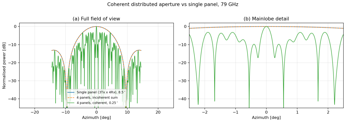
Figure 7. Beampattern of a single panel, four panels summed incoherently, and four panels combined coherently. The incoherent sum has the same beamwidth as one panel; only coherent combination narrows the mainlobe.
Preprints 233588 g007

5.2. Cram ér–Rao Bound

We use the exact deterministic single-source bound [25], [33], [36],
CRB(u) = σ 2 / (2 L | α |2∥Pa⊥∂a/∂u∥2),
computed numerically from the steering-vector derivative rather than from a closed-form aperture approximation, so it remains exact for sparse geometries.
def crb_u(positions, u0, lam, snr_db, n_snap):
    a = steering(positions, u0, lam)[:, 0]
    da = (1j * 2.0 * np.pi * positions / lam) * a
    P = np.eye(a.size) - np.outer(a, a.conj()) / (a.conj() @ a).real
    num = np.linalg.norm(P @ da) ** 2
    return 1.0 / (2.0 * n_snap * 10 ** (snr_db / 10.0) * num)

5.3. Co-array-aware Panel Placement

Panel positions on the fascia are a design variable, not a given; the relevant theory is that of minimum-redundancy, nested and coprime arrays [28]–[30]. At fixed aperture (0.605 m) and fixed panel count:
Table 4. Effect of panel placement at fixed aperture
Placement Offsets ( λ /2 units) PSL -3 dB BW
Uniform 0, 103, 206, 308 -0.20 dB 0.255°
Hand-picked sparse ruler 0, 57, 149, 308 -1.67 dB 0.253°
Optimised 0, 129, 231, 308 -3.20 dB 0.255°
Table 5. Two-target resolution at 90,% probability
Estimator Separation at P(resolve) = 0.9
Single panel 4.50°
Coherent aperture 0.15°
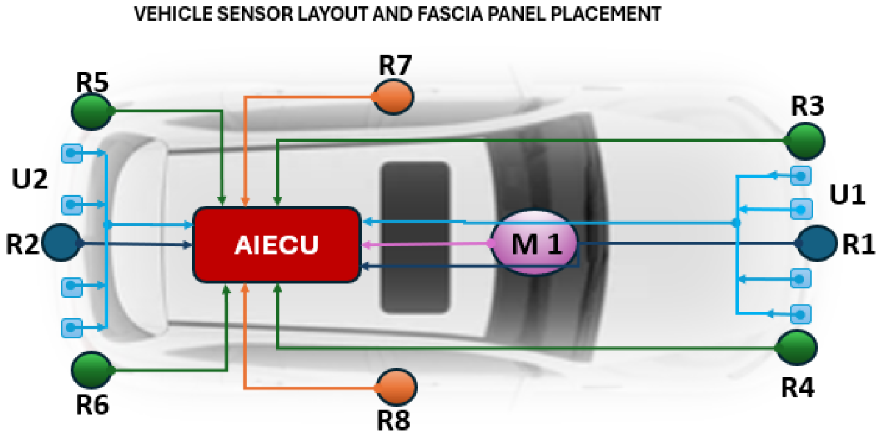
Figure 8. Front fascia panel placement, vehicle nose upward. Offsets 0 / 129 / 231 / 308 half-wavelengths (0 / 24.5 / 43.8 / 58.4 cm) are a sidelobe optimisation, not a packaging accident: uniform spacing at the same aperture leaves a -0.20 dB grating lobe, while this placement reaches -3.20 dB.
Preprints 233588 g008
Uniform spacing is nearly pathological: a -0.20 dB grating lobe is essentially a second mainlobe. Random search over interior offsets improves this by 3.0 dB at no cost in aperture or hardware. The difference co-array remains holey (longest contiguous run 11 lags out of 319 with four panels), so this is sidelobe management rather than co-array completion; hole-free co-arrays at this aperture would require substantially more panels.

5.4. Estimation and Resolution Performance
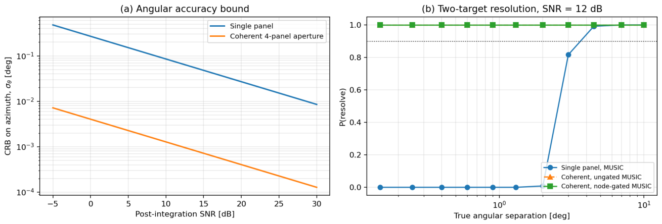
Two-target resolution probability, MUSIC [31] — with ESPRIT [32], Capon [34] and conventional beamforming [35] as the standard alternatives — at 12 dB SNR:
Figure 9. (a) CRB on azimuth versus SNR. (b) Two-target resolution probability versus separation.
Preprints 233588 g009
Table 6. Grating-lobe spacing against the node beamwidth
Quantity Value
Node beamwidth 10.42°
First grating lobe, uniform placement 1.11°
First grating lobe, optimised placement 1.89°

5.5. Negative Result: Node-Beam Gating Does Not Work
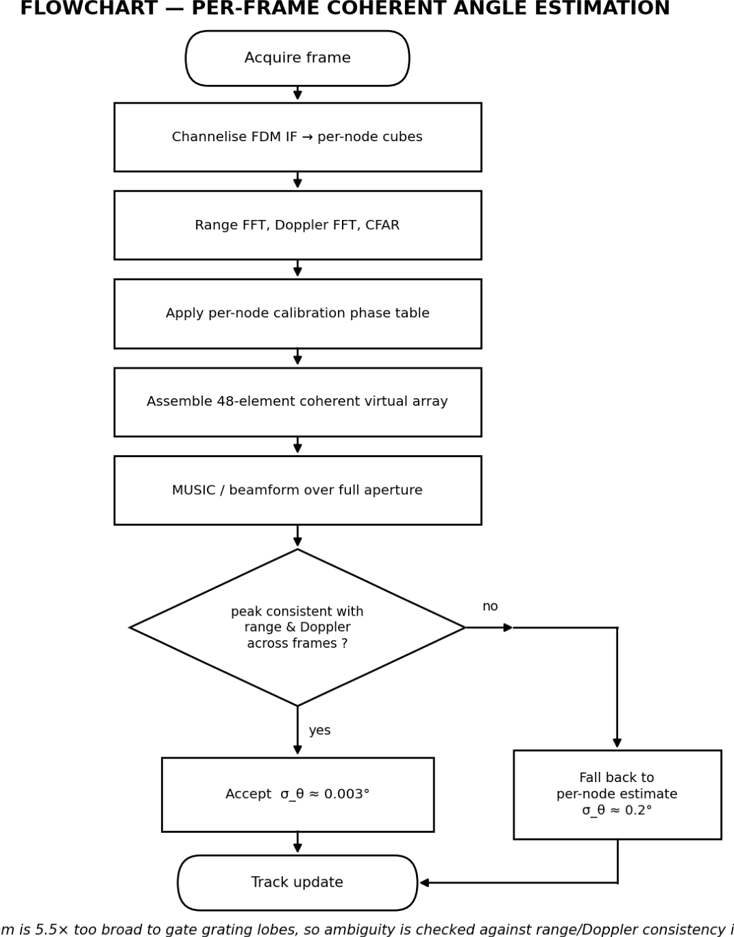
A natural design instinct is to use the unambiguous per-node beam as a gate on the ambiguous coherent spectrum — a coarse-to-fine estimator. We implemented this and it does not help, for a structural reason:
Figure 10. Per-frame coherent angle estimation. Because the node beam cannot gate grating lobes, ambiguity is checked against range and Doppler consistency across frames instead.
Preprints 233588 g010
The grating lobes are 5.5× finer than the gate. Dozens of them fall inside the node beam, so the gate admits all of them. We report this because the intuition is appealing and, we suspect, common; it should be closed off explicitly rather than left for others to rediscover. Ambiguity control at vehicle scale must come from placement design, Doppler and range consistency across frames, or genuine co-array completion — not from the node pattern.
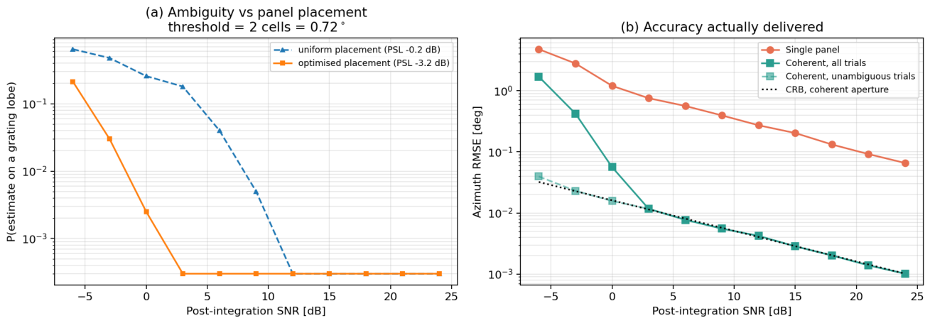
An earlier version of this analysis scored ambiguity against half a node beamwidth and consequently reported ~0 % ambiguity everywhere. That threshold was wrong: it classified grating-lobe locks as successes. Scored correctly, against two coherent resolution cells (0.718°):
Table 7. Grating-lobe ambiguity rate versus placement and SNR
SNR Ambiguity rate, uniform Ambiguity rate, optimised
-6 dB 64.5 % 21.3 %
-3 dB 47.8 % 3.0 %
0 dB 25.8 % 0.25 %
≥ 6 dB ≤ 4 % 0 %
Placement optimisation buys roughly a 9 dB shift in the SNR at which ambiguity collapses.

5.6. Net Delivered Accuracy

Single-snapshot Monte Carlo, conventional beamforming, outliers included:
Table 8. Delivered azimuth RMSE, single snapshot, outliers included
SNR Single panel RMSE Coherent RMSE (all trials)
0 dB 1.201° 0.056°
6 dB 0.563° 0.0077°
15 dB 0.203° 0.0028°
24 dB 0.066° 0.0010°
At 15 dB the delivered gain is 71×, with zero ambiguous trials.
Figure 11. (a) Grating-lobe ambiguity rate versus SNR for uniform and optimised placement, scored against two coherent resolution cells. (b) Azimuth RMSE actually delivered, outliers included.
Preprints 233588 g011

6. The Coherence Budget

This section contains the result that determines whether the architecture is buildable.

6.1. Allowance

For i.i.d. zero-mean Gaussian element phase errors, the coherent sum is attenuated by the characteristic function exp(- σ ϕ 2/2), so power loss is exp(- σ ϕ 2).
Table 9. Inter-node phase-error allowance
Gain loss σ ϕ Equivalent delay at 79 GHz Equivalent displacement
0.2 dB 0.215 rad (12.3°) 0.432 ps 64.8 μ m
0.5 dB 0.339 rad (19.4°) 0.684 ps 102 μ m
1.0 dB 0.480 rad (27.5°) 0.967 ps 145 μ m
3.0 dB 0.831 rad (47.6°) 1.674 ps 251 μ m
The mechanical column is a genuine constraint: 102 μ m of bumper flex is within the range of thermal expansion and road load, so panel mounting stiffness becomes an RF specification.

6.2. Why Timestamp Synchronisation Cannot Work

Table 10. Synchronisation methods against the 0.5,dB coherence budget
Method Residual delay Carrier phase at 79 GHz Meets 0.5 dB?
IEEE 802.1AS gPTP, typical 100 ns 4.96 × 10⁴ rad No
IEEE 802.1AS gPTP, best case 10 ns 4.96 × 10³ rad No
White Rabbit / sub-ns PTP 100 ps 49.6 rad No
Shared reference, uncalibrated coax 60 ps 29.8 rad No
Shared reference + loopback calibration 0.4 ps 0.200 rad Yes
Even sub-nanosecond network synchronisation — far beyond what any production vehicle deploys — misses by two orders of magnitude. This is the central reason coherence cannot be retrofitted onto a satellite architecture by improving its network timing. It is a physical-layer problem.

6.3. Why Open-Loop Reference Distribution Also Fails

A 3.5 m coaxial feed has ≈16.7 ns one-way delay. At a delay temperature coefficient of 60 ppm/K over the -40 °C to +105 °C automotive range:
  • delay drift: 145 ps
  • carrier phase drift: 72.0 rad = 11.5 whole cycles
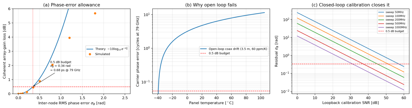
Distributing a reference is necessary but not sufficient. Without a calibration loop the architecture fails on the first cold morning.
Figure 12. (a) Array-gain loss versus inter-node phase error, theory and simulation. (b) Open-loop coaxial drift against the 0.5 dB budget. (c) Residual phase after closed-loop loopback calibration.
Preprints 233588 g012

6.4. Loopback Delay Calibration

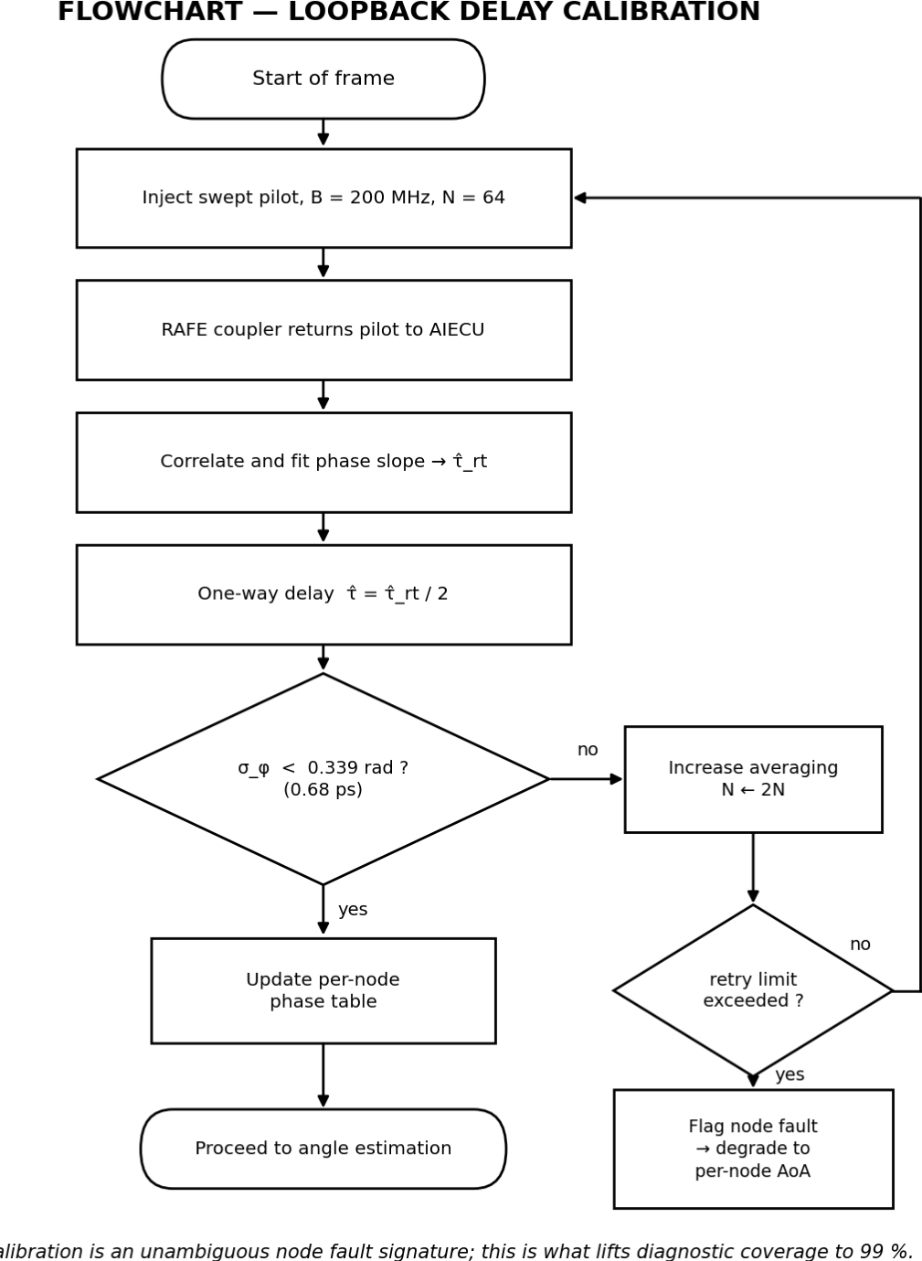
The scheme is the wired analogue of round-trip carrier synchronisation in distributed transmit beamforming [39], [40]. The AIECU sweeps a pilot tone up the coax; a switched directional coupler at the RAFE returns it; the AIECU fits the phase slope to estimate the round-trip delay, halving it for the one-way value. For a linear-phase fit over N tones spanning B:
var( τ rt) = 3 / (2 π 2· SNR · N · B2)
def loopback_residual_phase_rad(snr_db, bw_hz, n_avg=64, fc=79.0e9):
    snr = 10.0 ** (snr_db / 10.0)
    var_tau_rt = 3.0 / (2.0 * np.pi ** 2 * snr * n_avg * bw_hz ** 2)
    sigma_tau = np.sqrt(var_tau_rt) / 2.0
    return 2.0 * np.pi * fc * sigma_tau
With a 200 MHz sweep and 64 averages, meeting the 0.339 rad budget requires 46 dB of calibration SNR. The IF link provides 96.7 dB (Sec. VII-C). The margin is 51 dB. With a 1 GHz sweep the requirement drops to roughly 32 dB.
The loop is not free: it consumes a small fraction of the frame time and requires a coupler and switch at each node. It also, usefully, constitutes a continuous end-to-end RF self-test — a failed calibration is an unambiguous node fault indication. Sec. IX credits this in the diagnostic coverage.
Figure 13. Loopback delay calibration. A failed calibration is an unambiguous node fault signature, which is what lifts node diagnostic coverage to 99 % in Sec. IX.
Preprints 233588 g013

6.5. Residual PLL Phase Noise

Below the node PLL’s loop bandwidth the nodes track the shared reference and their phase noise is common-mode [37], cancelling in inter-node differences. Only the uncorrelated region above the loop bandwidth contributes. Integrating a -88 dBc/Hz at 1 MHz mask with -20 dB/decade slope:
Phase noise is a second-order term. Delay calibration dominates the budget. The range-correlation effect [38] further suppresses close-in noise for the short ranges typical of corner sensing.
Table 11. Residual phase noise of the node PLL above loop bandwidth
Loop bandwidth σ ϕ Gain loss
0.3 MHz 0.103 rad 0.046 dB
1 MHz 0.056 rad 0.014 dB
3 MHz 0.032 rad 0.004 dB

6.6. End-to-end Degradation

Table 12. End-to-end degradation versus residual inter-node phase error
σ ϕ Measured gain loss Theory Azimuth RMSE
0.00 0.00 dB 0.00 dB 0.0014°
0.10 0.03 dB 0.04 dB 0.0076°
0.20 0.13 dB 0.17 dB 0.017°
0.35 0.46 dB 0.53 dB 0.319°
0.50 0.90 dB 1.09 dB 0.718°
0.80 2.05 dB 2.78 dB 0.988°
1.20 3.95 dB 6.25 dB 1.108°
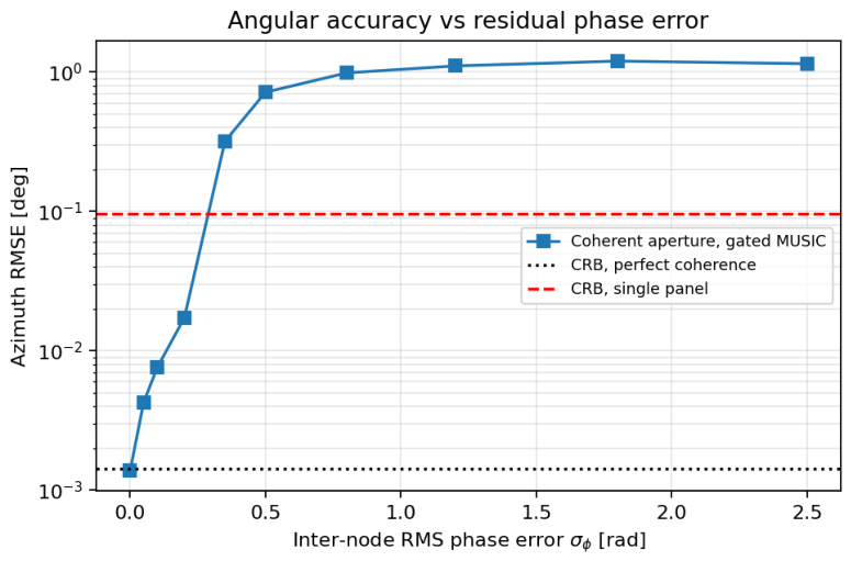
Two observations. First, theory and measurement agree closely for σ ϕ ≲ 0.35 and diverge above it — the theoretical expression describes the mean coherent sum, whereas the measured value is the peak of a partially randomised pattern, which is bounded below by the incoherent floor. The theory is therefore conservative in exactly the region where it matters and pessimistic elsewhere.
Second, and more important for system design: RMSE degrades far faster than array gain. At σ ϕ = 0.35 the gain loss is a tolerable 0.46 dB, but RMSE has already risen 230× from its coherent value to 0.319° — because phase errors do not merely attenuate the mainlobe, they raise sidelobes into ambiguity territory. The synchronisation specification must be set by angular accuracy, not by array gain. A budget derived from a gain-loss allowance alone would be dangerously loose.
Figure 14. Azimuth RMSE versus residual inter-node phase error, against the coherent and single-panel bounds.
Preprints 233588 g014

7. Fronthaul

7.1. Rate by Partition Point

Per node: 4 Rx × 3 Tx, 2560 fast-time samples, 128 chirps, 20 frames/s, 12-bit ADC.
Table 13. Fronthaul rate by partition point
Partition Per node Per vehicle (6 nodes) Coherence
P1 analogue IF (FDM) 230 MHz occupied analogue Yes
P2 raw ADC 1887 Mb/s 11.32 Gb/s Yes
P3 range FFT 1258 Mb/s 7.55 Gb/s Yes
P4 detection list 0.66 Mb/s 3.9 Mb/s No
P5 object list 0.33 Mb/s 2.0 Mb/s No
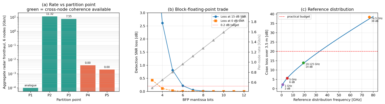
The rate collapse between P3 and P4 is three orders of magnitude — and it is exactly where coherence is lost. This is the central trade of the architecture, and it is why “reduce the fronthaul” and “improve the perception” are in direct tension in every digital partition scheme.
Figure 15. (a) Aggregate fronthaul by partition point; green indicates cross-node coherence remains available. (b) Block-floating-point compression trade. (c) Coaxial loss versus reference distribution frequency.
Preprints 233588 g015

7.2. Compression at P2/P3

Block floating point with a shared exponent per 32-sample block [42]:
Table 14. Block-floating-point compression trade at P2/P3
Mantissa bits Ratio SQNR Loss at 15 dB SNR Per-node rate
5 2.34 21.9 dB 0.814 dB 806 Mb/s
6 1.96 27.9 dB 0.218 dB 963 Mb/s
7 1.68 33.9 dB 0.056 dB 1121 Mb/s
8 1.48 39.9 dB 0.014 dB 1278 Mb/s
Seven mantissa bits is the first setting to clear a 0.2 dB detection-loss target (six bits misses it marginally at 0.218 dB). Note that compression is a digital-partition concern; P1 does not have it, which is one of the simplifications the analogue partition buys.

7.3. IF-FDM Link Budget

Four channels, 50 MHz each, 10 MHz guards, 3.5 m coax:
The link is not noise-limited; it is intermodulation-limited. At the 79 GHz band’s full 4 GHz sweep this margin has become thin: 75.2 dB of SFDR is 12.2 equivalent bits against a 12-bit ADC requirement, where the 1 GHz configuration had 13.0. Linearity, not loss, is therefore the binding constraint on how many IF channels may share one coax. Raising the IF amplifier to OIP3 = +27 dBm restores 13 bits of SFDR; alternatively the four channels can be split across two coaxial runs per node, at the cost of the harness advantage in Sec. VII-E. Cable loss at IF is negligible and, critically, follows the node’s 25 dB IF gain, so its noise-figure contribution is second-order.
This is the quantitative answer to the standard objection that analogue transport is fragile: over 3.5 m at 66 MHz, it is not.
Table 15. Analogue IF frequency-division-multiplex link budget
Quantity Value
Occupied bandwidth 230 MHz (60–290 MHz)
Coax loss at top channel 1.11 dB
Received power +3.89 dBm
Noise floor -92.8 dBm
Link SNR 96.7 dB (15.8 ENOB)
SFDR (OIP3 = +20 dBm) 75.2 dB (12.2 bits)

7.4. Reference Distribution

Table 16. Reference-distribution options over 3.5,m of coaxial cable
Scheme Frequency Loss over 3.5 m Verdict
Direct LO 79 GHz 37.5 dB Infeasible
Sub-harmonic, ×4 at node 19.75 GHz 13.9 dB Feasible with driver amp
Reference + node PLL 5 GHz 5.65 dB Baseline
Reference + node PLL 1 GHz 2.19 dB Lowest loss, highest multiplication noise
The loss model includes both skin-effect (∝ . f) and dielectric (∝f) terms [41]. A . f-only model — which we used initially — underpredicts 79 GHz loss by more than a factor of two and would have made direct LO distribution look merely difficult rather than impossible.
Multiplying a 5 GHz reference to 79 GHz costs 20·log10(15.3) = 23.7 dB of phase-noise multiplication, which Sec. VI-E shows is affordable.

7.5. Harness

Table 17. Harness comparison, six radar nodes
Architecture Cables/node Conductors/node Total conductors (6 nodes)
Edge sensor 1 4 24
Satellite radar 1 4 24
Naive IF-per-channel 4 8 48
Proposed IF-FDM 1 2 12
The naive row is the one the original draft implicitly proposed. FDM turns a 2× harness regression into a 2× improvement.

8. Latency

Table 18. End-to-end sensor-to-actuation latency
Architecture Typical Worst case Reaction distance at 120 km/h
Edge sensors 17.3 ms 32.8 ms 1.09 m
Satellite radar 13.5 ms 23.4 ms 0.78 m
Proposed 11.95 ms 19.55 ms 0.65 m
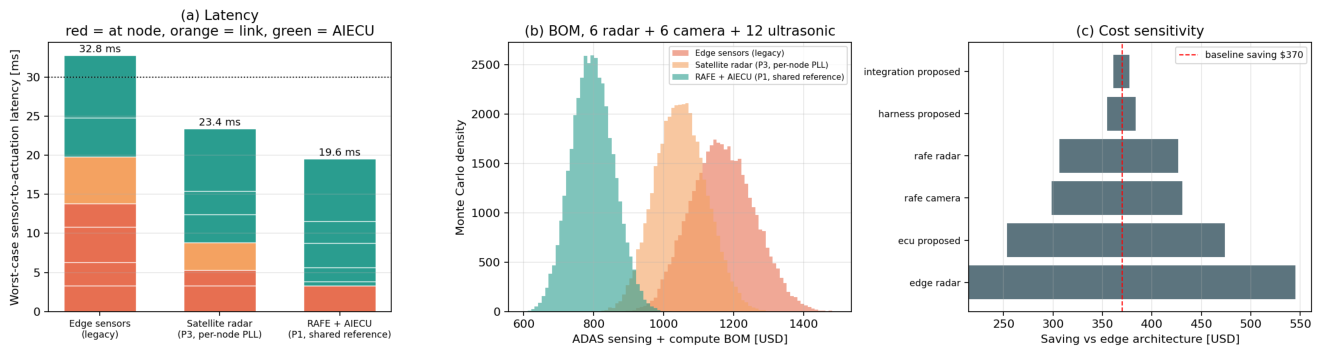
The reduction comes from eliminating node-side processing stages and their queueing, not from the link: analogue IF propagation over 3.5 m is 20 ns, six orders of magnitude below the frame time. Frame acquisition (3.3 ms) and planning (up to 8 ms) dominate all three architectures, which bounds how much any fronthaul change can achieve — a point the original draft’s “<10 ms end-to-end” target did not account for. That target is not reachable while a 128-chirp frame takes 3.3 ms to acquire and planning takes 4–8 ms; 19.6 ms worst case is the honest figure.
Figure 16. (a) Worst-case latency by stage and location. (b) BOM Monte Carlo. (c) Cost sensitivity.
Preprints 233588 g016

9. Functional Safety

Centralisation’s strongest objection is that it concentrates failure. The answer is not “make it ASIL-D” [45] — that is a requirement, not a design — but a quantified fault tree.
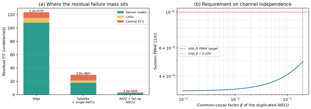
Residual (undetected) FIT, 6 nodes:
Table 19. Residual failure rate and PMHF by architecture
Architecture Nodes Links ECU Total PMHF ASIL-D
Edge + fusion ECU 108.0 7.2 8.5 123.7 1.24 × 10⁻⁷/h No
Satellite + single AIECU 17.7 3.6 8.5 29.8 2.98 × 10⁻⁸/h No
RAFE + fail-operational AIECU 2.52 0.72 0.26 3.50 3.50 × 10⁻⁹/h Yes
Two effects drive this, and both deserve scrutiny.
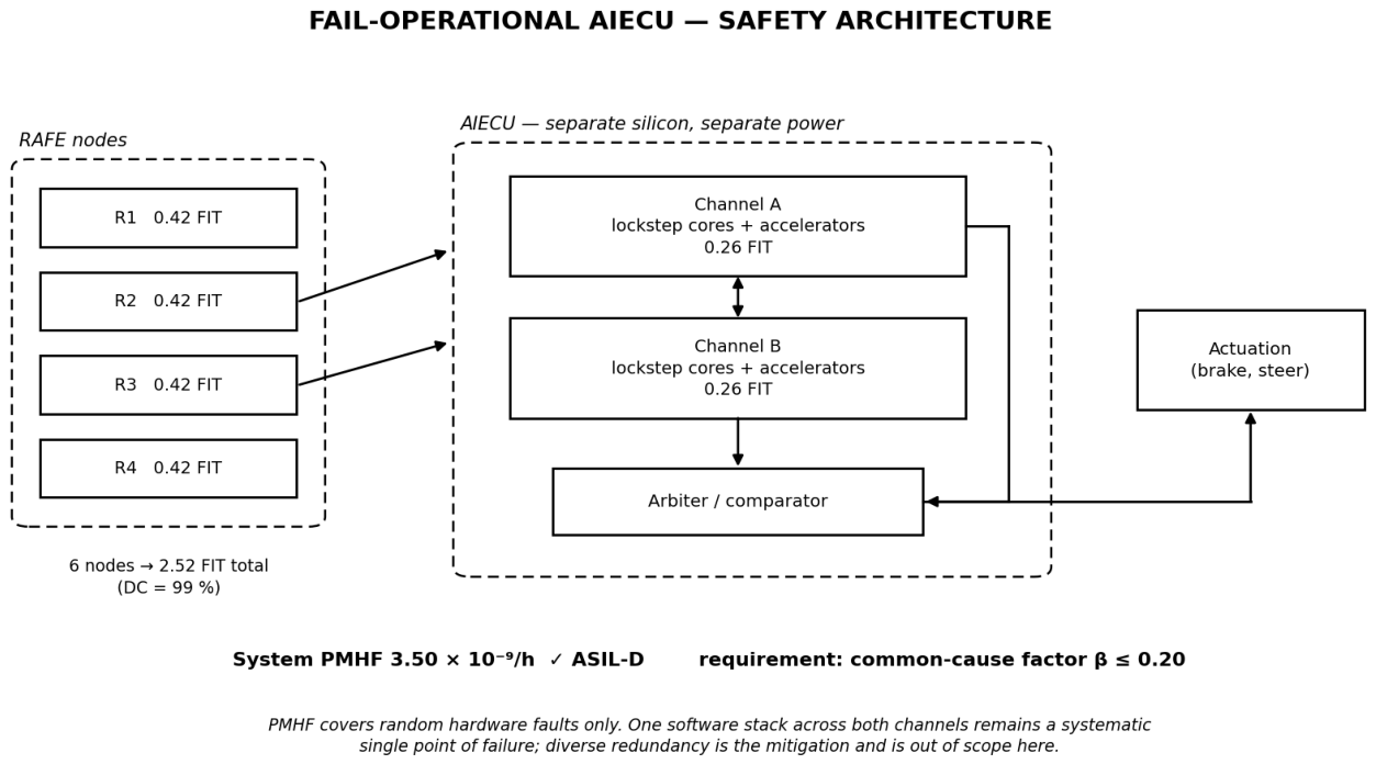
Figure 17. Fail-operational AIECU. Channel A reports to the arbiter around channel B, not through it, so a channel fault cannot mask itself.
Preprints 233588 g017
Node simplification. Removing the ADC, DSP, MCU, flash and PHY takes the node from 180 FIT to 42 FIT. This is a straightforward consequence of component count.
Diagnostic coverage. We assign 90 % coverage to edge nodes, 95 % to satellite nodes and 99 % to RAFEs. The last is the load-bearing assumption and it needs justification: the AIECU sees raw data from every node in a common phase reference, so it can run cross-node plausibility tests that no edge sensor can run on itself, and the loopback calibration loop (Sec. VI-D) is a continuous end-to-end RF integrity check whose failure is unambiguous. A degradation in inter-node coherence is itself a fault signature. If a reviewer rejects the 99 % figure, the conclusion weakens proportionally — at 95 % coverage the proposed architecture yields 13.6 FIT and still passes, at 90 % it yields 26.5 FIT and still passes, so the conclusion is robust even though the headline number is not.
Fail-operational requirement. The single-AIECU rows fail. Duplication with common-cause factor β = 0.03 brings the ECU contribution from 8.5 FIT to 0.26 FIT. Sweeping β shows ASIL-D is met for β ≤ 0.20, which is a comfortable requirement — achievable with separate silicon, separate power domains and separate physical placement, though not with two cores on one die.
Figure 18. (a) Residual failure mass by architecture. (b) PMHF versus common-cause factor of the duplicated AIECU.
Preprints 233588 g018
A residual concern the model does not capture: centralisation creates a single point of systematic failure — one software stack, one supplier, one vulnerability. PMHF addresses random hardware faults only. Diverse redundancy in the fail-operational channel is a plausible mitigation and is out of scope here.

10. Cost

Monte Carlo over triangular distributions, 40 000 draws, for 6 radar + 6 camera + 12 ultrasonic positions.
Table 20. Bill-of-materials Monte Carlo, sensing and compute
Architecture Mean P5 P50 P95
Edge sensors $1168 $1022 $1166 $1320
Satellite radar $1048 $930 $1047 $1172
Proposed $796 $700 $795 $898
Table 21. Cost saving of the proposed architecture
Comparison Mean saving 90 % interval P(saving > 0)
vs edge $371 (31.8 %) $195 – $552 99.99 %
vs satellite $252 (24.0 %) $96 – $409 99.7 %
The original draft asserted “20–30 % reduction” without derivation. The interval above happens to contain that range, but the interval is the result; the point estimate alone is not defensible. Sensitivity analysis ranks the drivers by swing, in order: edge radar unit cost (the baseline being displaced), AIECU cost, RAFE camera cost, RAFE radar cost, harness, integration. The first entry is worth reading carefully — the largest single determinant of the saving is not how cheap the RAFE is but how expensive the incumbent edge radar is, which means the case weakens as edge-sensor prices fall. The AIECU is the only driver that moves against the architecture, and even at its maximum the mean saving remains positive.
Two costs the model omits and a reviewer will ask about: NRE for a new node/ECU interface and the ecosystem cost of departing from standard SerDes/Ethernet transport. Both are real and both favour satellite radar in the near term.

11. Discussion and Limitations

Simulation, not measurement. Every result here is analytical or simulated. The coherence budget in particular assumes a delay-drift model and a calibration SNR; a bench measurement on 3.5 m of automotive coax across the temperature range is the necessary next step and could invalidate Sec. VI-C in either direction.
Four panels is few. The difference co-array cannot be completed with four panels at 0.63 m aperture, which is why sidelobes remain at -3.2 dB. Six or eight panels would allow genuine co-array design and would likely remove the ambiguity concern entirely. We chose four because it matches plausible front-fascia mounting.
Single-target and two-target scenes only. Dense clutter, extended targets, multipath and interference from other vehicles’ radars are not modelled. Mutual interference is a particular concern [43], [44]: a coherent aperture is also a coherent interference aperture.
Camera and ultrasonic claims are weaker than the radar claims. There is no coherence argument for cameras — centralising the ISP is a real benefit (unified tuning, cheaper modules, early fusion on raw Bayer data) but it is an engineering convenience, not a physics gain. Ultrasonic raw echo transport is bandwidth-trivial and the benefit is mostly BOM. The original draft treated all three modalities as equivalent beneficiaries of centralisation; they are not, and the paper is stronger for saying so.
Thermal. Concentrating all DSP and inference into one enclosure creates a thermal problem the original draft noted but did not quantify. We have not quantified it either; it is a genuine gap.
Regulatory and EMC. Radiating IF on a coax through a vehicle harness has EMC implications not addressed here.

12. Roadmap

1.
Bench validation of the coherence budget — two RAFE prototypes, one reference, one calibration loop, measured phase stability over -40 °C to +105 °C. This single experiment determines whether the architecture is viable.
2.
Anechoic characterisation of the 4-panel array: measured beampattern against Fig. 7, measured two-target resolution against Fig. 9.
3.
Vehicle integration with mounting stiffness characterised against the 102 μ m displacement budget.
4.
Interference study in a multi-radar environment.
5.
Standardisation of the unified sensor cable frequency plan, which is the natural point of ecosystem contention.

13. Conclusions

Centralised ADAS is not a proposal; it is the direction the industry is already taking, and cost is the reason usually given. We have argued that cost is the wrong headline. The partition point in the radar receive chain determines whether the vehicle’s apertures can be combined coherently, and coherence is worth 33× in beamwidth, 36.5 dB in angular CRB and 71× in delivered azimuth RMSE — a capability unattainable at any per-node price, because aperture is bounded by packaging.
The price of that capability is a synchronisation requirement of 0.68 ps, which no timestamp-based method can approach and no open-loop reference distribution can hold across temperature. Closed-loop loopback calibration over the same coax that carries power, reference and IF closes the gap with 59 dB of margin, and the calibration loop pays for itself again as a continuous diagnostic that lifts node coverage enough to reach an ASIL-D PMHF of 3.5 × 10⁻⁹/h — provided the AIECU is genuinely fail-operational.
We also report what does not work: the per-node beam is 5.5× too broad to disambiguate a vehicle-scale aperture, so ambiguity must be handled by placement design, where a 3.0 dB sidelobe improvement is available for free.
The architecture is buildable if and only if the picosecond-scale coherence budget survives contact with a real vehicle harness. That is a bench experiment, not an argument, and it is the next thing to do.

Appendix A. Reproducibility

aiecu/
  aiecu/
    geometry.py    virtual arrays, difference co-array
    fmcw.py        FMCW cube and snapshot models
    dsp.py         Bartlett, MUSIC, co-array, CRB, CFAR
    sync.py        coherence budget, drift, calibration
    fronthaul.py   partition rates, BFP, link budget
    system.py      latency, BOM Monte Carlo, fault tree
  experiments/
    exp1_aperture.py    beampattern, CRB, resolution
    exp1b_ambiguity.py  grating-lobe analysis
    exp2_coherence.py   budget, drift, calibration
    exp3_fronthaul.py   rates, compression, link budget
    exp4_system.py      latency, cost, safety
    exp5_diagrams.py    block diagrams and flowcharts
    build_ieee.py       IEEEtran two-column LaTeX + PDF
    build_docx.py       IEEE-styled two-column Word
    run_all.py
  figures/    17 result figures and diagrams
  results/    JSON for every number in this paper
pip install -r requirements.txt
python experiments/run_all.py
Every table entry in Sec. V–Sec. X is read from results/*.json. Random seeds are fixed per experiment.

Appendix B. Key Parameters

Table A1. Key system parameters
Parameter Value
Carrier 79 GHz ( λ = 3.795 mm)
Sweep bandwidth 4 GHz (range resolution 3.75 cm)
Chirp duration 25.6 μ s, 128 chirps (frame 3.28 ms)
IF sample rate 100 MHz, 2560 samples
Panel 3 Tx × 4 Rx → 12-element virtual ULA, 20.87 mm
Array 4 panels, offsets 0/129/231/308 ( λ /2), aperture 0.605 m
Fronthaul 1 coax/node: DC + 5 GHz reference up, 60–290 MHz IF FDM down
Coherence budget σ ϕ ≤ 0.339 rad (0.68 ps, 102 μ m) for 0.5 dB

References

  1. Texas Instruments. “AWR2544 single-chip 76–81 GHz FMCW radar sensor for satellite architectures,” Product Datasheet, Texas Instruments Inc.; Dallas, TX, USA, 2024. [Google Scholar]
  2. Infineon Technologies AG. Centralized E/E architecture for automotive ADAS/AD radar based on raw-ADC data: CTRX8191F/CTRX8188F and the Carkit platform. Application Note, Neubiberg, Germany, 2024. [Google Scholar]
  3. Hasch, J.; Topak, E.; Schnabel, R.; Zwick, T.; Weigel, R.; Waldschmidt, C. Millimeter-wave technology for automotive radar sensors in the 77 GHz frequency band. IEEE Trans. Microw. Theory Techn. 2012, vol. 60(no. 3), 845–860. [Google Scholar] [CrossRef]
  4. Menzel, W.; Moebius, A. Antenna concepts for millimeter-wave automotive radar sensors. Proc. IEEE 2012, vol. 100(no. 7), 2372–2379. [Google Scholar] [CrossRef]
  5. Patole, S. M.; Torlak, M.; Wang, D.; Ali, M. Automotive radars: A review of signal processing techniques. IEEE Signal Process. Mag. 2017, vol. 34(no. 2), 22–35. [Google Scholar] [CrossRef]
  6. NXP Semiconductors, Distributed aperture automotive radar system. U.S. Patent 11 092 683.
  7. NXP Semiconductors, Distributed aperture automotive radar system with alternating master radar devices. U.S. Patent 11 269 049.
  8. NXP Semiconductors, High resolution automotive radar system with forward and backward difference co-array processing. U.S. Patent 11 520 030.
  9. NXP Semiconductors, Automotive radar system with radar signal processing. U.S. Patent 11 888 554.
  10. NXP Semiconductors, Distributed aperture automotive radar system. U.S. Patent 12 235 380.
  11. Systems and methods for centralized radar with sparse antennas. U.S. Patent 12 566 239.
  12. Zhang, F.; et al. Photonics-based wideband distributed coherent aperture radar system. Opt. Express 2018, vol. 26(no. 26), 33783–33796. [Google Scholar] [CrossRef] [PubMed]
  13. Ghelfi, P.; et al. A fully photonics-based coherent radar system. Nature 2014, vol. 507(no. 7492), 341–345. [Google Scholar] [CrossRef] [PubMed]
  14. Checko, A.; et al. Cloud RAN for mobile networks—A technology overview. IEEE Commun. Surv. Tuts. 2015, vol. 17(no. 1), 405–426. [Google Scholar] [CrossRef]
  15. Common Public Radio Interface (CPRI); Interface Specification. CPRI Specification V7.0, Oct 2015.
  16. adopted as IEEE Std 2977-2021; MIPI Alliance, MIPI A-PHY Specification.
  17. Automotive SerDes Alliance, ASA Motion Link Specification, ASA. 2023.
  18. IEEE Std 802.3ch-2020; IEEE Standard for Ethernet—Amendment 8: Physical Layer Specifications and Management Parameters for 2.5 Gb/s, 5 Gb/s, and 10 Gb/s Automotive Electrical Ethernet.
  19. IEEE Std 802.1AS-2020; IEEE Standard for Local and Metropolitan Area Networks—Timing and Synchronization for Time-Sensitive Applications.
  20. Richards, M. A. Fundamentals of Radar Signal Processing, 2nd ed.; McGraw-Hill: New York, NY, USA, 2014. [Google Scholar]
  21. Stove, A. G. Linear FMCW radar techniques. IEE Proc. F—Radar Signal Process. 1992, vol. 139(no. 5), 343–350. [Google Scholar] [CrossRef]
  22. M. I. Skolnik, Radar Handbook, 3rd ed.; McGraw-Hill: New York, NY, USA, 2008.
  23. Li, J.; Stoica, P. MIMO radar with colocated antennas. IEEE Signal Process. Mag. 2007, vol. 24(no. 5), 106–114. [Google Scholar] [CrossRef]
  24. Bliss, D. W.; Forsythe, K. W. Multiple-input multiple-output (MIMO) radar and imaging: Degrees of freedom and resolution. Proc. 37th Asilomar Conf. Signals, Syst. Comput., 2003; pp. 54–59. [Google Scholar]
  25. H. L. Van Trees, Optimum Array Processing: Part IV of Detection, Estimation, and Modulation Theory; Wiley: New York, NY, USA, 2002.
  26. Balanis, C. A. Antenna Theory: Analysis and Design, 4th ed.; Wiley: Hoboken, NJ, USA, 2016. [Google Scholar]
  27. Mailloux, R. J. Phased Array Antenna Handbook, 3rd ed.; Artech House: Norwood, MA, USA, 2018. [Google Scholar]
  28. Moffet, A. T. Minimum-redundancy linear arrays. IEEE Trans. Antennas Propag. 1968, vol. 16(no. 2), 172–175. [Google Scholar] [CrossRef]
  29. Pal, P.; Vaidyanathan, P. P. Nested arrays: A novel approach to array processing with enhanced degrees of freedom. IEEE Trans. Signal Process. 2010, vol. 58(no. 8), 4167–4181. [Google Scholar] [CrossRef]
  30. Vaidyanathan, P. P.; Pal, P. Sparse sensing with co-prime samplers and arrays. IEEE Trans. Signal Process. 2011, vol. 59(no. 2), 573–586. [Google Scholar] [CrossRef]
  31. Schmidt, R. O. Multiple emitter location and signal parameter estimation. IEEE Trans. Antennas Propag. 1986, vol. 34(no. 3), 276–280. [Google Scholar] [CrossRef]
  32. Roy, R.; Kailath, T. ESPRIT—Estimation of signal parameters via rotational invariance techniques. IEEE Trans. Acoust. Speech Signal Process. 1989, vol. 37(no. 7), 984–995. [Google Scholar] [CrossRef]
  33. Stoica, P.; Nehorai, A. MUSIC, maximum likelihood, and Cramér–Rao bound. IEEE Trans. Acoust. Speech Signal Process. 1989, vol. 37(no. 5), 720–741. [Google Scholar] [CrossRef]
  34. Capon, J. High-resolution frequency-wavenumber spectrum analysis. Proc. IEEE 1969, vol. 57(no. 8), 1408–1418. [Google Scholar] [CrossRef]
  35. Van Veen, B. D.; Buckley, K. M. Beamforming: A versatile approach to spatial filtering. IEEE ASSP Mag. 1988, vol. 5(no. 2), 4–24. [Google Scholar] [CrossRef] [PubMed]
  36. Stoica, P.; Moses, R. L. Spectral Analysis of Signals; Prentice-Hall: Upper Saddle River, NJ, USA, 2005. [Google Scholar]
  37. Leeson, D. B. A simple model of feedback oscillator noise spectrum. Proc. IEEE 1966, vol. 54(no. 2), 329–330. [Google Scholar] [CrossRef]
  38. Budge, M. C.; Burt, M. P. Range correlation effects in radars. Proc. IEEE Nat. Radar Conf., 1993; pp. 212–216. [Google Scholar]
  39. Brown, D. R., III; Poor, H. V. Time-slotted round-trip carrier synchronization for distributed beamforming. IEEE Trans. Signal Process. 2008, vol. 56(no. 11), 5630–5643. [Google Scholar] [CrossRef]
  40. Mudumbai, R.; Brown, D. R., III; Madhow, U.; Poor, H. V. Distributed transmit beamforming: Challenges and recent progress. IEEE Commun. Mag. 2009, vol. 47(no. 2), 102–110. [Google Scholar] [CrossRef]
  41. Pozar, D. M. Microwave Engineering, 4th ed.; Wiley: Hoboken, NJ, USA, 2011. [Google Scholar]
  42. Oppenheim, A. V.; Schafer, R. W. Discrete-Time Signal Processing, 3rd ed.; Prentice-Hall: Upper Saddle River, NJ, USA, 2009. [Google Scholar]
  43. Brooker, G. M. Mutual interference of millimeter-wave radar systems. IEEE Trans. Electromagn. Compat. 2007, vol. 49(no. 1), 170–181. [Google Scholar] [CrossRef]
  44. Kunert, M. The EU project MOSARIM: A general overview of project objectives and conducted work. Proc. 9th Eur. Radar Conf. (EuRAD), 2012; pp. 1–5. [Google Scholar]
  45. ISO 26262:2018; Road Vehicles—Functional Safety.
Disclaimer/Publisher’s Note: The statements, opinions and data contained in all publications are solely those of the individual author(s) and contributor(s) and not of MDPI and/or the editor(s). MDPI and/or the editor(s) disclaim responsibility for any injury to people or property resulting from any ideas, methods, instructions or products referred to in the content.
Copyright: This open access article is published under a Creative Commons CC BY 4.0 license, which permit the free download, distribution, and reuse, provided that the author and preprint are cited in any reuse.