

Submitted:
15 September 2026
Posted:
16 September 2026
You are already at the latest version
Abstract
Reported accuracies for EEG-based relax-versus-stress classification are often inflated by subject-level data leakage: when epochs from the same participant appear on both sides of a train/test split, the classifier exploits subject identity as an unintended information channel. Using the public EEGMAT dataset and a multilayer perceptron trained on 63 time-domain features (mean, std, RMS across 21 channels), we contrast a leakage-permitting epoch-level split with a strict subject-grouped split, crossed with seven dataset-construction modes (full pool; Good- and Bad-Counter subsets, each raw, duplicate-balanced, or augmented) — 14 models in total. With leakage, accuracy reaches 88.2–99.2% (κ = 0.664–0.977), matching published windowed-split results. Under subject-grouped evaluation, unbalanced regimes collapse to chance or below (κ = −0.32); only balanced regimes retain genuine signal, the best reaching 85.0% accuracy, κ = 0.667, ROC-AUC = 0.996. Confusion-matrix mutual information shows leaky models resolve 36–93% of label entropy versus only 2–53% without leakage, but is sign-blind — two below-chance non-leak models still register positive mutual information — so it must be interpreted alongside κ and AUC. Cross-entropy training-loss divergence (up to 3.22 nats) offers a complementary leakage diagnostic, while weight spectral entropy and SHAP explanation entropy stay invariant across regimes, showing leakage changes what is learned, not model capacity.
Keywords:
information leakage
; EEG
; mental arithmetic
; stress detection
; multilayer perceptron
; subject-independent evaluation
; data augmentation
; SHAP
; cross-entropy
; confusion entropy
1. Introduction
1.1. Background and Motivation
Electroencephalography (EEG) is one of the most widely used physiological signals for inferring mental state, owing to its high temporal resolution, low cost, and non-invasive acquisition [1]. Among the states of interest, mental stress has received particular attention because of its relevance to occupational health, safety-critical work, and everyday well-being, and because it can be induced reliably under laboratory conditions using mental-arithmetic and other cognitive-load paradigms [2]. Reviews of this literature consistently note that reported classification accuracies vary widely across studies, and attribute this variability to differences in electrode montage, stressor type, feature-extraction pipeline, and classifier choice. What such reviews document less consistently, however, is the role of evaluation protocol itself: how the training and test partitions were formed, and in particular whether they were formed at the level of the individual subject or at the level of the individual epoch.
Entropy-based and information-theoretic descriptors have played a growing role in this literature, both as classification features and as interpretability tools. Multi-domain transfer entropy has been combined with learned feature representations for EEG-based stress-state classification [2]; network-theoretic entropy measures derived from visibility-graph representations of EEG have been used for cross-subject emotion recognition [3]; and permutation entropy has been used not only as a classification feature but explicitly as an interpretability signal for convolutional neural network (CNN) models applied to EEG, quantifying how the complexity of learned feature maps relates to class-discriminative information [4]. This body of work establishes entropy and mutual-information concepts as a natural, already-adopted vocabulary for describing what an EEG classifier has and has not captured — the vocabulary this paper adopts to describe a different problem: how much of a classifier’s apparent success reflects a confound rather than a genuine physiological signal, and how that confound’s footprint can be read directly off training-loss curves and confusion matrices without any additional instrumentation.
1.2. Information Leakage as a Confound in Machine-Learning-Based Science
Data leakage — broadly, the unintentional availability of information at evaluation time that would not be available at deployment time — has been identified as a pervasive and under-reported source of overoptimistic results across the quantitative sciences. An early and influential taxonomy distinguished several concrete leakage mechanisms in applied data-mining practice, including leakage through non-independent train/test construction [5], and a more recent systematic survey found leakage-related reproducibility problems in at least 294 papers spanning 17 scientific fields, proposing an eight-category taxonomy spanning simple train/test contamination through more subtle forms such as non-independence between nominally separate samples [6]. Framed information-theoretically, leakage of this kind can be understood as the unintended introduction of a confounding variable that is correlated with both the input features and the partition assignment, so that a model’s apparent held-out performance reflects information shared with that confound rather than information shared with the label of scientific interest. This is precisely the structure of the problem addressed in this paper, with subject identity as the confounding variable: because EEG signals carry strong, stable subject-specific characteristics, a classifier evaluated on epochs from a subject already seen in training can appear to solve the intended task while actually exploiting who the recording came from.
Class-imbalance correction compounds this risk when applied without regard to the evaluation protocol. Reviews of imbalance-handling methods in biomedical machine learning generally recommend either synthetic oversampling (e.g., SMOTE-style interpolation) or learned oversampling integrated with the classifier itself, and report that appropriately validated oversampling substantially improves minority-class recall without the accuracy inflation associated with naive duplication [7]. In the EEG literature specifically, both classical statistical perturbation and lightweight, deep-learning-oriented augmentation strategies — additive noise, amplitude scaling, and time-shifting — have been shown to improve classification robustness on highly imbalanced EEG datasets, including in explicitly leakage-conscious settings where augmentation is applied strictly within the training partition [8,9]. These studies motivate, but do not by themselves resolve, the question this paper investigates directly: whether a genuine (non-duplicating) augmentation strategy yields a materially different — and more defensible — estimate of classifier performance than duplicate-based balancing, and, if so, under which of the two evaluation protocols (leaky or subject-grouped) that difference is actually diagnostic of leakage.
1.3. The EEGMAT Dataset and Related Mental-Arithmetic Stress Studies
The EEGMAT dataset, introduced as a PhysioNet resource pairing resting-state and mental-arithmetic-task EEG recordings from 36 subjects divided into “good counter” and “bad counter” performance groups, has become a recurring benchmark for stress and cognitive-workload classification research [10]. Using this dataset together with paired electrocardiogram (ECG) recordings, multimodal stress classification combining variational mode decomposition with machine learning has been demonstrated, including a duplication-based strategy for balancing the good-counter/bad-counter class split that this paper explicitly revisits in Section 2.5 [11]. Most published EEGMAT classification work reports accuracies in the low-to-high 90s using windowed, randomly split evaluation — a protocol that, by construction, allows windows from the same participant to appear in both train and test partitions — including entropy- and mutual-information- guided deep recurrent architectures reaching up to 99.72% [12], stacked LSTM networks reaching around 93% [13], and entropy- or rhythm-energy-based classifiers in the low-to-high 90s [14,15,16]. Substantially fewer studies evaluate under a genuinely subject-independent (leave-one-subject-out) protocol; the strongest recent point of comparison combines empirical-mode-decomposition sub-band features with a random forest and explainable-AI post-hoc analysis, reporting 98.17±0.47% (rest-vs-calculation) and 97.19±0.95% (good-vs-bad-counter) under leave-one-subject-out, compared with 99.30%/98.33% under a subject-dependent split on the same pipeline [17]; a related quantum-pattern and triangle-pooling feature pipeline has also been evaluated on the good-vs-bad-counter distinction under leave-one-subject-out [18]. These subject-independent studies use substantially richer, spectrally and structurally derived feature sets than the three time-domain statistics per channel used here, which is a large part of why the leakage-free performance in Section 3 remains below theirs (Section 3.9). Because the dataset offers only 36 subjects, and because the “good counter” and “bad counter” subsets are themselves imbalanced, subject-level correlations of the kind described in Section 1.2 are easy to introduce inadvertently through ordinary epoch-level splitting, making EEGMAT a tractable and instructive case study for quantifying — rather than merely warning about — the scale of leakage-driven inflation in a widely reused public dataset.
1.4. Explainability and Information-Theoretic Interpretation of EEG Classifiers
SHAP (SHapley Additive exPlanations), grounded in the cooperative-game-theoretic Shapley value, decomposes a model’s output into per-feature contributions that sum exactly to the difference between the model’s output and its expected baseline output, and has become one of the most widely adopted feature-attribution methods for tabular and biomedical classifiers [19]. A recent systematic review of explainable-AI techniques applied to quantitative biomedical prediction tasks found SHAP used in the large majority of surveyed studies, while also noting that computational feature-importance evaluation is rarely accompanied by structured validation against domain knowledge or human-subject usability testing — a gap this paper’s SHAP analysis (Section 3.8) partially addresses by quantifying, rather than merely inspecting, how evenly the retained, leakage-free signal is distributed across features and channels [20,21]. Within EEG research specifically, permutation entropy has been used to interpret which learned CNN feature maps drive a clinical EEG classification decision [4], and mutual-information-guided feature selection has supported cross-subject generalization in EEG-based affective computing, again illustrating the close, pre-existing relationship between information-theoretic tools and explainability in this literature [3].
1.5. Domain-Informed and Entropy-Consistent Neural Network Design
A complementary strand of the authors’ own research programme has focused on embedding structured domain knowledge directly into neural-network architecture and training, rather than treating the network as a purely data-driven black box. Quality-Informed Neural Networks (QINN) translate the relationship matrices of a Quality Function Deployment House of Quality into structural sparsity masks and initialization targets for a classification network, yielding named, auditable hidden units and — in a proof-of-concept classification task distinguishing AI-enabled from classical software components — cross-validated performance that exceeds both a non-learned scoring baseline and a conventional ensemble classifier, while producing interpretability directly aligned with regulatory documentation requirements [22]. In a separate line of work applying spiking-neural-network principles to mental-health-relevant signal classification, a CNN-to-spiking-neural-network (SNN) conversion pipeline was developed and evaluated on the DAIC-WOZ depression-interview dataset, demonstrating that biologically inspired, information-efficient architectures are a viable alternative to conventional deep networks for mental-state classification from behavioral and physiological signal data [23]. Both lines of work share this paper’s underlying commitment: that a classifier’s reported performance is only as trustworthy as the structural and evaluative assumptions built into its training and validation pipeline, and that this trustworthiness should be demonstrated rather than assumed — here, through the weight-entropy and capacity-utilization diagnostics of Section 3.7, which ask not only how well a network performs but how much of its structural capacity that performance actually required.
1.6. Contributions of This Work
We quantify, in a single controlled 2×7 design (14 trained models), the gap between epoch-level (leaky) and subject-grouped (leakage-free) evaluation for a multilayer perceptron (MLP) classifier on EEGMAT, using per-channel time-domain statistics (mean, standard deviation, RMS), across the full subject pool and the Good-Counter and Bad-Counter subsets, each with two independent class-balancing strategies, and interpret this gap using the information-leakage taxonomy established for machine-learning-based science generally [5,6] and the entropy-theoretic vocabulary already established within the EEG literature [2,3,4].
We compute, directly and exactly from each of the 14 confusion matrices, label entropy H(Y), mutual information I(Y;Ŷ), the normalized transfer I(Y;Ŷ)/H(Y), adjusted and normalized mutual information (AMI, NMI), and confusion entropy (CEN) [24], and show that mutual information alone is sign-blind to systematically inverted or degenerate classifiers, so it must be interpreted jointly with chance-corrected and ranking-based metrics.
We compare two strategies for class balancing — duplicate-based balancing, following the approach used elsewhere on this same dataset [11], and genuine noise/scale/shift augmentation of the kind validated on other EEG classification tasks [8,9] — under both the leaky and the subject-grouped protocol, and show that the two strategies’ divergence is itself protocol-dependent, providing a further, independent leakage diagnostic.
We introduce cross-entropy training-loss dynamics — the generalization gap at the best epoch and the post-minimum test-loss rise — as an additional, complementary leakage diagnostic that separates the leaky and leakage-free conditions without reference to subject identifiers or held-out accuracy alone.
We characterize the trained models’ representational-capacity utilization via weight-matrix spectral entropy and effective rank [25], and the leakage-free models’ explanation diffuseness via SHAP feature- and channel-level entropy and Pielou evenness [19,26,27], showing both are essentially invariant across all 14 regimes.
We benchmark both the leaky and the leakage-free results against the published EEGMAT literature, situating the leakage-free numbers as an honest baseline that is limited primarily by feature representation rather than by model architecture (Section 3.9)
2. Materials and Methods
2.1. Dataset
The EEGMAT dataset [10] is a publicly available PhysioNet resource containing EEG recordings from 36 healthy volunteers (students at the Educational and Scientific Centre “Institute of Biology and Medicine”, Taras Shevchenko National University of Kyiv) performing a serial mental-subtraction task. For each subject, two recordings are provided: a resting-state background recording (eyes closed, no task) and a recording during the arithmetic task. EEG was acquired with a monopolar Neurocom system (XAI-MEDICA, Ukraine) following the International 10-20 electrode placement system, sampled at 500 Hz, and distributed in EDF format. Based on the number and correctness of subtractions performed, subjects were divided into a “good counter” group (26 subjects) and a “bad counter” group (10 subjects), following the grouping used consistently throughout the analysis pipeline described below. We refer to these two subject subsets as the Good Count and Bad Count conditions, and to the pooled set of all 36 subjects as the Full (Full Dataset) condition.
2.2. Signal Preprocessing, Task Definition and Labeling
EEG recordings were read and processed in Python using MNE-Python. Each recording was resampled to 500 Hz where necessary (recordings already at 500 Hz, per the EEGMAT documentation, were left unchanged) and band-pass filtered between 0.5 and 45 Hz using MNE-Python’s default FIR filter design. Feature extraction used 21 channels of the 10-20 system scalp montage (Section 2.3), and each continuous recording was segmented into non-overlapping, contiguous 4-second epochs (2000 samples per epoch at 500 Hz), with no overlap between consecutive epochs. Class labels were assigned at the recording (directory) level: epochs drawn from a subject’s background/resting recording were labeled relaxed (Y = 0), and epochs drawn from the corresponding mental-arithmetic-task recording were labeled non-relaxed/stress (Y = 1); no performance-based sub-segmentation within a recording was applied.
2.3. Feature Extraction: Time-Domain Per-Channel Statistics
For each of the 21 channels c and each 4-second, N = 2000-sample epoch, three summary statistics were computed:
where xc[n] is the n-th sample of channel c within the epoch. These statistics, concatenated across the 21 channels, form a 63-dimensional (“mean/std/RMS”) time-domain feature vector X per epoch — deliberately a minimal feature set, with no spectral, connectivity or entropy-based features included, so that any classification signal recovered can be attributed to simple amplitude statistics rather than to a richer, hand-engineered representation. Prior to model input, features were standardized to zero mean and unit variance (z-score) using a scaler fit on the training partition only and applied unchanged to the test partition, to avoid leaking test-set statistics into training.
2.4. Two Evaluation Protocols: Epoch-Level (“Data-Leak”) and Subject-Grouped (“Non-Leak”) Splitting
Every dataset-construction mode described in Section 2.5 was evaluated under two contrasting train/test splitting protocols, jointly forming the 2×7 design underlying all results in Section 3.
Data-leak. Feature vectors were pooled across all subjects within a condition and split into train/test partitions at random (80%/20%, stratified by class label, scikit-learn, random seed 42), without regard to subject identity, so that epochs from the same participant could appear on both sides of the split. As argued in Section 1.1, this allows subject identity S to act as a side channel correlated with both X and the partition assignment, inflating apparent performance beyond the true I(X;Y); accuracy under this protocol measures within-subject pattern recall rather than generalization to unseen people.
Non-leak. Train/test partitions instead respected subject identity throughout (scikit-learn’s GroupShuffleSplit, grouping by subject identifier, also seeded at 42), so that all epochs belonging to a given subject fell entirely within either the training set or the test set, never both. This design removes S as an exploitable channel by construction, and is the protocol we take as the honest estimate of how the model would perform on an unseen person.
2.5. Dataset-Construction Modes and Class-Balancing Strategies
Within each of the two splitting protocols, seven dataset-construction modes were evaluated: the pooled Full dataset (all 36 subjects, rest vs. task); the Good Count subset (26 subjects) and Bad Count subset (10 subjects), each evaluated raw, on the native class ratio, with “Dummy” duplicate-based balancing, and with noise/scale/shift augmentation. The relax/non-relax classes are imbalanced in every condition (fewer resting than task epochs; the Bad Count subset in particular is small and skewed), so two balancing strategies were compared directly:
(a) Dummy replication. Following Salankar et al. [11], the minority class was balanced by duplicating existing subjects’ channel-statistic samples (replication rather than synthetic generation). Because a duplicated sample is, by construction, informationally identical to a sample already available to the model from the same subject, this strategy carries an intrinsic risk of reopening a subject-identity shortcut if within-subject epochs remain highly self-similar — a risk we evaluate empirically, under both splitting protocols, in Section 3.1, Section 3.3, Section 3.5 and Section 4.2.
(b) Noise/scale/shift augmentation. Rather than perturbing the extracted feature vectors directly, synthetic minority-class recordings were generated by jointly applying three perturbations to the continuous, raw (pre-filtering, pre-epoching) EEG signal of each source recording, so that all downstream preprocessing (band-pass filtering, epoching, feature extraction) was applied identically to real and augmented data. For channel c with raw signal xc[n] and per-channel standard deviation σc, an augmented copy was generated as:
with
sc ∼ U(0.9, 1.1) (independent per channel)
εc[n] ∼ N(0, (0.05σc)²) (independent per channel)
Δ ∼ U{−0.05L, …, 0.05L} (a single circular time-shift, shared across all channels)
where L is the signal length in samples. That is, each augmented copy received an independent per-channel amplitude scaling factor drawn uniformly from [0.9, 1.1], independent per-channel additive Gaussian noise with standard deviation equal to 5% of that channel’s own signal standard deviation, and a single circular time-shift of up to ±5% of the recording length applied identically to every channel (to preserve inter-channel timing relationships while simulating task-onset jitter). Augmentation was applied only to the minority class, with the number of augmented copies per source recording computed automatically to balance class counts. Each augmented file retained its source subject’s identifier, encoded in the filename and recovered via a group-key helper that strips the augmentation suffix; this identifier, not a per-file unique ID, was used as the grouping variable for GroupShuffleSplit under the non-leak protocol, ensuring that a subject’s original recording and all of its augmented copies were always assigned to the same fold. This is the specific mechanism by which augmentation avoids reopening the subject-identity shortcut described for Dummy balancing in (a) above.
2.6. Model Architecture and Training
Relax/non-relax classification was performed with a fully-connected multilayer perceptron (MLP) implemented in PyTorch: Linear 63→64 → BatchNorm → ReLU → Dropout (p = 0.3) → Linear 64→32 → BatchNorm → ReLU → Dropout (p = 0.3) → Linear 32→2, with class probabilities obtained via a softmax over the two output units. The network was trained with the Adam optimizer, learning rate 0.005, batch size 32, for 1000 epochs against categorical cross-entropy loss; no early-stopping criterion or learning-rate scheduler was used, and no separate validation split was carved out for early stopping. All 14 models (2 protocols × 7 dataset-construction modes) were trained under this identical architecture and schedule, with random seed 42, and weights and the full per-epoch training history (loss, accuracy, precision, recall, F1, kappa) were saved for every run. Because no early stopping was applied, the deployed and reported model is the final-epoch (epoch-1000) model throughout; where a “best” epoch is quoted (Section 3.4 and Section 3.6) it is a post-hoc diagnostic computed as the epoch of best test accuracy or minimum test cross-entropy, used to expose over-training rather than as the reported result.
For a network with L layers, the forward pass at layer l is:
with h(0) the input feature vector, W(l) and b(l) the weight matrix and bias vector of layer l, f(·) the ReLU activation function, and the output layer producing class probabilities via a softmax over the N = 2 output units:
where zk is the pre-activation output of unit k in the final layer. Training minimized the cross-entropy loss:
over the M training samples, with yi,k the one-hot true label indicator and pi,k the predicted probability of class k for sample i. This quantity is itself information-theoretic: the empirical cross-entropy between the true label distribution and the predicted distribution is an upper bound on the true conditional entropy H(Y|X), approached as the model improves, and exp(−L) is therefore interpretable as the geometric-mean probability the model assigns to the correct class (Section 2.7, Section 3.6).
2.7. Entropy-Theoretic and Information-Theoretic Metrics
Beyond the standard classification metrics (Section 2.9), we compute a battery of information-theoretic diagnostics directly and exactly from each model’s confusion matrix, training-loss history, and trained weights, so that every quantitative claim in Section 3 and Section 4 about “information,” “entropy” or “leakage” corresponds to a specific, reproducible number rather than a qualitative analogy.
Label entropy, mutual information and normalized transfer. Treating the confusion matrix as an empirical joint distribution of true label Y and prediction Ŷ:
where P(y,ŷ) is the joint distribution read directly off the confusion matrix (cell count divided by table total) and P(y), P(ŷ) are its marginals. H(Y) bounds the information any classifier can extract about Y for that evaluation set, and the normalized transfer I(Y;Ŷ)/H(Y) — equivalently, the uncertainty coefficient or Theil’s U [28] — gives the fraction of label uncertainty the classifier’s predictions resolve, directly comparable across conditions with different class balance, unlike the raw bit count. The residual H(Y|Ŷ) = H(Y) − I(Y;Ŷ) is the uncertainty about the truth that survives after seeing the prediction.
Normalized and adjusted mutual information. We additionally report mutual information normalized [29,30] and mutual information adjusted for chance agreement under a hypergeometric null model (AMI) [31]; AMI corrects NMI for the positive bias that raw mutual information exhibits even between statistically independent labelings.
Confusion entropy. Because I(Y;Ŷ) is non-negative and therefore cannot, by itself, distinguish an accurate classifier from a systematically inverted or degenerate one (Section 3.5, Section 4.3), we additionally report confusion entropy (CEN) [24,32], an entropy-weighted measure of misclassification spread computed from the off-diagonal structure of the confusion matrix, with 0 indicating flawless classification and higher values indicating more diffuse, less directional error. Variation of information [33], an information quality ratio I(Y;Ŷ)/H(Y,Ŷ), and KL-divergence between the true and predicted class priors were also computed for every regime and are reported in the accompanying result tables where relevant.
Cross-entropy training dynamics. For each model’s full 1000-epoch training history, we compute the minimum test cross-entropy reached and its epoch; the generalization gap at that epoch (test CE - train CE); the post-minimum test-CE rise (final test CE - minimum test CE, the amount the loss backslides once overfitting sets in); and p(true) = exp(−min test CE), the geometric-mean probability assigned to the correct class at the model’s best point (Section 2.6). We use these quantities, computed purely from the loss curve, as a leakage diagnostic complementary to accuracy-based metrics (Section 3.6, Section 4.4).
Weight-matrix spectral entropy and effective rank. For each trained model’s two hidden-layer weight matrices (64×63 and 32×64), we compute the singular-value spectrum, normalize it to a probability distribution pi = σi/Σiσi, and report its Shannon entropy (bits) and effective rank eff-rank = exp(−Σi pi ln pi) [25], together with the normalized effective rank (eff-rank divided by the matrix’s full rank), as a measure of how much of the network’s representational capacity is actually used. We also report the normalized Shannon entropy of the batch-normalization scale parameters |γ| across hidden units, as an indicator of whether any hidden units have effectively been switched off.
SHAP explanation entropy. For each non-leak model’s SHAP feature attributions (Section 2.8), we compute the Shannon entropy of the normalized mean|SHAP| distribution over the 63 features and, separately, over the 21 channels (summing each channel’s three statistics); Pielou evenness J = H/Hmax [27] with Hmax = log₂63 or log₂21 respectively; the effective number of features/channels 2H [26,34]; the top-1 attribution share; and a per-sample explanation entropy computed for each explained test instance and then averaged, to capture local rather than only global diffuseness. Pairwise Jensen–Shannon distances [35] between regimes’ feature-importance distributions were also computed to quantify how much balancing strategy shifts which features matter, independent of how much it shifts accuracy.
2.8. Explainability: SHAP Analysis
To interpret the trained, leakage-free (non-leak) models, SHAP (SHapley Additive exPlanations) values were computed for all seven non-leak dataset-construction modes (Full, Good Count, Bad Count, each raw, Dummy-balanced, and augmented) using the model-agnostic shap.Explainer interface (Python shap package), applied to the trained PyTorch MLP’s softmax class probabilities (model evaluated in inference mode, gradients disabled), for the positive/minority (non-relaxed/stress) class. The background (reference) distribution for Shapley-value estimation consisted of 200 rows randomly subsampled from the scaled training set, and SHAP values were computed for 200 rows randomly subsampled from the scaled test set, both subsampling steps using random seed 42. For a model output f(x) and input feature vector x with feature set F, the SHAP value of feature j is:
which attributes to each feature its average marginal contribution to the model output across all possible feature subsets S. SHAP is grounded in cooperative game theory (the Shapley value) and is related to information-theoretic feature-attribution schemes that decompose a model’s output across coalitions of features; we use it here as a practical, additive attribution of the model’s captured, leakage-free signal to individual EEG channels and statistics, and — via the entropy and evenness diagnostics of Section 2.7 — to characterize how concentrated or diffuse that attribution is, rather than only which individual features rank highest. Feature importance was summarized as the mean absolute SHAP value per feature across the 200 explained test samples per condition, and channel-level importance was obtained by summing the mean absolute SHAP values of the three (mean, std, RMS) features belonging to the same channel, which weights all three statistics equally.
2.9. Evaluation Metrics
All models were evaluated on their held-out test partition using:
Balanced accuracy (the mean of the two per-class recalls, chance level 0.5 regardless of imbalance), Cohen’s kappa (agreement corrected for chance agreement pe: κ = (po − pe)/(1 − pe); [36], the Matthews correlation coefficient (MCC, a balanced correlation between prediction and truth on [−1, 1], robust to imbalance); [37], macro- and support-weighted precision/recall/F1, the geometric mean of the two per-class recalls (G-mean, 0 if either class is never recovered), and, for the non-leak models, the area under the receiver operating characteristic curve (ROC-AUC) [38]:
Sensitivity (recall of the stress class) and specificity (recall of the relaxed class) are reported alongside per-class precision and F1 (Section 3.2). Because raw accuracy is inflated by class imbalance and the stress-class prevalence in the test set varies substantially across the 14 regimes (from 0.04 to 0.59; Section 3.1), cross-regime comparisons throughout this paper rely primarily on balanced accuracy, kappa, MCC and G-mean rather than on raw accuracy alone.
2.10. Software and Reproducibility
All preprocessing, modeling and explainability code was implemented in Python. MNE-Python was used for EEG I/O, resampling and band-pass filtering; PyTorch for the MLP model and training loop; scikit-learn for standardization (StandardScaler, fit on the training partition only), stratified and subject-grouped splitting (train_test_split, GroupShuffleSplit), and the information-theoretic clustering-comparison metrics (NMI, AMI); NumPy (default_rng, PCG64 generator) for the stochastic data-augmentation operations; the shap package for explainability; and pandas/Matplotlib (headless “Agg” backend) for tabulation and figure generation. A single random seed (42) was used throughout — for the epoch-level train/test split, the subject-grouped split, the augmentation noise/scale/shift draws, and the SHAP background/test subsampling — to support reproducibility. All 14 models’ per-epoch training histories, trained weights, confusion matrices and SHAP exports were retained to support the diagnostics of Section 3.5, Section 3.6, Section 3.7 and Section 3.8.
3. Results
3.1. Overall Performance Across the 2×7 Design
Table 1 reports the full performance picture for all 14 trained models — the two splitting protocols (data-leak, non-leak) crossed with the seven dataset-construction modes (Full; Good Count and Bad Count, each raw, Dummy-balanced, and augmented).
Under data leakage, the MLP resolves the relax/stress task well in every regime (accuracy 88.2-99.2%, mean 94.0%; kappa 0.664-0.977), with the best result — Bad Count with Dummy balancing — reaching 99.2% accuracy, kappa 0.977, balanced accuracy 0.995. Under the honest, subject-grouped split, the 14 regimes split cleanly into two groups: the three unbalanced regimes (Full, Good-Count-raw, Bad-Count-raw) are at or below chance in kappa terms (0.135, -0.320, -0.068), with raw Bad-Count a degenerate classifier that predicts the stress class for only 15 of 352 test trials; the four balanced regimes (Dummy or augmented, Good Count or Bad Count) retain useful, chance-corrected agreement (kappa 0.529-0.667, ROC-AUC 0.778-0.996), with Bad Count + Dummy the best honest result (85.0% accuracy, kappa 0.667, AUC 0.996). Overall non-leak accuracy ranges 43.8-85.0% (mean 74.3%). Test-set size alone does not explain this split: the failing raw regimes and the succeeding balanced regimes span comparable N (311-422 across all regimes), so the accuracy–kappa divergence reflects class construction and evaluation protocol, not sample size.
3.2. Per-Class Performance and Confusion Matrices
Table 2 reports sensitivity (recall of the stress class), specificity (recall of the relaxed class), per-class precision and F1, and the raw confusion-matrix (Figure 1 and Figure 2) counts (positive class = stress) for all 14 regimes.
The stress class carries the errors in every model. With leakage its F1 is 0.72-0.98 throughout; without leakage it ranges from 0.00 (raw Bad Count) and 0.08 (raw Good Count) up to 0.85 (Good Count + Dummy). Dummy balancing on Bad Count reaches sensitivity 1.00 at the cost of specificity 0.80 — it systematically over-predicts stress — whereas the augmented regimes trade more evenly between the two error types (e.g., Bad Count + Aug: sensitivity 0.813, specificity 0.722).
3.3. Effect of Dataset-Construction Mode
Raw vs. balanced. On the honest, non-leak split, training on the native class ratio fails whenever that ratio is skewed: Bad Counters are only 10 of 36 subjects, so the raw Bad-Count and Full models see far more relaxed than stress epochs and learn to over-predict “relaxed.” Both Dummy balancing and augmentation correct this, lifting kappa from at or below zero to 0.53-0.67.
Dummy vs. augmented. The two balancing routes give similar headline accuracy under the non-leak protocol but different error profiles: Dummy copies push the model toward high stress sensitivity with lower specificity (Bad Count + Dummy: sensitivity 1.00, specificity 0.80, AUC 0.996), while augmentation yields more balanced per-class recall (0.72-0.86); on the Good Count split the two routes give near-identical non-leak kappa (Dummy 0.642, augmented 0.622). Under data leakage, however, the two are both near ceiling on the Bad Count split (Dummy kappa 0.977, augmented kappa 0.950) but diverge sharply on Good Count (Dummy kappa 0.916 vs. augmented kappa 0.743, a gap of 0.173) — a pattern taken up quantitatively in Section 3.5 and Section 4.2, since duplicated windows are positioned to leak almost perfectly across an epoch-level split in a way augmented ones are not, while under subject-grouped splitting the two strategies’ non-leak kappa values are comparable (within 0.02-0.04 of each other on both subsets).
Good vs. bad counters. Bad-Count models, built from fewer subjects, score highest under leakage (less within-class diversity to fit) but are the most fragile raw model under the honest split (kappa -0.068, degenerate). Good-Count models are steadier across conditions: non-leak kappa 0.62-0.64 for both balanced variants.
Best and worst models. The best honest model is Non-leak Bad Count + Dummy (accuracy 0.850, balanced accuracy 0.900, kappa 0.667, MCC 0.707, ROC-AUC 0.996); the best honest kappa tie is Non-leak Good Count + Dummy (kappa 0.642) and Good Count + Aug (kappa 0.622), the two most per-class-balanced honest models. The worst model overall is Non-leak raw Good Count (accuracy 0.438, kappa -0.320, ROC-AUC 0.282) — systematically worse than chance. The leakage ceiling is Data-leak Bad Count + Dummy (accuracy 0.992, kappa 0.977) — the value an uncontrolled windowed split would report for this pipeline.
3.4. Training Dynamics (Accuracy-Based)
Table 3 summarizes each model’s best and final test accuracy, the epoch of best test accuracy, best F1 and kappa, final train accuracy, the train-test accuracy gap, and the number of epochs needed to first reach 95% of the best test accuracy.
Data-leak models converge smoothly, and their final-epoch accuracy is essentially their best. Non-leak models over-train: train accuracy reaches 0.99-1.00 in every regime, while the train-test gap is 0.15-0.24 for the balanced regimes and 0.17-0.56 for the raw ones. For non-leak raw Good Count and raw Bad Count, the best test epoch is epoch 1 — the network is already as good as it will get before it has learned anything from a generalization standpoint, and its held-out accuracy then drifts downward for the remaining 999 epochs. Reporting the final-epoch model, as done throughout this study (Section 2.6), therefore understates the raw non-leak models slightly, without changing the qualitative ranking or the sub-chance kappa conclusion for those two regimes.
3.5. Quantifying Information Content: Mutual Information and Entropy Diagnostics
Table 4 reports, for every regime, the label entropy H(Y), mutual information I(Y;Ŷ), the normalized transfer I/H(Y), the residual entropy H(Y|Ŷ), normalized mutual information (NMI√), adjusted mutual information (AMI), and confusion entropy (CEN), computed as described in Section 2.7.
Data-leak models transmit 0.23-0.72 bits/trial (I/H(Y) 0.36-0.93); non-leak models transmit only 0.01-0.43 bits/trial (I/H(Y) 0.02-0.53) — a 3- to 20-fold inflation of genuine information transfer under leakage, depending on regime. Genuine, leakage-free information transfer peaks at 0.429 bits/trial for Non-leak Bad Count + Dummy, which resolves 52.9% of its label entropy (AUC 0.996); the three raw non-leak models transmit essentially nothing (I/H(Y) = 0.015, 0.100, 0.034 for Full, Good Count and Bad Count respectively). Critically, mutual information is sign-blind: the two below-chance non-leak models — raw Good Count (κ = −0.320, AUC 0.282) and raw Bad Count (degenerate, κ ≈ −0.068) — still register I(Y;Ŷ) > 0, because mutual information cannot detect a systematically inverted or degenerate classifier; their elevated CEN (0.961 and 0.430 respectively) and large residual H(Y|Ŷ) tell the real story, and must be read alongside kappa and AUC rather than in place of them (Section 4.3).
3.6. Cross-Entropy Training-Loss Dynamics
Table 5 reports the cross-entropy training-loss diagnostics defined in Section 2.7, computed from each model’s full 1000-epoch loss history, reported in nats (natural unit of information), where bits = nats/ln 2.
Non-leak raw models reach their best test cross-entropy at epoch 1-4 — they never learn a genuinely generalizing solution; they are simply briefly less wrong before overfitting sets in. From that point the test loss climbs by 0.65 (Full), 1.10 (Bad Count) and 3.22 (Good Count) nats while train loss collapses toward zero. By contrast, data-leak balanced models reach their minimum test loss at epoch 726-964, with a post-minimum rise of only 0.01-0.04 nats and p(true) up to 0.997. The generalization-gap-at-best column alone separates the two splitting protocols with no overlap across all 14 regimes, making it, as discussed in Section 4.4, a leakage diagnostic that requires only the training-loss curve, not subject identifiers or even a held-out accuracy figure.
3.7. Model Weight and Spectral Entropy
Table 6 reports the singular-value spectral entropy, effective rank, and normalized effective rank (nER) of the two hidden-layer weight matrices, and the normalized entropy of the batch-normalization scale parameters (BNγ nH), for all 14 trained models (Section 2.7).
The spread across all 14 runs is narrow: layer-1 spectral entropy 5.02-5.19 bits, effective rank 32.4-36.6 of 63 (53-58% of full rank); layer-2 effective rank 21.9-24.1 of 64 (69-75% of full rank); batch-normalization scale entropy is near-maximal everywhere (0.993-0.998), indicating no hidden unit is switched off in any regime. The only discernible trend is that Bad-Count regimes, with fewer distinct minority-class source examples, show a marginally lower layer-1 effective rank (≈0.52-0.54) than Good-Count regimes (≈0.55-0.58); otherwise the weight-entropy profile is essentially invariant to both the splitting protocol and the balancing strategy (Section 4.5).
3.8. SHAP Explanation Entropy
Table 7 reports feature- and channel-level SHAP explanation entropy, Pielou evenness, effective number of features/channels, top-1 attribution share, and per-sample explanation entropy for the seven non-leak models (Section 2.7, Section 2.8).
All seven explanations are highly diffuse: feature evenness 0.94-0.97, channel evenness 0.95-0.98, with no dominant electrode — the top single feature never exceeds 6.7% of total attribution. Even the most concentrated regime (raw Bad Count) still spreads importance over ≈49 effective features (of 63) and ≈18 effective channels (of 21). The augmented and Good-Count + Dummy models are the most spread (evenness ≈0.967, ≈55 effective features); raw and augmented Bad Count are the most concentrated (evenness ≈0.938, ≈49). Pairwise Jensen–Shannon distances between regimes’ feature-importance distributions are all small (≤ 0.13 bits1/2; Full and Good Count + Aug are the closest pair at 0.033, Bad Count and Good Count + Dummy the most divergent at 0.128), indicating that balancing strategy shifts which features matter far less than it shifts accuracy — consistent with the weight-entropy invariance of Section 3.7.
3.9. Comparison with the Published EEGMAT Literature
Table 8 places both the data-leak and non-leak results of this study alongside prior EEGMAT classification studies, distinguishing studies using a windowed/random-split protocol (directly comparable to our data-leak condition) from the substantially rarer subject-independent (leave-one-subject-out) studies.
Most published EEGMAT work segments each recording into short (2-4 s) windows, pools windows across all 36 subjects, and splits at random; because windows from one subject can appear in both train and test, these figures are directly comparable to our data-leak condition (88-99%, mean 94%), not to a deployment estimate. Our data-leak results reproduce this windowed-split literature almost exactly, despite using only three statistics per channel, confirming that most of the headline EEGMAT accuracy commonly reported in this literature is recoverable from very simple amplitude statistics once the same subject is allowed on both sides of the split. Genuinely subject-independent (leave-one-subject-out) studies use substantially richer, spectrally and structurally derived features and score materially higher (97-98%) than our non-leak results (74% mean, 85% best); Section 4.6 discusses this gap as a feature problem rather than an architecture problem.
4. Discussion
4.1. Data Leakage as Measurable Information Inflation
The gap between the data-leak and non-leak columns of Table 1 and Table 4 gives an empirical, information-theoretic estimate of how much of the “very good” performance commonly reported for EEG relax/stress classifiers on datasets such as EEGMAT reflects subject-identity leakage rather than genuine, generalizable signal-label association. Averaged across the seven dataset-construction modes, data-leak models resolve 36-93% of label entropy (I/H(Y)), while non-leak models resolve only 2-53%; the largest single drop is for the raw Full-Dataset condition (data-leak kappa 0.664 vs. non-leak kappa 0.135), and the starkest information-theoretic drop is for raw Good Count (I/H(Y) falls from 0.385 under leakage to 0.100 without it, and kappa goes negative). Framed information-theoretically, this drop is a lower bound on the information contributed by subject identity under the leaky protocol, since some of the leaky model’s apparent agreement may also reflect genuine signal-label association that simply generalizes less well across the smaller, subject-grouped training folds.
4.2. Balancing Strategy Interacts with the Splitting Protocol
The results in Section 3.3 and Section 3.5 refine, rather than simply confirm, the intuitive concern (Section 2.5a) that duplicate-based (“Dummy”) balancing reopens a subject-identity shortcut. Under the non-leak, subject-grouped protocol, Dummy balancing is not reliably worse than genuine augmentation — indeed, Non-leak Bad Count + Dummy is the single best honest model in this study (kappa 0.667, AUC 0.996), and on the Good Count split the two strategies’ non-leak kappa values differ by only 0.02 (0.642 vs. 0.622). The diagnostic signature of duplicate-based leakage instead appears specifically under the data-leak, epoch-level protocol: there, Dummy and augmented balancing are both near ceiling on the Bad Count split (kappa 0.977 vs. 0.950) but diverge sharply on Good Count (kappa 0.916 vs. 0.743, a gap of 0.173; Table 4: I/H(Y) 0.781 vs. 0.455). Because duplicated within-subject samples are, by construction, near-identical to other samples of the same subject that may sit on the opposite side of an epoch-level split, they are positioned to inflate apparent performance specifically when subject identity is not controlled for — exactly the leaky condition — while subject-grouped splitting removes the mechanism by which duplication would otherwise privilege one balancing strategy over the other. This is a more precise claim than “duplicate balancing causes leakage under subject-grouped evaluation”: here, it is the interaction between balancing strategy and splitting protocol, visible as a strategy-dependent kappa gap that is protocol-dependent, that functions as the leakage diagnostic. This refines the general caution — that subject-grouped splitting alone does not automatically neutralize every possible source of near-duplicate, subject-correlated samples — into a specific, checkable signature: look for the Dummy/augmented gap to widen under leaky evaluation relative to subject-grouped evaluation, not simply for Dummy models to underperform under subject-grouped evaluation.
4.3. Mutual Information Is Sign-Blind: The Case for Joint Diagnostics
Section 3.5 shows that I(Y;Ŷ) > 0 for every one of the 14 regimes, including the two non-leak models whose kappa is negative (raw Good Count, κ = −0.320) or whose classifier is degenerate (raw Bad Count, predicting the stress class 0 times). Mutual information is a non-negative quantity by construction and cannot, on its own, distinguish “the classifier is systematically wrong” from “the classifier is uninformative”: both a perfectly inverted classifier and a chance classifier can register the same, or even a larger, raw I(Y;Ŷ) than a modestly accurate one, depending on the confusion-matrix structure. Confusion entropy (CEN) is diagnostic precisely where mutual information is silent: the two below-chance non-leak models register CEN of 0.961 (raw Good Count) and 0.430 (raw Bad Count), both markedly higher than the CEN of any of the four non-leak balanced regimes (0.396-0.714), correctly flagging their poor quality even though their I(Y;Ŷ) alone would not.
4.4. Cross-Entropy Dynamics as an Orthogonal Leakage Diagnostic
Section 3.6 shows that the generalization gap at the best epoch, computed purely from the training and test cross-entropy curves, separates the data-leak and non-leak protocols perfectly across all 14 regimes, with no overlap: non-leak models are characterized by a rapid (epoch 1-4) test-loss minimum followed by a substantial post-minimum rise (0.65-3.22 nats for the three raw regimes; 0.18-0.51 nats for the balanced ones), while data-leak models reach their minimum far later (epoch 47-964) and rise by at most 0.33 nats afterward. This is notable because several balanced non-leak models nonetheless reach respectable accuracy (76-85%): accuracy and balanced accuracy alone, examined in isolation, would not obviously flag these models as suspect, whereas their training-loss trajectory does so unambiguously.
4.5. Representational Capacity and Explanation Diffuseness Are Leakage-Invariant
In contrast to the strong, protocol-dependent differences in Section 4.1, Section 4.2, Section 4.3 and Section 4.4, the weight-matrix spectral entropy and effective rank of Section 3.7 (layer-1 normalized effective rank 0.51-0.58; layer-2, 0.69-0.75) and the SHAP explanation entropy of Section 3.8 (feature evenness 0.94-0.97, no channel exceeding 6.7% of total attribution) are both narrowly distributed across all 14 (or seven, for SHAP) regimes, regardless of whether the model is leaky or leakage-free, or whether it was trained on raw, Dummy-balanced, or augmented data. This indicates that leakage and balancing strategy change what the network learns to associate with the label — as reflected in accuracy, kappa, mutual information and the training-loss dynamics — but not how much representational capacity the fixed 63-64-32-2 architecture spends doing so, nor how diffusely it distributes its explanation across the electrode montage once trained. This observation is consistent with, and extends to an entropy-theoretic register, the broader research commitment articulated in Section 1.5: architectural capacity and explanatory structure are properties of the network and task specification, largely decoupled from the specific evaluation artifact (leakage) that determines whether the resulting performance number can be trusted.
4.6. Benchmarking Against the EEGMAT Literature
Section 3.9 situates this study’s honest, non-leak results (74% mean accuracy, 85% best) 12-25 accuracy points below the strongest published subject-independent EEGMAT results (97-98%) [17,18], while its data-leak results (94% mean, up to 99.2%) closely track the windowed-random-split literature (93-99.7%) [12], [13,14,15,16] despite using a minimal three-statistics-per-channel feature set where those studies typically use spectral, entropy-based, or structurally richer representations. We read this gap as primarily a feature-representation limitation rather than an architecture limitation: the same 63-64-32-2 MLP architecture, evaluated honestly, already recovers a genuine (kappa up to 0.667), non-trivial signal from simple amplitude statistics once leakage is removed; closing the remaining gap to the leave-one-subject-out literature is more plausibly a matter of adopting the richer feature families (spectral, connectivity, entropy-based) that those studies use than of a different classifier. This underscores the practical value of routinely reporting both protocols side by side done throughout this paper: the data-leak numbers alone would have suggested this minimal feature set is already near state-of-the-art, a conclusion the non-leak numbers directly contradict.
4.7. Limitations
Several limitations should be considered when interpreting these results.
The modest number of subjects (36 total, with only 10 in the Bad Count group) limits the precision of any entropy or mutual-information estimate computed from this data, and each cell of the 2×7 design reflects a single training run with a single seed; no confidence intervals or repeated splits are available, so small between-regime differences (e.g., the 0.02-0.04 kappa gap between Dummy and augmented balancing under the non-leak protocol, Section 4.2) should not be over-interpreted.
No early-stopping criterion was applied (Section 2.6): the deployed model is the 1000-epoch model throughout, which is past the test-accuracy and test-cross-entropy optimum for several non-leak regimes (Section 3.4 and Section 3.6); a validation-based stopping rule would likely raise the reported accuracy of the affected regimes by a few points without changing their ranking or their sub-chance-kappa conclusion where applicable.
The data-leak confusion matrices used for Table 1 and Table 2 and 4 were reconstructed from classification reports (support × recall) rather than read directly from a saved confusion matrix, so individual cell counts may differ by ±1; accuracy, kappa and F1 values themselves are as directly reported.
Stress-class prevalence in the test set ranges from 0.04 (non-leak raw Bad Count) to 0.59 (non-leak Good-Count balanced regimes) across the 14 regimes, so cross-regime comparisons throughout this paper deliberately lean on balanced accuracy, kappa, MCC and G-mean rather than raw accuracy (Section 2.9).
Augmented recordings are not independent data: they provide more varied instances of the same underlying subjects rather than genuinely new subjects, so even leakage-safe (subject-grouped) evaluation with augmentation still measures generalization across a fixed pool of 36 source subjects, not to an independent population; augmentation was also applied to the minority class only, and its hyperparameters (5% noise fraction, [0.9, 1.1] scale range, ±5% shift fraction) were used at their code-default values rather than tuned or subjected to a sensitivity analysis.
The feature set used throughout is restricted to simple time-domain per-channel statistics; frequency-domain (band-power), connectivity, and entropy-based EEG features were deliberately excluded from the present, coherent rerun described in this manuscript, and remain a natural extension for narrowing the gap to the richer-feature literature identified in Section 3.9 and Section 4.6.
5. Conclusions
Using a controlled 2×7 design (14 trained MLP models) on the EEGMAT dataset, we show that relax/stress classification accuracies commonly considered “very good” (data-leak kappa up to 0.977, accuracy up to 99.2%) reflect, in substantial part, spurious information transfer through subject identity: under a strict, subject-grouped evaluation, performance collapses for every unbalanced dataset-construction mode (kappa 0.135, -0.320, -0.068) and falls to kappa 0.53-0.67 even for the best, class-balanced regimes, with the single best honest model — Bad Count with duplicate balancing — reaching only 85.0% accuracy despite a leaky-evaluation ceiling of 99.2% on the same data. We quantified this gap exactly in information-theoretic terms, computing label entropy, mutual information and their normalized ratio directly from each of the 14 confusion matrices: leaky models resolve 36-93% of label entropy, non-leak models only 2-53%, with a 3- to 20-fold information-transfer inflation under leakage depending on regime. We showed that mutual information alone is sign-blind to systematically inverted or degenerate classifiers and must be paired with a chance-corrected, sign-aware metric (kappa, AUC) and, ideally, confusion entropy. Comparing duplicate-based and genuine augmentation balancing refined the intuitive leakage concern about duplication into a specific, checkable signature: their divergence is sharp under epoch-level leakage (kappa gap up to 0.173) but small under subject-grouped evaluation, where duplicate balancing is not reliably worse and in fact produced this study’s best honest model. Cross-entropy training-loss dynamics provided a further, largely independent leakage diagnostic, with the generalization gap at the best epoch separating the two evaluation protocols with no overlap across all 14 regimes. Finally, model weight-matrix spectral entropy and SHAP explanation entropy were both essentially invariant across every regime, indicating that leakage and balancing strategy determine what a fixed architecture learns about the label, not how much of its representational capacity it spends or how diffusely it distributes its explanation. Benchmarked against the published EEGMAT literature, our honest results remain 12-25 accuracy points below richer-feature, subject-independent studies, a gap we attribute to feature representation rather than to model architecture.
Author Contributions
Conceptualization, R.S., M.L. and A.C.I.; methodology, A.C.I.; software, R.S. and M.L.; validation, M.L., and A.C.I.; formal analysis, M.L.; investigation, R.S.; resources, R.S.; data curation, R.S.; writing—original draft preparation, R.S.; writing—review and editing, M.L. and A.C.I.; visualization, M.L. and A.C.I.; supervision, M.L.; project administration, A.C.I.; funding acquisition, R.S. All authors have read and agreed to the published version of the manuscript.
Funding
This research received no external funding.
Institutional Review Board Statement
Ethical review and approval were waived for this study due to the use of a public dataset.
Data Availability Statement
The source code developed for this research is available at https://github.com/monicaleba/entropy_EEGMAT.
Acknowledgments
The author acknowledges the University of Petroșani for institutional support during the preparation of this work. The author also acknowledges the use of large language model assistants, i.e. Anthropic Claude Opus 4.8 model, for editorial review and code verification during manuscript preparation; all conceptual contributions, experimental design, and analytical conclusions are the authors’ own. The authors have reviewed and edited the output of GenAI and take full responsibility for the content of this publication.
Conflicts of Interest
The authors declare no conflicts of interest.
References
- Katmah, R., Al-Shargie, F., Tariq, U., Babiloni, F., Al-Mughairbi, F., & Al-Nashash, H. (2021). A review on mental stress assessment methods using EEG signals. Sensors, 21(15), 5043. [CrossRef]
- Dong, Y., Xu, L., Zheng, J., Wu, D., Li, H., Shao, Y., Shi, G., & Fu, W. (2024). A hybrid EEG-based stress state classification model using multi-domain transfer entropy and PCANet. Brain Sciences, 14(6), 595. [CrossRef]
- Yao, L., Wang, M., Lu, Y., Li, H., & Zhang, X. (2021). EEG-based emotion recognition by exploiting fused network entropy measures of complex networks across subjects. Entropy, 23(8), 984. [CrossRef]
- Lo Giudice, M., Varone, G., Ieracitano, C., Mammone, N., Tripodi, G. G., Ferlazzo, E., Gasparini, S., Aguglia, U., & Morabito, F. C. (2022). Permutation entropy-based interpretability of convolutional neural network models for interictal EEG discrimination of subjects with epileptic seizures vs. psychogenic non-epileptic seizures. Entropy, 24(1), 102. [CrossRef]
- Kaufman, S., Rosset, S., Perlich, C., & Stitelman, O. (2012). Leakage in data mining: Formulation, detection, and avoidance. ACM Transactions on Knowledge Discovery from Data, 6(4), Article 15.
- Kapoor, S., & Narayanan, A. (2023). Leakage and the reproducibility crisis in machine-learning-based science. Patterns, 4(9), 100804. [CrossRef]
- Joloudari, J. H., Marefat, A., Nematollahi, M. A., Oyelere, S. S., & Hussain, S. (2023). Effective class-imbalance learning based on SMOTE and convolutional neural networks. Applied Sciences, 13(6), 4006. [CrossRef]
- Chen, R., Ma, X., Li, X., Sui, L., Maeda, T., Chen, Q., & Cao, J. (2026). EEG signal classification with data augmentation for epileptic focus localization and deep sleep detection. Sensors, 26(2), 474. [CrossRef]
- Martins, F. M., González Suárez, V. M., Villar Flecha, J. R., & García López, B. (2023). Data augmentation effects on highly imbalanced EEG datasets for automatic detection of photoparoxysmal responses. Sensors, 23(4), 2312. [CrossRef]
- Zyma, I., Tukaev, S., Seleznov, I., Kiyono, K., Popov, A., Chernykh, M., & Shpenkov, O. (2019). Electroencephalograms during mental arithmetic task performance. Data, 4(1), 14. [CrossRef]
- Salankar, N., Mishra, P., & Garg, L. (2021). Stress classification by multimodal physiological signals using variational mode decomposition and machine learning. Journal of Healthcare Engineering, 2021, 2146369. [CrossRef]
- Goenka, U., Patil, P., Gosalia, K., & Jagetia, A. (2022). Classification of electroencephalograms during mathematical calculations using deep learning. arXiv:2209.00627.
- Ganguly, B., Chatterjee, A., Mehdi, W., Sharma, S., & Garai, S. (2020). EEG based mental arithmetic task classification using a stacked long short term memory network for brain-computer interfacing. In Proceedings of the IEEE VLSI Device Circuit and System (VLSI DCS) (pp. 89-94).
- Fatimah, B., Javali, A., Ansar, H., Harshitha, B. T., & Kumar, H. (2020a). Mental arithmetic task classification using Fourier decomposition method. In Proceedings of the International Conference on Communication and Signal Processing (ICCSP) (pp. 46-50). IEEE.
- Fatimah, B., Pramanick, D., & Shivashankaran, P. (2020b). Automatic detection of mental arithmetic task and its difficulty level using EEG signals. In Proceedings of the 11th International Conference on Computing, Communication and Networking Technologies (ICCCNT) (pp. 1-6). IEEE.
- Varshney, A., Ghosh, S. K., Padhy, S., Tripathy, R. K., & Acharya, U. R. (2021). Automated classification of mental arithmetic tasks using recurrent neural network and entropy features obtained from multi-channel EEG signals. Electronics, 10(9), 1079.
- Aslam, M. (2025). Electroencephalograph (EEG) based classification of mental arithmetic using explainable machine learning. Biocybernetics and Biomedical Engineering, 45(2), 154-169.
- Baygin, M., Barua, P. D., Dogan, S., Tuncer, T., Palmer, E. E., Tan, R.-S., & Acharya, U. R. (2023). Automated mental arithmetic performance detection using quantum pattern- and triangle pooling techniques with EEG signals. Expert Systems with Applications, 227, 120306.
- Lundberg, S. M., & Lee, S.-I. (2017). A unified approach to interpreting model predictions. Advances in Neural Information Processing Systems, 30, 4765-4774.
- Bhatt, U., Weller, A., & Moura, J. M. F. (2020). Evaluating and aggregating feature-based model explanations. In Proceedings of the 29th International Joint Conference on Artificial Intelligence (IJCAI-20) (pp. 3016-3022).
- Hettikankanamage, N., Shafiabady, N., Chatteur, F., Wu, R. M. X., Ud Din, F., & Zhou, J. (2025). eXplainable Artificial Intelligence (XAI): A systematic review for unveiling the black box models and their relevance to biomedical imaging and sensing. Sensors, 25(21), 6649. [CrossRef]
- Ionica, A., & Leba, M. (2026). From house of quality to neural architecture: Quality-informed neural networks for interpretable classification, with an EU AI Act compliance application. Systems, 14(6), 647. [CrossRef]
- Triohin, V., Leba, M., & Ionica, A. C. (2025). From convolution to spikes for mental health: A CNN-to-SNN approach using the DAIC-WOZ dataset. Applied Sciences, 15(16), 9032. [CrossRef]
- Wei, J.-M., Yuan, X.-J., Hu, Q.-H., & Wang, S.-Q. (2010). A novel measure for evaluating classifiers. Expert Systems with Applications, 37(5), 3799-3809.
- Roy, O., & Vetterli, M. (2007). The effective rank: A measure of effective dimensionality. In Proceedings of the 15th European Signal Processing Conference (EUSIPCO) (pp. 606-610).
- Hill, M. O. (1973). Diversity and evenness: A unifying notation and its consequences. Ecology, 54(2), 427-432.
- Pielou, E. C. (1966). The measurement of diversity in different types of biological collections. Journal of Theoretical Biology, 13, 131-144.
- Theil, H. (1970). On the estimation of relationships involving qualitative variables. American Journal of Sociology, 76(1), 103-154.
- Kvalseth, T. O. (1987). Entropy and correlation: Some comments. IEEE Transactions on Systems, Man, and Cybernetics, 17(3), 517-519.
- Strehl, A., & Ghosh, J. (2002). Cluster ensembles—a knowledge reuse framework for combining multiple partitions. Journal of Machine Learning Research, 3, 583-617.
- Vinh, N. X., Epps, J., & Bailey, J. (2010). Information theoretic measures for clusterings comparison: Variants, properties, normalization and correction for chance. Journal of Machine Learning Research, 11, 2837-2854.
- Jurman, G., Riccadonna, S., & Furlanello, C. (2012). A comparison of MCC and CEN error measures in multi-class prediction. PLoS ONE, 7(8), e41882.
- Meila, M. (2007). Comparing clusterings—an information based distance. Journal of Multivariate Analysis, 98(5), 873-895.
- Jost, L. (2006). Entropy and diversity. Oikos, 113(2), 363-375.
- Lin, J. (1991). Divergence measures based on the Shannon entropy. IEEE Transactions on Information Theory, 37(1), 145-151.
- Cohen, J. (1960). A coefficient of agreement for nominal scales. Educational and Psychological Measurement, 20(1), 37-46. [CrossRef]
- Matthews, B. W. (1975). Comparison of the predicted and observed secondary structure of T4 phage lysozyme. Biochimica et Biophysica Acta (BBA) - Protein Structure, 405(2), 442-451.
- Fawcett, T. (2006). An introduction to ROC analysis. Pattern Recognition Letters, 27(8), 861-874.
Figure 1.
Confusion matrixes for data-leak cases.
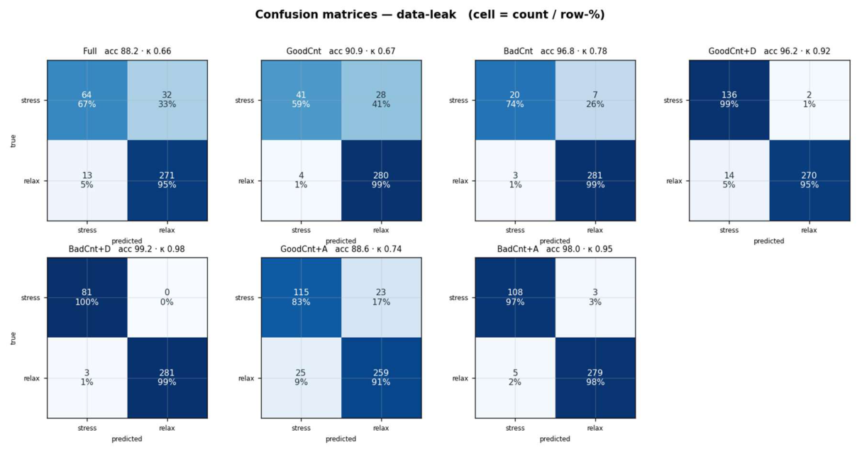
Figure 2.
Confusion matrixes for non-leak cases.
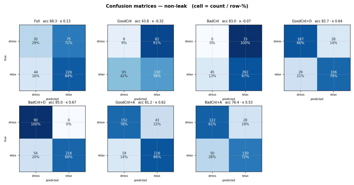

Table 1.
Overall performance across the 2×7 design. Prev. = prevalence of the stress class in the test set. ROC-AUC was logged only for the non-leak runs.
Table 1.
Overall performance across the 2×7 design. Prev. = prevalence of the stress class in the test set. ROC-AUC was logged only for the non-leak runs.
| Condition | Split | N | Prev. | Acc | Bal.Acc | κ | MCC | ROC-AUC | macro-F1 | wtd-F1 | G-mean |
| Data-leak | Full | 380 | 0.25 | 0.882 | 0.810 | 0.664 | 0.671 | – | 0.832 | 0.877 | 0.798 |
| Data-leak | Good Count | 353 | 0.20 | 0.909 | 0.790 | 0.668 | 0.690 | – | 0.833 | 0.902 | 0.765 |
| Data-leak | Bad Count | 311 | 0.09 | 0.968 | 0.865 | 0.783 | 0.786 | – | 0.891 | 0.967 | 0.856 |
| Data-leak | Good Count + Dummy | 422 | 0.33 | 0.962 | 0.968 | 0.916 | 0.918 | – | 0.958 | 0.963 | 0.968 |
| Data-leak | Bad Count + Dummy | 365 | 0.22 | 0.992 | 0.995 | 0.977 | 0.977 | – | 0.988 | 0.992 | 0.995 |
| Data-leak | Good Count + Aug | 422 | 0.33 | 0.886 | 0.873 | 0.743 | 0.743 | – | 0.871 | 0.886 | 0.872 |
| Data-leak | Bad Count + Aug | 395 | 0.28 | 0.980 | 0.978 | 0.950 | 0.950 | – | 0.975 | 0.980 | 0.978 |
| Non-leak | Full | 375 | 0.28 | 0.683 | 0.561 | 0.135 | 0.139 | 0.643 | 0.563 | 0.664 | 0.489 |
| Non-leak | Good Count | 315 | 0.29 | 0.438 | 0.333 | -0.320 | -0.321 | 0.282 | 0.339 | 0.449 | 0.227 |
| Non-leak | Bad Count | 352 | 0.04 | 0.830 | 0.433 | -0.068 | -0.081 | 0.518 | 0.453 | 0.868 | 0.000 |
| Non-leak | Good Count + Dummy | 330 | 0.59 | 0.827 | 0.821 | 0.642 | 0.642 | 0.881 | 0.821 | 0.827 | 0.820 |
| Non-leak | Bad Count + Dummy | 360 | 0.25 | 0.850 | 0.900 | 0.667 | 0.707 | 0.996 | 0.829 | 0.859 | 0.894 |
| Non-leak | Good Count + Aug | 330 | 0.59 | 0.812 | 0.819 | 0.622 | 0.628 | 0.891 | 0.810 | 0.814 | 0.818 |
| Non-leak | Bad Count + Aug | 330 | 0.46 | 0.764 | 0.768 | 0.529 | 0.534 | 0.778 | 0.763 | 0.764 | 0.766 |
Table 2.
Per-class performance and confusion-matrix counts.
| Condition | Split | Sens. (stress) | Spec. (relax) | Prec. (stress) | F1(stress) | Prec.(relax) | F1(relax) | TP | FN | FP | TN |
| Data-leak | Full | 0.667 | 0.954 | 0.831 | 0.740 | 0.894 | 0.923 | 64 | 32 | 13 | 271 |
| Data-leak | Good Count | 0.594 | 0.986 | 0.911 | 0.719 | 0.909 | 0.946 | 41 | 28 | 4 | 280 |
| Data-leak | Bad Count | 0.741 | 0.989 | 0.870 | 0.800 | 0.976 | 0.983 | 20 | 7 | 3 | 281 |
| Data-leak | Good Count + Dummy | 0.986 | 0.951 | 0.907 | 0.944 | 0.993 | 0.971 | 136 | 2 | 14 | 270 |
| Data-leak | Bad Count + Dummy | 1.000 | 0.989 | 0.964 | 0.982 | 1.000 | 0.995 | 81 | 0 | 3 | 281 |
| Data-leak | Good Count + Aug | 0.833 | 0.912 | 0.821 | 0.827 | 0.918 | 0.915 | 115 | 23 | 25 | 259 |
| Data-leak | Bad Count + Aug | 0.973 | 0.982 | 0.956 | 0.964 | 0.989 | 0.986 | 108 | 3 | 5 | 279 |
| Non-leak | Full | 0.286 | 0.837 | 0.405 | 0.335 | 0.751 | 0.792 | 30 | 75 | 44 | 226 |
| Non-leak | Good Count | 0.089 | 0.578 | 0.078 | 0.083 | 0.613 | 0.595 | 8 | 82 | 95 | 130 |
| Non-leak | Bad Count | 0.000 | 0.867 | 0.000 | 0.000 | 0.951 | 0.907 | 0 | 15 | 45 | 292 |
| Non-leak | Good Count + Dummy | 0.856 | 0.785 | 0.852 | 0.854 | 0.791 | 0.788 | 167 | 28 | 29 | 106 |
| Non-leak | Bad Count + Dummy | 1.000 | 0.800 | 0.625 | 0.769 | 1.000 | 0.889 | 90 | 0 | 54 | 216 |
| Non-leak | Good Count + Aug | 0.779 | 0.859 | 0.889 | 0.831 | 0.730 | 0.789 | 152 | 43 | 19 | 116 |
| Non-leak | Bad Count + Aug | 0.813 | 0.722 | 0.709 | 0.758 | 0.823 | 0.769 | 122 | 28 | 50 | 130 |
Table 3.
Accuracy-based training dynamics across the 2×7 design.
| Condition | Split | Best test acc | @epoch | Final test acc | Best F1 | Best κ | Final train acc | Train-test gap | Epochs to 95% best |
| Data-leak | Full | 0.913 | 372 | 0.882 | 0.912 | 0.763 | 0.999 | 0.118 | 13 |
| Data-leak | Good Count | 0.929 | 659 | 0.909 | 0.925 | 0.752 | 0.999 | 0.090 | 12 |
| Data-leak | Bad Count | 0.981 | 961 | 0.968 | 0.980 | 0.870 | 1.000 | 0.032 | 9 |
| Data-leak | Good Count + Dummy | 0.972 | 883 | 0.962 | 0.972 | 0.936 | 0.999 | 0.037 | 49 |
| Data-leak | Bad Count + Dummy | 1.000 | 129 | 0.992 | 1.000 | 1.000 | 1.000 | 0.008 | 7 |
| Data-leak | Good Count + Aug | 0.922 | 125 | 0.886 | 0.921 | 0.819 | 0.999 | 0.113 | 24 |
| Data-leak | Bad Count + Aug | 0.992 | 444 | 0.980 | 0.992 | 0.981 | 1.000 | 0.020 | 15 |
| Non-leak | Full | 0.803 | 4 | 0.683 | 0.783 | 0.435 | 0.999 | 0.317 | 2 |
| Non-leak | Good Count | 0.711 | 1 | 0.438 | 0.615 | 0.030 | 1.000 | 0.562 | 1 |
| Non-leak | Bad Count | 0.867 | 1 | 0.830 | 0.894 | 0.106 | 1.000 | 0.171 | 1 |
| Non-leak | Good Count + Dummy | 0.885 | 202 | 0.827 | 0.886 | 0.767 | 0.998 | 0.171 | 86 |
| Non-leak | Bad Count + Dummy | 0.972 | 221 | 0.850 | 0.973 | 0.929 | 0.999 | 0.149 | 54 |
| Non-leak | Good Count + Aug | 0.861 | 925 | 0.812 | 0.862 | 0.719 | 0.995 | 0.183 | 126 |
| Non-leak | Bad Count + Aug | 0.809 | 682 | 0.764 | 0.809 | 0.621 | 0.999 | 0.236 | 38 |
Table 4.
Label entropy and mutual-information diagnostics across the 2×7 design (bits unless stated).
Table 4.
Label entropy and mutual-information diagnostics across the 2×7 design (bits unless stated).
| Condition | Split | H(Y) | I(Y;Ŷ) | I/H(Y) | H(Y | Ŷ) | NMI√ | AMI |
| Data-leak | Full | 0.815 | 0.295 | 0.361 | 0.521 | 0.383 | 0.360 | 0.437 |
| Data-leak | Good Count | 0.713 | 0.274 | 0.385 | 0.439 | 0.438 | 0.383 | 0.323 |
| Data-leak | Bad Count | 0.426 | 0.232 | 0.544 | 0.194 | 0.576 | 0.541 | 0.160 |
| Data-leak | Good Count + Dummy | 0.912 | 0.712 | 0.781 | 0.200 | 0.770 | 0.758 | 0.197 |
| Data-leak | Bad Count + Dummy | 0.764 | 0.713 | 0.933 | 0.051 | 0.924 | 0.915 | 0.055 |
| Data-leak | Good Count + Aug | 0.912 | 0.415 | 0.455 | 0.497 | 0.454 | 0.452 | 0.460 |
| Data-leak | Bad Count + Aug | 0.857 | 0.721 | 0.842 | 0.136 | 0.839 | 0.835 | 0.130 |
| Non-leak | Full | 0.856 | 0.013 | 0.015 | 0.842 | 0.017 | 0.013 | 0.754 |
| Non-leak | Good Count | 0.863 | 0.086 | 0.100 | 0.777 | 0.097 | 0.092 | 0.961 |
| Non-leak | Bad Count | 0.254 | 0.009 | 0.034 | 0.245 | 0.023 | 0.011 | 0.430 |
| Non-leak | Good Count + Dummy | 0.976 | 0.317 | 0.324 | 0.659 | 0.325 | 0.323 | 0.606 |
| Non-leak | Bad Count + Dummy | 0.811 | 0.429 | 0.529 | 0.382 | 0.484 | 0.441 | 0.396 |
| Non-leak | Good Count + Aug | 0.976 | 0.309 | 0.317 | 0.666 | 0.313 | 0.308 | 0.619 |
| Non-leak | Bad Count + Aug | 0.994 | 0.218 | 0.219 | 0.776 | 0.219 | 0.217 | 0.714 |
Table 5.
Cross-entropy training-loss dynamics (nats).
| Condition | Split | Train CE (final) | Test CE (final) | Min test CE | @epoch | Gap@best | Gap (final) | CE rise (final-min) | p(true)@best |
| Data-leak | Full | 0.114 | 0.350 | 0.235 | 293 | 0.103 | 0.236 | 0.115 | 0.791 |
| Data-leak | Good Count | 0.089 | 0.575 | 0.242 | 154 | 0.107 | 0.485 | 0.333 | 0.785 |
| Data-leak | Bad Count | 0.013 | 0.156 | 0.083 | 47 | 0.027 | 0.143 | 0.074 | 0.921 |
| Data-leak | Good Count + Dummy | 0.100 | 0.130 | 0.088 | 726 | -0.017 | 0.030 | 0.042 | 0.916 |
| Data-leak | Bad Count + Dummy | 0.021 | 0.017 | 0.003 | 811 | -0.016 | -0.004 | 0.014 | 0.997 |
| Data-leak | Good Count + Aug | 0.121 | 0.325 | 0.254 | 235 | 0.096 | 0.204 | 0.071 | 0.776 |
| Data-leak | Bad Count + Aug | 0.035 | 0.048 | 0.032 | 964 | -0.049 | 0.013 | 0.015 | 0.968 |
| Non-leak | Full | 0.191 | 1.072 | 0.418 | 4 | -0.022 | 0.881 | 0.654 | 0.658 |
| Non-leak | Good Count | 0.096 | 3.905 | 0.687 | 2 | 0.311 | 3.809 | 3.217 | 0.503 |
| Non-leak | Bad Count | 0.043 | 1.359 | 0.264 | 1 | -0.071 | 1.316 | 1.096 | 0.768 |
| Non-leak | Good Count + Dummy | 0.170 | 1.059 | 0.553 | 234 | 0.353 | 0.889 | 0.506 | 0.575 |
| Non-leak | Bad Count + Dummy | 0.047 | 0.389 | 0.087 | 221 | 0.021 | 0.342 | 0.302 | 0.917 |
| Non-leak | Good Count + Aug | 0.182 | 0.548 | 0.371 | 158 | 0.151 | 0.366 | 0.177 | 0.690 |
| Non-leak | Bad Count + Aug | 0.051 | 0.979 | 0.546 | 411 | 0.472 | 0.928 | 0.433 | 0.579 |
Table 6.
Weight-matrix spectral entropy and effective rank.
| Condition | Split | L1 spec-H | L1 eff-rank | L1 nER | L2 spec-H | L2 eff-rank | L2 nER | BNγ nH | Mean nER |
| Data-leak | Full | 5.179 | 36.2 | 0.575 | 4.592 | 24.1 | 0.754 | 0.997 | 0.679 |
| Data-leak | Good Count | 5.191 | 36.5 | 0.580 | 4.537 | 23.2 | 0.725 | 0.995 | 0.677 |
| Data-leak | Bad Count | 5.054 | 33.2 | 0.527 | 4.544 | 23.3 | 0.729 | 0.993 | 0.634 |
| Data-leak | Good Count + Dummy | 5.194 | 36.6 | 0.581 | 4.536 | 23.2 | 0.725 | 0.996 | 0.685 |
| Data-leak | Bad Count + Dummy | 5.078 | 33.8 | 0.536 | 4.457 | 22.0 | 0.686 | 0.995 | 0.641 |
| Data-leak | Good Count + Aug | 5.138 | 35.2 | 0.559 | 4.527 | 23.1 | 0.721 | 0.996 | 0.674 |
| Data-leak | Bad Count + Aug | 5.074 | 33.7 | 0.535 | 4.493 | 22.5 | 0.704 | 0.997 | 0.651 |
| Non-leak | Full | 5.099 | 34.3 | 0.544 | 4.455 | 21.9 | 0.685 | 0.994 | 0.670 |
| Non-leak | Good Count | 5.126 | 34.9 | 0.554 | 4.523 | 23.0 | 0.718 | 0.995 | 0.679 |
| Non-leak | Bad Count | 5.018 | 32.4 | 0.514 | 4.535 | 23.2 | 0.724 | 0.993 | 0.646 |
| Non-leak | Good Count + Dummy | 5.138 | 35.2 | 0.559 | 4.548 | 23.4 | 0.731 | 0.998 | 0.700 |
| Non-leak | Bad Count + Dummy | 5.076 | 33.7 | 0.535 | 4.496 | 22.6 | 0.705 | 0.996 | 0.660 |
| Non-leak | Good Count + Aug | 5.120 | 34.8 | 0.552 | 4.533 | 23.2 | 0.724 | 0.998 | 0.684 |
| Non-leak | Bad Count + Aug | 5.044 | 33.0 | 0.524 | 4.464 | 22.1 | 0.690 | 0.997 | 0.643 |
Table 7.
SHAP explanation entropy, non-leak models (63 features = 21 channels × 3 statistics).
| Split | Feat. H (bits) | Feat. evenness | Eff. #feat | Top-1 share | Chan. H (bits) | Chan. evenness | Eff. #chan | Per-sample H |
| Full | 5.765 | 0.965 | 54.4 | 0.037 | 4.285 | 0.976 | 19.5 | 5.25 ± 0.15 |
| Good Count | 5.682 | 0.951 | 51.4 | 0.067 | 4.243 | 0.966 | 18.9 | 5.10 ± 0.25 |
| Bad Count | 5.599 | 0.937 | 48.5 | 0.053 | 4.182 | 0.952 | 18.2 | 5.00 ± 0.21 |
| Good Count + Dummy | 5.780 | 0.967 | 54.9 | 0.053 | 4.313 | 0.982 | 19.9 | 5.20 ± 0.20 |
| Bad Count + Dummy | 5.628 | 0.942 | 49.5 | 0.058 | 4.216 | 0.960 | 18.6 | 5.05 ± 0.21 |
| Good Count + Aug | 5.777 | 0.967 | 54.8 | 0.037 | 4.316 | 0.983 | 19.9 | 5.20 ± 0.18 |
| Bad Count + Aug | 5.612 | 0.939 | 48.9 | 0.063 | 4.232 | 0.964 | 18.8 | 5.05 ± 0.18 |
Table 8.
Comparison with published EEGMAT classification studies.
| Study | Task | Features / model | Evaluation | Accuracy |
| [10] (dataset) | defines 26 good / 10 bad counters | Fourier power, coherence, DFA | descriptive (no classifier) | – |
| [13] | rest vs. task | 8 feats/electrode + stacked LSTM | windowed random split | ≈93% |
| [14] | rest vs. task + difficulty | rhythm energy/entropy + SVM/DT/QDA | windowed CV | ≈90%+ |
| [16] | mental-arithmetic task | multi-entropy + RNN/LSTM/BLSTM/GRU | windowed split | high-90s% |
| [12] | rest vs. task (BCS/DCS) | 5-entropy fusion + ConvLSTM; MI + BLSTM | windowed 80/20 split | 99.72% / 97.45% |
| [18] | good vs. bad counters | FRLP/triangle-pooling + INCA + SVM | leave-one-subject-out | 93.40% |
| [17] | rest vs. calc; good vs. bad | EMD sub-bands + random forest + XAI | subject-dependent | 99.30% / 98.33% |
| [17] | rest vs. calc; good vs. bad | EMD sub-bands + random forest + XAI | leave-one-subject-out | 98.17±0.47% / 97.19±0.95% |
| This work | relaxed vs. one stress state | 3 stats/channel + MLP (63-64-32-2) | with subject leakage | 88.2-99.2% (mean 94.0%) |
| This work | relaxed vs. one stress state | 3 stats/channel + MLP (63-64-32-2) | subject-respecting split | 43.8-85.0% (mean 74.3%) |
Disclaimer/Publisher’s Note: The statements, opinions and data contained in all publications are solely those of the individual author(s) and contributor(s) and not of MDPI and/or the editor(s). MDPI and/or the editor(s) disclaim responsibility for any injury to people or property resulting from any ideas, methods, instructions or products referred to in the content. |
© 2026 by the authors. Licensee MDPI, Basel, Switzerland. This article is an open access article distributed under the terms and conditions of the Creative Commons Attribution (CC BY) license (http://creativecommons.org/licenses/by/4.0/).
Copyright: This open access article is published under a Creative Commons CC BY 4.0 license, which permit the free download, distribution, and reuse, provided that the author and preprint are cited in any reuse.