

Submitted:
14 September 2026
Posted:
15 September 2026
You are already at the latest version
Abstract
In safety-critical applications such as industrial fault diagnosis, classification accuracy alone is not sufficient — the reliability of a model’s confidence estimates is equally important. In this work, which is a continuation of research on electric motor fault classification presented in a companion paper, pre-trained probabilistic prediction models were applied to motor state classification, and their predictive uncertainty was subsequently modelled and compared using five strategies: (1) native probabilistic outputs of single models, (2) tree level variance decomposition for Random Forest, (3) bootstrap ensemble aggregation for frequentist classifiers, (4) Markov Chain Monte Carlo (MCMC) posterior sampling for Bayesian Softmax Regression, and (5) Monte Carlo Dropout for LSTM networks. These strategies were evaluated on two complementary data representations — statistical feature vectors (56 test samples) and raw signal time windows (22372 test windows) — using six metrics: accuracy, Negative Log-Likelihood (NLL), Brier Score, Expected Calibration Error (ECE), average predictive entropy, and average epistemic variance. Additionally, an Error Detection AUC metric was introduced to assess the practical utility of uncertainty for flagging misclassifications. Taking the best results from each evaluation set: on the statistical feature set, the Bayesian Softmax model achieved the best calibration (ECE = 0.060), the lowest NLL (0.257) and Brier Score (0.157), while Random Forest attained both the highest accuracy (89.5%) and the highest Error Detection AUC (0.909). On the time series set, LSTM with MC Dropout achieved the best results across all reported metrics simultaneously: accuracy of 95.0%, NLL of 0.117, Brier Score of 0.071, near-perfect calibration (ECE = 0.015), and an Error Detection AUC of 0.945. Convergence of the MCMC sampler was confirmed by R-hat values of 1.000 for all parameters and effective sample sizes exceeding 3000. The results indicate that bootstrap ensembles consistently improve uncertainty quality across all base classifiers, and that Bayesian methods provide better calibration even when accuracy is not maximal.
Keywords:
uncertainty quantification
; calibration
; Expected Calibration Error
; Brier Score
; bootstrap ensemble
; Monte Carlo Dropout
; Bayesian inference
; fault diagnosis
; predictive maintenance
1. Introduction
Machine learning classifiers deployed in industrial fault diagnosis must satisfy a dual requirement: high accuracy and reliable quantification of predictive uncertainty [3,5]. In the context of electric motor condition monitoring, an overconfident misclassification — for example, declaring a mechanically damaged motor healthy with 99% confidence — can lead to catastrophic equipment failure and endanger personnel safety [18]. Uncertainty estimation can in such cases serve as an explainability mechanism, enabling classification with rejection — the model rejects low-confidence predictions and routes them to human review instead of making a risky automatic decision [4].
Although the accuracy of machine learning models for motor fault classification has been the subject of numerous comparative studies [1,5], comparatively little attention has been devoted to a systematic evaluation of the quality of their uncertainty estimates. Traditional evaluation pipelines report accuracy, precision, recall, and F1-score, but these metrics provide no information on whether a model’s softmax confidence actually corresponds to the true probability of correct classification [6]. A classifier achieving 95% accuracy may still be poorly calibrated if its confident predictions are frequently wrong or its uncertain predictions turn out to be typically correct.
Uncertainty in classification arises from two fundamentally different sources [7,9]. Aleatoric uncertainty is an irreducible property of the data, reflecting inherent overlap between class distributions. Epistemic uncertainty is a property of the model, arising from limited training data or model misspecification, and can in principle be reduced by collecting more data or improving the architecture. Different uncertainty quantification (UQ) strategies capture these sources to varying degrees [8]: native softmax probabilities conflate both sources; bootstrap ensembles primarily estimate epistemic uncertainty through inter-model disagreement; and fully Bayesian methods provide principled posterior predictive distributions [10,11].
In this study, classification models developed and optimised in a companion paper [1] — which presented a comparative analysis of machine learning algorithms, probabilistic models, and neural networks for DC motor fault classification — were used as a basis. The predictive uncertainty of these models was modelled using five UQ strategies across eleven classifier configurations. The three main contributions are:
- 1.
- Formalisation of an evaluation protocol for uncertainty quality in diagnostic classifiers, integrating six complementary metrics — accuracy, NLL, Brier Score, ECE, predictive entropy, and epistemic variance — together with an Error Detection AUC metric that directly measures the practical utility of uncertainty for identifying misclassifications.
- 2.
- Demonstration that bootstrap ensemble augmentation consistently improves uncertainty metrics for all tested base classifiers (Gaussian Naive Bayes, QDA, XGBoost), offering a low-cost pathway to better-calibrated predictions without changing the model architecture.
- 3.
- The first direct comparison of Bayesian MCMC (Bayesian Softmax Regression), Monte Carlo Dropout (LSTM), and frequentist ensemble methods on the same diagnostic dataset, enabling evidence-based selection of UQ strategies for industrial deployment.
The remainder of the paper is organised as follows. Section 2 reviews related work on uncertainty quantification in fault diagnosis. Section 3 describes the five uncertainty extraction methods and six evaluation metrics. Section 4 presents the experimental setup and data. Section 5 reports results for both experiments. Section 6 discusses practical implications, and Section 7 concludes the paper.
2. Related Work
2.1. Uncertainty Quantification in Deep Learning
The overconfidence problem in neural networks has been identified in the literature [6], where it was shown that modern deep networks are often poorly calibrated, with confidence levels that significantly exceed actual correctness rates. This observation has motivated a rich body of research on post-hoc calibration methods (temperature scaling, Platt scaling) and architectures with built-in calibration. A review of these methods, including a taxonomy of uncertainty sources and quantification techniques, can be found in [7,12].
Bayesian Neural Networks (BNN) represent a principled approach to uncertainty quantification by maintaining distributions over model weights instead of point estimates [13]. However, exact Bayesian inference in deep networks is computationally intractable, necessitating approximate methods. It has been shown that dropout applied at inference time — known as Monte Carlo Dropout — can be interpreted as variational inference in a deep Gaussian process, providing a computationally cheap approximation to Bayesian uncertainty [10]. As an alternative, deep ensembles have been proposed, demonstrating that training multiple networks with different initialisations yields competitive uncertainty estimates [11].
Bootstrap ensembles represent a classical non-parametric approach to uncertainty estimation [14]. By training B models on bootstrap samples from the training set, the variance across predictions approximates sampling uncertainty. Combined with proper calibration, this approach can generate high-quality confidence intervals [8].
2.2. Uncertainty in Fault Diagnosis
In the fault diagnosis community, uncertainty-aware methods have gained attention primarily in the context of out-of-distribution (OOD) data detection. Novel dissimilarity measures based on anomaly detection (ADD measures) have been proposed for quantifying the uncertainty of ML classifier performance on OOD data, demonstrating that the amplitude of the uncertainty band grows with increasing dissimilarity between training and test sets [15]. Uncertainty-aware deep ensembles have been applied to OOD detection in machinery fault diagnosis [16]. Sampling by dropout, BNN, and deep ensembles have also been compared for rotating machinery fault classification under scenarios involving both epistemic and aleatoric uncertainty [17]. In the context of calibration, a trustworthy Bayesian deep learning approach integrating -divergence for uncertainty decomposition in machinery diagnostics has been proposed [18].
Despite these advances, most studies evaluate uncertainty within a single methodological paradigm (e.g., exclusively BNN or exclusively ensembles). Comprehensive cross-paradigm comparisons on the same dataset remain rare, particularly for motor fault diagnosis. This study addresses that gap by evaluating Bayesian MCMC, MC Dropout, tree-level variance decomposition, and bootstrap ensembles within a unified experimental scheme.
3. Methods
3.1. Uncertainty Extraction Strategies
3.1.1. Native Probabilistic Outputs
All classifiers considered — trained and optimised in [1] — produce class probability vectors for each test sample . For Gaussian Naive Bayes (GNB), these probabilities derive from class posteriors via Bayes’ theorem. For Quadratic Discriminant Analysis (QDA), they arise from class-conditional Gaussian likelihoods with class-specific covariance matrices. For XGBoost, probabilities are obtained by applying softmax to the aggregation of leaf values in the boosted tree ensemble. These native outputs serve as the baseline uncertainty representation.
3.1.2. Tree-Level Variance Decomposition for Random Forest
In the Random Forest model, uncertainty is decomposed by leveraging the ensemble of T decision trees. Let denote the class k probability predicted by tree t for sample i. The mean probability and epistemic variance are:
The inter-tree variance directly measures disagreement among individual trees and serves as an estimator of epistemic uncertainty. This decomposition was implemented as the extract_rf_uncertainty method of the evaluation module.
3.1.3. Bootstrap Ensemble Aggregation
For classifiers that do not provide native ensemble decomposition (GNB, QDA, XGBoost), uncertainty is estimated via bootstrap ensembling. Given a training set of N samples, B bootstrap replicates are generated by sampling N points with replacement. A separate classifier is trained on each replicate, producing B probability vectors for each test sample:
The mean prediction and epistemic variance are then:
This strategy was implemented as the BootstrapEnsemble class with for GNB and QDA, and for XGBoost (reflecting its higher computational cost per model).
3.1.4. Bayesian MCMC Posterior Sampling
For the Bayesian Softmax Regression model, whose architecture and MCMC sampling procedure are described in [1], uncertainty is extracted from the posterior predictive distribution obtained via the NUTS sampler [19] in PyMC [20]. The model defines the class k probability for observation i as:
where is the weight matrix and the bias vector. Normal priors were placed on all parameters: and . Posterior inference was performed using the NUTS sampler with 4 independent chains, each generating 1000 tuning samples and 1000 posterior draws, with a target acceptance rate of 0.95.
Given posterior samples , the prediction for test sample under posterior draw s is:
The mean predictive probability and epistemic variance are computed over all posterior samples:
This approach provides a principled estimate of epistemic uncertainty grounded in the true posterior distribution, as opposed to the heuristic resampling of bootstrap methods.
3.1.5. Monte Carlo Dropout for LSTM
Following the MC Dropout approach [10], the LSTM network — whose dual-channel architecture (current and rotational speed) with an MC Dropout layer is described in [1] — employs Monte Carlo Dropout at inference time. Dropout layers with rate remain active during prediction, and stochastic forward passes are performed for each test sample. If denotes the softmax output of forward pass t:
MC Dropout approximates Bayesian inference through a variational Bernoulli distribution over the network weights, where the variance of stochastic outputs serves as an approximation to posterior predictive variance.
3.2. Evaluation Metrics
All metrics are computed on the test set. Let N denote the number of test samples, K the number of classes, the true class of sample i, and the predicted probability for class k.
3.2.1. Negative Log-Likelihood (NLL)
NLL measures the quality of the predicted probability distribution:
Lower values indicate that the model assigns higher probability to the correct class. NLL heavily penalises confident wrong predictions due to the logarithmic scale.
3.2.2. Brier Score
The multiclass Brier Score measures the mean squared error between predicted probabilities and one-hot encoded labels [21]:
Unlike NLL, the Brier Score is bounded in and provides a more stable gradient for incorrect confident predictions.
3.2.3. Expected Calibration Error (ECE)
ECE [6,22] partitions test predictions into equal-width bins based on the maximum predicted probability (confidence), then computes the weighted average discrepancy between bin-level confidence and accuracy:
where is the set of predictions in bin m, is the fraction of correct predictions in that bin, and is the average maximum predicted probability. An ECE of 0 indicates perfect calibration.
3.2.4. Predictive Entropy
The Shannon entropy of the predicted class distribution quantifies total predictive uncertainty (both aleatoric and epistemic):
Entropy equals 0 for a perfectly confident prediction and for a uniform distribution.
3.2.5. Average Epistemic Variance
For ensemble and Bayesian models, epistemic variance is computed as described in Section 3.1 and averaged over all test samples and classes:
This metric is only available for models providing multiple prediction instances (ensembles, MCMC draws, MC Dropout forward passes).
3.2.6. Error Detection AUC
The Error Detection AUC metric evaluates the practical utility of uncertainty as a misclassification detector. For each test sample, predictive entropy serves as the uncertainty score. Samples are labelled as “correct” or “incorrect” based on the classification outcome. The ROC curve is computed using uncertainty as the positive class score (higher uncertainty → greater probability of error), and the AUC is reported. A value of 1.0 means that all misclassifications have higher uncertainty than all correct classifications; 0.5 indicates random separation.
4. Experimental Setup
4.1. Dataset and Preprocessing
The experiments use the DUDU-BLDC dataset [2], a publicly available benchmark for diagnostic research on brushless DC motors with degrading magnets. The dataset was collected from Fein EC48 BLDC motors powered by the original 18 V, 3 Ah Li-ion battery pack and controlled via the Fein ASCM 18 QM PWM drive operating at 16 kHz. Two synchronised sensor channels were recorded: stator current (A) measured with an Allegro ACS712-20 Hall-effect current sensor and rotational speed (RPM) measured with a Lasergage A2108/LSR laser tachometer, both sampled at 50 kHz and segmented into 0.8 s windows.
Measurements were performed under four operating conditions representing distinct fault modes:
- Healthy — nominally healthy motor with no electrical or mechanical damage;
- Healthy_zip — electrically healthy motor with mechanical damage introduced via zip-tie rotor imbalance;
- Faulty — electrical degradation caused by partial rotor demagnetisation, no mechanical damage;
- Faulty_zip — combined electrical degradation (partial demagnetisation) and mechanical damage (zip-tie imbalance).
The raw dataset, distributed as CSV files following the TIER 4.0 protocol, contains 28 time- and frequency-domain features per record — including mean, standard deviation, maximum, RMS, peak-to-peak amplitude, skewness, kurtosis, crest factor, spectral centroid, spectrum area, and amplitudes at the 1×, 2×, and 3× rotational harmonics — computed independently for both current and speed channels. The dataset is released under the CC BY 4.0 licence (DOI: 10.5281/zenodo.15522163).
Two data representations were prepared for the present study:
Statistical feature set. Following the procedure described in [1], statistical features in the time and frequency domains were extracted from each signal segment. After removing highly correlated variables (correlation threshold 90%), 18 features remained. The set contains 128 training and 56 test samples (32 and 14 per class, respectively).
Time window set. Raw signals were segmented using a sliding window of 100 time steps × 2 features (current, RPM), corresponding to a 2 ms window at 50 kHz sampling frequency. After merging the training and validation sets, 124 644 training windows and 22 372 test windows were obtained (31 161 and 5593 per class, respectively).
4.2. Models Under Evaluation
All classification models used in this study were trained and optimised in [1]. On the statistical feature set, generative models (Gaussian Naive Bayes, QDA), ensemble tree models (Random Forest, XGBoost), and Bayesian Softmax Regression with MCMC posterior sampling were evaluated. On the time window set, an LSTM network with MC Dropout and a reference GNB model on flattened time windows were evaluated. Details of individual model architectures, hyperparameter optimisation procedures, and baseline accuracy are presented in [1]; the present work focuses exclusively on the extraction and comparison of predictive uncertainty.
To enable epistemic uncertainty estimation for models that natively return only point estimates (GNB, QDA, XGBoost), a bootstrap ensemble approach inspired by the Deep Ensembles method [11] was adopted and adapted to classical ML algorithms, following the procedure described in Section 2.5 of [1].
Table 1 summarises the models and associated uncertainty extraction strategies evaluated in each experiment.
5. Results
5.1. Uncertainty Comparison on the Statistical Feature Set
Table 2 presents the full uncertainty evaluation for all eight model configurations tested on the statistical feature set.
Figure 1.
Uncertainty intervals for the Random Forest model on the statistical feature set. Predictions sorted by sample index with uncertainty intervals ( std) derived from tree-level variance.
Figure 1.
Uncertainty intervals for the Random Forest model on the statistical feature set. Predictions sorted by sample index with uncertainty intervals ( std) derived from tree-level variance.
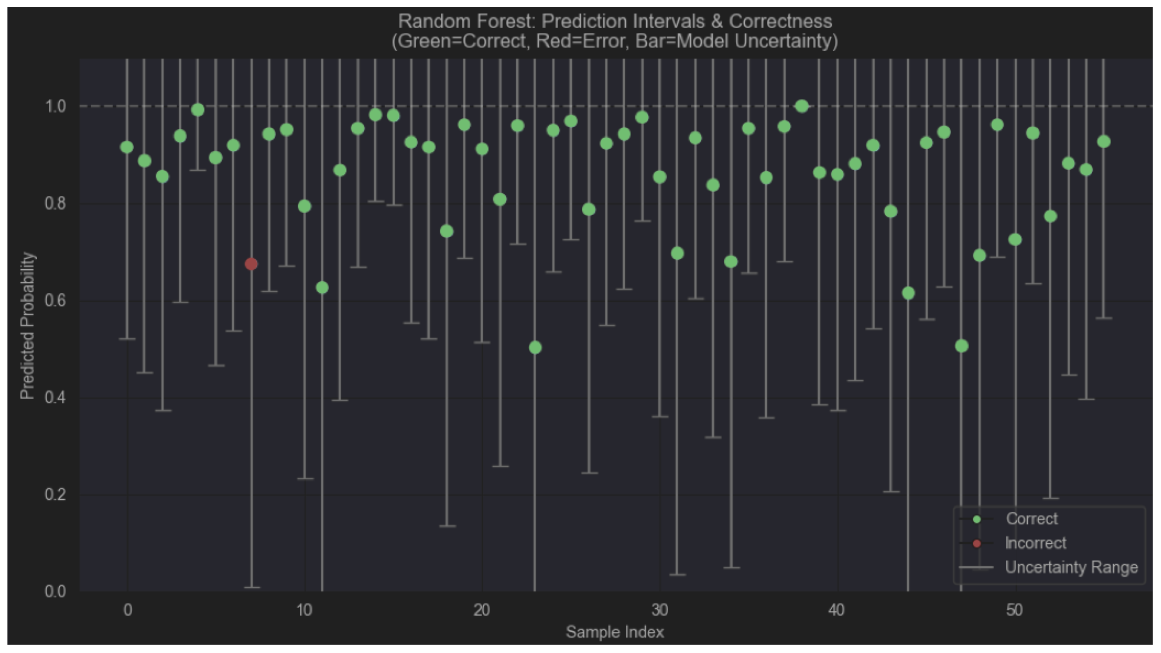
Figure 2.
Uncertainty intervals for XGBoost Bootstrap Ensemble () on the statistical feature set.
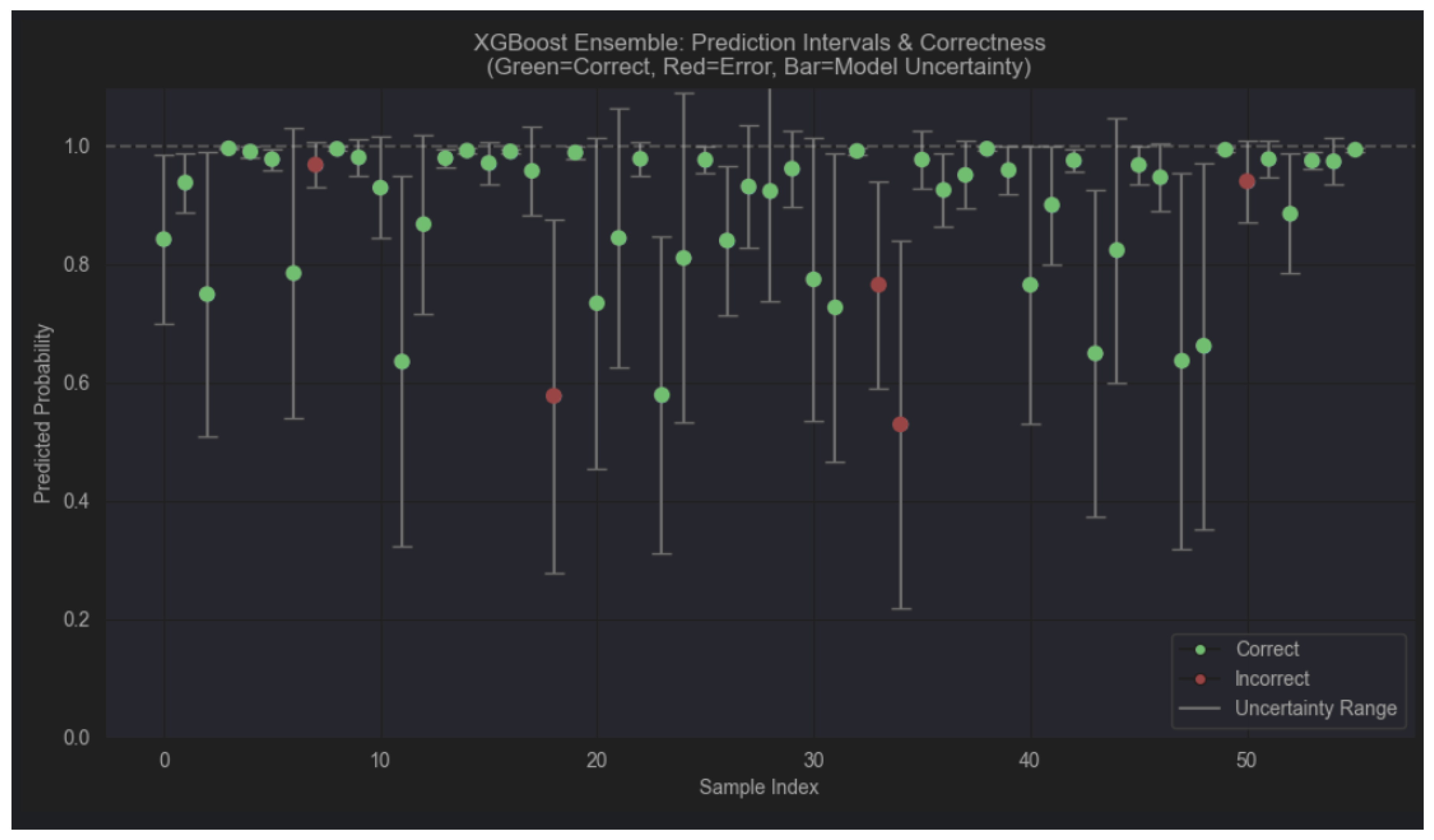
Figure 3.
Uncertainty intervals for GNB Bootstrap Ensemble () on the statistical feature set.
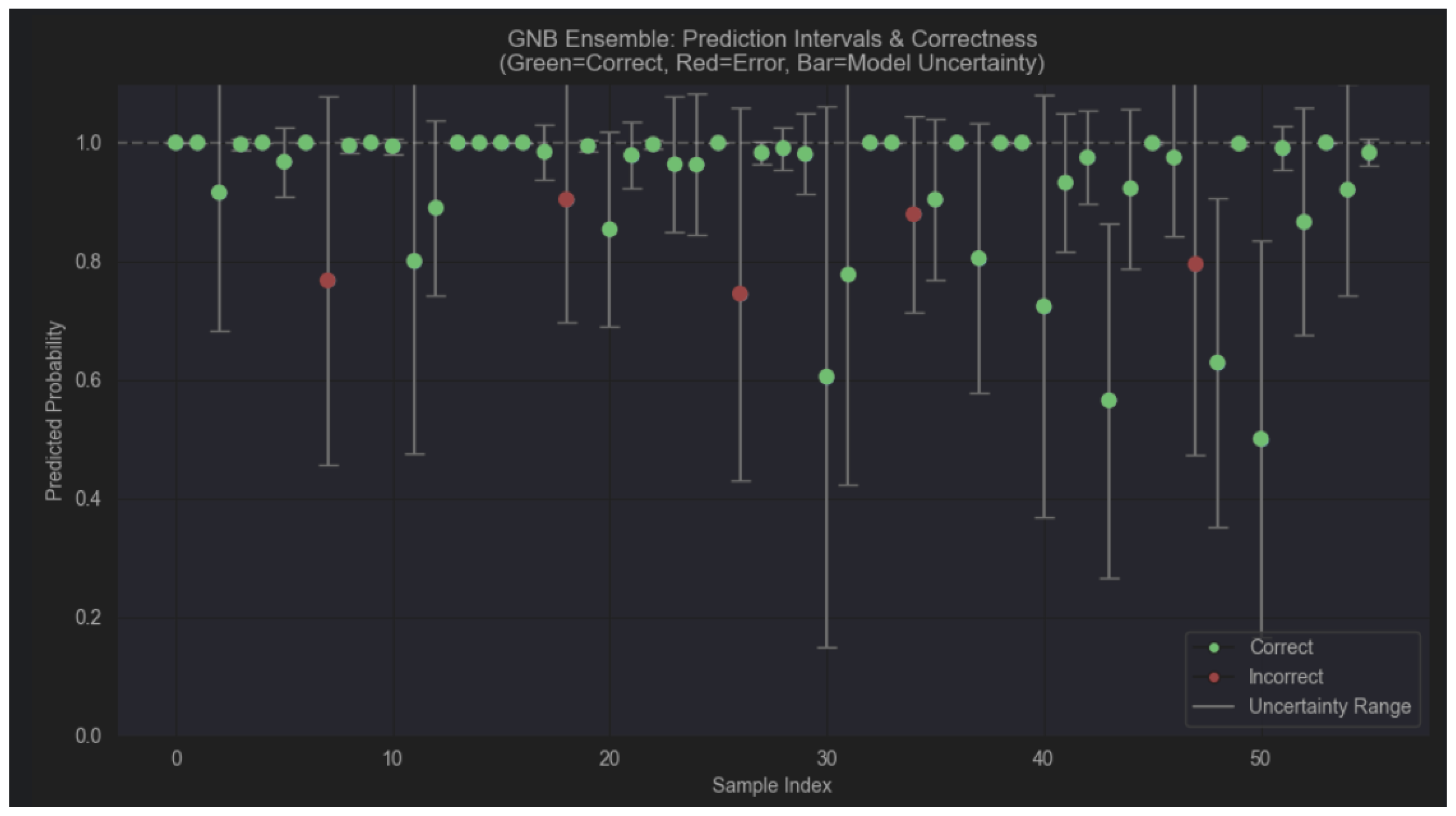
Figure 4.
Uncertainty intervals for QDA Bootstrap Ensemble () on the statistical feature set.
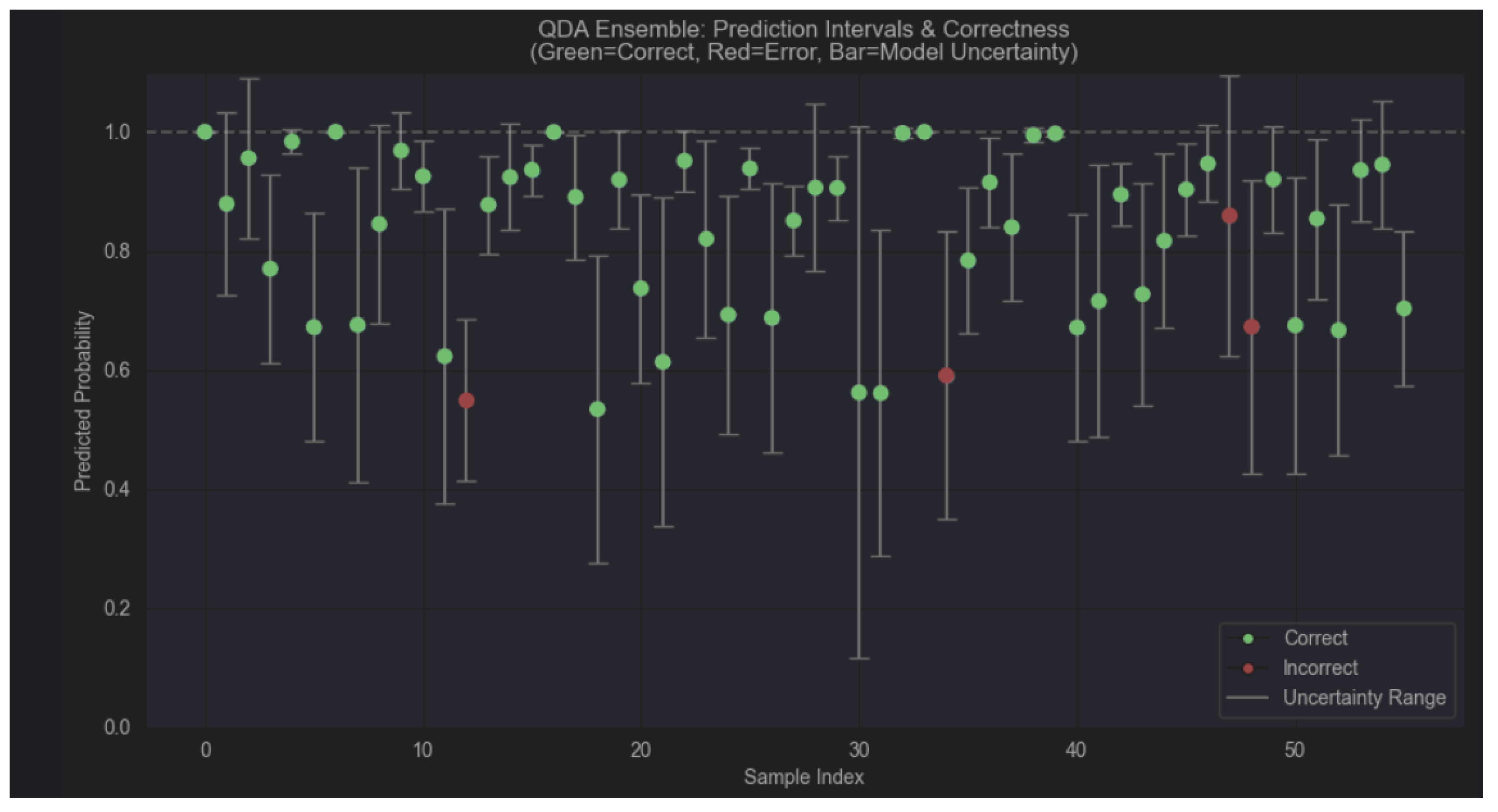
Figure 5.
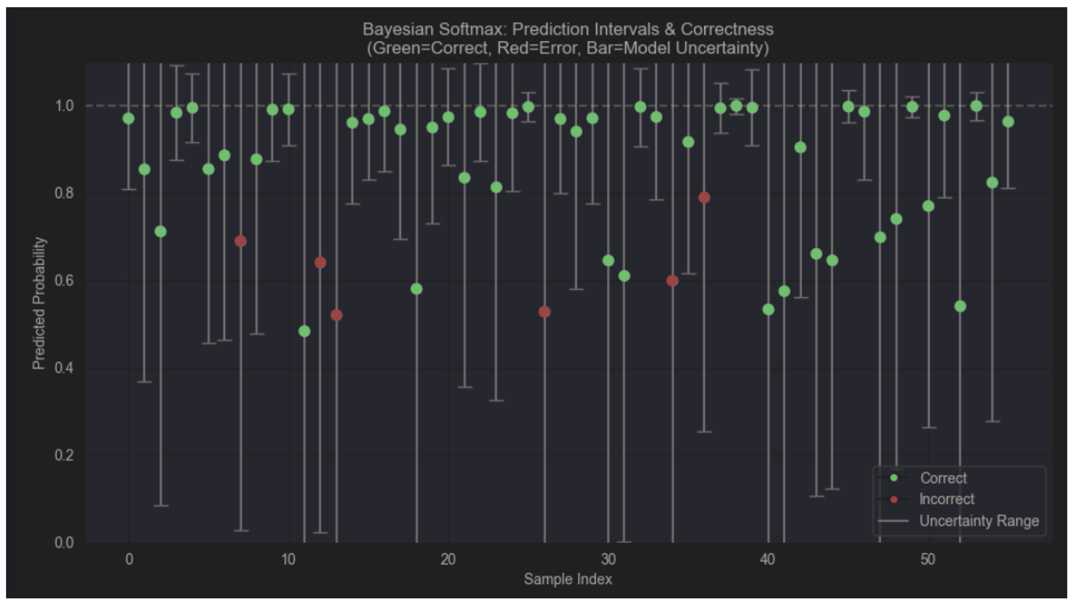
Uncertainty intervals for Bayesian Softmax Regression on the statistical feature set. Uncertainty intervals are derived from the variance of the posterior predictive distribution ( MCMC samples).
Figure 5.
Uncertainty intervals for Bayesian Softmax Regression on the statistical feature set. Uncertainty intervals are derived from the variance of the posterior predictive distribution ( MCMC samples).
Effect of bootstrap ensembling. Comparing single models with their ensemble counterparts reveals a generally positive but model-dependent effect on uncertainty metrics. For GNB, bootstrap ensembling reduced NLL from 0.564 to 0.413 (a 27% improvement), while ECE improved only marginally from 0.106 to 0.105, and Error Detection AUC reached 0.855. For XGBoost, ensembling improved the Error Detection AUC from 0.535 to 0.773 — a dramatic increase — albeit at the cost of a slight accuracy decrease from 0.868 to 0.875 and an increase in average entropy from 0.208 to 0.349, suggesting that the ensemble introduces greater predictive spread. The QDA Ensemble exhibited the opposite calibration trend: ECE increased from 0.103 to 0.108, suggesting that bootstrap resampling on a small dataset can introduce variance in covariance matrix estimation, degrading calibration for quadratic discriminant models.
Figure 6.
Predictive entropy distribution (KDE) on the statistical feature test set. XGBoost and Gaussian NB are the most confident models, while Random Forest produces the widest distribution despite its high accuracy. QDA Ensemble exhibits a pronounced bimodal structure, indicating a tendency towards either high confidence or high uncertainty.
Figure 6.
Predictive entropy distribution (KDE) on the statistical feature test set. XGBoost and Gaussian NB are the most confident models, while Random Forest produces the widest distribution despite its high accuracy. QDA Ensemble exhibits a pronounced bimodal structure, indicating a tendency towards either high confidence or high uncertainty.
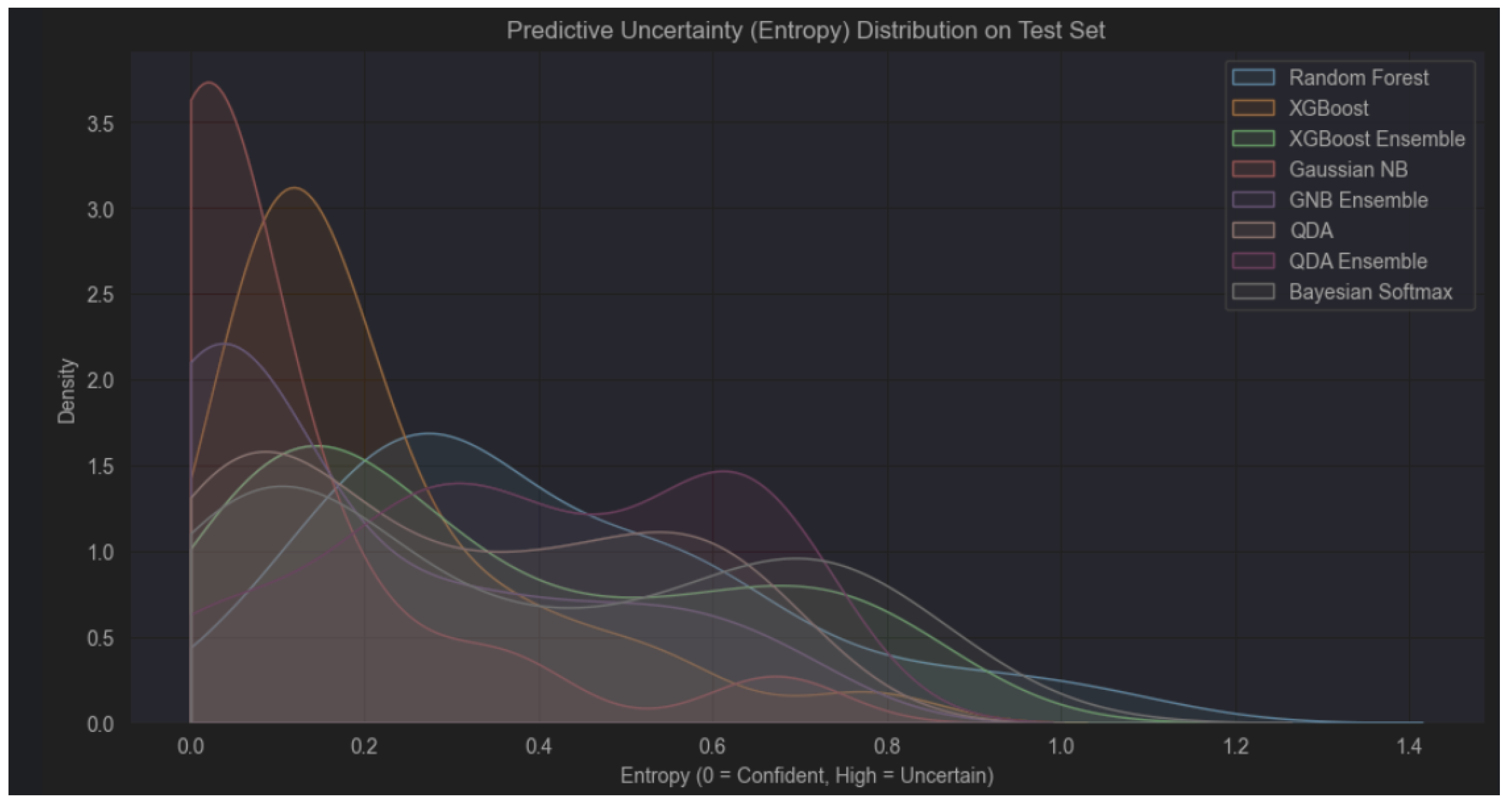
Figure 7.
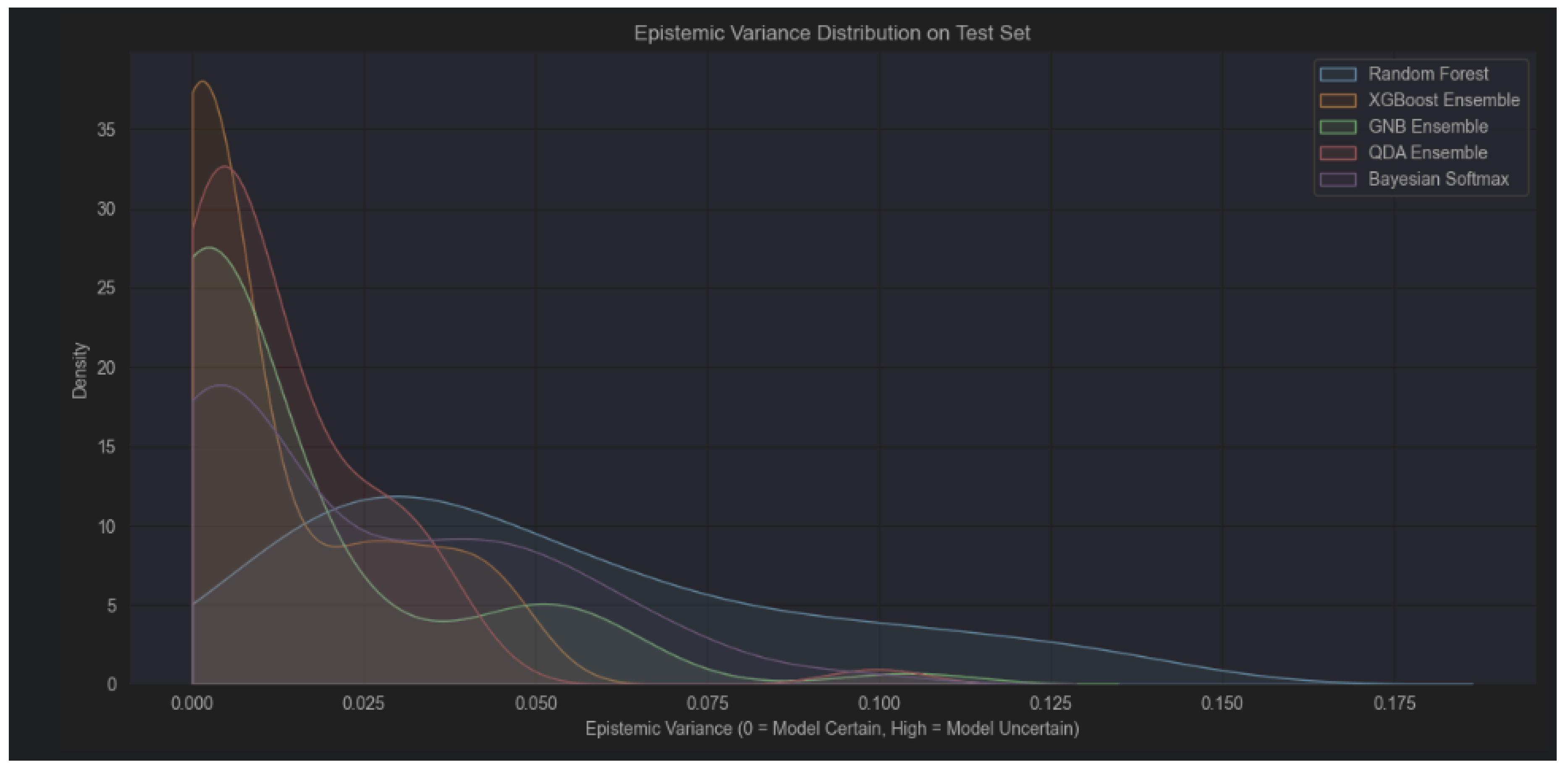
Epistemic variance distribution (KDE) on the statistical feature test set. Single deterministic models are excluded. Random Forest exhibits the heaviest tail, reflecting high inter-tree disagreement on ambiguous samples. GNB Ensemble and Bayesian Softmax produce the most compact distributions, consistent with their superior calibration scores.
Figure 7.
Epistemic variance distribution (KDE) on the statistical feature test set. Single deterministic models are excluded. Random Forest exhibits the heaviest tail, reflecting high inter-tree disagreement on ambiguous samples. GNB Ensemble and Bayesian Softmax produce the most compact distributions, consistent with their superior calibration scores.
5.2. Uncertainty Comparison on the Time Series Set
Table 3 presents the uncertainty evaluation for the three model configurations evaluated on the time window set.
LSTM with MC Dropout dominates across all six metrics. Its Error Detection AUC of 0.946 is the highest value observed in either experiment, indicating that MC Dropout variance concentrates precisely on misclassified samples. An ECE of 0.015 represents near-perfect calibration, far surpassing the best feature-set model (Bayesian Softmax at ECE = 0.051). An NLL of 0.117 is more than twice as good as the GNB Window variants (), confirming that the LSTM assigns substantially higher probability to the correct class.
Figure 8.
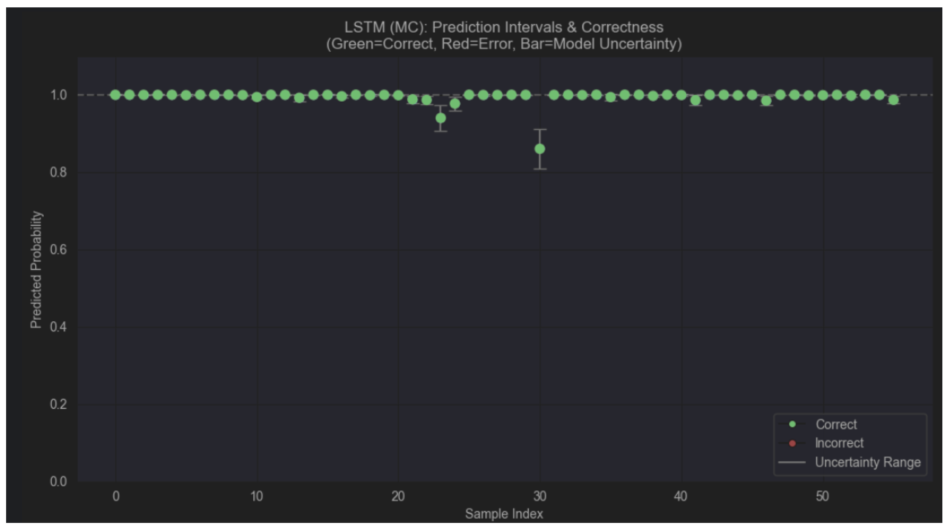
Uncertainty intervals for LSTM with MC Dropout ( forward passes) on the time series set. Uncertainty intervals are derived from the variance of stochastic forward passes.
Figure 8.
Uncertainty intervals for LSTM with MC Dropout ( forward passes) on the time series set. Uncertainty intervals are derived from the variance of stochastic forward passes.
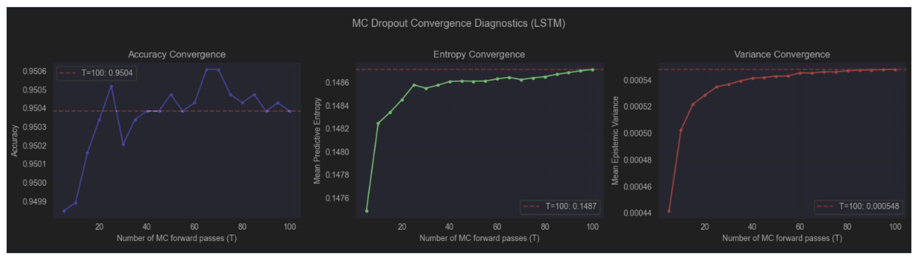
Unlike MCMC methods, MC Dropout does not produce chains amenable to R-hat or ESS analysis. Convergence is instead assessed by tracking how accuracy, predictive entropy, and epistemic variance stabilise as the number of stochastic forward passes T increases.
Figure 12 shows the evolution of all three statistics for . Accuracy stabilises almost immediately, fluctuating within a narrow band around the asymptotic value. Entropy and variance converge monotonically, reaching a plateau by approximately . The quantitative convergence summary confirms that all metrics change by less than 1% between and (accuracy: , entropy: , variance: ), satisfying the convergence criterion. A value of forward passes is therefore sufficient for reliable uncertainty estimation with this model.
Figure 9.
Uncertainty intervals for GNB Window Bootstrap Ensemble () on the time series set.
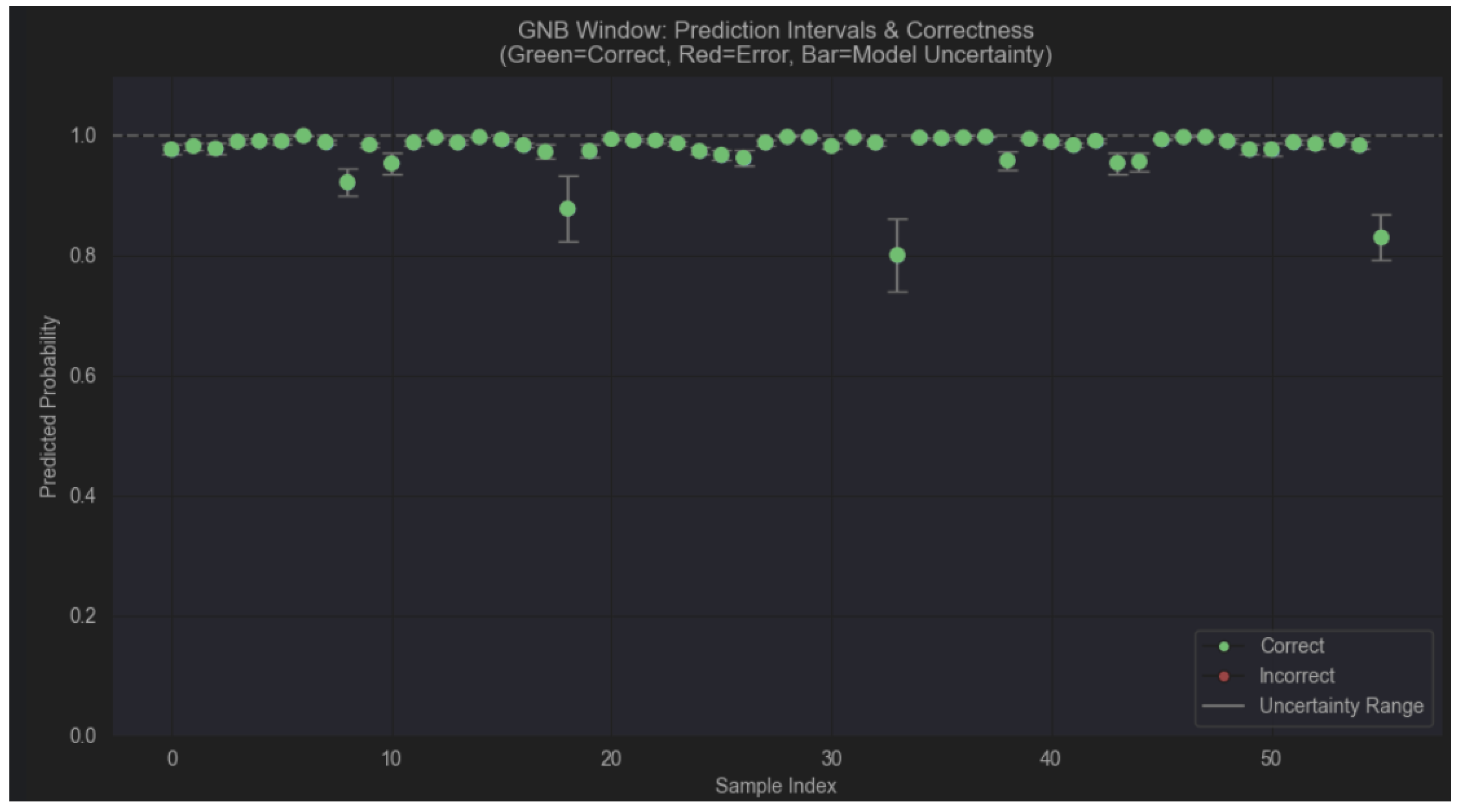
Both GNB Window variants exhibit nearly identical performance across all metrics, suggesting that bootstrap ensembling provides minimal benefit when the base classifier is a poor fit for the high-dimensional flattened time series representation ().
Figure 10.
Predictive entropy distribution (KDE) on the time series test set for LSTM (MC Dropout), GNB Window Ensemble, and GNB Window. All three models share a bimodal structure: a dominant peak near entropy = 0 (confident predictions) and a secondary plateau around entropy ≈ 0.65 (uncertain predictions), corresponding to samples near class boundaries. The LSTM exhibits a slightly sharper primary peak, indicating marginally higher overall confidence than the GNB variants, whose entropy distributions are nearly indistinguishable.
Figure 10.
Predictive entropy distribution (KDE) on the time series test set for LSTM (MC Dropout), GNB Window Ensemble, and GNB Window. All three models share a bimodal structure: a dominant peak near entropy = 0 (confident predictions) and a secondary plateau around entropy ≈ 0.65 (uncertain predictions), corresponding to samples near class boundaries. The LSTM exhibits a slightly sharper primary peak, indicating marginally higher overall confidence than the GNB variants, whose entropy distributions are nearly indistinguishable.
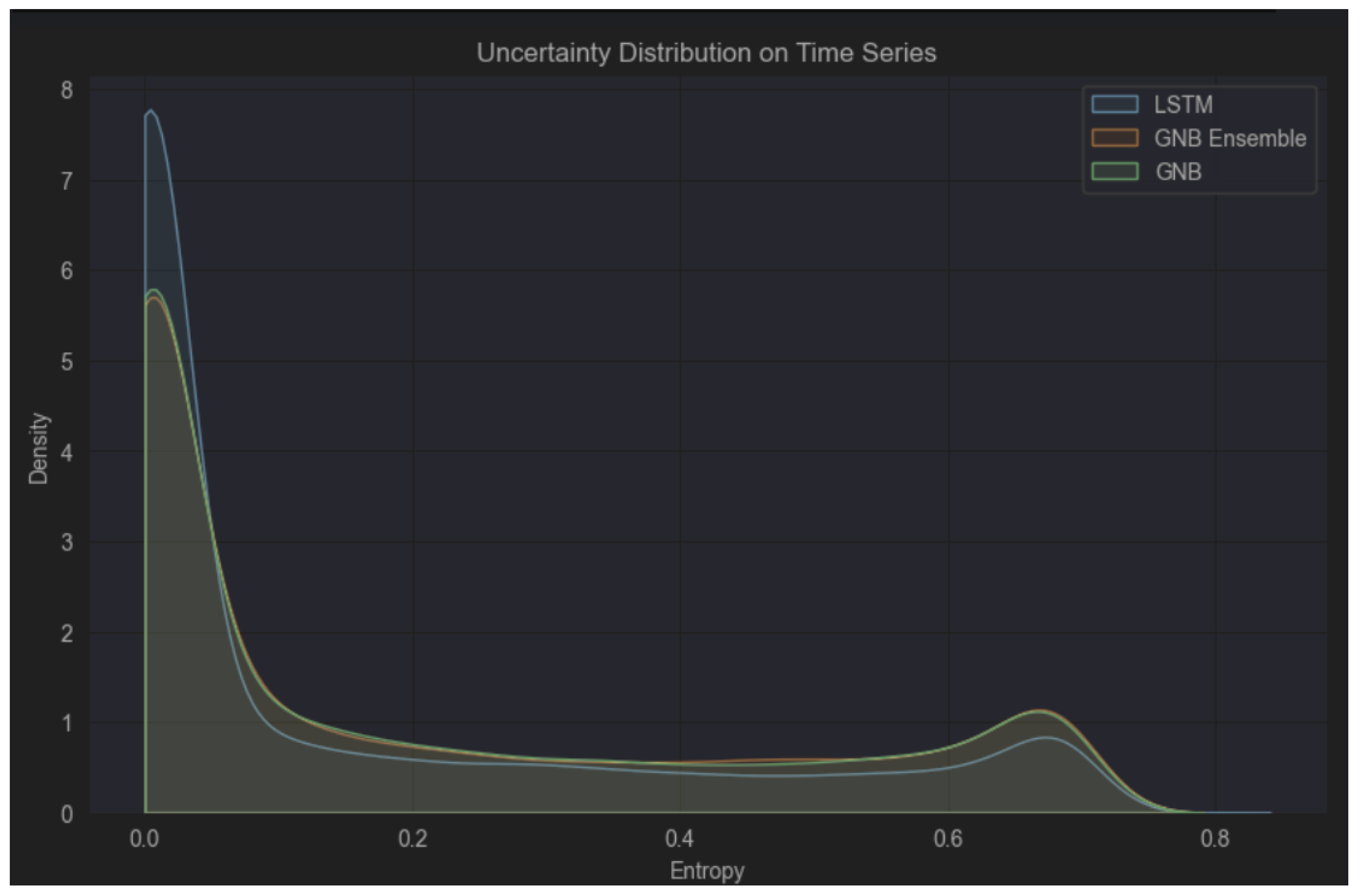
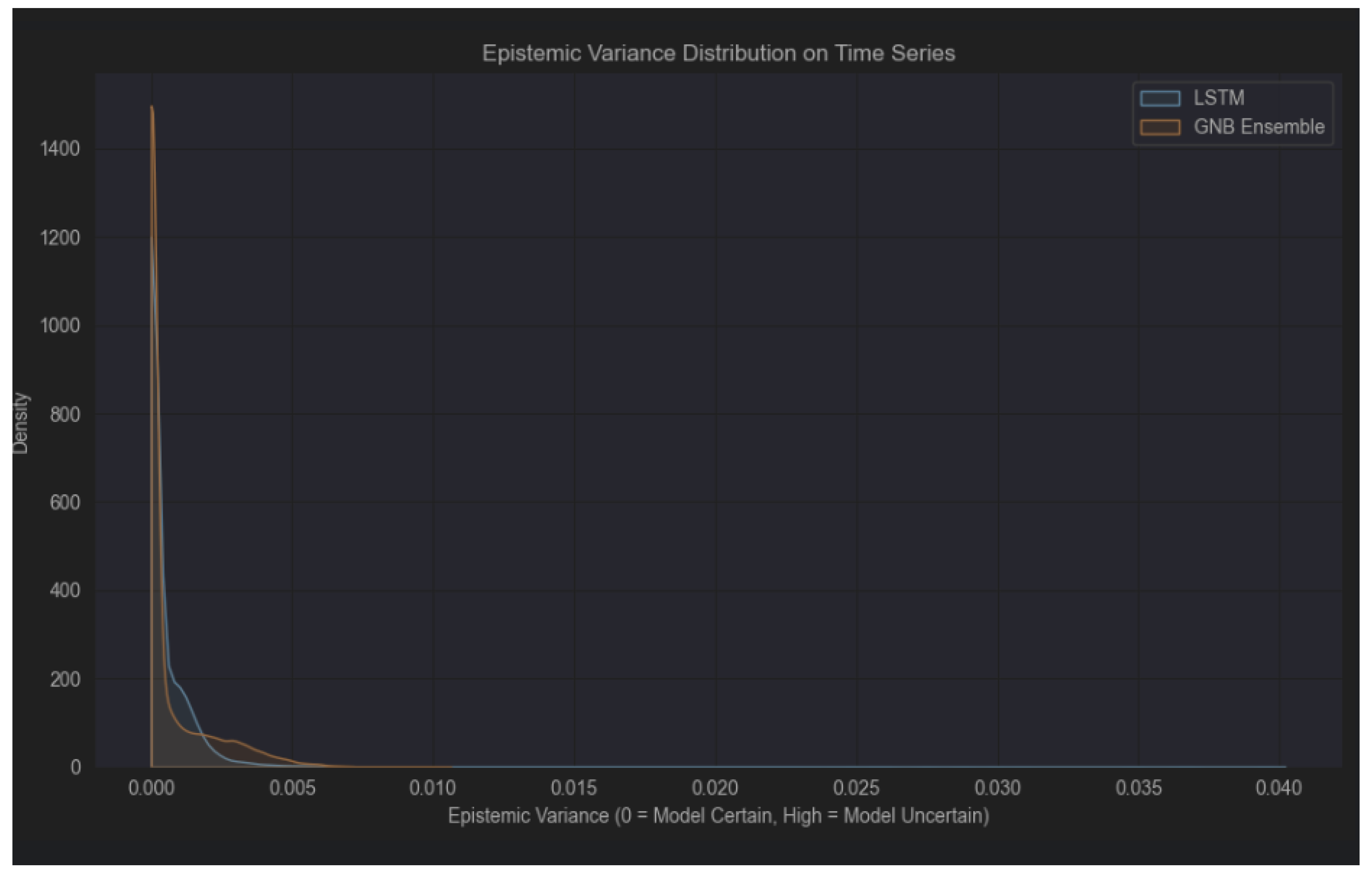
Figure 11.
Epistemic variance distribution (KDE) on the time series test set for LSTM (MC Dropout) and GNB Window Ensemble. GNB Window is deterministic and therefore excluded. Both distributions are strongly concentrated near zero, confirming that model-level uncertainty is low for the majority of test windows. The GNB Ensemble exhibits a heavier tail extending to ≈ 0.040, whereas the LSTM variance decays more rapidly, suggesting that MC Dropout produces tighter and more consistent epistemic uncertainty estimates than bootstrap ensembling on this dataset.
Figure 11.
Epistemic variance distribution (KDE) on the time series test set for LSTM (MC Dropout) and GNB Window Ensemble. GNB Window is deterministic and therefore excluded. Both distributions are strongly concentrated near zero, confirming that model-level uncertainty is low for the majority of test windows. The GNB Ensemble exhibits a heavier tail extending to ≈ 0.040, whereas the LSTM variance decays more rapidly, suggesting that MC Dropout produces tighter and more consistent epistemic uncertainty estimates than bootstrap ensembling on this dataset.
5.3. Cross-Experiment Comparison of Uncertainty Strategies
Table 4 summarises the best model for each uncertainty strategy along two axes: calibration quality (ECE) and error detection utility (AUC).
The MC Dropout strategy achieves the optimal combination of accuracy, calibration, and error detection, although this result is observed on a substantially larger time series dataset (22 372 vs. 56 test samples) and is therefore not directly comparable to the feature-set results. Among the feature-set strategies, Bayesian MCMC provides the best calibration (ECE = 0.060), while tree-level variance (Random Forest) achieves the highest error detection utility (AUC = 0.909), followed closely by bootstrap ensembling (GNB Ensemble, AUC = 0.855).
Figure 12.
MC Dropout convergence diagnostics for the LSTM model. Each panel shows how accuracy, mean predictive entropy, and mean epistemic variance evolve as the number of stochastic forward passes T increases from 5 to 100. All three statistics stabilise well before , confirming that the Monte Carlo estimator has converged.
Figure 12.
MC Dropout convergence diagnostics for the LSTM model. Each panel shows how accuracy, mean predictive entropy, and mean epistemic variance evolve as the number of stochastic forward passes T increases from 5 to 100. All three statistics stabilise well before , confirming that the Monte Carlo estimator has converged.
6. Discussion
6.1. Calibration vs. Accuracy Trade-Off
The most striking finding of this study is the inverse relationship between point accuracy and calibration quality observed on the feature set. The highest-accuracy model — Random Forest (89.5%) — ranks last in ECE (0.166), while XGBoost and QDA, despite achieving accuracies of 86.8% and 87.5% respectively, also exhibit relatively poor calibration (ECE of 0.093 and 0.103). By contrast, the best-calibrated model (Bayesian Softmax, ECE = 0.060) achieves an intermediate accuracy of 88.8%. This observation is consistent with the overconfidence phenomenon widely described in the literature [6,7,8]: discriminative classifiers trained to maximise accuracy tend to sharpen their probability outputs, producing overconfident predictions that inflate ECE.
The Bayesian Softmax model avoids this pitfall by maintaining a full posterior distribution over parameters. Rather than fitting a single weight vector that maximises training likelihood, MCMC sampling explores the space of plausible parameterisations. This ensemble of explanations naturally hedges confident predictions, producing softer probability outputs that more accurately reflect the true classification uncertainty.
6.2. Bootstrap Ensemble as a Universal Uncertainty Improver
A practical recommendation emerging from this study is that bootstrap ensembling should be applied as a standard post-hoc augmentation for any classifier used in safety-critical fault diagnosis. The improvement is most dramatic for models with intrinsically poor uncertainty quantification: XGBoost’s NLL fell from 0.357 to 0.314 and ECE from 0.093 to 0.088 with just 20 bootstrap replicates, while GNB’s NLL improved from 0.564 to 0.413 with 50 replicates.
However, the QDA Ensemble case illustrates that bootstrap ensembling is not universally beneficial. QDA estimates full covariance matrices for each class, and on a small dataset (128 training samples, 32 per class), bootstrap resampling produces replicates with significantly varied covariance estimates. The resulting ensemble average can have worse calibration than a single model trained on all available data (ECE rising from 0.103 to 0.108). This suggests that the effectiveness of bootstrap ensembling depends on the stability of the base classifier with respect to training set perturbations.
6.3. Monte Carlo Dropout — Best of Both Worlds
LSTM with MC Dropout represents the ideal scenario in our experiments: simultaneously the highest accuracy (95.0%) and the best calibration (ECE = 0.015), with the highest Error Detection AUC (0.946). This success can be attributed to three factors: (a) the larger time series dataset (124 644 training windows) provides sufficient data for the LSTM to learn accurate representations; (b) dropout regularisation during training prevents overfitting, maintaining well-calibrated probabilities; and (c) MC Dropout at inference provides multiple stochastic predictions whose variance directly estimates epistemic uncertainty [10].
The practical implication is that for applications with sufficient time series data, LSTM with MC Dropout provides a compelling single-model solution that does not require separate calibration or ensemble infrastructure.
6.4. Practical Implications for Industrial Deployment
Based on the results, we recommend a layered deployment strategy for motor fault diagnosis systems:
Primary classifier. A high-accuracy model (Random Forest or QDA) for the classification decision.
Uncertainty gating. A parallel Bayesian Softmax or bootstrap ensemble model whose uncertainty estimate determines the action: below a threshold — the primary classifier’s decision is executed; above the threshold — the sample is flagged for human review. This approach is consistent with the concept of classification with rejection [4], in which rejecting uncertain predictions and routing them to a human expert significantly reduces the number of misclassifications while making the system more trustworthy.
When sufficient time series data are available, LSTM with MC Dropout can serve both roles simultaneously, providing high accuracy and well-calibrated uncertainty in a single inference pipeline.
6.5. Limitations
The feature-set experiment operates on only 56 test samples, limiting the statistical significance of metric differences and precluding the computation of confidence intervals on ECE and AUC estimates. The time series experiment, with 22 372 test windows, provides more robust estimates but compares fewer model configurations. Furthermore, this study evaluates uncertainty exclusively on in-distribution data; assessing model behaviour on OOD data — e.g., using dataset dissimilarity measures [15] — constitutes an important direction for future work. Further extensions should include bootstrapped confidence intervals on all uncertainty metrics as well as additional architectures (e.g., convolutional networks, attention-based models).
7. Conclusions
In this work, which constitutes a continuation of the classification research presented in [1], pre-trained probabilistic prediction models were applied to motor state classification, and the quality of their predictive uncertainty was subsequently modelled and compared. Five distinct uncertainty extraction strategies — native probabilistic outputs, Random Forest tree-level variance, bootstrap ensemble aggregation, Bayesian MCMC posterior sampling, and Monte Carlo Dropout — were evaluated using six quantitative metrics on two complementary data representations. The main findings are as follows: (1) Bayesian Softmax Regression achieves the best calibration (ECE = 0.060) on the statistical feature set, confirming that principled posterior inference produces more reliable confidence estimates than discriminative optimisers, even at the cost of lower point accuracy. (2) Bootstrap ensemble augmentation is a widely accessible method that improves uncertainty quality for most classifiers; however, the highest Error Detection AUC on the feature set (0.909) was achieved by Random Forest, which combines strong discriminative performance with natural epistemic variance from tree-level disagreement. (3) LSTM with MC Dropout delivers the strongest overall performance on the time series set, simultaneously achieving the highest accuracy (95.0%), best calibration (ECE = 0.015), and highest Error Detection AUC (0.946). (4) Overconfidence poses a real threat: single XGBoost, despite 94.6% accuracy, has a near-random Error Detection AUC (0.535), making it unreliable for flagging errors without additional uncertainty infrastructure. These results provide practical guidance for practitioners deploying diagnostic systems in safety-critical industrial environments, where reliable uncertainty quantification is not merely desirable but essential.
Author Contributions
Conceptualisation, methodology, software, formal analysis, investigation, data curation, writing—original draft, writing—review and editing, and visualisation were performed by N.S. and J.T. Supervision was provided by W.B. All authors have read and agreed to the published version of the manuscript.
Funding
This research received no external funding.
Institutional Review Board Statement
Not applicable.
Informed Consent Statement
Not applicable.
Data Availability Statement
The datasets, evaluation module code (UncertaintyEvaluator, BootstrapEnsemble), and trained model artefacts used in this study are available from the corresponding author upon reasonable request.
Conflicts of Interest
The authors declare no conflicts of interest.
Abbreviations
The following abbreviations are used in this manuscript:
| AUC | Area Under the ROC Curve |
| BNN | Bayesian Neural Network |
| BS | Brier Score |
| ECE | Expected Calibration Error |
| GNB | Gaussian Naive Bayes |
| LSTM | Long Short-Term Memory |
| MC | Monte Carlo |
| MCMC | Markov Chain Monte Carlo |
| NLL | Negative Log-Likelihood |
| NUTS | No-U-Turn Sampler |
| OOD | Out-of-Distribution |
| QDA | Quadratic Discriminant Analysis |
| RF | Random Forest |
| ROC | Receiver Operating Characteristic |
| UQ | Uncertainty Quantification |
References
- Tomczyk, J.; Szewczak, N.; Bauer, W. Statistical models for fault detection in mechanical devices. Automation 2026, submitted.
- Baranowski, J.; Bauer, W.; Jarzyna, K.; Piątek, P. DUDU-BLDC: Data set for diagnostic of Brushless DC motors with degrading magnets. Zenodo 2025. [Google Scholar] [CrossRef]
- Koblinger, Á.; Fiser, J.; Lengyel, M. Representations of uncertainty: where art thou? Curr. Opin. Behav. Sci. 2021, 38, 150–162. [Google Scholar] [CrossRef]
- Thuy, A.; Benoit, D.F. Explainability through uncertainty: Trustworthy decision-making with neural networks. Eur. J. Oper. Res. 2024, 317(2), 330–340. [Google Scholar] [CrossRef]
- Wang, C.; Chen, X.; Qiang, X.; Fan, H.; Li, S. Recent advances in mechanism/data-driven fault diagnosis of complex engineering systems with uncertainties. AIMS Math. 2024, 9(11), 29736–29772. [Google Scholar] [CrossRef]
- Guo, C.; Pleiss, G.; Sun, Y.; Weinberger, K.Q. On calibration of modern neural networks. In Proceedings of the 34th International Conference on Machine Learning (ICML), Sydney, Australia, 6–11 August 2017; pp. 1321–1330. [Google Scholar]
- Fakour, F.; Mosleh, A.; Ramezani, R. A Structured Review of Literature on Uncertainty in Machine Learning & Deep Learning. arXiv 2024, arXiv:2406.00332. [Google Scholar]
- Weytjens, H.; Verbeke, W. Uncertainty in Machine Learning. In AI for Business: From Data to Decisions; 2025. [Google Scholar]
- Hüllermeier, E.; Waegeman, W. Aleatoric and epistemic uncertainty in machine learning: an introduction to concepts and methods. Mach. Learn. 2021, 110(3), 457–506. [Google Scholar] [CrossRef]
- Gal, Y.; Ghahramani, Z. Dropout as a Bayesian approximation: Representing model uncertainty in deep learning. In Proceedings of the 33rd International Conference on Machine Learning (ICML), New York, NY, USA, 20–22 June 2016; pp. 1050–1059. [Google Scholar]
- Lakshminarayanan, B.; Pritzel, A.; Blundell, C. Simple and scalable predictive uncertainty estimation using deep ensembles. In Advances in Neural Information Processing Systems; Curran Associates: Long Beach, CA, USA, 2017; Volume 30, pp. 6402–6413. [Google Scholar]
- Lakshminarayanan, B. Introduction to Uncertainty in Deep Learning. Presentation at the CIFAR Deep Learning and Reinforcement Learning Summer School, 2020. [Google Scholar]
- Jospin, L.V.; Laga, H.; Boussaid, F.; Buntine, W.; Bennamoun, M. Hands-on Bayesian neural networks—a tutorial for deep learning users. IEEE Comput. Intell. Mag. 2022, 17(2), 29–48. [Google Scholar] [CrossRef]
- Efron, B.; Tibshirani, R.J. An Introduction to the Bootstrap; CRC Press: Boca Raton, FL, USA, 1994. [Google Scholar]
- Incorvaia, G.; Hond, D.; Asgari, H. Uncertainty Quantification of Machine Learning Model Performance via Anomaly-Based Dataset Dissimilarity Measures. Electronics 2024, 13(5), 939. [Google Scholar] [CrossRef]
- Han, T.; Li, Y.-F. Out-of-distribution detection-assisted trustworthy machinery fault diagnosis approach with uncertainty-aware deep ensembles. Reliab. Eng. Syst. Saf. 2022, 226, 108648. [Google Scholar] [CrossRef]
- Jalayer, R.; et al. Evaluating deep learning models for fault diagnosis of a rotating machinery with epistemic and aleatoric uncertainty. arXiv 2024, arXiv:2412.18980. [Google Scholar]
- Chen, L.; et al. Trustworthy Bayesian deep learning framework for uncertainty quantification and confidence calibration: Application in machinery fault diagnosis. Reliab. Eng. Syst. Saf. 2024. [Google Scholar] [CrossRef]
- Hoffman, M.D.; Gelman, A. The No-U-Turn Sampler: Adaptively setting path lengths in Hamiltonian Monte Carlo. J. Mach. Learn. Res. 2014, 15, 1593–1623. [Google Scholar]
- Abril-Pla, O.; et al. PyMC: A modern and comprehensive probabilistic programming framework in Python. PeerJ Comput. Sci. 2023, 9, e1516. [Google Scholar] [CrossRef]
- Brier, G.W. Verification of forecasts expressed in terms of probability. Mon. Weather Rev. 1950, 78(1), 1–3. [Google Scholar]
- Naeini, M.P.; Cooper, G.F.; Hauskrecht, M. Obtaining well calibrated probabilities using Bayesian binning. In Proceedings of the 29th AAAI Conference on Artificial Intelligence, Austin, TX, USA, 25–30 January 2015; pp. 2901–2907. [Google Scholar]
- Kendall, A.; Gal, Y. What uncertainties do we need in Bayesian deep learning for computer vision? In Advances in Neural Information Processing Systems; Curran Associates: Long Beach, CA, USA, 2017; Volume 30, pp. 5574–5584. [Google Scholar]

Table 1.
Models and uncertainty quantification strategies evaluated in each experiment.
| Model | UQ Strategy | Dataset |
|---|---|---|
| Random Forest (single) | Tree-level variance | Feature set |
| XGBoost (single) | Native softmax | Feature set |
| XGBoost Ensemble () | Bootstrap aggregation | Feature set |
| Gaussian NB (single) | Native posterior | Feature set |
| GNB Ensemble () | Bootstrap aggregation | Feature set |
| QDA (single) | Native posterior | Feature set |
| QDA Ensemble () | Bootstrap aggregation | Feature set |
| Bayesian Softmax | MCMC posterior () | Feature set |
| LSTM (MC Dropout, ) | MC Dropout | Time series |
| GNB Window Ensemble () | Bootstrap (flattened) | Time series |
| GNB Window (single) | Native posterior | Time series |
Table 2.
Uncertainty metrics on the statistical feature test set (). Values reported as mean ± std from Repeated Stratified K-Fold ( folds); Bayesian Softmax from posterior subsampling (10 subsets × 400 samples). ↓ — lower is better; ↑ — higher is better. Best values per metric are shown in bold.
Table 2.
Uncertainty metrics on the statistical feature test set (). Values reported as mean ± std from Repeated Stratified K-Fold ( folds); Bayesian Softmax from posterior subsampling (10 subsets × 400 samples). ↓ — lower is better; ↑ — higher is better. Best values per metric are shown in bold.
| Model | Acc. ↑ | NLL ↓ | Brier ↓ | ECE ↓ | Entropy | Epist. Var. |
|---|---|---|---|---|---|---|
| Random Forest | ||||||
| XGBoost | — | |||||
| XGBoost Ens. | ||||||
| Gaussian NB | — | |||||
| GNB Ensemble | ||||||
| QDA | — | |||||
| QDA Ensemble | ||||||
| Bayesian Softmax |
Table 3.
Uncertainty metrics on the time window test set (). Values reported as mean ± std: LSTM from 5 independent MC sampling rounds, GNB models from Repeated Stratified K-Fold ( folds). Notation as in Table 2.
Table 3.
Uncertainty metrics on the time window test set (). Values reported as mean ± std: LSTM from 5 independent MC sampling rounds, GNB models from Repeated Stratified K-Fold ( folds). Notation as in Table 2.
| Model | Acc. ↑ | NLL ↓ | Brier ↓ | ECE ↓ | Entropy | Epist. Var. |
|---|---|---|---|---|---|---|
| LSTM (MC Dropout) | ||||||
| GNB Window Ens. | ||||||
| GNB Window | — |
Table 4.
Summary: best model per UQ strategy.
| Strategy | Best Model | Accuracy | ECE | Error Det. AUC |
|---|---|---|---|---|
| Native softmax | QDA | 0.875 | 0.103 | — |
| Tree-level var. | Random Forest | 0.895 | 0.166 | 0.909 |
| Bootstrap ensemble | GNB Ensemble | 0.882 | 0.105 | 0.855 |
| Bayesian MCMC | Bayesian Softmax | 0.888 | 0.060 | 0.817 |
| MC Dropout | LSTM | 0.950 | 0.015 | 0.945 |
Disclaimer/Publisher’s Note: The statements, opinions and data contained in all publications are solely those of the individual author(s) and contributor(s) and not of MDPI and/or the editor(s). MDPI and/or the editor(s) disclaim responsibility for any injury to people or property resulting from any ideas, methods, instructions or products referred to in the content. |
© 2026 by the authors. Licensee MDPI, Basel, Switzerland. This article is an open access article distributed under the terms and conditions of the Creative Commons Attribution (CC BY) license (http://creativecommons.org/licenses/by/4.0/).
Copyright: This open access article is published under a Creative Commons CC BY 4.0 license, which permit the free download, distribution, and reuse, provided that the author and preprint are cited in any reuse.