
Submitted:
15 September 2026
Posted:
15 September 2026
You are already at the latest version
Abstract
The reliability of traction-motor winding insulation directly affects the safe operation of electric vehicles. This study proposes a remaining-useful-life (RUL) prediction method for traction-motor main insulation using bipolar-pulse response measurements and Gaussian process regression (GPR). Simulated winding modules were subjected to full-lifecycle accelerated thermal aging at 300 °C. During the diagnostic stage of each aging subcycle, bipolar high-voltage pulses were applied, and synchronized insulation-voltage and insulation-current waveforms were acquired at 50 MSPS. A 2 μs oscillatory segment associated with the positive-polarity rising edge was processed using a Hann window, a 10th-order Butterworth band-pass filter from 2 to 12 MHz, and a 100-point fast Fourier transform. The frequency bin with the maximum current-spectrum magnitude was identified, and the impedance magnitude was calculated from the voltage-to-current spectral-magnitude ratio at the same frequency. The impedance magnitude was then multiplied by the corresponding frequency to obtain a frequency-weighted impedance feature. The feature was corrected to a reference temperature of 85 °C. One complete lifetime trajectory containing 119 diagnostic measurements was used for proof-of-concept evaluation. The initial feature was 13.7076 Ω·MHz, and the end-of-life threshold was defined as twice this value, 27.4152 Ω·MHz. The first threshold crossing occurred at 428.405 h. A trend-informed GPR model combining causal averaging, monotonic trend extraction, a quadratic mean function, and a short-memory Matérn-3/2 residual process was updated after each new measurement. Across ten rolling prediction origins after 80% of the observed lifetime, all ten origins produced finite threshold-crossing-based RUL estimates. The mean bounded relative accuracy was 80.08%, with an MAE of 6.455 h and an RMSE of 8.923 h. The results demonstrate the feasibility of waveform-feature-based chronological RUL prediction, while independent multi-specimen validation remains necessary.
Keywords:
electric vehicle
; traction motor
; winding insulation
; accelerated thermal aging
; bipolar high-voltage pulse
; frequency-weighted impedance
; Gaussian process regression
; remaining useful life
1. Introduction
Electrified powertrains are moving toward higher dc-link voltages, faster wide-bandgap switching devices, and increased power density [1,2]. These developments improve system efficiency and reduce mass, but they also increase the electrical stress imposed on traction-motor windings. Fast voltage edges, cable–motor impedance mismatch, reflected waves, and winding resonances can produce terminal overvoltage, nonlinear turn-voltage distribution, and high-frequency oscillation. Consequently, winding insulation is exposed to repetitive pulses whose amplitude, rise time, repetition rate, and polarity-reversal characteristics can be substantially more severe than those associated with conventional sinusoidal excitation [3,4,5,6,7,8,9].
The electrical insulation system is a principal reliability bottleneck in high-utilization electrical machines. Its degradation is governed by interacting thermal, electrical, ambient, and mechanical stresses. In inverter-fed traction motors, repetitive voltage pulses, partial-discharge activity, dielectric heating, charge accumulation, and repetitive-impulse effects can accelerate insulation deterioration [10,11,12,13,14]. Accelerated lifetime testing, condition monitoring, and degradation-sensitive electrical measurements have therefore received increasing attention as means of identifying insulation deterioration before final breakdown [15,16,17,18]. IEC standards provide qualification and functional-evaluation procedures for converter-fed and wire-wound rotating-machine insulation systems [19,20,21]. However, these procedures are primarily intended for insulation-system qualification and thermal classification rather than online or periodically updated remaining-useful-life prediction.
Traditional lifetime assessment commonly employs physics-based thermal or electrothermal models fitted to breakdown-time data. Such models are valuable for insulation design and qualification, but they require an assumed degradation relationship and may not fully exploit information contained in measured transient waveforms. Conversely, condition indicators such as capacitance, dissipation factor, partial-discharge inception voltage, insulation resistance, leakage current, and transient-current response can reflect progressive changes in dielectric properties. Current-response-based identification has demonstrated that insulation degradation can be detected from the transient response following an applied voltage step [15]. High-voltage rectangular-pulse generators have also been developed to reproduce fast repetitive electrical stresses and evaluate inverter-fed motor insulation [22]. These studies motivate the synchronous acquisition of complete high-frequency voltage and insulation-current waveforms and the extraction of degradation-sensitive spectral features from their transient responses.
Data-driven prognostics provide a means of mapping degradation indicators to lifetime without requiring a complete microscale degradation model. Gaussian process regression (GPR) is attractive for accelerated-aging data because it offers flexible nonlinear regression, is applicable to small-to-moderate datasets, and can represent correlated residual behavior through a covariance kernel [23]. Bayesian prognostics and GPR-based remaining-life studies in other degradation systems have further demonstrated the value of chronological health-indicator forecasting when complete run-to-failure samples are limited [24,25,26]. In the present study, GPR is used to model the short-memory residual around a physically constrained degradation trend. The model forecasts the future trajectory of a waveform-derived insulation feature, while the end-of-life time and remaining useful life (RUL) are inferred from the first crossing of a fixed feature threshold.
This study develops a waveform-feature-based RUL prediction framework for the main insulation of simulated electric-vehicle traction-motor winding modules. The main contributions are as follows: (1) a customized constant-temperature, full-lifecycle accelerated-aging procedure combined with periodic bipolar high-voltage pulse interrogation; (2) a synchronized high-frequency waveform-processing method that identifies the frequency bin with the maximum current-spectrum magnitude and constructs a temperature-corrected, frequency-weighted impedance feature from the voltage and current spectral magnitudes at the same frequency; (3) a trend-informed GPR method combining seven-point causal averaging, isotonic degradation-trend extraction, a nondecreasing quadratic mean function, and a short-memory Matérn-3/2 residual process; and (4) a chronological rolling-origin evaluation using one complete lifetime trajectory containing 119 diagnostic measurements. For ten prediction origins after 80% of the observed lifetime, the proposed method achieved a mean bounded relative RUL accuracy of 80.08%, with a mean absolute error of 6.455 h and a root-mean-square error of 8.923 h. Because only one complete lifetime trajectory was used, the reported performance is interpreted as a proof-of-concept result rather than independent specimen-level validation.
2. Accelerated Aging Experiment and Pulse-Response Measurement
2.1. Simulated Winding-Module Specimens
The test objects were simulated winding modules designed to reproduce the main-insulation structure of a traction motor. The configuration and physical prototype of the specimen are shown in Figure 1.
Each module consisted of a laminated stator-core segment with two slots and three teeth and an axial core length of 135 mm. The winding was installed in the two slots to form a closed coil around the central tooth, providing a representative conductor-to-ground insulation path between the energized winding and the grounded stator core.
Each coil comprised 15 turns, with nine round copper conductors connected in parallel in each turn. The conductor diameter was 0.8 mm, and H-class enameled wire with a thermal rating of 180 °C was used. After winding and slot assembly, the specimens were vacuum impregnated with an H-class insulating varnish to consolidate the winding and reproduce the impregnation condition of traction-motor insulation.
The core geometry, winding arrangement, conductor specification, and impregnation process were kept consistent across all specimens. This controlled configuration reduced specimen-to-specimen variation and enabled changes in the measured electrical response to be attributed primarily to insulation aging. Before the accelerated aging experiment, each specimen was visually inspected and subjected to an initial electrical test. The resulting measurements were used as the unaged baseline for subsequent full-lifecycle comparisons.
Two nominally identical specimens were included in the accelerated-aging experiment to provide experimental redundancy and reduce the risk that accidental specimen damage during the prolonged aging process would prevent acquisition of a complete lifetime trajectory. The lifetime-prediction analysis presented in this study was based on the complete full-lifecycle dataset obtained from one specimen, comprising 119 diagnostic measurements over an observed lifetime of 428.405 h. The second specimen served as an experimental backup and was not included in the GPR modeling dataset.
2.2. Full-Lifecycle Constant-Temperature Aging Test
A full-lifecycle accelerated thermal-aging experiment was conducted to characterize the progressive degradation of the winding-insulation specimens from the unaged state to final failure. The experimental procedure was developed with reference to IEC 60034-18-21 and customized according to the practical requirements of accelerated lifetime testing for motor-winding insulation [21]. On this basis, periodic bipolar high-voltage pulse measurements were incorporated into the aging procedure to acquire electrical-response waveforms at different stages of insulation degradation.
The specimens were installed in a constant-temperature aging chamber and aged at 300 °C according to the predefined procedure. This elevated temperature was selected to produce observable insulation degradation within a manageable experimental duration. The specimen arrangement and chamber-temperature setting were maintained consistently throughout the experiment.
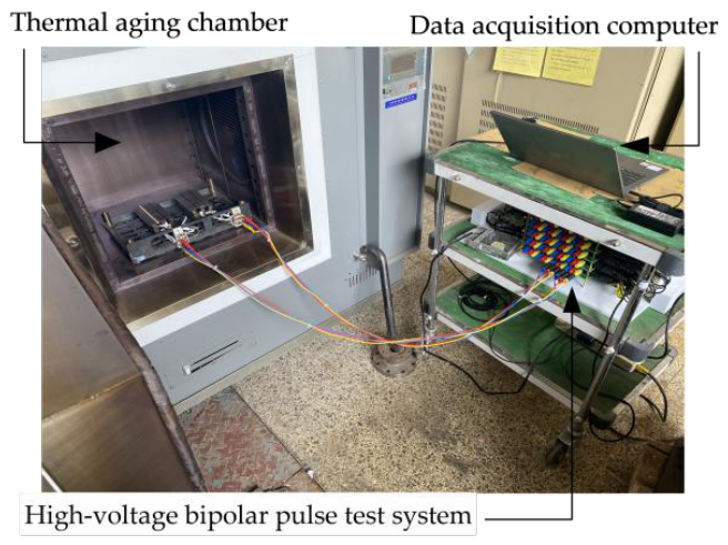
Figure 2.
Experimental setup for the full-lifecycle constant-temperature accelerated aging test.
The complete experiment consisted of a series of aging–measurement subcycles, as illustrated in Figure 3. Before accelerated aging, each specimen was visually inspected and subjected to an initial electrical measurement to establish its unaged baseline. During each subcycle, the specimens were exposed to the constant aging temperature for a specified period. Aging was then temporarily interrupted, and the specimens were tested according to the predefined bipolar high-voltage pulse measurement procedure. The high-frequency voltage and insulation-current waveforms obtained at each inspection point were synchronously recorded. After the measurement was completed, the specimens were returned to the aging chamber to begin the next subcycle.
The average duration of an aging subcycle was approximately 4.3 h. However, because of operational interruptions, specimen inspections, equipment adjustments, and other uncertainties during the experiment, the actual duration of an individual subcycle varied from 0.6 to 24.2 h. The duration of every subcycle was recorded in detail. Consequently, cumulative aging time, rather than the number of completed subcycles, was used as the experimental time coordinate in the subsequent degradation-feature analysis and lifetime-prediction model. For the k-th measurement point, the cumulative aging time was calculated as
where Δtj denotes the recorded duration of the j-th aging subcycle. This treatment accounts for the unequal time intervals between successive measurements and prevents variations in subcycle duration from introducing systematic errors into the lifetime analysis.
The aging–measurement procedure was repeated until the corresponding specimen reached the predefined end-of-life condition. The cumulative aging time at failure was recorded as the experimental lifetime of that specimen. The same pulse-measurement configuration, wiring arrangement, and instrument settings were maintained as far as practicable at each inspection point so that changes in the acquired voltage and current waveforms primarily reflected the progressive degradation of the winding insulation.
Representative specimen states at different stages of the experiment are shown in Figure 4. The unaged specimens exhibited intact winding surfaces and insulation structures. As the cumulative aging time increased, visible discoloration and material deterioration gradually appeared. After failure, severe darkening and localized damage could be observed. These visual changes provided qualitative evidence of progressive thermal degradation and supported the subsequent analysis of waveform-derived aging features.
2.3. Bipolar High-Voltage Pulse Test Platform
A dedicated bipolar high-voltage pulse test platform was developed to periodically characterize the main-insulation condition of the winding-module specimens during accelerated aging. The system architecture is shown in Figure 5.
The platform mainly comprised a high-voltage power supply, a low-voltage auxiliary power supply, an H-bridge pulse-generation circuit, a gate-driver board, multi-channel switching units, interface-protection units, high-frequency voltage and leakage-current sensors, a temperature-sensing unit, and a control and data-acquisition unit. These functional modules were integrated into a compact platform capable of automatically applying bipolar voltage pulses and acquiring the corresponding electrical responses from multiple specimens.
The high-voltage source was an HSPY-1500-002 power supply rated at 1500 V/200 mA. The H-bridge converted the DC output into bipolar voltage pulses under the control of the gate-driver board. An LRS-100-12 low-voltage power supply rated at 12 V/8.5 A supplied the control, sensing, switching, and driver circuits through several DC/DC conversion stages. The multi-channel switching units selected the specimen and measurement path according to commands issued by the control unit, while the interface-protection units provided electrical isolation and protected the sensing and acquisition circuits against transient overvoltage.
The electrical connection between the pulse-generation circuit, the insulation specimen, and the sensing units is illustrated in Figure 6. During measurement, the two winding terminals were connected to the bipolar-pulse output, and the stator core was connected to the reference-ground path. A high-frequency voltage sensor unit (HFHSVT) measured the voltage applied across the winding-to-core insulation. Meanwhile, a high-frequency, high-sensitivity leakage-current sensor unit (HFHSCT) measured the insulation current flowing through the conductor-to-ground path. A high-sensitivity temperature sensor unit (HSTT) was used to monitor the specimen temperature during the diagnostic procedure.
The core control and data-acquisition unit was implemented using a Xilinx Zynq-7000 XC7Z020 system-on-chip (SoC), which integrates a dual-core ARM processor and field-programmable gate array (FPGA) resources on a single device. The FPGA was responsible for deterministic pulse-control timing, specimen-channel switching, and high-speed acquisition of the voltage and insulation-current signals. The ARM processing system performed system configuration, acquisition-process management, data organization, and communication with the host computer.
An AD9226-based high-speed analog-to-digital converter (ADC) front end was used to digitize the outputs of the voltage and leakage-current sensors. The voltage and insulation-current channels were sampled synchronously at 50 MSPS, enabling the applied pulse voltage and its corresponding current response to be recorded using a common time reference. The digitized waveform data were transferred directly to the Zynq-based acquisition unit and subsequently transmitted to the host computer for storage and feature extraction. Therefore, the measurement process was completed by the dedicated embedded acquisition system without using an external oscilloscope.
The three-dimensional layout, functional-module arrangement, and physical prototype of the developed Zynq-based bipolar high-voltage pulse test platform are presented in Figure 7.
At each aging state, the specimen was excited using the same predefined bipolar-pulse sequence. Bipolar excitation was used as a repeatable diagnostic perturbation to generate switching transients of both polarities. At a repetition frequency of 0.1 Hz, the pulse sequence was not intended to reproduce the switching frequency or cumulative electrical-aging stress of an operating traction inverter [3,10,12]; rather, it served to interrogate the insulation response periodically during the thermal-aging experiment. To ensure comparability among different aging states, the pulse parameters, specimen connections, channel-selection procedure, sensor configuration, and acquisition settings were maintained consistently throughout the experiment.
Before each measurement, the specimen channel and electrical connections were checked to avoid poor contact or incorrect grounding. The acquired signals were examined for channel-switching errors, sensor saturation, and abnormal interference. Only valid voltage and insulation-current waveforms were retained for subsequent analysis. This dedicated measurement platform provided repeatable full-lifecycle waveform data without relying on an external oscilloscope and established the experimental basis for extracting aging-sensitive features.
2.4. Voltage and Current Waveform Acquisition
At each scheduled measurement point, the bipolar-pulse voltage v(t) applied to the winding insulation and the corresponding insulation current i(t) were acquired synchronously using the dedicated Zynq-based control and data-acquisition unit. The voltage and current sensor outputs were digitized by the AD9226-based analog-to-digital conversion front end. Both channels operated at a sampling rate of 50 MSPS, corresponding to a sampling interval of 20 ns. The synchronous dual-channel configuration ensured that the applied voltage and its associated current response were recorded using the same time reference.
The FPGA resources of the Zynq XC7Z020 SoC controlled the acquisition timing and generated a common trigger synchronized with the bipolar-pulse sequence. Following the trigger event, the voltage and current samples were acquired in parallel and temporarily buffered in the programmable logic. The sampled data were subsequently transferred to the dual-core ARM processing system, organized into paired voltage–current waveform records, and transmitted to the host computer for storage. Each waveform record was associated with the specimen identifier, measurement sequence, and cumulative aging time, allowing the electrical response of each specimen to be traced throughout the accelerated aging experiment.
The same sensor configuration, sampling rate, trigger position, channel gain, and acquisition window were maintained at different aging states. Before storage, the acquired records were checked for incomplete data, abnormal channel switching, analog-to-digital converter saturation, and evident external interference. The original sampled waveforms were retained without feature-level compression to preserve the short-duration peaks and high-frequency oscillatory components associated with pulse switching.
Figure 8 confirms that the 60 μs acquisition window captured all four principal switching transitions without evident channel clipping. The subsequent feature-extraction procedure used only the synchronized response following the positive-polarity rising edge, whereas the complete waveform record was retained for traceability.
Figure 8 shows a representative voltage–current record over a 60 μs observation window. The voltage waveform contains a positive pulse plateau of approximately +0.5 kV and a negative pulse plateau of approximately -0.5 kV, each with a pulse width of approximately 10 μs. Short-duration voltage overshoots occur at the rising and falling edges because of the high switching speed and the distributed inductive and capacitive parameters of the pulse-generation circuit, connecting cables, sensors, and test specimen.
The insulation-current waveform is concentrated primarily around the four voltage transitions. Each switching edge produces a large transient-current peak followed by a damped oscillatory response. Compared with the relatively stable voltage plateaus, the current waveform exhibits more pronounced changes in amplitude, decay rate, oscillation frequency, and waveform shape. These characteristics are affected by the effective capacitance, dielectric polarization, leakage conduction, and high-frequency equivalent impedance of the winding-to-ground insulation path. Although the complete 60 μs voltage–current waveform was acquired and retained, only the 2 μs oscillatory response associated with the positive-polarity rising edge was selected for subsequent feature extraction and insulation-lifetime prediction, as described in Section 3.1.
2.5. Failure Criterion and Lifetime Definition
The accelerated aging–measurement procedure was continued until each winding-module specimen reached the predefined end-of-life condition. Two diagnostic quantities were used to evaluate insulation failure: winding-to-ground capacitance and insulation resistance. For specimen i, the initial winding-to-ground capacitance measured before accelerated aging was denoted by Ci,0. At the j-th inspection point, the corresponding capacitance and insulation resistance were denoted by Ci,j and Ri,j, respectively.
A specimen was considered to have reached the end of life when either of the following conditions was satisfied:
or
The capacitance criterion represents a substantial change in the effective dielectric and structural characteristics of the winding-to-ground insulation path, whereas the insulation-resistance criterion identifies a severe deterioration in its ability to suppress conductive leakage. Using the logical “OR” relationship ensured that either type of significant insulation degradation could trigger the end-of-life decision.
Because the duration of the aging subcycles was not constant, specimen lifetime was determined using the recorded cumulative aging time rather than the number of completed subcycles. For specimen i, the experimentally observed lifetime Li was defined as
where Δti,k is the recorded duration of the k-th aging subcycle and Ki is the first subcycle at which either end-of-life criterion was satisfied. Thus, Li represents the cumulative aging time from the beginning of the experiment to the first confirmed end-of-life event.
For the specimen used in the lifetime-prediction analysis, the EOL at 428.405 h was independently confirmed according to the predefined logical-OR criterion, under which satisfaction of either the capacitance criterion or the insulation-resistance criterion indicated EOL. At this diagnostic point, the winding-to-ground capacitance measured at 10 kHz was 104 pF, corresponding to 44.6% of its initial value and therefore satisfying the capacitance criterion. Meanwhile, the insulation resistance measured at 500 V remained above 550 MΩ and did not satisfy the insulation-resistance criterion. Both measurements were performed at a specimen temperature of 25 °C. The waveform-feature threshold described in Section 3 was derived from the predefined capacitance criterion and fixed before the rolling prediction analysis; it was not used to define the experimentally observed EOL.
For retrospective evaluation of the lifetime-prediction results, the actual remaining useful life at the j-th diagnostic measurement of specimen i was calculated as
where is the cumulative aging time at the corresponding measurement point. This value was calculated only after the experimentally observed lifetime had been determined and was used exclusively to evaluate the threshold-crossing-based lifetime estimate. It was not used as the regression target of the GPR model. Each waveform record was associated with its specimen identifier, cumulative aging time, measurement temperature, and end-of-life status for subsequent feature extraction and chronological analysis.
Throughout the experiment, the pulse-excitation conditions, sensing configuration, and acquisition settings were kept unchanged so that differences among diagnostic records primarily reflected insulation-state evolution rather than variations in the test system. At each diagnostic point, the complete 60 μs voltage and current waveforms were retained, while only the prescribed segment was selected during subsequent offline feature extraction, as described in Section 3.
The principal accelerated-aging, bipolar-pulse measurement, and lifetime-definition parameters are summarized in Table 1.
3. Frequency-Weighted Impedance Feature Extraction and Degradation Characterization
The high-frequency oscillatory responses generated by bipolar-pulse switching contain information related to the equivalent impedance and dielectric properties of the winding-to-ground insulation path. To extract a degradation-sensitive indicator from the acquired voltage and insulation-current signals, a processing procedure comprising waveform segmentation, windowing, band-pass filtering, fast Fourier transform (FFT), impedance-spectrum calculation, and temperature compensation was developed. The resulting temperature-corrected insulation-impedance feature was used to characterize insulation degradation and construct the input dataset for lifetime prediction.
3.1. Waveform Segmentation and Preprocessing
Each original voltage–current record covered a duration of 60 μs and was sampled at 50 MSPS. Therefore, each channel contained 3000 sampling points with a sampling interval of 20 ns. As shown in Figure 8, the complete waveform included positive and negative pulse stages and four principal switching transitions. In this study, the high-frequency oscillatory voltage and current responses associated with the positive-polarity rising edge were selected for feature extraction.
The positive-polarity rising edge was first identified from the steep variation in the voltage waveform. A 2 μs waveform segment beginning at the switching instant was then extracted simultaneously from the voltage and current channels. At a sampling rate of 50 MSPS, the extracted segment contained 100 sampling points per channel. Because both signals were segmented using the same starting index and window length, the temporal relationship between the applied voltage and the corresponding insulation-current response was preserved.
A Hann window was applied to the extracted voltage and current segments to reduce spectral leakage caused by finite-length truncation. The windowed signals were then processed using a 10th-order digital Butterworth band-pass filter with lower and upper cutoff frequencies of 2 and 12 MHz, respectively. The filter was implemented using the Butterworth Filter VI in LabVIEW. The lower cutoff frequency suppressed the low-frequency pulse component and baseline variation, whereas the upper cutoff frequency reduced high-frequency acquisition noise while retaining the principal damped oscillations associated with the insulation response. The same edge-detection, segmentation, windowing, and filtering parameters were applied to all aging states.
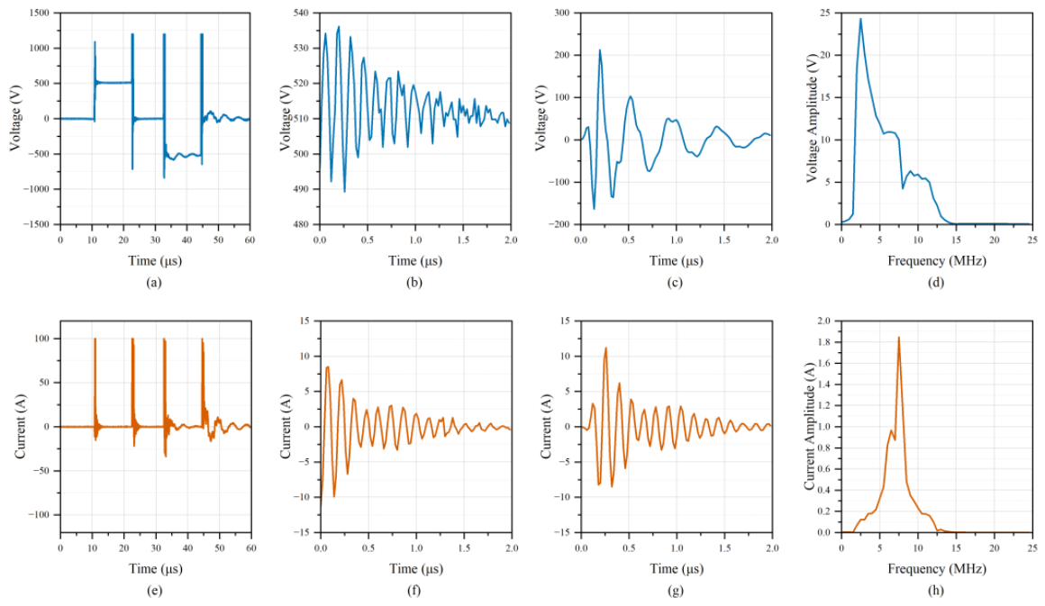
Figure 9.
Processing of the synchronized voltage and insulation-current waveforms: (a) original voltage waveform; (b) windowed 2 μs voltage segment extracted at the positive-polarity rising edge; (c) band-pass-filtered voltage response; (d) voltage amplitude spectrum; (e) original insulation-current waveform; (f) windowed 2 μs current segment; (g) band-pass-filtered current response; and (h) current amplitude spectrum.
Figure 9.
Processing of the synchronized voltage and insulation-current waveforms: (a) original voltage waveform; (b) windowed 2 μs voltage segment extracted at the positive-polarity rising edge; (c) band-pass-filtered voltage response; (d) voltage amplitude spectrum; (e) original insulation-current waveform; (f) windowed 2 μs current segment; (g) band-pass-filtered current response; and (h) current amplitude spectrum.
3.2. FFT-Based Dominant-Frequency Impedance Feature
A 100-point fast Fourier transform was applied separately to the filtered voltage and current segments without zero padding using the FFT Spectrum (Mag-Phase) VI in LabVIEW. Let and denote the voltage- and current-spectrum magnitudes at frequency bin k and aging time t, respectively. Because the voltage and current signals were synchronously sampled and processed using the same segment and FFT length, the spectral components at the same frequency bin were used to calculate the impedance magnitude. The Butterworth Filter VI was reinitialized for each waveform record, and the voltage and current channels were processed independently to prevent filter-state transfer between records or channels.
The FFT frequency resolution was
where is the sampling frequency and is the FFT length. After band-pass filtering, the frequency bin corresponding to the maximum current-spectrum magnitude within the 2–12 MHz analysis band was determined as
where denotes the set of FFT bins within the analysis band. The corresponding dominant frequency was calculated as
The impedance magnitude at the identified frequency was calculated from the voltage- and current-spectrum magnitudes at the same frequency bin:
The aging feature was subsequently defined as the product of the impedance magnitude and the corresponding dominant frequency:
where is expressed in MHz. Therefore, has units of Ω·MHz. Only one dominant frequency was used for each diagnostic waveform, and no arithmetic averaging across multiple frequency points was performed. Because the proposed feature was constructed from spectral magnitudes, the phase angles of the voltage and current spectra were not included in its calculation.
The frequency-weighted impedance is related to the effective capacitance of the winding-to-ground insulation. For an ideal capacitive response,
and therefore
Thus, the proposed feature is approximately proportional to the inverse of the effective insulation capacitance. Actual winding insulation is not an ideal capacitor; thermal aging also changes dielectric loss, conductivity, interfacial conditions, and structural integrity. The proposed feature should therefore be interpreted as a degradation-sensitive frequency-domain indicator rather than an exact capacitance measurement.
The principal signal-processing parameters used for feature extraction are summarized in Table 2.
3.3. Temperature Dependence of the Frequency-Weighted Impedance Feature
The electrical parameters of winding insulation are affected by both irreversible aging and reversible temperature variation. Consequently, features measured at different specimen temperatures cannot be compared directly. To distinguish the long-term aging trend from the short-term temperature effect, the variation in with specimen temperature was measured during the cooling stage of each aging subcycle.
After a specimen was removed from the 300 °C aging environment, its temperature gradually decreased during the diagnostic stage. Bipolar-pulse measurements were performed at multiple temperatures during this cooling process. For aging state s, a series of feature–temperature data pairs was obtained:
where is the specimen temperature at the m-th measurement, is the corresponding insulation-impedance feature, and is the number of valid measurements obtained during the cooling process.
The measured feature–temperature relationship was fitted using the least-squares method. A first-order fitting model was expressed as
where as and bs are the fitted temperature coefficient and intercept for aging state s, respectively. The coefficients were determined by minimizing
The least-squares solution can be written as
where
Figure 10 shows a representative set of insulation-impedance features measured during specimen cooling and the corresponding least-squares fitting result. As shown in Figure 10a, the individual measurements exhibited noticeable short-term fluctuations, whereas the systematic variation in FZ over the investigated temperature range was relatively small. Therefore, the fitted relationship is presented separately in Figure 10b using an enlarged vertical scale. The fitted feature exhibited a weak decreasing trend with increasing temperature. Although this systematic variation was small relative to the point-to-point fluctuations, temperature normalization was applied consistently to avoid introducing a temperature-dependent bias into the aging trajectory.
3.4. Feature Correction to the Reference Temperature
A reference temperature of 85 °C was selected to compare features obtained during different aging subcycles. For aging state s, the temperature-corrected insulation-impedance feature was calculated from the fitted model as
Thus, the multiple feature values measured during one cooling process were converted into a single characteristic value referenced to 85 °C. The corrected feature , rather than a value measured at an arbitrary instantaneous temperature, was used in the subsequent degradation analysis.
The representative fit in Figure 10 yielded only a small slope and a low coefficient of determination; therefore, no strong linear temperature dependence is inferred from this example. The transformation to 85 °C was nevertheless retained as a common reference convention and was applied identically at every aging state. Accordingly, temperature referencing was used to standardize the diagnostic condition rather than to imply that temperature variation was the dominant source of feature variability.
For specimen i, the corrected feature trajectory was expressed as
where ti,j is the cumulative aging time at the j-th diagnostic measurement, is the corresponding temperature-corrected feature, and Ji is the number of valid diagnostic measurements obtained from specimen i.
Because the duration of an individual aging subcycle varied from 0.6 to 24.2 h, the corrected feature values were arranged according to the actual cumulative aging time rather than the subcycle number. This treatment preserved the true temporal spacing between successive measurements.
As shown in Figure 11, the temperature-corrected feature exhibited substantial short-term fluctuations and was not strictly monotonic. Because is approximately inversely proportional to the effective insulation capacitance, the capacitance-based criterion corresponds to . The initial feature value was 13.7076 Ω·MHz; therefore, the fixed feature threshold was 27.4152 Ω·MHz. The first measured value exceeding this threshold was 38.7165 Ω·MHz at 428.405 h. This threshold crossing coincided with the independently confirmed capacitance-based EOL at the same diagnostic point. All measurements obtained after this point were excluded from the lifetime-prediction dataset.
3.5. Lifetime-Prediction Dataset Construction
After waveform processing and temperature correction, each valid diagnostic record was represented by its actual cumulative aging time and one temperature-corrected dominant-frequency impedance feature. For the specimen used in the lifetime analysis, the chronological dataset was
The data covered the interval from 0 to 428.405 h and included the first measurement that exceeded the fixed end-of-life threshold. Measurements acquired after that first crossing were excluded. Because the aging-subcycle duration varied from 0.6 to 24.2 h, actual cumulative aging time, rather than the subcycle index, was used as the temporal coordinate.
At rolling prediction origin , only measurements acquired no later than that time were available for model development:
The GPR model forecast the future feature trajectory rather than directly regressing RUL. The predicted end-of-life time was obtained from the first crossing of the forecast feature trajectory and the fixed threshold, after which RUL was calculated as the difference between the predicted end-of-life time and the current prediction origin. This chronological construction prevented future measurements from entering an earlier prediction stage but did not constitute independent specimen-level validation.
4. GPR-Based Insulation Lifetime Prediction Method
4.1. Rolling Feature-Trajectory Forecasting
At prediction origin , the training set consisted of all temperature-corrected feature measurements available up to and including . Each newly acquired measurement initiated a complete model update. Thus, the predicted end-of-life time was allowed to move either earlier or later as additional degradation information became available; no inter-update end-of-life locking rule was applied.
The regression input was cumulative aging time, and the regression response was the temperature-corrected feature. The observation model was expressed as
where is the latent degradation trajectory and represents measurement noise and short-term variability. RUL was not used as the regression target.
4.2. Causal Preprocessing and Monotonic Trend Extraction
The measured feature contained substantial point-to-point fluctuations. To reduce their influence without using future observations, a seven-point causal arithmetic mean was calculated at each prediction stage:
where
The filtered value therefore depended only on the current and previous measurements. Because the measurement intervals were irregular, this operation was a seven-record moving average rather than a fixed-duration time filter.
A nondecreasing latent degradation sequence was subsequently extracted using isotonic regression:
This step represented the irreversible long-term component of insulation degradation while preventing temporary downward fluctuations from dominating long-range extrapolation.
4.3. Quadratic Mean Function and Residual GPR
At each prediction stage, a quadratic mean function was fitted to the isotonic degradation sequence:
The quadratic coefficients were first estimated by least squares. The extrapolative slope and curvature were then restricted to nonnegative values, and the intercept was not allowed to fall below the final isotonic trend value. These restrictions prevented the long-term mean function from producing a physically inconsistent decreasing degradation trajectory.
The residuals between the causally averaged measurements and the quadratic mean were calculated as
and modeled using a zero-mean Gaussian process:
A Matérn-3/2 covariance kernel was adopted:
where is the residual signal standard deviation and is the characteristic time scale. Independent Gaussian observation noise with standard deviation was added to the diagonal of the covariance matrix:
The hyperparameters were selected by minimizing the negative log marginal likelihood:
The residual process was restricted to short-memory behavior by limiting to 5 h, which is comparable to the average aging-subcycle duration of 4.3 h. Candidate length scales consisted of eight logarithmically spaced values from 0.75 to 5 h. Let denote the standard deviation of the available residuals. The candidate signal standard deviations were
and the candidate noise standard deviations were
The hyperparameter combination with the minimum negative log marginal likelihood was selected independently at each rolling update.
For a future time , the predicted feature mean was
4.4. Monotonic Forecast and Threshold-Crossing RUL
The posterior-mean feature forecast was evaluated on a 0.25 h grid extending from the current prediction origin to a maximum aging time of 800 h. To represent irreversible long-term degradation, the future mean forecast was converted into a nondecreasing sequence:
This within-forecast monotonic constraint is distinct from locking successive end-of-life estimates. When a new measurement became available, the complete model was refitted, and the predicted end-of-life time could move either earlier or later.
The predicted end-of-life time was defined as the first future crossing of the fixed threshold:
Linear interpolation between adjacent grid points was used to refine the threshold-crossing time. The predicted RUL was calculated as
Figure 12.
Workflow of the rolling feature-trajectory GPR method for winding-insulation RUL prediction.
Figure 12.
Workflow of the rolling feature-trajectory GPR method for winding-insulation RUL prediction.
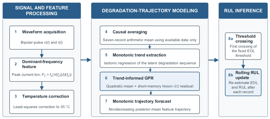
The proposed procedure consists of bipolar-pulse waveform acquisition, dominant-frequency feature extraction, temperature correction, chronological training-data selection, seven-point causal averaging, isotonic degradation-trend extraction, quadratic-mean fitting, short-memory Matérn-3/2 residual GPR, monotonic future feature-trajectory forecasting, and threshold-crossing-based calculation of end-of-life time and RUL.
4.5. Chronological Evaluation Metrics
The experimentally observed lifetime was h. The actual RUL at prediction origin was calculated retrospectively as
The absolute error was
The bounded relative accuracy was defined as
For valid rolling predictions, the mean absolute error was
the root-mean-square error was
and the mean bounded relative accuracy was
Rolling prediction was evaluated at every nonterminal diagnostic measurement after 80% of the observed lifetime. Since
ten prediction origins from 345.553 to 424.220 h were included. The end-of-life measurement at 428.405 h was used only to establish the observed failure time and was not used as a prediction origin.
5. Results and Discussion
5.1. Evolution of the Frequency-Weighted Impedance Feature
Figure 11 presents the complete temperature-corrected feature trajectory. The measured feature was strongly non-monotonic. It decreased from the initial value of 13.7076 Ω·MHz to approximately 5–7 Ω·MHz during the early part of the experiment and subsequently remained within a relatively low range for an extended period. A temporary excursion occurred between approximately 146 and 163 h, with a local maximum of 14.5340 Ω·MHz at 146.478 h, after which the feature returned to 5.8446 Ω·MHz at 165.230 h. This behavior demonstrates that an isolated feature increase cannot be interpreted directly as irreversible degradation.
A more persistent increase became visible after approximately 237 h, although substantial local reversals remained. The feature reached 21.1697 Ω·MHz at 329.900 h and exceeded 22 Ω·MHz at several later measurements. It subsequently decreased again before rising sharply to 38.7165 Ω·MHz at 428.405 h. This value was the first measurement exceeding the fixed threshold of 27.4152 Ω·MHz and coincided with the independently confirmed capacitance-based EOL at 428.405 h.
The non-monotonic measurements motivated separation of the long-term degradation trend from short-term fluctuations. The lifetime model therefore did not convert an individual feature measurement directly into RUL. Instead, it forecast the chronological feature trajectory and calculated RUL from the predicted future threshold-crossing time.
5.2. Rolling RUL Prediction Results
The rolling evaluation began after 80% of the observed lifetime. At each of the ten nonterminal diagnostic times, the current measurement was appended to the available sequence, the complete preprocessing and GPR procedure was repeated, and a new end-of-life time and RUL were calculated. All ten prediction stages produced a finite threshold crossing.
The predicted end-of-life time remained close to the observed value during most of the late-life sequence. For prediction origins from 345.553 to 389.132 h, the bounded RA ranged from 91.56% to 98.48%. The highest bounded RA, 98.48%, was obtained at 373.515 h, when the predicted RUL was 54.055 h and the actual RUL was 54.890 h.
The bounded RA decreased at the final three prediction origins. At 394.548 and 400.055 h, the feature remained below the threshold and contained local decreases, causing the model to postpone the predicted threshold crossing. At 424.220 h, only 4.185 h of actual life remained, whereas the forecast threshold crossing occurred at 450.963 h. The resulting bounded RA was zero according to the definition in Equation (40). This result shows that an abrupt terminal increase cannot be anticipated accurately from preceding measurements that do not yet contain the same change.
5.3. Aggregate Performance and RUL Evolution
Across the ten rolling prediction origins, the mean bounded relative accuracy was 80.08%, the MAE was 6.455 h, the RMSE was 8.923 h, and the finite-prediction rate was 100%. Because negative relative-accuracy values were truncated to zero, the bounded mean RA should be interpreted together with the pointwise results in Table 3 and the absolute-error metrics rather than as an unbiased estimate of generalization accuracy.
Figure 13 presents representative feature-trajectory forecasts at selected rolling prediction origins. Each model was constructed using only measurements available up to the corresponding origin. Figure 14 compares the rolling predicted RUL with the actual RUL at all ten prediction origins.
The RUL estimate was recalculated after every new diagnostic measurement rather than generated only once at the beginning of the late-life stage. The predicted RUL generally followed the decreasing actual-RUL trajectory. However, its deviation increased immediately before failure because the terminal feature increase occurred abruptly between two diagnostic measurements.
5.4. Engineering Interpretation and Limitations
The proposed model combines a slowly varying degradation trend with a short-memory stochastic residual. The seven-point causal average and isotonic regression reduce the influence of temporary excursions, while the quadratic mean function represents the long-term increase toward failure. The Matérn-3/2 residual process describes local deviations without allowing them to dominate long-range extrapolation. Because the model is refitted after every measurement, the RUL estimate adapts to newly observed degradation information.
Only posterior-mean threshold crossings were evaluated in this proof-of-concept study. Predictive uncertainty in the feature trajectory was not propagated to probabilistic EOL or RUL intervals. Future work should propagate the GPR posterior uncertainty through the threshold-crossing procedure to obtain probabilistic EOL and RUL intervals.
The results also reveal an important limitation. The final threshold crossing was associated with an abrupt increase from 17.1879 Ω·MHz at 424.220 h to 38.7165 Ω·MHz at 428.405 h. A model trained only on measurements up to 424.220 h could not know in advance that this abrupt increase would occur during the next interval. Consequently, the final rolling prediction produced a large relative error. More frequent diagnostic measurements near failure or additional degradation-sensitive features may improve terminal-stage prediction.
Because the aging temperature of 300 °C substantially exceeded the 180 °C thermal class of the investigated insulation system, the present results do not establish an Arrhenius acceleration factor or a direct conversion to field service life. Tests at multiple aging temperatures are required to verify degradation-mechanism consistency and support service-life extrapolation.
Only one complete physical lifetime trajectory was used. The model structure, seven-point causal-averaging width, and hyperparameter-search limits were developed using this same trajectory. At each rolling prediction origin, future measurements were excluded from model fitting; however, the rolling origins remained statistically dependent because they were obtained from the same specimen, and the overall modeling choices were not evaluated using an independent lifetime trajectory. Therefore, the reported 80.08% mean bounded relative accuracy should be regarded as a retrospective proof-of-concept result rather than an unbiased estimate of specimen-level generalization performance. Future studies should use multiple complete specimens, specimen-level external validation, different aging temperatures, and combined thermal, electrical, mechanical, and environmental stresses.
6. Conclusions
This study developed a waveform-feature-based RUL prediction method for the main insulation of electric-vehicle traction-motor windings. Simulated winding modules were subjected to full-lifecycle accelerated thermal aging at 300 °C, and synchronized voltage and insulation-current waveforms were acquired at 50 MSPS under bipolar high-voltage pulse excitation.
A 2 μs oscillatory segment associated with the positive-polarity rising edge was processed using a Hann window, a 10th-order Butterworth band-pass filter from 2 to 12 MHz, and a 100-point FFT. The frequency bin with the maximum current-spectrum magnitude was identified. The voltage-to-current spectral-magnitude ratio at the same frequency was used to calculate the impedance magnitude, which was multiplied by the corresponding frequency to obtain in Ω·MHz. Thus, each diagnostic waveform yielded a single dominant-frequency feature rather than an arithmetic average of characteristics obtained at multiple frequency points.
The complete modeling trajectory contained 119 diagnostic measurements. The initial feature was 13.7076 Ω·MHz, and the fixed end-of-life threshold was 27.4152 Ω·MHz. The first measured threshold crossing occurred at 428.405 h, where the feature reached 38.7165 Ω·MHz. Measurements acquired after this point were excluded.
A trend-informed GPR model was developed using a seven-point causal average, isotonic degradation-trend extraction, a nondecreasing quadratic mean function, and a short-memory Matérn-3/2 residual process. After each new measurement, the model was completely updated, and a new RUL was obtained from the first crossing of the predicted feature trajectory and the fixed threshold. No inter-update end-of-life locking rule was used.
Ten rolling prediction origins after 80% of the observed lifetime were evaluated. All predictions produced a finite RUL estimate. The mean bounded relative accuracy was 80.08%, with an MAE of 6.455 h and an RMSE of 8.923 h. The bounded RA exceeded 91% at the first seven rolling origins but decreased close to failure because the terminal feature increase occurred abruptly between two diagnostic measurements.
The results demonstrate the feasibility of the proposed chronological feature-trajectory method for the investigated specimen. However, the evaluation was based on one complete lifetime trajectory and does not establish specimen-independent generalization. Future work should include multiple full-lifecycle specimens, external specimen-level validation, shorter diagnostic intervals near failure, additional aging temperatures, and complete traction-motor stators under combined service stresses.
Author Contributions
Conceptualization, Q.S. and T.F.; methodology, Q.S.; software, Q.S.; validation, T.F.; formal analysis, T.F.; investigation, Q.S.; resources, Q.S.; data curation, T.F.; writing—original draft preparation, Q.S.; writing—review and editing, T.F.; visualization, Q.S.; supervision, T.F.; project administration, T.F.; funding acquisition, T.F. All authors have read and agreed to the published version of the manuscript.
Funding
This research was funded by National Basic Research Program, grant number DEDP2023007.
Data Availability Statement
The data supporting the findings of this study are available from the corresponding author upon reasonable request.
Acknowledgments
During the preparation of this manuscript, the authors used OpenAI Codex (GPT-5.6 Sol) to assist with language editing and structural organization. The authors have reviewed and edited the output and take full responsibility for the content of this publication.
Conflicts of Interest
The authors declare no conflicts of interest.
Abbreviations
The following abbreviations are used in this manuscript:
| ADC | Analog-to-digital converter |
| ARM | Advanced RISC Machines |
| DC | Direct current |
| EOL | End of life |
| FFT | Fast Fourier transform |
| FPGA | Field-programmable gate array |
| GPR | Gaussian process regression |
| IEC | International Electrotechnical Commission |
| MAE | Mean absolute error |
| MSPS | Mega-samples per second |
| RA | Relative accuracy |
| RMSE | Root-mean-square error |
| RUL | Remaining useful life |
| SoC | System on chip |
References
- Petri, T.; Keller, M.; Parspour, N. The Insulation Resilience of Inverter-Fed Low Voltage Traction Machines: Review, Challenges, and Opportunities. IEEE Access 2022, 10, 104023–104049. [CrossRef]
- Xu, Y.; Yuan, X.; Ye, F.; Wang, Z.; Zhang, Y.; Diab, M.; Zhou, W. Impact of High Switching Speed and High Switching Frequency of Wide-Bandgap Motor Drives on Electric Machines. IEEE Access 2021, 9, 82866–82880. [CrossRef]
- Melfi, M.J. Low-Voltage PWM Inverter-Fed Motor Insulation Issues. IEEE Trans. Ind. Appl. 2006, 42, 128–133. [CrossRef]
- Ghassemi, M. Accelerated Insulation Aging Due to Fast, Repetitive Voltages: A Review Identifying Challenges and Future Research Needs. IEEE Trans. Dielectr. Electr. Insul. 2019, 26, 1558–1568. [CrossRef]
- Kaufhold, M.; Aninger, H.; Berth, M.; Speck, J.; Eberhardt, M. Electrical Stress and Failure Mechanism of the Winding Insulation in PWM-Inverter-Fed Low-Voltage Induction Motors. IEEE Trans. Ind. Electron. 2000, 47, 396–402. [CrossRef]
- Kaufhold, M.; Börner, G.; Eberhardt, M.; Speck, J. Failure Mechanism of the Interturn Insulation of Low Voltage Electric Machines Fed by Pulse-Controlled Inverters. IEEE Electr. Insul. Mag. 1996, 12, 9–16. [CrossRef]
- Yin, W. Failure Mechanism of Winding Insulations in Inverter-Fed Motors. IEEE Electr. Insul. Mag. 1997, 13, 18–23. [CrossRef]
- Persson, E. Transient Effects in Application of PWM Inverters to Induction Motors. IEEE Trans. Ind. Appl. 1992, 28, 1095–1101. [CrossRef]
- Sundeep, S.; Wang, J.; Griffo, A.; Alvarez-Gonzalez, F. Anti-Resonance Phenomenon and Peak Voltage Stress within PWM Inverter Fed Stator Winding. IEEE Trans. Ind. Electron. 2021, 68, 11826–11836. [CrossRef]
- Hu, B.; Wei, Z.; You, H.; Na, R.; Liu, R.; Xiong, H.; Fu, P.; Zhang, J.; Wang, J. A Partial Discharge Study of Medium-Voltage Motor Winding Insulation under Two-Level Voltage Pulses with High dv/dt. IEEE Open J. Power Electron. 2021, 2, 225–235. [CrossRef]
- Lee, H.; Kim, H.; Jeong, J.; Lee, K.; Lee, S.B.; Stone, G. Inverter-Embedded Partial Discharge Testing for Reliability Enhancement of Stator Winding Insulation in Low Voltage Machines. IEEE Trans. Ind. Appl. 2022, 58, 2088–2096. [CrossRef]
- Wang, P.; Xu, H.; Wang, J.; Wang, W.; Cavallini, A. Effect of Repetitive Impulsive Voltage Duty Cycle on Partial Discharge Features and Insulation Endurance of Enameled Wires for Inverter-Fed Low Voltage Machines. IEEE Trans. Dielectr. Electr. Insul. 2017, 24, 2123–2131. [CrossRef]
- Fabiani, D.; Montanari, G.C.; Cavallini, A.; Mazzanti, G. Relation between Space Charge Accumulation and Partial Discharge Activity in Enameled Wires under PWM-Like Voltage Waveforms. IEEE Trans. Dielectr. Electr. Insul. 2004, 11, 393–405. [CrossRef]
- Sun, P.; Sima, W.; Jiang, X.; Zhang, D.; He, J.; Ye, L. Review of Accumulative Failure of Winding Insulation Subjected to Repetitive Impulse Voltages. High Volt. 2019, 4, 1–11. [CrossRef]
- Zoeller, C.; Vogelsberger, M.A.; Fasching, R.; Grubelnik, W.; Wolbank, T.M. Evaluation and Current-Response-Based Identification of Insulation Degradation for High Utilized Electrical Machines in Railway Application. IEEE Trans. Ind. Appl. 2017, 53, 2679–2689. [CrossRef]
- Sciascera, C.; Gerada, C.; Galea, M.; Giangrande, P. Lifetime Consumption and Degradation Analysis of the Winding Insulation of Electrical Machines. In Proceedings of the 8th IET International Conference on Power Electronics, Machines and Drives (PEMD 2016), Glasgow, UK, 19–21 April 2016. [CrossRef]
- Zhou, X.; Giangrande, P.; Ji, Y.; Zhao, W.; Ijaz, S.; Galea, M. Insulation for Rotating Low-Voltage Electrical Machines: Degradation, Lifetime Modeling, and Accelerated Aging Tests. Energies 2024, 17, 1987. [CrossRef]
- Grubic, S.; Aller, J.M.; Lu, B.; Habetler, T.G. A Survey on Testing and Monitoring Methods for Stator Insulation Systems of Low-Voltage Induction Machines Focusing on Turn Insulation Problems. IEEE Trans. Ind. Electron. 2008, 55, 4127–4138. [CrossRef]
- International Electrotechnical Commission. IEC 60034-18-41:2014+AMD1:2019, Rotating Electrical Machines—Part 18-41: Partial Discharge Free Electrical Insulation Systems (Type I) Used in Rotating Electrical Machines Fed from Voltage Converters—Qualification and Quality Control Tests; IEC: Geneva, Switzerland, 2019.
- International Electrotechnical Commission. IEC 60034-18-42:2017+AMD1:2020, Rotating Electrical Machines—Part 18-42: Partial Discharge Resistant Electrical Insulation Systems (Type II) Used in Rotating Electrical Machines Fed from Voltage Converters—Qualification Tests; IEC: Geneva, Switzerland, 2020.
- International Electrotechnical Commission. IEC 60034-18-21:2012, Rotating Electrical Machines—Part 18-21: Functional Evaluation of Insulation Systems—Test Procedures for Wire-Wound Windings—Thermal Evaluation and Classification; IEC: Geneva, Switzerland, 2012.
- Akram, S.; Liu, X.; Wang, P.; Meng, P.; Castellon, J.; Cavallini, A. Design of a Rectangular Wave High Voltage Generator for the Evaluation of Inverter-Fed Motor Insulation. IEEE Trans. Ind. Electron. 2023, 70, 4485–4493. [CrossRef]
- Rasmussen, C.E.; Williams, C.K.I. Gaussian Processes for Machine Learning; MIT Press: Cambridge, MA, USA, 2006; ISBN 978-0-262-18253-9.
- Saha, B.; Goebel, K.; Poll, S.; Christophersen, J. Prognostics Methods for Battery Health Monitoring Using a Bayesian Framework. IEEE Trans. Instrum. Meas. 2009, 58, 291–296. [CrossRef]
- Liu, J.; Chen, Z. Remaining Useful Life Prediction of Lithium-Ion Batteries Based on Health Indicator and Gaussian Process Regression Model. IEEE Access 2019, 7, 39474–39484. [CrossRef]
- Kang, W.; Xiao, J.; Xiao, M.; Hu, Y.; Zhu, H.; Li, J. Research on Remaining Useful Life Prognostics Based on Fuzzy Evaluation–Gaussian Process Regression Method. IEEE Access 2020, 8, 71965–71973. [CrossRef]
Figure 1.
Configuration of the winding insulation test specimen: (a) schematic diagram; (b) physical prototype.
Figure 1.
Configuration of the winding insulation test specimen: (a) schematic diagram; (b) physical prototype.
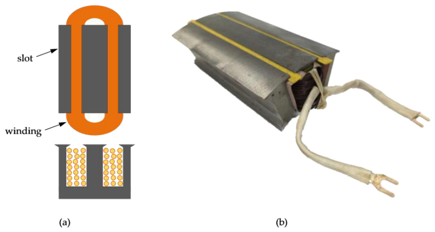
Figure 3.
Flowchart of the full-lifecycle accelerated thermal-aging experiment and periodic bipolar-pulse measurement procedure.
Figure 3.
Flowchart of the full-lifecycle accelerated thermal-aging experiment and periodic bipolar-pulse measurement procedure.
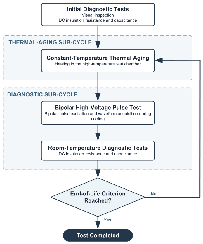
Figure 4.
Winding-insulation specimens at different stages of the constant-temperature accelerated lifetime test: (a) before aging; (b) during aging; and (c) after failure.
Figure 4.
Winding-insulation specimens at different stages of the constant-temperature accelerated lifetime test: (a) before aging; (b) during aging; and (c) after failure.
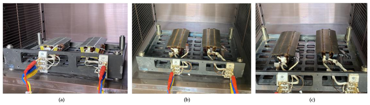
Figure 5.
Functional architecture of the dedicated bipolar high-voltage pulse test system.
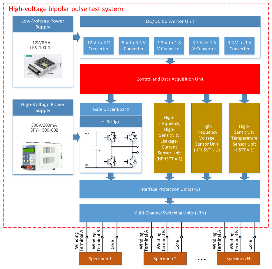
Figure 6.
Electrical connection of the winding-module specimen, bipolar-pulse source, and voltage and leakage-current sensors.
Figure 6.
Electrical connection of the winding-module specimen, bipolar-pulse source, and voltage and leakage-current sensors.
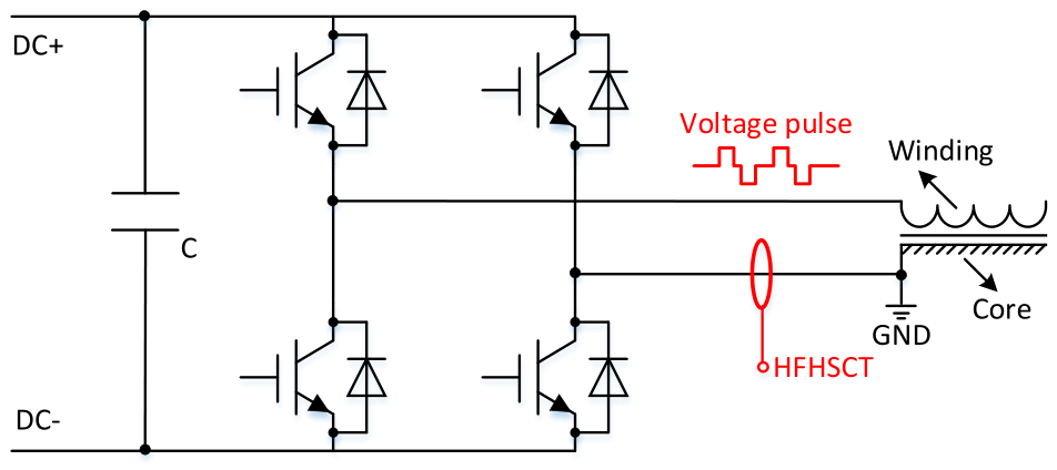
Figure 7.
Developed bipolar high-voltage pulse test platform: (a) three-dimensional structural model; (b) arrangement of the functional modules; and (c) physical prototype.
Figure 7.
Developed bipolar high-voltage pulse test platform: (a) three-dimensional structural model; (b) arrangement of the functional modules; and (c) physical prototype.
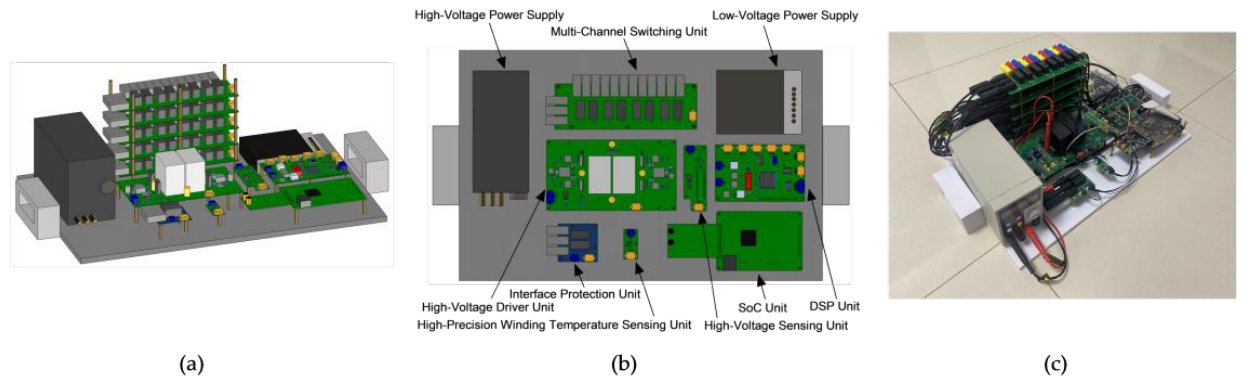
Figure 8.
Representative synchronized bipolar-pulse voltage v(t) and insulation-current i(t) waveforms acquired from a winding-module specimen.
Figure 8.
Representative synchronized bipolar-pulse voltage v(t) and insulation-current i(t) waveforms acquired from a winding-module specimen.
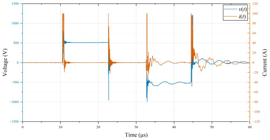
Figure 10.
Temperature dependence and least-squares fitting of the frequency-weighted impedance feature during specimen cooling: (a) measured feature values at different temperatures; and (b) fitted temperature–feature relationship shown using an enlarged vertical scale.
Figure 10.
Temperature dependence and least-squares fitting of the frequency-weighted impedance feature during specimen cooling: (a) measured feature values at different temperatures; and (b) fitted temperature–feature relationship shown using an enlarged vertical scale.
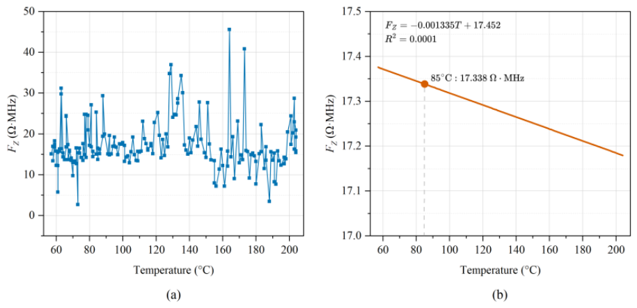
Figure 11.
Evolution of the dominant-frequency impedance feature corrected to 85 °C with cumulative aging time.
Figure 11.
Evolution of the dominant-frequency impedance feature corrected to 85 °C with cumulative aging time.
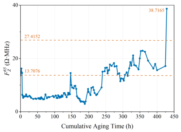
Figure 13.
Representative rolling forecasts at prediction origins of (a) 345.553 h, (b) 373.515 h, and (c) 400.055 h. Filled and open markers denote measurements available to and withheld from the model, respectively; the horizontal dashed line denotes the fixed EOL threshold.
Figure 13.
Representative rolling forecasts at prediction origins of (a) 345.553 h, (b) 373.515 h, and (c) 400.055 h. Filled and open markers denote measurements available to and withheld from the model, respectively; the horizontal dashed line denotes the fixed EOL threshold.
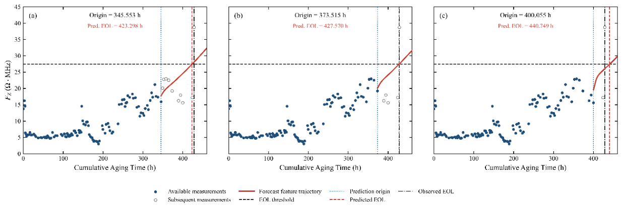
Figure 14.
Comparison between the rolling predicted RUL and the actual RUL after 80% of the observed insulation lifetime.
Figure 14.
Comparison between the rolling predicted RUL and the actual RUL after 80% of the observed insulation lifetime.
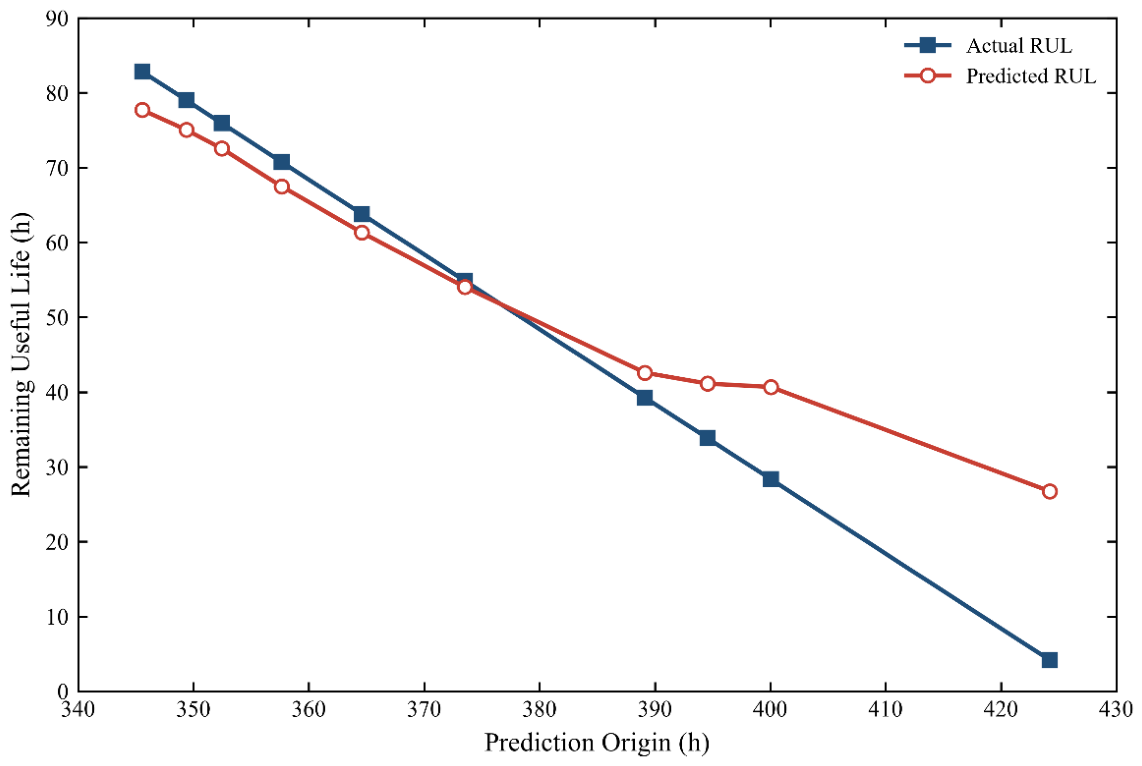

Table 1.
Accelerated-aging, bipolar-pulse measurement, and lifetime-definition parameters.
| Parameter | Symbol | Value |
| Number of simulated winding modules | N | 2 |
| Aging temperature | Tage | 300 °C |
| Aging-subcycle duration | Δtage | 4.3 h on average (0.6–24.2 h) |
| Bipolar pulse magnitude | Vp | ±0.5 kV |
| Pulse repetition frequency | fp | 0.1 Hz |
| Pulse rise/fall time | tr/tf | 20 ns |
| Pulse width | tp | 10 μs |
| Voltage sampling rate | fs,V | 50 MSPS |
| Current sampling rate | fs,I | 50 MSPS |
| End-of-life criterion | EOL | Winding-to-ground capacitance below 50% of its initial value or insulation resistance below 10 MΩ |
Table 2.
Signal-processing parameters used for dominant-frequency impedance-feature extraction.
| Processing Parameter | Symbol | Value |
| Original waveform duration | 60 μs | |
| Sampling rate | 50 MSPS | |
| Sampling interval | 20 ns | |
| Selected switching transition | Positive-polarity rising edge | |
| Extracted segment duration | 2 μs | |
| Number of samples per segment | 100 | |
| Window function | Hann window | |
| Filter type | 10th-order Butterworth band-pass filter | |
| Band-pass frequency range | 2–12 MHz | |
| FFT length | 100 points | |
| Zero padding | None | |
| Frequency resolution | 0.5 MHz | |
| Dominant-frequency search range | 2–12 MHz | |
| Peak-selection criterion | Maximum current-spectrum magnitude | |
| Spectral points used per feature | — | One dominant-frequency bin |
| Reference temperature | 85 °C |
Table 3.
Rolling end-of-life and RUL prediction results after 80% of the observed lifetime.
| Prediction origin (h) | Predicted EOL (h) | Predicted RUL (h) | Actual RUL (h) | Absolute error (h) | Bounded RA (%) |
| 345.553 | 423.298 | 77.745 | 82.852 | 5.107 | 93.84 |
| 349.380 | 424.432 | 75.052 | 79.025 | 3.973 | 94.97 |
| 352.450 | 425.012 | 72.562 | 75.955 | 3.393 | 95.53 |
| 357.643 | 425.139 | 67.496 | 70.762 | 3.266 | 95.38 |
| 364.595 | 425.933 | 61.338 | 63.810 | 2.472 | 96.13 |
| 373.515 | 427.570 | 54.055 | 54.890 | 0.835 | 98.48 |
| 389.132 | 431.720 | 42.588 | 39.273 | 3.315 | 91.56 |
| 394.548 | 435.689 | 41.141 | 33.857 | 7.284 | 78.49 |
| 400.055 | 440.749 | 40.694 | 28.350 | 12.344 | 56.46 |
| 424.220 | 450.963 | 26.743 | 4.185 | 22.558 | 0.00 |
Disclaimer/Publisher’s Note: The statements, opinions and data contained in all publications are solely those of the individual author(s) and contributor(s) and not of MDPI and/or the editor(s). MDPI and/or the editor(s) disclaim responsibility for any injury to people or property resulting from any ideas, methods, instructions or products referred to in the content. |
© 2026 by the authors. Licensee MDPI, Basel, Switzerland. This article is an open access article distributed under the terms and conditions of the Creative Commons Attribution (CC BY) license (http://creativecommons.org/licenses/by/4.0/).
Copyright: This open access article is published under a Creative Commons CC BY 4.0 license, which permit the free download, distribution, and reuse, provided that the author and preprint are cited in any reuse.