

Submitted:
12 September 2026
Posted:
15 September 2026
You are already at the latest version
Abstract
Fractional heat-transport models provide a powerful framework for describing anomalous thermal diffusion and wave-like propagation. However, the same reduced fractional temperature equation may result from different energy–flux realizations, de-pending on whether the fractional dynamics is introduced through the energy balance, the heat-flux constitutive relation, or both. We investigate the consequences of this non-uniqueness for externally driven photothermal transport. We show that different realizations can have the same reduced propagation coefficient while exhibiting different characteristic thermal impedances and, consequently, different photothermal amplitude and phase responses. Thus, the reduced fractional propagation equation is not sufficient to characterize an externally driven thermal response. Photothermal measurements can provide additional information on the underlying energy–flux cou-pling and distinguish transport realizations that are indistinguishable at the level of the reduced fractional equation.
Keywords:
fractional heat transport
; subdiffusion
; fractional wave-like transport
; photothermal effect
; thermal impedance
1. Introduction
Photothermal experiments are based on the detection of the response of a material following the absorption of externally supplied optical energy [1,2,3,4]. The absorbed energy generates a temperature perturbation whose spatiotemporal evolution determines how the initial excitation propagates through the material and, ultimately, contributes to the formation of the photothermal signal. Therefore, describing the evolution of the optically generated temperature perturbation is an important element in modeling the photothermal signal, as well as in its analysis and physical interpretation [5].
Most traditional models of photothermal effects are based on the classical theory of heat conduction, namely Fourier’s law [6,7], which assumes an instantaneous local relation between the heat flux and the temperature gradient. However, numerous experimental and theoretical studies have shown that such a description may become inadequate when heat transport is considered on sufficiently small spatial and temporal scales, where memory effects, finite flux-relaxation times, and other forms of anomalous transport may become relevant [8,9,10,11,12].
In response to these limitations, various classical generalizations of Fourier’s theory have been developed [13,14,15,16,17]. These approaches, however, differ not only in the functional form introduced in place of Fourier’s law, but also in which part of the classical transport description is generalized. In some approaches, the energy conservation equation is modified, i.e., the way in which the energy dynamics is related to the temperature field is generalized [18,19]. In others, the constitutive relation between the heat flux and the temperature gradient is generalized, so that the heat flux acquires its own temporal dynamics or memory [20]. Formulations in which both parts of the transport description are generalized are also possible [21]. These different possibilities reflect different physical assumptions about the origin of memory and about the way in which energy and heat flux are coupled. This distinction becomes particularly important for fractional models, which provide a framework for describing a broad range of anomalous transport regimes and can be derived from different physical or mathematical constructions.
At the continuum level, a fractional operator may be introduced into the energy conservation equation, the constitutive relation [22], or both [21]. After elimination of the heat flux, however, different energy–flux realizations may lead to the same reduced equation for the temperature field [22,23,24,25,26]. Thus, different assumptions about the origin and distribution of memory may become indistinguishable at the level of the reduced homogeneous description.
This raises the question of what can be inferred from such a reduced description when transport is considered in a real problem involving an externally supplied energy excitation. The homogeneous reduced equation describes the propagation part of the problem for a specified preparation of the system and specified boundary conditions. By itself, however, it does not describe the external energy excitation. Moreover, for a finite system, it does not determine how the system interacts with its environment without additional assumptions concerning boundary or contact conditions. In a photothermal problem, in which energy is directly supplied to the system, it is therefore necessary to account also for the relation connecting the energy excitation, heat flux, and temperature field [27,28,29,30,31].
Two energy–flux realizations may have the same reduced propagation operator while exhibiting different relations between the heat flux and the temperature field. This difference becomes relevant when the experimental input is defined by an energy excitation, as in photothermal experiments, because the system response then depends not only on how the temperature perturbation propagates, but also on how the excitation is coupled to energy transport. In the frequency or Laplace domain, this additional information enters the thermal impedance, which determines the spectrum of the photothermal response. This highlights the particular role of photothermal experiments in probing the physical origin of non-Fourier and anomalous heat-conduction effects.
In this work, we investigate the relation between the reduced temperature description and the underlying energy–flux realization of heat transport. Starting from a general coupled system consisting of an energy conservation equation and heat-flux dynamics, we analyze how different realizations can lead to the same reduced homogeneous operator and where information about their underlying coupling is retained after reduction. As concrete examples, we consider subdiffusive transport [27,32,33,34,35] and generalized Cattaneo dynamics [22,28,29,30,31]. Their different realizations are then compared through the photothermal response of a finite system, with particular emphasis on thermal impedance as a quantity that can be sensitive to differences not contained in the reduced propagation operator itself.
The paper is organized as follows. Section 2 introduces the operator-based model and its reduction in the presence of a prescribed energy source. The reduction yields two operators: one governing the homogeneous temperature evolution and another describing the coupling to the excitation. We show that retaining only the homogeneous operator loses information about this coupling and permits infinitely many underlying realizations, depending on the preparation of the system. Section 3 considers two cases, subdiffusion and GCE-I, and shows how different realizations with the same homogeneous temperature dynamics can produce distinct thermal impedances. Section 4 summarizes the main conclusions and discusses the implications for identifying transport mechanisms from measured thermal responses.
2. Theoretical Background
2.1. Operator Form of the Reduced Transport Equation
We begin with the local energy conservation law,
where E denotes the energy density, J the heat flux, and S an external energy source. The energy density is related to the temperature field through a general temporal memory relation,
where KE denotes the corresponding temporal memory operator and (∗) denotes convolution in time.
∂tE(x,t)+∇∙J(x,t) = S(x,t),
E(x,t) = KE*T(x,t),
In addition to the memory contained in the energy sector, we assume an independent temporal dynamics of the heat flux, described by
ΛJJ(x,t) = −KJ*∇T(x,t).
The two operators appearing in Equation (3) have distinct roles. ΛJ describes the temporal dynamics of the heat flux, whereas KJ specifies its coupling to the thermodynamic driving force. Equation (3) can therefore be written in the operator form
with
provided that the convolution operator KJ is invertible.
ΛqJ(x,t) = −∇T(x,t)
Applying the operator Λq to Equation (1) and using Equation (2), we obtain
Since the operator Λq, act in time, they commute with spatial differentiation. Consequently, using Equation (4), we obtain
Λq∇∙J(x,t)=∇(ΛqJ(x,t)) = −∇2T(x,t)
The coupled system consisting of the energy balance, Equation (1), and the independent flux dynamics, Equation (3), can therefore be reduced to a single equation for the temperature field,
where
ΛTT(x,t) = ΛqS(x,t)
Equation (8) is the inhomogeneous reduced transport equation. It is important to retain the source term at this stage, because the same flux-dynamical operator that enters the elimination of the heat flux also acts on the external source.
If the volumetric source is neglected and the excitation is instead prescribed through the initial and boundary conditions,
ΛTT(x,t) = 0
Equation (10) is the form commonly used to characterize the evolution of the reduced temperature field. However, it contains only the effective operator ΛT, which results from the elimination of the heat flux.
This reduction has an important consequence. The original transport problem is defined by the coupled Equations (1) and (3), whereas Equation (10) contains only their reduced representation. In operator terms, the elimination of Λq is analogous to taking a Schur complement of a coupled block operator [36]. The resulting operator ΛT is an effective operator for the retained variable TT, but its decomposition into the underlying energy-memory and flux-dynamical operators is not, in general, unique. Thus, different coupled energy–flux systems may lead to the same reduced homogeneous operator,
while involving different flux-dynamical operators Λq. The homogeneous reduced equation therefore does not, by itself, uniquely identify the underlying energy–flux realization.
This distinction becomes essential once the system is externally driven. In the inhomogeneous Equation (8), the external source is acted upon by Λq. Consequently, information about the energy–flux coupling that is not contained in the homogeneous reduced operator re-enters through the source-to-response relation. The role of this information is examined below using the Green-function representation of the boundary-driven transport problem and its experimentally accessible thermal impedance.
2.2. Homogeneous Reduction and Operator Non-Uniqueness
The Green function of the reduced operator is defined by
ΛTGT(x,t;x.,t.) = δ(x − x.)δ(t − t.)
For a temperature-driven boundary problem (T(0,t) = T0(t)), ΛT characterizes the propagation generated by the reduced operator. However, the reduced operator and its Green function do not, by themselves, determine how a specific external energy excitation is coupled to the temperature field.
For the corresponding nonhomogeneous problem,
T(x,t) = GT*ΛqS(x,t)
Now consider two different underlying energy–flux realizations. They may produce the same reduced operator,
and, for the same domain and boundary conditions, the same Green function,
while having different source-coupling operators,
Consequently, the temperature responses to the same external energy excitation S need not be identical:
We refer to this non-uniqueness of the underlying energy–flux realization as operator degeneracy.
2.3. Photothermal Response
We now consider the photothermal problem in the Laplace domain. For a one-dimensional sample of thickness (L), the temperature field satisfies
The boundary conditions are imposed in terms of the heat flux,
where S0 denotes the amplitude of the impulsive thermal excitation applied at the illuminated surface (x=0). The heat flux is related to the temperature gradient by
The measured quantity is the temperature variation at the illuminated surface, (x=0). Solving the resulting boundary-value problem gives
or, equivalently,
We next express σ(s) and Zc(s) in terms of the Laplace-domain operators introduced in the general formulation. The reduced temperature equation can be written as
For the homogeneous problem, the temperature operator is represented as
Thus, the propagation coefficient σ(s) is determined by the temporal part of the reduced temperature operator.
For the heat flux, the reduced constitutive relation is
Hence.
Comparing this relation with the heat-flux relation used in Equation (20), we obtain
and therefore,
Consequently, the photothermal response can be expressed in terms of the two Laplace-domain operators, and . This is the key point for the following analysis. If two underlying transport realizations have the same reduced temperature operator, they have the same propagation coefficient,
σ(1)(s) = σ(2)(s)
However, they may involve different flux-dynamical operators, and therefore different characteristic impedances
Thus, although the two realizations obey the same homogeneous propagation equation, they can produce different photothermal responses (Equation (22)).
because the characteristic impedance retains information about the flux dynamics that is not contained in the reduced temperature operator alone.
T(1)(0,s) ≠ T(2)(0,s)
3. Case Studies: Subdiffusive Heat Transport and GCE I
3.1. Subdiffusive Heat Transport
We first consider the standard subdiffusive heat-transport equation formulated in terms of the Caputo fractional derivative. The reduced temperature equation is written as
where Dα is the generalized thermal diffusivity and denotes the Caputo derivative of order α,
For vanishing initial conditions, its Laplace-domain form is
and the corresponding propagation coefficient is
3.1.1. Realization I: Standard Energy Balance and Fractional Constitutive Relation
In the first realization, the standard energy balance is retained, while the fractional memory is introduced through the constitutive relation for the heat flux,
Taking the Laplace transform and assuming vanishing initial conditions gives
Comparing this relation with the general flux representation introduced above gives,
with
3.1.2. Realization II: Fractional Energy Balance and Classical Fourier Constitutive Relation
In the second realization, the fractional dynamics is introduced through the energy balance, while the constitutive relation remains classical and is given by Fourier’s law,
Taking the Laplace transform and assuming vanishing initial conditions gives,
Comparing this relation with the general flux representation introduced above gives,
with
Thus, for the subdiffusive equation, the two realizations can be summarized as follows:
| Model | Characteristic thermal impedance |
| SD memory in flux, | |
| SD memory in energy, |
The construction above follows directly from the operator reduction discussed in the preceding section: the reduced temperature equation determines the propagation coefficient σSD(s), whereas the particular realization of the energy–flux coupling determines the corresponding characteristic impedance.
The two realizations therefore share the same reduced propagation coefficient, while their characteristic impedances need not be identical. The consequences of this difference for the observable photothermal response are examined in subsection 3.3.
3.2. Generalized Cattaneo Equation I
We next consider the Generalized Cattaneo Equation I (GCE I) as a second case study [22]. As in the preceding case, we use the Caputo fractional derivative and consider the reduced temperature equation in the absence of volumetric sources. The purpose is to examine whether the same reduced GCE I operator can likewise be realized through different allocations of fractional dynamics within the underlying energy–flux description.
The GCE I equation contains, in addition to the fractional relaxation term, a second term involving the characteristic relaxation time τ. Starting from the reduced equation, we first determine the corresponding propagation coefficient σGCEI(s). We then construct two realizations of the same reduced equation, both of which involve a heat flux with its own temporal dynamics. The two realizations differ in how the fractional dynamics is incorporated into the underlying energy–flux description: in the first, it enters through the constitutive relation for the heat flux, while in the second, it is introduced through the energy balance in addition to the corresponding flux dynamics. For each realization, the characteristic impedance is obtained from the corresponding flux relation in the form introduced above.
Thus, as in the subdiffusive case, the two realizations share the same reduced propagation coefficient, while their characteristic impedances characterize the respective energy–flux couplings. The resulting impedances are subsequently used to determine the photothermal response and to examine the spectral consequences of the two realizations.
The reduced temperature equation for GCE I is written as [22]
where Dα is the generalized thermal diffusivity and denotes the Caputo derivative of order α (Equation (33)),
For vanishing initial conditions, its Laplace-domain form is
and the corresponding propagation coefficient is
3.2.1. Realization I: Standard Energy Balance and Fractional Flux Dynamics
In the first realization, the standard energy balance is retained, while the fractional dynamics is introduced through the constitutive relation for the heat flux [22],
Taking the Laplace transform and assuming vanishing initial conditions gives,
Comparing this relation with the general flux representation introduced above gives,
with
3.2.2. Realization II: Fractional Energy Balance and Fractional Flux Dynamics
In the second realization, the fractional dynamics is introduced through the energy balance, while the constitutive relation is given by the fractional Cattaneo law [22],
Taking the Laplace transform and assuming vanishing initial conditions gives.
Comparing this relation with the general flux representation introduced above gives.
with
Thus, for the GCEI equation, the two realizations can be summarized as follows:
| Model | Characteristic thermal impedance |
| GCEI fractional dynamics in constitutive relation, | |
| GCEI fractional dynamics in energy balance, |
The two realizations therefore share the same reduced propagation coefficient, while their characteristic impedances need not be identical. The consequences of this difference for the observable photothermal response are examined in the next section.
3.3. Spectral Consequences for the Photothermal Response
Having established the two realizations for each reduced transport operator, we now examine their consequences for the observable photothermal response. For the boundary-driven configuration considered here, the surface temperature is determined by Equations (21) and (22).
Since the two realizations of each reduced equation have the same propagation coefficient but different characteristic impedances, their photothermal responses can be directly compared in terms of amplitude and phase.
The analysis focused on a laser-sintered Polyamide (PA12) sample, ideal due to its characteristic porous structure. A very thin layer of black paint, whose properties can be neglected, is applied to provide surface absorption of incident radiation. The thermal characteristics of the PA12 are given in Table 1:
Figure 1 shows the amplitude (a) and phase (b) characteristics of temperature variations on the front side for subdiffusive transport for derivative orders α = 0.9 (red lines) and α = 0.5 (blue lines). For both derivative orders, two theories are presented. The first theory, which incorporates fractional memory through the constitutive relation for the heat flux, is represented by solid lines and is labeled SDq. The second theory, which introduces fractional dynamics through the energy balance while maintaining the classical constitutive relation defined by Fourier’s law, is illustrated by dashed lines and is labeled SDE.
The two realizations exhibit distinctly different amplitude and phase spectra despite having the same reduced subdiffusive propagation coefficient σSD(s) . Thus, the difference originates entirely from the different characteristic impedances associated with the two energy–flux closures. For lower orders of derivation, the differences increase.
In the limit α→1, the subdiffusive equation reduces to the classical diffusion equation. The fractional modification then disappears, and the two realizations reduce to the corresponding classical description. Consequently, this limiting case does not provide a distinction between the two fractional realizations.
Figure 2 illustrates the amplitude and phase characteristics of temperature variations on the front side of the sample for GCEI. Similar to Figure 1, the lines representing the theories being discussed are colored red for alpha = 0.9 and blue for alpha = 0.5. The solid lines depict the first realization with memory in flux, labeled as GCEIq, while the dashed lines represent the second realization with memory in energy balance, labeled as GCEIE.
As in the subdiffusive case, the two realizations of GCE I possess the same propagation coefficient σGCE, but produce substantially different amplitude and phase spectra because their characteristic impedances are different.
In the limit α→1, GCE I reduces to the classical hyperbolic heat-conduction equation. The two realizations then become identical, since the fractional modification of the energy balance disappears and both descriptions reduce to the same classical Cattaneo formulation. The corresponding amplitude and phase spectra therefore coincide.
The comparison of classical parabolic and hyperbolic limits further illustrates the role of flux dynamics, as shown in Figure 3. The blue lines represent the classical diffusion heat conduction model, while the red lines illustrate the hyperbolic heat conduction model.
For α=1, the subdiffusive model reduces to the classical diffusion equation, whereas GCE I reduces to the hyperbolic Cattaneo equation. Their different spectral responses therefore reflect the finite flux-relaxation time τ, representing a finite-memory effect rather than fractional memory.
When τ=0, the hyperbolic equation reduces to the parabolic diffusion equation, and the corresponding responses coincide. Thus, the difference between the parabolic and hyperbolic descriptions can itself be interpreted as a consequence of memory, with τ representing a finite memory time.
Thus, the difference between the parabolic and hyperbolic descriptions can itself be interpreted as a consequence of memory, with τ setting the characteristic time scale of the flux memory.
4. Conclusions
In this work, we have examined the relation between the reduced description of heat transport and the full energy–flux description in the context of fractional and other generalized transport models. Starting from a coupled system consisting of an energy conservation equation and heat-flux dynamics, we have shown that elimination of the heat flux leads to a reduced temperature equation whose homogeneous part defines the propagation operator for the specified problem. However, the homogeneous reduced equation itself does not contain the information required to describe an external energy excitation, nor does it determine the interaction of a finite system with its environment without additional assumptions concerning these couplings.
In particular, we have shown that different energy–flux realizations may possess the same homogeneous reduced operator, and therefore the same propagation coefficient, while differing in the way they relate the heat flux to the temperature field. This difference is not merely an alternative mathematical representation of the same experimental problem. When the system is externally excited by energy, the energy–flux relation becomes part of the input–output problem itself. In a photothermal experiment, this information enters through the characteristic thermal impedance and can lead to different temperature responses even when the reduced propagation operator is identical.
Subdiffusive transport and generalized Cattaneo dynamics provide two concrete examples of this behavior. In both cases, the considered realizations can be reduced to the same homogeneous propagation operator, while their characteristic impedances remain different. Consequently, the amplitude and phase of the photothermal response are not uniquely determined by the reduced anomalous equation alone. The classical limits further show how this difference disappears when fractional memory vanishes, whereas in the Cattaneo description the finite flux-relaxation time represents a distinct source of memory.
These results have an important implication for the interpretation of anomalous heat transport. Concepts such as anomalous diffusion or anomalous wave-like propagation characterize a particular form of spatiotemporal evolution, but do not, by themselves, determine a unique energy–flux realization of that behavior. The same propagation law may arise from different distributions of memory between the energy and flux sectors, and the distinction between such realizations can become physically relevant when the system is probed through an external energy excitation.
Thus, for describing propagation in a suitably prepared problem, the homogeneous reduced equation represents an essential level of description, but it is not sufficient for a complete description of an externally driven energy excitation. A photothermal experiment provides precisely this additional information: it probes not only how the temperature field propagates, but also how the supplied energy is coupled to the heat flux and the resulting temperature response. In this sense, the experimentally observed response can be used not only to characterize anomalous propagation, but also to distinguish between different physical realizations underlying the same reduced propagation equation.
Author Contributions
For research articles with several authors, a short paragraph specifying their individual contributions must be provided. The following statements should be used “Conceptualization, S,G; methodology, S,G.; software, M.P., M.J.P.,; validation, S.G., M.P. and M.J.P.; formal analysis, S.G., M.P. and M.J.P.; investigation, S.G., M.P. and M.J.P; writing—original draft preparation, S.G.,; writing—review and editing, S.G., M.P. and M.J.P.; visualization, S.G., M.P. and M.J.P; All authors have read and agreed to the published version of the manuscript.” Please turn to the CRediT taxonomy for the term explanation. Authorship must be limited to those who have contributed substantially to the work reported.
Funding
This research was funded by the Ministry of Science, Technological Development and Innovations of the Republic of Serbia (Contract No. 451-03-33/2026-03/ 200017).
Data Availability Statement
The data that supports the findings of this study are available from the corresponding author upon reasonable request.
References
- Vargas, H.; Miranda, L.C.M. Photoacoustic and related photothermal techniques. Phys. Rep. 1988, 161, 43–101. [Google Scholar] [CrossRef]
- Skvortsov, L.A. Laser photothermal spectroscopy of light-induced absorption. Quantum Electron. 2013, 43, 1–13. [Google Scholar] [CrossRef]
- Bialkowski, S.E.; Astrath, N.G.C.; Proskurnin, M.A. Photothermal Spectroscopy Methods, 2nd ed.; Wiley: Hoboken, NJ, USA, 2019; ISBN 978-1-119-27907-5. [Google Scholar] [CrossRef]
- Bertolotti, M.; Li Voti, R. A note on the history of photoacoustic, thermal lensing, and photothermal deflection techniques. J. Appl. Phys. 2020, 128, 230901. [Google Scholar] [CrossRef]
- 5. S. Galovic and S. Jacimovski, From Photothermal Transients to Effective Transport Operators: An Operator-Based Interpretation of TTG Dynamics. arXiv 2026, arXiv:2608.13813.
- Carslaw, H.S.; Jaeger, J.C. Conduction of Heat in Solids, 2nd ed.; Clarendon Press: Oxford, UK, 1959; ISBN 9780198533689. [Google Scholar]
- Mandelis, A. Diffusion-Wave Fields: Mathematical Methods and Green Functions; Springer: New York, NY, USA, 2001. [Google Scholar] [CrossRef]
- Peshkov, V. P. Second Sound in Helium II. J. Phys. 1944, 8, 381–389. [Google Scholar]
- Jackson, H. E.; Walker, C. T.; McNelly, T. F. Second Sound in NaF. Phys. Rev. Lett. 1970, 25, 26–28. [Google Scholar] [CrossRef]
- Huberman, S.; et al. Observation of second sound in graphite at temperatures above 100 K. Science 2019, 364, 375–379. [Google Scholar] [CrossRef] [PubMed]
- Xie, Z.; et al. Room-temperature second sound in isotopically pure graphite. Nat. Commun. 2026, 17, 4806. [Google Scholar] [CrossRef] [PubMed]
- Yao, F.; et al. Experimental Evidence of Superdiffusive Thermal Transport in Si₀.₄Ge₀.₆ Thin Films. Nano Lett. 2022, 22, 6888–6894. [Google Scholar] [CrossRef] [PubMed]
- Joseph, D. D.; Preziosi, L. Heat waves. Rev. Mod. Phys. 1989, 61, 41–95. [Google Scholar] [CrossRef]
- Novikov. Resonant generation of harmonic thermal waves in media with memory. J. Eng. Phys. Thermophys. 1992, 62, 367–372. [Google Scholar] [CrossRef]
- Tzou, D. Y. A unified field approach for heat conduction from macro- to micro-scales. J. Heat Transf. 1995, 117, 8–16. [Google Scholar] [CrossRef]
- Metzler, R.; Klafter, J. The random walk’s guide to anomalous diffusion: A fractional dynamics approach. Phys. Rep. 2000, 339, 1–77. [Google Scholar] [CrossRef]
- Mainardi, F. The fundamental solutions for the fractional diffusion-wave equation. Appl. Math. Lett. 1996, 9(6), 23–28. [Google Scholar] [CrossRef]
- Davies, R. O. The Macroscopic Theory of Irreversibility. Rep. Prog. Phys. 1956, 19, 326–377. [Google Scholar] [CrossRef]
- Tarasov, V. E. Nonlocal (general fractional) thermodynamics: Nonlocality on set of states. Ann. Phys. 2026, 493, 170606. [Google Scholar] [CrossRef]
- Jou, D.; Casas-Vázquez, J.; Lebon, G. Extended irreversible thermodynamics. Rep. Prog. Phys. 1988, 51, 1105–1179. [Google Scholar] [CrossRef]
- Galovic, 21 S.; Popovic, M. N.; Chevizovich, D. Electrical Analogy Approach to Fractional Heat Conduction Models. Fractal Fract. 2025, 9(10), 653. [Google Scholar] [CrossRef]
- Compte, 22; Metzler, R. The generalized Cattaneo equation for the description of anomalous transport processes. J. Phys. A Math. General. 1997, 30(21), 7277–7289. [Google Scholar] [CrossRef]
- Berkowitz, B.; Klafter, J.; Metzler, R.; Scher, H. Physical pictures of transport in heterogeneous media: Advection-dispersion, random-walk, and fractional derivative formulations. Water Resour. Res. 2002, 38, 9-1–9-12. [Google Scholar] [CrossRef]
- Barkai, E.; Metzler, R.; Klafter, J. From continuous time random walks to the fractional Fokker-Planck equation. Phys. Rev. E 2000, 61, 132–138. [Google Scholar] [CrossRef] [PubMed]
- Li, S.-N.; Cao, B.-Y. Fractional Boltzmann transport equation for anomalous heat transport and divergent thermal conductivity. Int. J. Heat Mass Transf. 2019, 137, 84–89. [Google Scholar] [CrossRef]
- Li, S.-N.; Cao, B.-Y. Fractional-order heat conduction models from generalized Boltzmann transport equation. Philos. Trans. R. Soc. A 2020, 378(2172), 20190280. [Google Scholar] [CrossRef] [PubMed]
- Galović et al., “Influence of Local Thermodynamic Non-Equilibrium to Photothermally Induced Acoustic Response of Complex Systems,” Fractal and Fractional. 2024, 8, 399. [CrossRef]
- Popovic, M. N.; Galovic, S. P.; Lenzi, E. K.; Somer, A. The Thermoelastic Component of the Photoacoustic Response in a 3D-Printed Polyamide Coated with Pigment Dye: A Two-Layer Model Incorporating Fractional Heat Conduction Theories. Fractal Fract. 2025, 9, 456. [Google Scholar] [CrossRef]
- Somer; Novatski, A.; da Cruz, G. K.; da Cruz, C. B. K.; Serbena, F. C.; Lenzi, E. K. Thermal fractional diffusion: experimental evidence from the discrepancies in the amplitude and phase in photothermal technique. Nonlinear Dyn. 2023, 111, 19265–19282. [Google Scholar] [CrossRef]
- Somer; Novatski, A.; Serbena, F. C.; Lenzi, E. K. Interplay between super and subdiffusive behaviors in photothermal phenomena. Int. J. Therm. Sci. 2021, 159, 106539. [Google Scholar] [CrossRef]
- Somer; Novatski, A.; Lenzi, M. K.; da Silva, L. R.; Lenzi, E. K. Fractional dual-phase-lag heat conduction with periodic heating and photo-thermal response. Therm. Sci. 2023, 27(3B), 2537–2547. [Google Scholar] [CrossRef]
- Wei, Q.; Wang, W.; Zhou, H.; Metzler, R.; Chechkin, A. Time-fractional Caputo derivative versus other integrodifferential operators in generalized Fokker–Planck and generalized Langevin equations. Phys. Rev. E 2023, 108, 024125. [Google Scholar] [CrossRef] [PubMed]
- Tateishi, A.A.; Ribeiro, H.V.; Lenzi, E.K. The role of fractional time-derivative operators on anomalous diffusion. Front. Phys. 2017, 5, 52. [Google Scholar] [CrossRef]
- Metzler, R.; Jeon, J.-H.; Cherstvy, A. G.; Barkai, E. Anomalous diffusion models and their properties: non-stationarity, non-ergodicity, and ageing at the centenary of single particle tracking. Phys. Chem. Chem. Phys. 2014, 16, 24128–24164. [Google Scholar] [CrossRef] [PubMed]
- Sokolov, M. Thermodynamics and fractional Fokker-Planck equations. Phys. Rev. E 2001, 63, 056111. [Google Scholar] [CrossRef] [PubMed]
- Fuzhen Zhang. The Schur Complement and Its Applications; Springer, 2005.
Figure 1.
Temperature variations on the front side of the sample for subdiffusive transport: (a) Amplitude characteristics. (b) Phase characteristics. (a) Amplitude characteristic. (b) Phase characteristic.
Figure 1.
Temperature variations on the front side of the sample for subdiffusive transport: (a) Amplitude characteristics. (b) Phase characteristics. (a) Amplitude characteristic. (b) Phase characteristic.
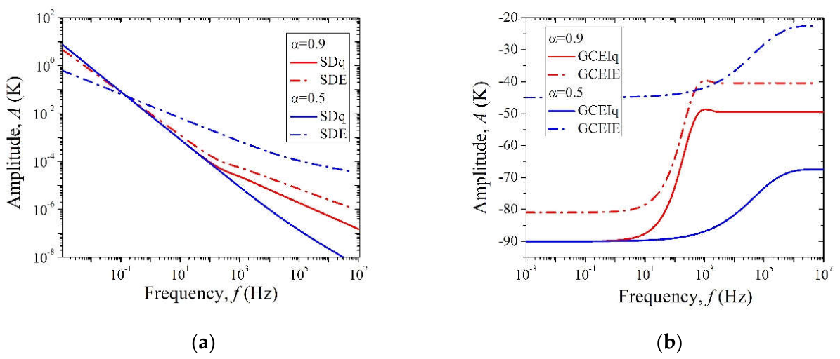
Figure 2.
Temperature variations on the front side of the sample for GCEI: (a) Amplitude characteristics. (b) Phase characteristics.
Figure 2.
Temperature variations on the front side of the sample for GCEI: (a) Amplitude characteristics. (b) Phase characteristics.
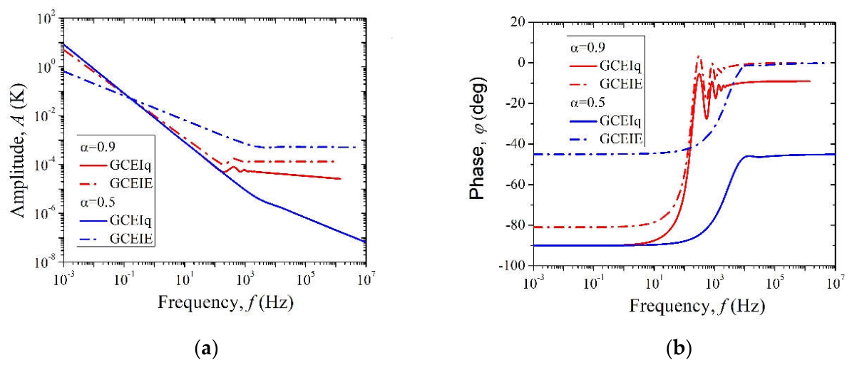
Figure 3.
Classical parabolic and Classical Hyperbolic models: (a) Amplitude characteristic. (b) Phase characteristic.
Figure 3.
Classical parabolic and Classical Hyperbolic models: (a) Amplitude characteristic. (b) Phase characteristic.
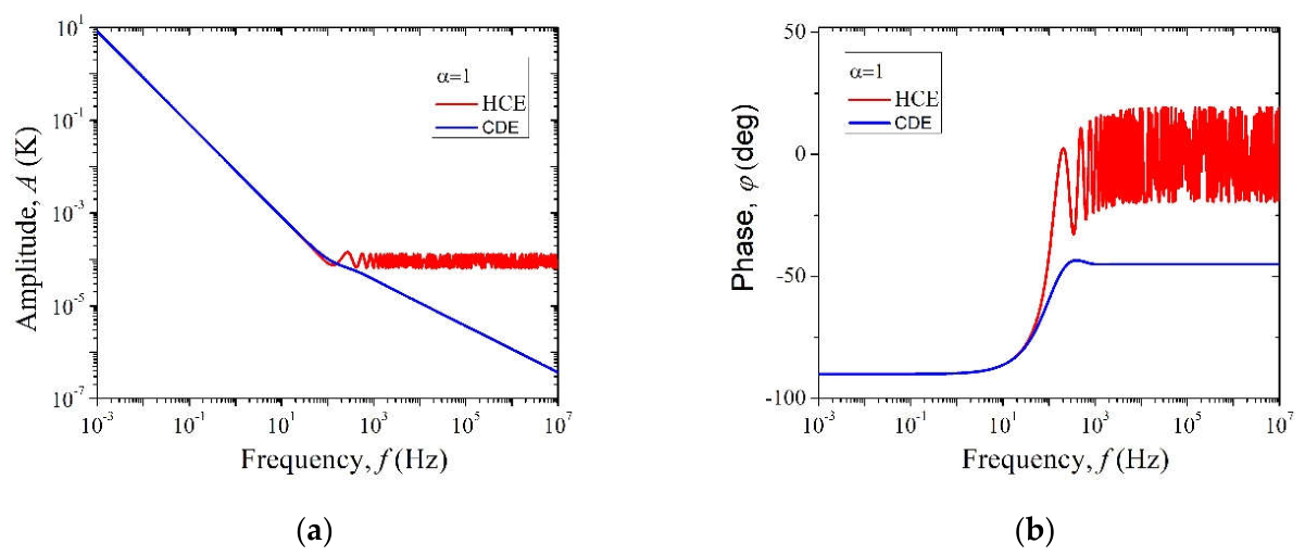

Table 1.
Thermal properties of PA12 [28].
Table 1.
Thermal properties of PA12 [28].
| DT [m2/s] | k [W/(m・K)] | τ [s] |
|---|---|---|
| 1.85·10-7 | 0.23 | 10-3 |
Disclaimer/Publisher’s Note: The statements, opinions and data contained in all publications are solely those of the individual author(s) and contributor(s) and not of MDPI and/or the editor(s). MDPI and/or the editor(s) disclaim responsibility for any injury to people or property resulting from any ideas, methods, instructions or products referred to in the content. |
© 2026 by the authors. Licensee MDPI, Basel, Switzerland. This article is an open access article distributed under the terms and conditions of the Creative Commons Attribution (CC BY) license.
Copyright: This open access article is published under a Creative Commons CC BY 4.0 license, which permit the free download, distribution, and reuse, provided that the author and preprint are cited in any reuse.