

Submitted:
13 September 2026
Posted:
15 September 2026
You are already at the latest version
Abstract
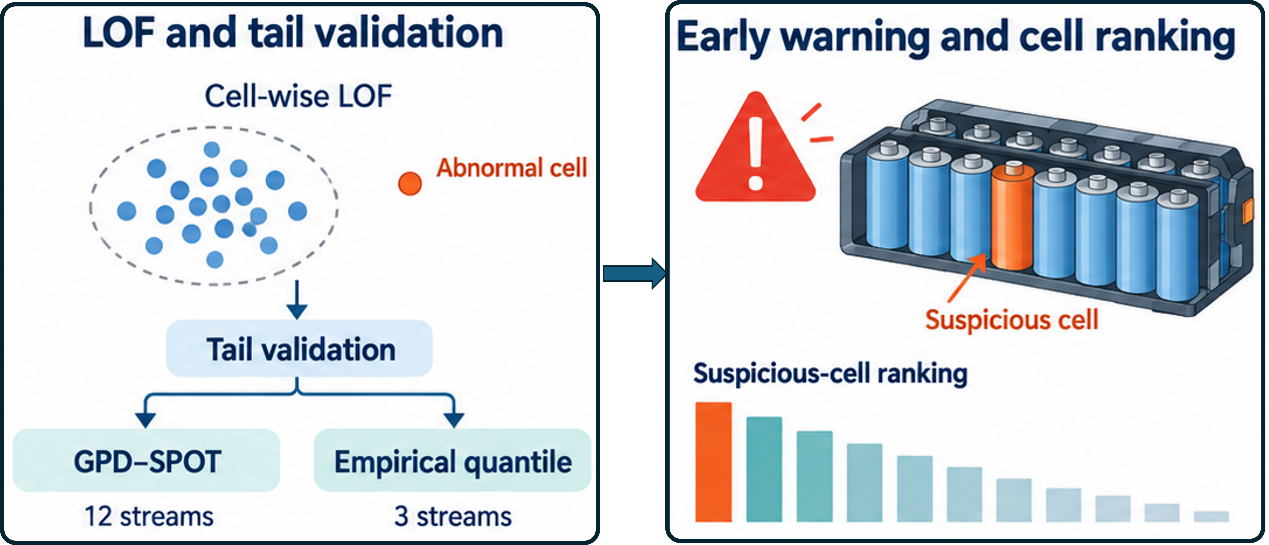
Early fault warning in lithium-ion battery packs is challenged by weak labels and changing operating conditions. This study develops an unsupervised cell-level framework that integrates Local Outlier Factor (LOF) scoring with a validity-gated Streaming Peaks-Over-Threshold (SPOT) rule. Each pack-median-centered voltage trajectory of seven-sample length is characterized by five descriptors, and the maximum cell LOF is logarithmically stabilized as a pack-level anomaly score. The online threshold is estimated via a generalized Pareto distribution (GPD) only when graphical and bootstrap goodness-of-fit diagnostics support the calibrated tail; otherwise, the decision falls back to a higher empirical quantile. Evaluation on real-world vehicles and CH-BatteryGen cases shows that aggregate false-alarm rates are 1.85% and 1.64% for pre-event baselines and normal references at a target risk parameter q = 0.01, respectively. All seven recorded field events are preceded by at least one alarm within 24 hours, yielding a median lead time of 17.39 hours. The tail-validation gate retains GPD-SPOT in 12 of the 15 streams, while the remaining three adopt the empirical fallback. In the three labeled lithium iron phosphate (LFP) cases, the supplied faulty cell ranks first. The framework reports alarm times, suspicious-cell rankings, and the selected thresholding method without fault-labeled training data.
Keywords:
lithium-ion battery
; electric vehicle
; fault warning
; local outlier factor
; extreme-value theory
; adaptive threshold
1. Introduction
Battery safety has become a central concern as transport electrification expands. An emerging cell abnormality may initially produce only a small voltage deviation, even when the underlying process later causes localized current concentration, gas generation, insulation damage, or heat release before conventional protection limits are reached. The practical challenge is to distinguish this early deviation from variations caused by aging, manufacturing dispersion, temperature gradients, and normal load transients [1,2,3,4,5,6]. Laboratory studies isolate these factors by controlling ambient temperature, current profile, and fault intensity. By contrast, fleet telemetry instead contains changing duty cycles, irregular sampling, and missing records. Methods developed under controlled conditions must therefore be evaluated on long-term vehicle records before fleet deployment. Recent real-world studies have used unsupervised fleet learning and drift-aware adaptation to reduce dependence on complete fault labels [7,8]. Graph-guided ensemble learning has further shown that physically informed relationships among battery signals can support fault-risk estimation across heterogeneous vehicle fleets [9]. These studies extend data-driven diagnosis from controlled datasets to field operation.
Voltage is particularly useful because it is routinely measured for every series-connected cell and directly reflects electrical imbalance. The diagnostic meaning of a voltage deviation depends on the operating condition. Generally, resistance growth is often most visible at high current, capacity loss becomes clearer near steep open-circuit-voltage regions or state-of-charge limits, and self-discharge can remain visible as a persistent rest-voltage offset. Internal short circuits, connection faults, overdischarge, and thermal faults can produce related voltage signatures during their early stages [10,11,12,13,14,15,16,17,18,19]. Chemistry also affects signal visibility. The broad voltage plateau of lithium iron phosphate (LFP) cells can reduce separation over part of the usable state-of-charge range, whereas nickel-cobalt-manganese (NCM) cells may show a stronger voltage response to the same capacity mismatch. Complementary sensing studies have broadened the available warning evidence. Online electrochemical impedance spectroscopy has identified impedance features that precede thermal runaway under thermal abuse [20], while expansion-force monitoring has revealed early mechanical signatures under different preload conditions [21]. These results suggest that cell-voltage screening, electrochemical measurements, and mechanical signals can provide complementary evidence for battery safety assessment. In this study, voltage is used for statistical warning and cell ranking, while current and state of charge (SOC) provide post-decision context.
Conventional battery-management systems typically rely on absolute voltage, temperature, current, and insulation thresholds. These thresholds provide transparent protection when a measured quantity crosses a defined limit. Model-based approaches supplement them by forming residuals between measured and estimated responses. Equivalent-circuit, electrochemical, and thermal models have diagnosed internal short circuits, sensor bias, resistance changes, and abnormal heat generation [12,13,14,15,16,17,18]. Long-term feature-residual methods and hybrid observers combine model structure with data-driven adaptation [19,22,23,24]. Cloud-based SOC monitoring extends this analysis to fleet data [25]. Physics-informed neural networks have linked electrode-level degradation to measurable responses [26], while scalable on-road learning has improved health estimation across vehicle types and chemistries [27].
Supervised learning has improved discrimination among known battery fault categories. Support-vector machines, recurrent networks, variational autoencoders, multiscale neural networks, and transfer-learning models have been applied to battery fault recognition [28,29,30,31,32]. Dynamical deep learning has shown that temporal information can improve diagnosis [33], while data aggregation, augmentation, physics-based generation, and imbalance-aware learning expand the available training distributions [34,35]. Deep learning has also identified lithium-plating-type manufacturing defects from formation and capacity-grading records [36], and attention-based impedance models have quantified degradation modes from frequency-dependent responses [37]. These methods are effective when representative labels are available. Field maintenance records, however, usually indicate the fault-confirmation time rather than fault onset, and alarm flags may be delayed or repeated. Such labels support event-time warning and limited cell localization more directly than record-level fault classification.
Unsupervised diagnosis complements these supervised advances by reducing the need to define every potential failure mode in advance. Most cells in a healthy pack behave coherently, so a cell that departs from the local pack population can be identified without assigning a fault class. Local Outlier Factor (LOF) is well suited to this task because it compares local densities rather than imposing one global distance threshold [38,39,40]. LOF-based voltage methods and their extensions have combined local density with dimensionless indicators, fuzzy matrices, signal decomposition, mutual information, and related descriptors [38,39,41,42,43,44,45]. These studies have established a clear cell-level interpretation in which a high score reflects increasing isolation from neighboring cell trajectories. Online deployment requires a thresholding rule that converts cell-level LOF evidence into alarms while accounting for changes in operating regime, sampling density, and healthy-cell dispersion.
Adaptive thresholds convert anomaly scores into alarms while allowing the reference distribution to change over time. Sliding-distance statistics, empirical distribution functions, information entropy, and fuzzy rules have been used to track changes in battery data distributions [46,47,48,49,50]. Extreme-value theory (EVT) models the upper tail of the anomaly-score distribution. Li and Ma combined LOF with a generalized Pareto distribution (GPD) tail model for multi-scenario battery warning [51], and Streaming Peaks-Over-Threshold (SPOT) enabled online tail updating [52]. The anomaly score measures how strongly the current cell pattern differs from the historical observations that did not trigger alarms. The tail model then determines whether that score exceeds the specified upper-tail risk level. Separating these two calculations makes the alarm rule explicit and allows the risk parameter to control threshold stringency.
Recent interpretable diagnostic methods derive information beyond a binary alarm. Enhanced voltage entropy links connection degradation to changes in cell dispersion [41], while mutual information quantifies loss of coherence among cells [42]. Multi-feature clustering and unsupervised scoring combine several signal descriptors [11]. Canonical-variate and autoencoder models form compact latent representations [30,49], and relative-density indices quantify cell inconsistency without a fixed physical model [50]. Maintenance-oriented frameworks additionally estimate where inspection should begin and how urgently action is required [53,54,55]. Following this direction, the present workflow retains the cell-level scores, records the thresholding method, reports a continuous warning index, and quantifies voltage separation under current, SOC, and rest conditions.
The reported alarm rate depends on several implementation choices, including the calibration interval, preliminary tail quantile, SPOT risk parameter, feature normalization, cell-score aggregation, threshold-update rule, and number of windows produced by resampling. The CH-BatteryGen (hereafter CH) dataset provides broad chemistry and fault coverage [56]. Statistics derived after equal-point cycle resampling describe a different time base from statistics derived from the complete variable-length sequence, so the two should be reported separately. Production vehicle data require additional provenance checks because telemetry logs may contain timestamp shifts, partial records, or duplicate files. A duplicate file changes the effective size of the reference cohort, and an undocumented event-time shift changes the calculated warning lead time. Section 2 therefore reports the vehicle identities, source event times, evaluation denominators, and definitions of all derived variables.
In this work, we propose a cell-wise LOF–SPOT warning workflow to detect anomalies in weakly labeled battery-pack telemetry. Five descriptors represent the median-centered voltage trajectory of each cell in a short moving window. The descriptors are normalized across cells within the same window before LOF is calculated. A monotonic logarithmic transform converts the maximum cell LOF into a pack score while preserving score order and reducing the influence of near-singular local-density estimates. SPOT supplies the online upper-tail threshold. A state of safety (SOS) index represents the score exceedance [57], and the cell scores rank cells for inspection. Current coupling, low-state-of-charge amplification, and rest persistence are calculated after the alarm decision to identify whether voltage separation is stronger under load, at low SOC, or during rest.
The study makes four contributions. First, it specifies the complete scoring and threshold-update rules, including feature normalization, neighborhood size (), pack aggregation, calibration length, preliminary tail level, risk probability, and treatment of tail observations. Second, it uses unique vehicle identities and event times taken directly from the source files, allowing the false-alarm denominators and lead times to be reconstructed. Third, event-level performance is reported separately from window-level classification. An event counts as warned if at least one alarm occurs during the preceding 24 h, whereas precision and recall use the complete ±24-h event-label interval. Fourth, parameter robustness is examined across risk probability, window length (), and LOF neighborhood size. The sensitivity analysis reports how these settings change event coverage, false-alarm rate, cell localization, and latency.
2. Data and Parameter Settings
2.1. Data Composition and Analytical Roles
The framework was evaluated using two complementary data sources. The first source was a screened real-world electric-vehicle cohort containing seven event-labeled vehicles and two independent normal vehicles. Event times were read directly from recorded alarm bits or supplied fault-time files without any manual time shift. The second source was CH, from which six chemistry-fault cases were processed using the same feature-construction and thresholding rules. Three LFP cases included supplied faulty-cell labels, allowing cell localization to be evaluated directly. Each selected CH charge or discharge segment was resampled to 60 points, so all reported CH statistics use an equal-point segment time base. Field records were used to calculate event coverage and warning lead time. The CH cases were used to compare chemistry-fault combinations and evaluate cell localization.
The two sources were not combined into one analysis population. The same online rule was applied to every field vehicle. Evaluation reported the pre-event baseline false-alarm rate and whether at least one alarm occurred during the 24 h before each source-recorded event. For the six CH cases, evaluation reported alarm rates across two chemistries and three fault types and tested top-one cell localization in the three labeled LFP cases. The two normal vehicles provide an independent false-alarm reference outside the event-labeled cohort. Each CH stream is a selected fault case, so its alarm rate is reported as a case-level result rather than a field-prevalence estimate. Table 1 summarizes the composition and analytical role of each source. Table 2 traces every derived quantity to its underlying records. Stream-level score counts, calibration sizes, and evaluation denominators are reported in Supplementary Table S1. The audited data-integrity and reporting rules are summarized in Supplementary Table S2, including the exclusion of duplicate car22 records, event-time provenance, LFP cell labels, segment-internal CH windowing, monitoring denominators, and threshold-update exclusions.
2.2. Field-Vehicle Data and Event-Time Provenance
The field data consist of timestamped measurements of current, state of charge (SOC), alarm status, and individual cell voltages. Timestamps were processed according to the source format. For comma-separated-value (CSV) files, the acquisition-time field supplied the timestamps, and the event time was defined as the earliest voltage-related bit-64 alarm. For spreadsheet records, the event time was read directly from the corresponding fault-time file without applying an offset. The storage and vehicle-operation records were joined by nearest-timestamp matching within a two-second tolerance. Each event vehicle contributed data from seven days before to one day after its source event. The two normal vehicles were evaluated over an eight-day interval ending on 31 October 2022. All field streams were sorted chronologically. When a timestamp occurred more than once, only its last record was retained. The data were then resampled to a five-minute grid using the last available observation in each bin. A voltage vector was accepted only when its length matched the modal cell count for that vehicle. Empty five-minute bins were not imputed because the continuity assessment in Section 3.6 required the original telemetry gaps to be preserved.
The event-labeled dataset consists of car9, car10, car12, car14, car16, car20, and car21. The source times are 14 January 2020 08:56:00, 14 January 2020 08:18:12, 9 September 2022 14:04:58, 5 August 2022 05:06:17, 27 July 2022 17:13:38, 2 June 2022 21:01:02, and 29 October 2022 14:54:08, respectively. These timestamps were used directly in the 24-h pre-event and 24-h post-event evaluation windows. “Lead time” is therefore the elapsed time from the first alarm in the pre-event window to the recorded source event. No correction was made for time zone, maintenance delay, or unobserved fault onset.
2.3. CH Cases and Resampled Quantities
Six CH cases were selected to cover high resistance, low capacity, and self-discharge in LFP and NCM packs. Each case contributed twenty charge or discharge segments, except NCM self-discharge vin_34, which contained sixteen valid segments. Numerical channels labeled VOLT (voltage) formed the cell-voltage matrix. For a segment with valid rows, sixty records were selected at , . Charge and discharge segments were ordered by cycle number, with charge preceding discharge within a cycle.
Each sixty-record segment was windowed separately. A seven-sample window produced 54 scores per segment, and no window contained records from two segments. Each twenty-segment case contained 1,080 score windows, of which 216 formed the first 20% calibration block and 864 formed the monitoring block. The sixteen-segment NCM self-discharge case contained 864 score windows, 172 calibration windows, and 692 monitoring windows. Keeping the segments separate excludes 6(S−1) cross-segment windows, where S is the number of segments in the case, otherwise, combining the end of one operating segment with the beginning of the next.
Voltage spread was calculated at each resampled record before windowing as . The spreads from all selected segments in a case were pooled. The 95th-percentile (P95) spread uses the following linear empirical quantile. If the values are ordered as , , and , the reported P95 spread is . The statistic describes upper-end dispersion. Approximately 5% of the equally weighted resampled records have a larger spread.
P95 spread does not enter the LOF features, SPOT fit, alarm decision, SOS calculation, or cell ranking. It is reported only to describe the magnitude of cell-to-cell voltage separation. Equal-point resampling gives every segment the same statistical weight. Therefore, the reported values are not percentiles of every row in the full variable-length vehicle-identification-number (VIN) archive. Comparison with raw-record P95 values is valid only when both calculations use the same segment-weighting rule. The LFP fault-detail file supplied cell 5 for high-resistance vin_60, cell 26 for low-capacity vin_71, and cell 124 for self-discharge vin_1. No ground-truth cell number was supplied for the selected NCM cases.
2.4. Parameter Specification and Selection Rationale
Table 3 lists all numerical settings. The same settings are used for every case, except that the calibration interval is defined differently when the data have a different time base. Event labels were not used to fit or tune the tail model. The two structural parameters control different parts of the calculation. Window length determines how many consecutive records form each cell trajectory. The LOF neighborhood size determines how many nearby cell-feature vectors enter the local-density comparison. The SPOT parameter is the target probability of exceeding the upper-tail threshold. A larger value generally lowers the threshold and produces more alarms, whereas a smaller value produces fewer alarms. The preliminary tail level is calculated from the calibration size so that every fit begins with 20 strict exceedances (scores strictly above the preliminary threshold). A GPD is used only when calibration-stage graphical and bootstrap diagnostics support the fitted tail. No setting was adjusted for an individual vehicle, chemistry, or fault type.
The window length was selected before the alarm-rate analysis using a prespecified three-part rule. First, a candidate setting was retained only if it ranked the supplied faulty cell first in each of the three labeled LFP cases. Second, localization was evaluated without SPOT. Cell-wise LOF evidence was averaged over all windows that remained within a segment, which removed any influence from calibration length or segment order. For a labeled case , denotes the supplied faulty-cell label. The mean evidence of that cell is , and the largest mean evidence among the remaining cells is . Their relative separation is . The selection statistic is the mean of across the three labeled LFP cases. Third, when two settings produced similar localization, the shorter window was preferred because it introduced less delay.
To quantify the trade-off between noise suppression and latency, slope variance was calculated under a simple reference model. For a -point equally spaced window with independent homoscedastic voltage noise of variance , the least-squares slope variance is . This expression is used only as a common analytical reference for comparing window sizes; it does not assert that field-voltage noise is homoscedastic. Applying the three selection criteria led to , which was fixed before the alarm-rate analysis and used for every field and CH case. Section 4.6 reports the quantitative window-size results.
The LOF neighborhood size was set to and capped at , where is the number of valid cells. Candidate values of 15, 20, and 25 were examined. At and , all three labeled LFP fault cells remained first-ranked. At , the first-ranked cell in the high-resistance case changed from cell 5 to cell 24, reducing the top-one result from three cases to two. The selected value preserved all three top-one localization results while using more neighboring cells than the smaller candidate setting. Feature-wise z-score normalization gives the five descriptors the same scale within each window. After centering, a feature is set to zero for every cell if its across-cell standard deviation is below , which prevents division by a numerical zero.
A fixed 98th-percentile preliminary tail was rejected because it left only four to twelve calibration excesses in the available streams and produced boundary estimates that could not support a stable goodness-of-fit assessment. Let denote the number of calibration scores and the target number of excesses. The probability is , with a lower guard of 0.80; is the empirical quantile. In the present data ranges from 0.8837 to 0.9653 and every stream contributes exactly 20 strict calibration excesses.
For each calibration tail, GPD adequacy is assessed by the empirical survival function, the mean-excess curve, and GPD quantile–quantile (Q–Q) and probability–probability (P–P) plots. Cramér–von Mises (CvM) and Anderson–Darling (AD) statistics are calibrated by 500 parametric bootstrap samples in which the GPD is refitted. GPD-SPOT is used only when both bootstrap p-values are at least 0.05 and the shape estimation remains below the upper optimization bound. Otherwise, the online threshold is the higher empirical quantile of accepted history. Alarm observations are not used to update the threshold in either approach.
The tested tail-risk settings were , 0.010, and 0.020. The selection criterion considered the number of recorded events with at least one pre-event alarm and the number of false alarms per monitored baseline window. The final setting was the smallest tested value that produced a pre-event alarm for all seven recorded events. Section 4.6 reports the resulting false-alarm rates and lead times. The realized false-alarm rate does not have to equal because is a target upper-tail probability and successive seven-point windows overlap in six records. This overlap can cluster alarms in time.
Alarm observations were excluded from all threshold updates. Under GPD-SPOT, a non-alarm score above is added to the excess sample and the GPD parameters are refitted; a score at or below increases the number of accepted observations. Under the empirical-quantile method, every non-alarm score is added to the accepted history and the higher empirical quantile is recalculated. Thus, remains the target upper-tail probability under both thresholding methods. GPD-based extrapolation is used only when the calibration diagnostics support the fitted tail.
3. Methodology
The proposed method uses only cell-voltage records and does not require fault-labeled training data or an electrochemical model. Its calculation has three stages. First, LOF compares each cell trajectory with the other cells in the same window. Second, the maximum cell LOF is converted into a pack score. Third, calibration diagnostics select either a GPD-SPOT threshold or an empirical-quantile threshold for that stream. Figure 1 presents the complete calculation order and online update rule from the voltage matrix to the alarm, SOS value, and suspicious-cell ranking. Only non-alarm scores update the threshold, preventing detected anomalies from raising the threshold applied to later observations. For CH data, features are calculated separately within each resampled segment. The score and threshold sequences are then concatenated in fixed cycle order, without constructing voltage windows across segment boundaries.
3.1. Median-Centered Cell-Window Features
Let denote the voltage of cell at record , and let be the number of valid cells. The common pack-level voltage variation is removed at each record by subtracting the cell-voltage median. Median centering retains relative cell behavior and is less sensitive than the mean to a single extreme cell, as shown below.
For a window ending at with length , the trajectory is represented by five features, namely mean, population standard deviation, terminal value, least-squares slope, and range. The main analysis uses ; and 8 form the direct local audit, and and 9 form the broader sensitivity sweep. With and , the features are
The vector contains five measurements of the cell trajectory: sustained offset, short-term fluctuation, terminal separation, linear trend, and total excursion. For each feature , normalization is performed across the cells of the same window, with denoting the across-cell standard deviation, as shown below.
If the across-cell standard deviation is below for a feature, the normalized feature is set to zero for all cells. This within-window normalization compares cells on a common dimensionless scale without using future windows.
Every CH analysis keeps the sixty-record segments separate during feature construction. For labeled case , let denote the set of windows that remain within a segment. The threshold-independent mean LOF evidence for cell is . With denoting the supplied faulty-cell label, define as the evidence of the labeled cell and as the largest mean evidence among the cells without a supplied fault label. The window-size audit uses the relative separation margin , averaged across the three labeled LFP cases. A larger positive value indicates clearer separation between the supplied faulty cell and the strongest alternative. The main CH analysis also forms windows within individual segments. For cell ranking, evidence is averaged over alarm windows, or over all monitoring windows if no alarm occurs, as defined in Section 3.4.
3.2. Cell-Wise LOF and Pack-Score Construction
LOF is evaluated among the cell-feature vectors in one window [38,39,40,43]. Let be the nearest cells under Euclidean distance and the distance from to its th neighbor. The reachability distance prevents a very small pairwise distance from dominating the local density, as shown below.
The local reachability density (lrd) is
The local outlier factor is
A LOF value near unity means that a cell has a local density similar to those of its neighboring cells, whereas a larger value denotes a stronger local deviation. The pack score uses the maximum cell LOF so that one strongly deviating cell can trigger an alarm. The logarithmic transform reduces the influence of near-singular local densities without changing score order, as shown below.
Quantized voltages can produce identical cell-feature vectors and nearly singular local densities. The logarithm limits the resulting pack-score peaks without changing their order. The logarithm limits the resulting peaks without assigning a physical unit to the pack score. Thresholds are fitted separately for each stream, and cell scores are compared only within the same case.
3.3. SPOT Upper-Tail Threshold
For calibration scores , the preliminary tail level is selected by
The calibration-size rule retains 20 calibration excesses in every stream [58,59,60]. Using a fixed number of excesses supports direct comparison of graphical and bootstrap diagnostics across streams. The fixed-count approach replaces the earlier 98th-percentile rule, which was too sparse for the shortest calibration series. The conditional excesses are fitted with a GPD only when the adequacy tests support that model. The fitting conditions are given below.
where is the scale, is the shape, and is the number of strict calibration scores above . Maximum-likelihood fitting constrains to . For every candidate tail, the empirical survival function is compared with . The mean-excess function is estimated as ; approximate pointwise intervals use . A stable or approximately linear mean-excess curve supports, but does not by itself establish, GPD adequacy. GPD Q–Q and P–P plots examine the tail magnitudes and fitted probabilities, respectively [58,59].
with the continuous limit as approaches zero. Cramér–von Mises and Anderson–Darling statistics are calculated from the probability-integral-transformed excesses. Their p-values are obtained from 500 GPD samples of size , with and refitted in every replicate [60]. GPD-SPOT is selected only when both p-values are at least 0.05 and the fitted shape parameter remains below the upper optimization bound. A fit that terminates at that bound is rejected because its tail shape is not reliably identified.
If this gate fails, denotes the calibration scores plus all accepted non-alarm monitoring scores before , and the fallback threshold is
The higher empirical quantile prevents interpolation above an observed order statistic. Under either thresholding method, denotes an alarm, and that score is excluded from subsequent threshold updates. Under GPD-SPOT, each accepted non-alarm score above is added to the excess sample. Under the empirical-quantile method, every accepted non-alarm score is added to . Successive seven-point windows share six records, so the diagnostics assess the distribution of tail magnitudes but not temporal independence. A seven-run extremal index quantifies this clustering. The empirical false-alarm rate is reported separately to evaluate threshold behavior on the monitored records.
3.4. SOS, Cell Ranking, and Operating Context
Following the graded reporting concept in [57], the contemporaneous score-threshold gap is converted to a bounded SOS warning index. The index decreases as the score moves farther above the threshold and is defined as follows.
The scale is fixed at 1 before analyzing any outcome; it is not tuned by vehicle, chemistry, or fault type. Every non-alarm window has , while a larger score-threshold gap produces a lower SOS. With the alarm fraction and the mean SOS among alarm windows , the all-window mean satisfies
Equation (13a) shows that sparse alarms keep the all-window mean close to 100 because every non-alarm window contributes 100. Results are consequently reported as alarm count and rate together with the alarm-only median, interquartile range (IQR), minimum, and proportions below 90, 75, and 50. Values below 0.01 arise from exponential numerical saturation at large score-threshold gaps and are reported as <0.01. These values are purely numerical and should not be interpreted as zero physical safety.
To rank cells for inspection, let be the set of monitoring windows that triggered alarms. Cell evidence is
and cells are ordered by decreasing . If is empty, evidence is averaged over all monitoring windows instead. For visualization, the evidence values in each case are divided by their case-specific maximum. This normalization does not change the rank or the selected cell.
After the alarm decision, three contextual indicators are calculated from . Current coupling is . Low-state-of-charge amplification is when both SOC regions are available. Rest persistence is . These ratios describe the operating conditions under which pack voltage spread is larger and do not affect threshold adaptation or alarm generation. A high current correlation means that the spread increases with current magnitude. A high low-SOC ratio means that the average spread is larger below 30% SOC than above 70% SOC. A high rest-persistence ratio means that much of the average spread remains when the current magnitude is below 5 A.
3.5. Evaluation Definitions
For an event vehicle with a recorded event time T, the event-label interval is . The ±24-h interval is referred to as the ‘weak event window’ because it broadly labels records near the event time without identifying the true fault onset. Monitoring records earlier than form the pre-event baseline. The false-alarm rate is the number of alarms in that baseline divided by the number of monitored baseline windows. An event is counted as having a pre-event warning when at least one alarm occurs in . Lead time is measured from the first such alarm to . Precision and recall treat every record in the complete ±24-h interval as positive because the source data do not identify the true fault-onset time. Precision and recall are therefore window-level results for the broad ±24-h label, not estimates of the number of physically faulty records. Aggregate rates are calculated by summing alarms and monitored windows across vehicles before division; they are not arithmetic means of vehicle-level percentages. For each CH case, alarm rate is the number of alarms divided by the number of monitoring windows. Localization is top-one correct when the first-ranked cell matches the supplied fault-cell label.
3.6. Pre-Event Voltage-Morphology Audit
A separate retrospective audit examined whether the voltage records provided sufficient evidence of progressive-like or abrupt-like pre-event changes. It was performed after the warning analysis and was not used to select or tune any detector parameter. For each source event time T, the observed five-minute records in were retained without filling empty bins. At each record, low-side and high-side residuals were calculated relative to the contemporaneous pack median as follows.
A positive means that cell lies below the pack median, whereas a positive means that it lies above the median. The candidate cell and direction were selected by the largest cell-wise 95th-percentile residual in the final two hours. The early and final-two-hour levels were calculated from the original five-minute residual records over to h and to , respectively. Temporal completeness and the maximum gap were also calculated from the original five-minute records. For trend testing, the selected residual was aggregated into ten-minute medians using bins anchored at . This aggregation reduces sensitivity to irregular record density while preserving genuine telemetry gaps. The robust trend estimate is the Theil-Sen median slope [61], which is defined as follows.
A progressive-like morphology required , a 95% confidence interval entirely above zero, a two-sided Mann-Kendall trend-test [62], and no unresolved telemetry gap spanning the increase. An abrupt-like morphology required a positive ten-minute change that accounted for at least 50% of all positive change and was bracketed by observations no more than 30 min apart. Cases that failed these evidential requirements were classified as indeterminate rather than being assigned a fault mechanism. The audit does not assign a physical fault mechanism. Distinguishing capacity fade, internal short circuit, contact resistance, or sensor error requires corroborating current, temperature, resistance, capacity, or inspection evidence.
4. Results and Discussion
4.1. Reliability Checks and Analysis Population
After identity and timing audits, the field population contains 6,557 pre-event baseline windows across seven event-labeled vehicles and 2,498 monitoring windows across two independent normal vehicles. The event-labeled group produced 121 baseline alarms, and the normal group produced 41. Dividing these aggregate alarm counts by their corresponding window counts gives false-alarm rates of 1.845% and 1.641%, respectively. Table 4 and Table 5 report the vehicle-level and aggregate field results, respectively.
For CH, segment-internal windowing produces 1,080 score windows for each twenty-segment case and 864 for the sixteen-segment case. Segment-internal windowing removes 114 artificial windows from each twenty-segment sequence and 90 from the sixteen-segment sequence. The resulting monitoring denominators are 864 and 692. P95 spread remains based on sixty resampled voltage rows per segment and is therefore unaffected by the window-boundary correction. All field and CH cases were processed using the same scoring, thresholding, alarm, SOS, and cell-ranking rules. For example, the LFP high-resistance alarm rate is .
4.2. Online Threshold Behavior
As shown in Figure 2, the stabilized pack score (blue line) is compared with its online threshold (orange line) on the same score-window axis. The gray dashed vertical line marks the end of calibration; only points to its right are evaluated for alarms. A red point marks a score above the threshold. Panels (a) and (b) show field streams. Panels (c) and (d) show CH cases in which a small number of score peaks lie far above most observations. The first three panels use GPD-SPOT. Panel (d) uses the empirical threshold because the NCM low-capacity calibration tail fails both goodness-of-fit tests.
Car18 produces 12 alarms among 889 monitoring windows (1.35%). Car10 produces 15 alarms among 419 pre-event baseline windows and six alarms within ±24 h of the recorded event. One of these six alarms occurs 0.053 h before the recorded event time. This alarm satisfies the prespecified rule that an event is warned when at least one alarm occurs in the preceding 24 h. The 0.053-h interval is nevertheless too short to represent useful advance notice, so it is reported separately from the other six lead times, all longer than 10 h.
The two CH panels illustrate different threshold decisions. The LFP high-resistance stream contains isolated score spikes, but its calibration excesses pass the stated GPD tests. In the NCM low-capacity stream, most scores form a compact group and several peaks are much larger because some LOF density estimates are nearly singular. The calibration tests reject a single GPD for this tail, so the online detector uses the empirical threshold. In both cases, the alarm rate equals the number of threshold exceedances divided by the number of monitoring windows. P95 spread separately reports the amplitude of cell-to-cell voltage separation.
4.3. Cross-Chemistry and Fault-Type Alarm Rates
As shown in Figure 3, blue bars represent the three LFP cases, and orange bars represent the three NCM cases. Bar height and the number printed above it give the monitoring alarm rate; diagonal hatching marks a case for which the calibration GPD was rejected and the empirical threshold was used. Table 6 reports the corresponding alarm counts, monitoring denominators, alarm rates, all-window SOS values, minimum SOS values, and resampled P95 voltage spreads. Alarm rates are 1.74%, 2.31%, and 0.46% for LFP high resistance, low capacity, and self-discharge, respectively, giving a mean of 1.50%. The corresponding NCM rates are 0.81%, 3.47%, and 1.45%, giving a mean of 1.91%. The chemistry contrast varies by fault type. NCM is lower for high resistance, higher for low capacity, and intermediate for self-discharge. NCM low capacity accounts for most of the 0.40-percentage-point difference between the chemistry means.
NCM low-capacity vin_71 has 30 alarms among 864 monitoring windows, compared with for LFP low-capacity vin_71. The NCM rate is therefore 1.16 percentage points higher, and the rate ratio is 1.50. In this matched pair, the NCM stream exceeds its own adaptive threshold more often than the LFP stream. The result is based on one matched pair and does not establish a general chemistry-dependent difference in fault detectability.
4.4. Faulty-Cell Localization
Figure 4 presents the cell-level localization profiles, with cell number on the horizontal axis and normalized mean LOF evidence on the vertical axis. The blue line shows the evidence for every cell. The red marker identifies the first-ranked cell, and the orange dashed line identifies the supplied faulty cell when an LFP label is available. Panels (a)–(c) directly compare the first-ranked cell with the supplied LFP label. Panels (d)–(f) show only the first-ranked NCM cells because no NCM reference-cell labels were provided. All three supplied LFP fault cells are ranked first. They are cell 5 for high-resistance vin_60, cell 26 for low-capacity vin_71, and cell 124 for self-discharge vin_1. In the labeled panels, overlap between the red marker and orange line denotes correct localization. The vertical gap between the leading peak and the highest remaining peak shows how clearly the first-ranked cell is separated from the other cells. Table 7 lists these cell ranks together with the corresponding operating-condition indicators.
Localization separation differs among the six cases. The LFP high-resistance profile contains several large secondary peaks, so its leading cell is less clearly separated from the remaining cells. The LFP low-capacity and self-discharge profiles each contain one more dominant peak. A well-separated leading peak identifies a specific cell for inspection, whereas a flatter profile leaves several plausible cells as candidates for further investigation. In the NCM cases, cells 53, 18, and 61 rank first for high resistance, low capacity, and self-discharge, respectively. These cells are algorithmic inspection targets rather than confirmed faulty cells because the fault-detail file contains no NCM cell labels.
4.5. Operating-Condition Indicators
As shown in Figure 5, the six CH cases are arranged by row and the three operating-condition indicators by column. Color is used to compare cases within one indicator, not to compare the numerical scales of different indicators. Current coupling is high in both high-resistance cases, with values of 0.98 for LFP and 0.97 for NCM. Their rest-persistence values are much lower at 0.18 and 0.16. Low-SOC amplification is largest in LFP low capacity (2.60), followed by NCM self-discharge (1.96) and LFP self-discharge (1.75). The indicator values identify whether voltage separation is most visible under load, at low SOC, or during rest. The indicators are calculated after detection and do not enter the alarm calculation.
The resampled P95 voltage spreads are 132.15, 26.05, and 12.00 mV for LFP high resistance, low capacity, and self-discharge, and 78.00, 97.00, and 45.00 mV for the corresponding NCM cases. These values were computed directly from the sixty-point segment rule in Section 2.3. For example, each twenty-segment case contributes spreads, so P95 lies between the 1,140th and 1,141st ordered values under the stated linear interpolation. The NCM self-discharge case contributes 960 spreads because only sixteen segments were valid.
P95 reports upper-end voltage imbalance without being determined by a single maximum; it does not measure alarm performance. LFP high-resistance vin_60 has the largest P95 spread (132.15 mV) and an alarm rate of 1.74%, whereas LFP low-capacity vin_71 has a smaller P95 spread (26.05 mV) but a higher alarm rate of 2.31%. NCM low-capacity vin_71 combines a P95 spread of 97.00 mV with the highest alarm rate, 3.47%. A larger P95 spread therefore does not necessarily produce a higher alarm rate because the alarm rate depends on threshold exceedances rather than spread magnitude alone.
4.6. Sensitivity and Robustness
Figure 6 summarizes the sensitivity of the warning results to the tail-risk parameter . Panel (a) compares aggregate false-alarm rates in the event baselines and independent normal vehicles. Panel (b) shows the number of recorded events with at least one pre-event alarm on the left axis and median lead time on the right axis. Panel (c) compares mean CH alarm rates by chemistry, and panel (d) reports precision and recall under the ±24-h event-label definition. Increasing from 0.005 to 0.010 raises the number of events with a pre-event alarm from five to seven. Over the same change, the event-baseline false-alarm rate rises from 1.13% to 1.85%. Raising further to 0.020 does not increase the number of warned events above seven, but it raises the event-baseline false-alarm rate to 3.45% and the normal-vehicle rate to 2.76%. Therefore, is the smallest tested value that produces a pre-event alarm for all seven recorded events. Table 8 provides the numerical results for all three tested risk settings.
The median lead times are 15.49, 17.39, and 21.74 h at , 0.010, and 0.020, respectively. Across the same range, precision increases from 0.362 to 0.443, and recall under the ±24-h event-label definition increases from 0.013 to 0.056. The mean CH alarm rate rises from 0.85% to 2.58% for LFP and from 1.21% to 2.97% for NCM. A larger lowers the extreme-quantile threshold and increases both pre-event event coverage and false-alarm frequency. Supplementary Table S3 comprises two parts. Table S3a reports the field results for each tested q value, and Table S3b reports the corresponding CH results.
To assess sensitivity to window size, a direct comparison was made among the three settings , 7, and 8. As shown in Figure 7, the window-size comparison is independent of the threshold model. Panel (a) shows the separation margin between the supplied faulty cell and the strongest alternative for each labeled LFP case. A positive margin means that the supplied cell is first-ranked, and the margin remains positive at every tested window size. Panel (b) shows the mean margin across the three labeled cases and reports the top-one result above each bar. Panel (c) shows the analytical slope-variance factor together with the time span at the five-minute field sampling interval. For the three settings, the mean separation margins are 45.82%, 46.22%, and 45.85%, respectively. The corresponding slope-variance factors are 0.05714, 0.03571, and 0.02381, and the corresponding time spans are 25, 30, and 35 min. Moving from six to seven samples reduces the slope variance by 37.5% and slightly increases the mean separation margin. Moving from seven to eight samples reduces the variance further, but it adds five minutes to the window span and slightly lowers the observed mean margin. The setting retained top-one localization, reduced slope variance relative to the six-sample setting, and avoided the additional five-minute span of the eight-sample setting. Supplementary Table S4 lists the case-level labeled-cell margins and top-ranked cells for each window length. Supplementary Table S5 gives the corresponding aggregate window counts, slope-variance factors, mean margins, and top-one results.
Calibration length was not varied in this comparison. Changing the value would alter the tail sample, the number of monitoring windows, and the period in which a pre-event alarm could be observed. Therefore, the main robustness results focus on sensitivity to and window size. Optimizing calibration duration would require a larger prospective cohort in which the available pre-event monitoring period is controlled.
The LOF neighborhood size was kept at for the sensitivity results in Figure 6 and Figure 7. Section 2.4 reports the comparison with and . The sweep was not extended beyond the prespecified values because exact duplicate feature vectors in quantized CH telemetry can destabilize density at values substantially larger than the selected k = 20.
4.7. Calibration-Tail Validation
As shown in Figure 8, the stabilized score is plotted on the horizontal axis and its exceedance probability on the vertical axis. The blue step curve is the empirical calibration survival, the red dashed curve is the unconditional survival implied by the fitted GPD tail, and the orange vertical line is the selected preliminary threshold . Each inset reports the calibration size , the retained excess count , the fitted shape , the CvM and AD bootstrap p-values, and whether the online detector uses GPD-SPOT or the empirical threshold. Agreement between the blue and red curves for scores above supports the fitted tail model. A systematic gap, or an empirical step that the fitted curve does not reproduce, indicates that one GPD does not adequately describe the calibration excesses.
Panels (a) and (b) show close agreement between the fitted tail and empirical steps above the preliminary threshold. Car18 has with CvM and AD . Car10 has , which indicates a bounded tail over the observed range; its CvM and AD p-values are 0.479 and 0.475. Panel (c) is less regular. LFP high resistance has and one excess much larger than the others. The CvM and AD p-values are 0.192 and 0.234, so the tests do not reject the fitted heavy tail. However, the long empirical plateau and only excesses make extrapolation beyond the observed scores uncertain. Panel (d) shows a clear lack of fit for NCM low capacity. Its empirical survival curve contains a long plateau followed by one isolated extreme score, which the fitted GPD cannot reproduce. Both p-values are 0.002. The fitted curve is included only to show this mismatch and is not used for online thresholding; the detector uses the empirical quantile instead. Figure 8 therefore tests a distributional assumption that cannot be judged from the online traces in Figure 2 alone.
As shown in Figure 9(a), the mean excess for car18 varies from approximately 0.050 to 0.075 across the displayed thresholds, with a value of 0.052 at the selected threshold. Car10 shows an overall decrease, reaching 0.080 at the selected threshold (Figure 9(b)). The LFP high-resistance case shows a generally increasing mean excess, with a value of 1.44 at the selected threshold (Figure 9(c)). For NCM low capacity, the curve changes little around the selected threshold but rises sharply at the highest candidate thresholds (Figure 9(d)). In both CH cases, increasing the threshold excludes smaller scores, leaving the mean excess more strongly influenced by the largest observations. The orange markers identify the preliminary thresholds determined by the calibration-size rule in Eq. (11), each retaining 20 strict excesses. The thresholding method follows the goodness-of-fit and shape-parameter criteria in Section 3.3. These criteria retain GPD-SPOT for car18, car10, and LFP high resistance. For NCM low capacity, both bootstrap CvM and AD p-values are 0.002, so the empirical quantile is used, as listed in Supplementary Table S6.
Figure 10 evaluates the fitted tails in two coordinate systems. Panels (a)–(d) are Q–Q plots. The horizontal coordinate is the GPD theoretical excess quantile and the vertical coordinate is the observed excess quantile. Panels (e)–(h) are P–P plots. Empirical cumulative probability is on the horizontal axis and fitted GPD probability is on the vertical axis. The red dashed identity line represents exact agreement. Random scatter around that line is expected for ; curvature, flattening, or one-sided separation indicates that the fitted distribution does not reproduce the observed tail. The field points in panels (a), (b), (e), and (f) remain close to the identity line, apart from modest finite-sample scatter. Panels (c) and (d) each contain one upper-order statistic far above the Q–Q trend. These are observed calibration scores rather than plotting artefacts. Quantized CH voltage creates duplicate or nearly duplicate cell-feature vectors; when one cell separates, its local reachability density can become nearly singular, and the maximum-across-cell LOF retains that isolated peak even after logarithmic stabilization. In panel (c), the fitted positive shape is flexible enough that the bootstrap tests do not reject the heavy tail, although the upper point is influential and the resulting threshold remains uncertain. In panel (d), the gap between the ordinary excesses and the isolated peak is too large for one continuous GPD.
The lack of fit is clearest for NCM low capacity in panel (h). Most fitted probabilities occupy a narrow, nearly horizontal band, while the empirical probabilities span almost the full unit interval. The fitted model therefore assigns similar probabilities to many different empirical ranks and cannot reproduce the combination of a plateau and a separated maximum. Both CvM and AD tests consequently return , and the empirical threshold is used. Across all 15 streams, all nine field tails and three CH tails satisfy the complete set of diagnostic criteria. LFP low capacity, NCM low capacity, and NCM self-discharge fail at least one criterion and use the empirical threshold. Supplementary Table S6 reports the calibration-tail parameter estimates, both bootstrap p-values, and the thresholding method retained for all 15 streams.
The seven-run extremal-index estimates range from 0.10 to 0.55, showing that threshold exceedances are clustered partly because successive windows overlap. The bootstrap tests assess whether the distribution of excess magnitudes is compatible with a GPD. These tests do not assess temporal independence or guarantee that the realized false-alarm rate equals . The aggregate reference false-alarm rates are 1.845% for event baselines and 1.641% for normal vehicles. Their close agreement provides a direct check of detector behavior on reference data.
4.8. SOS Magnitude and Operational Interpretation
As shown in Figure 11, alarm frequency is separated from the magnitude by which alarm scores exceed their thresholds. The corresponding alarm counts, alarm rates, and alarm-only SOS summaries are listed in Table 9. In panels (a) and (b), each dot represents one alarm window. The horizontal line in each box is the median, the box covers the interquartile range (IQR), and the whiskers show the remaining non-outlying values. The label gives the number of alarm windows. Panel (a) compares the pre-event baselines, the ±24-h event-label intervals, and the independent normal vehicles. Panel (b) compares LFP and NCM cases. Panel (c) places alarm rate on the horizontal axis and median alarm-only SOS on the vertical axis. Circles represent GPD-SPOT, and squares represent the empirical threshold. A lower SOS means that an alarm score lies farther above its threshold. Supplementary Table S7 provides the corresponding stream-level all-window and alarm-only SOS summaries.
Among field alarms, the pre-event-baseline SOS median is 93.98 (IQR 90.33–97.62; minimum 72.08), the ±24-h event-label-interval median is 95.96 (IQR 91.15–98.22; minimum 73.48), and the independent-normal-vehicle median is 94.19 (IQR 91.48–97.77; minimum 83.37). The three boxplots overlap substantially, so alarms in the ±24-h event windows do not show systematically larger exceedances than alarms in either reference group.
The CH cases show a wider alarm-only range. The LFP medians are 85.38 for high resistance, 77.71 for low capacity, and 81.04 for self-discharge; their IQRs are 41.39–86.88, 70.57–89.93, and 65.87–94.14. The NCM medians are 69.57, <0.01, and 34.42, with IQRs of 62.24–80.80, <0.01–93.48, and 22.52–64.79. occurs in 4/15, 9/20, and 2/4 LFP alarms and in 4/7, 21/30, and 8/10 NCM alarms. The 21 large gaps between the LOF score and its threshold in NCM low capacity reduce its median alarm-only SOS to <0.01.
Alarm rate reports how often the threshold is exceeded, whereas alarm-only SOS reports the magnitude of those exceedances. NCM high resistance has fewer alarms than LFP high resistance (0.81% versus 1.74%) but a lower median SOS (69.57 versus 85.38), indicating rarer but larger departures. NCM low capacity combines the highest rate (3.47%) with the lowest median, whereas LFP self-discharge combines the lowest rate (0.46%) with a median of 81.04. Across the six CH cases, the Spearman association between alarm rate and median alarm SOS is (). The six-case result shows no statistically significant monotonic association.
All-window mean SOS remains between 97.54 and 99.90 in the CH cases because every non-alarm window equals 100, as shown by Eq. (13a). This mean value is therefore dominated by non-alarm windows and cannot reliably distinguish fault severity. The fixed setting preserves the ordering of score-threshold gaps within each stream but does not make their magnitudes directly comparable across different sampling intervals or thresholding methods.
4.9. Field Warning Performance, Pre-Event Morphology, and Operational Meaning
As listed in Table 4, baseline FAR ranges from 0.61% for car16 to 3.58% for car10. The aggregate event-baseline FAR is 1.845%, which is close to the 1.641% obtained from the independent normal vehicles. The 0.204-percentage-point difference indicates similar reference alarm frequencies in the two cohorts. The realized rates also show that the 0.01 tail-risk setting does not guarantee a 1% false-alarm rate.
Each of the seven recorded field events is preceded by at least one alarm. Lead times are 22.43 h (car9), 0.053 h (car10), 10.83 h (car12), 19.85 h (car14), 17.39 h (car16), 15.43 h (car20), and 21.74 h (car21). The median is 17.39 h. Six lead times exceed 10 h. The car10 alarm occurs almost at the recorded event time and should not be described as useful advance warning. Each lead time is calculated to the source-recorded event time and therefore does not estimate physical fault onset or the rate of preceding voltage change.
Within the event-labeled monitoring data, 91 of 212 alarms occur inside the ±24-h event-label intervals, giving a precision of 0.429. Those intervals contain 3,191 monitored windows, of which only 91 are alarms, giving a recall of 0.029. The event-level and window-level metrics give different results. All seven events are covered, whereas alarms occur in only 2.9% of the broadly labeled windows.
As shown in Figure 12 and listed in Table 10, the independent audit combines voltage-residual trajectories with data-coverage and trend statistics. Each blue marker is the ten-minute median residual of the selected cell relative to the pack median, and the red dashed line marks the source event. Adjacent markers are connected only when they are separated by no more than 30 min. A rising trajectory indicates that the selected cell is becoming more separated from the pack median. A line break marks an interval without observations; no voltage trajectory is inferred across that interval. Each panel has its own vertical scale because the residual ranges differ among vehicles. Table 10 reports coverage, maximum gap, and the early and final-two-hour medians calculated from the original five-minute records. It also reports the Theil-Sen slope and Mann-Kendall p-value calculated from the ten-minute median series in Figure 12. The line breaks in panels (a)–(c) are intentional. The largest gaps between plotted ten-minute bins are 10.00 h for car9, 10.33 h for car10, and 1.17 h for car12. The corresponding maximum gaps between successive valid five-minute records are 10.00, 10.42, and 1.08 h, as listed in Table 10. Connecting points across these intervals would depict voltage behavior that was not observed and could falsely support a progressive-like or abrupt-like classification.
All seven final-window candidates are low-side deviations; none is dominated by a high-side excursion consistent with an observed pre-event overvoltage morphology. Car9 shows the clearest late separation. Cell 10 increases from an early median of 5.00 mV to 18.00 mV in the final two hours, and its final-30-min median is 74.50 mV. However, coverage is only 55.2%, and the apparent rise is separated from the preceding trajectory by a 10.00-h gap. Its Theil-Sen slope is 0.057 mV h−1 (95% confidence interval, -0.044 to 0.250 mV h−1; ), indicating that a sustained progressive trend is not established. Car10 cell 28 increases from 3.00 to 34.00 mV and has a positive slope of 0.378 mV h−1 (95% confidence interval, 0.188-0.625 mV h−1; ). Nevertheless, only 19.1% of the expected records are present and a 10.42-h gap spans the increase. The data therefore do not reveal whether the separation developed gradually within that gap or appeared abruptly.
The remaining five cases do not show a sustained increase toward the recorded event time. For car12, the low-side residual decreases from 39.00 to 15.50 mV, with a slope of -0.816 mV h−1. For car14, it decreases from 18.75 to 10.00 mV, with a slope of -0.344 mV h−1. For car16, it decreases from 23.50 to 16.00 mV, with a slope of -0.282 mV h−1. Each of these three trends has . Car20 remains stable at approximately 10 mV, with mV h−1 and . Car21 is non-monotonic and has no significant trend, with mV h−1 and . None of these five trajectories shows a sustained increase in low-side voltage separation. None contains a sufficiently observed late step to meet the abrupt-like criterion.
None of the seven events meets the prespecified criteria for progressive-like or abrupt-like voltage morphology. The reported lead times therefore locate alarms relative to source event timestamps but do not identify physical fault onset. Near the recorded events in car9 and car10, the selected cells show larger negative voltage deviations from their respective pack medians than in the earlier observed records. Long telemetry gaps separate the earlier and later observations, so the available records cannot show whether these deviations increased gradually or appeared abruptly. More continuous telemetry or maintenance evidence is required to distinguish gradual capacity-related divergence from an abrupt electrical event or a sensing fault.
5. Conclusions
This study developed an unsupervised cell-wise warning method for weakly labeled battery-pack telemetry. The evaluation used verified vehicle identities, source event timestamps, and segment boundaries. Each calibration tail had to pass graphical and bootstrap tests before GPD-SPOT was used. The diagnostics supported GPD-SPOT in all nine field streams and three of the six CH streams; the remaining three CH streams used empirical thresholds. At q = 0.01, aggregate false-alarm rates were 1.85% for the pre-event baselines and 1.64% for the normal-vehicle data. Each of seven recorded field events had at least one alarm in the preceding 24 h, and the median lead time was 17.39 h. However, the car10 alarm occurred only 0.053 h before the recorded event and thus did not provide useful advance notice.
Across the CH cases, mean alarm rates were 1.50% for lithium iron phosphate and 1.91% for nickel-cobalt-manganese batteries. LOF ranked the supplied faulty cells first in all three labeled lithium iron phosphate cases. The selected seven-sample window also reduced slope variance relative to the six-sample setting and avoided the additional five-minute span of the eight-sample setting. Alarm-only SOS summarized the score-threshold gaps among alarm windows. The independent 24 h morphology audit could not classify any event reliably as progressive-like or abrupt-like because long telemetry gaps covered the late voltage separation in car9 and car10, while the other five events showed no sustained pre-event increase. The reported lead times therefore describe the timing of statistical alarms relative to source event timestamps, not the duration of physical fault progression. The framework reports alarm times, ranked cells, and a validated online threshold for inspection prioritization.
Supplementary Materials
The following supporting information can be downloaded at the website of this paper posted on Preprints.org.
Author Contributions
X.Y.: Conceptualization, Investigation, Methodology, Resources, Validation, Writing. Z.Z.: Data curation, Formal analysis, Investigation, Writing. Z.Q.: Conceptualization, Formal analysis, Methodology, Software, Validation. B.L.: Conceptualization, Funding acquisition, Supervision, Writing, Project administration. All authors have read and agreed to the published version of the manuscript.
Funding
This work was supported by Key Research and Development Program of Zhejiang Province (No. 2024C01062).
Data Availability Statement
The analysis used the field-vehicle files, fault-detail workbook, and CH-BatteryGen described in Section 2. The main tables and Supplementary Material provide the complete parameter specification, evaluation denominators, case-level outputs, and sensitivity settings needed to reproduce the reported results. Access to the underlying field data remains subject to the data owner’s conditions.
Conflicts of Interest
The authors declare that they have no known competing financial interests or personal relationships that could have appeared to influence the work reported in this paper.:
References
- Zhao, J.; Feng, X.; Tran, M.-K.; Fowler, M.; Ouyang, M.; Burke, A.F. Battery safety: Fault diagnosis from laboratory to real world. J. Power Sources 2024, 598, 234111. [Google Scholar] [CrossRef]
- Zhao, J.; Liu, M.; Zhang, B.; Wang, X.; Liu, D.; Wang, J.; Bai, P.; Liu, C.; Sun, Y.; Zhu, Y. Review of lithium-ion battery fault features, diagnosis methods, and diagnosis procedures. IEEE Internet Things J. 2024, 11, 18936–18966. [Google Scholar] [CrossRef]
- Yao, L.; Yu, C.; Xiao, Y.; Cui, G.; Fei, Z.; Qu, C. A comprehensive review of lithium-ion battery safety issues and fault diagnosis strategies throughout the entire lifecycle. J. Energy Storage 2025, 136, 118447. [Google Scholar] [CrossRef]
- El-Mahdy, M.H.; El-Gendy, E.M.; Ismael, I.; Saafan, M.M. Advancements in fault diagnosis and fault tolerant control of lithium-ion battery systems for electric vehicles: Theoretical and real-time approaches. J. Energy Storage 2026, 152, 120794. [Google Scholar] [CrossRef]
- Polat, K.; Daldal, N.; Zaib, M.; Arabaci, B. Enhancing the safety and reliability of electric vehicles through effective battery fault diagnosis: A systematic review. Comput. Electr. Eng. 2026, 129, 110831. [Google Scholar] [CrossRef]
- Xiong, R.; Sun, W.; Yu, Q.; Sun, F. Research progress, challenges and prospects of fault diagnosis on battery system of electric vehicles. Appl. Energy 2020, 279, 115855. [Google Scholar] [CrossRef]
- Yu, Q.; Yang, Y.; Tang, A.; Wu, Z.; Xu, Y.; Shen, W.; Zhou, F. Unsupervised learning for lithium-ion batteries fault diagnosis and thermal runaway early warning in real-world electric vehicles. J. Energy Storage 2025, 109, 115194. [Google Scholar] [CrossRef]
- Peng, X.; Duan, S.; Sankavaram, C.; Jin, X. Unsupervised adaptive fleet battery pack fault diagnosis with concept drift under evolving environment. IEEE Trans. Autom. Sci. Eng. 2024, 21, 2276–2291. [Google Scholar] [CrossRef]
- Zhang, C.; Li, S.; Du, J.; Zhang, L.; Luo, W.; Jiang, Y. Graph-guided fault detection for multi-type lithium-ion batteries in realistic electric vehicles optimized by ensemble learning. J. Energy Chem. 2025, 106, 507–522. [Google Scholar] [CrossRef]
- Xu, Y.; Ge, X.; Guo, R.; Shen, W. Recent advances in model-based fault diagnosis for lithium-ion batteries: A comprehensive review. Renew. Sustain. Energy Rev. 2025, 207, 114922. [Google Scholar] [CrossRef]
- Nie, W.; Deng, Z.; Li, J.; Zhang, K.; Zhou, J.; Xiang, F. An early fault diagnosis method of series battery packs based on multi-feature clustering and unsupervised scoring. Energy 2025, 323, 135754. [Google Scholar] [CrossRef]
- Qiao, D.; Wei, X.; Jiang, B.; Fan, W.; Gong, H.; Lai, X.; Zheng, Y.; Dai, H. Data-driven fault diagnosis of internal short circuit for series-connected battery packs using partial voltage curves. IEEE Trans. Ind. Inform. 2024, 20, 6751–6761. [Google Scholar] [CrossRef]
- Feng, X.; Weng, C.; Ouyang, M.; Sun, J. Online internal short circuit diagnosis for a large format lithium ion battery. Appl. Energy 2016, 161, 168–180. [Google Scholar] [CrossRef]
- Lai, X.; Yi, W.; Kong, X.; Han, X.; Zhou, L.; Sun, T.; Zheng, Y. Online diagnosis of early stage internal short circuits in series-connected lithium-ion battery packs based on state-of-charge correlation. J. Energy Storage 2020, 30, 101514. [Google Scholar] [CrossRef]
- Chen, L.; Wang, K.; Zhou, J.; Zhou, Y.; Wei, P.; Mou, X.; Ma, Z. Model-based thermal fault diagnosis and localization for large-format Li-ion battery. J. Energy Storage 2026, 147, 120209. [Google Scholar] [CrossRef]
- Theiler, M.; Norpel, F.; Baumann, A.; Endisch, C. Thermal fault diagnosis in battery systems using principal component analysis with adaptive thresholding. J. Energy Storage 2026, 141, 119101. [Google Scholar] [CrossRef]
- Jin, H.; Gao, Z.; Zuo, Z.; Zhang, Z.; Wang, Y.; Zhang, A. A combined model-based and data-driven fault diagnosis scheme for lithium-ion batteries. IEEE Trans. Ind. Electron. 2024, 71, 6274–6286. [Google Scholar] [CrossRef]
- Lin, T.; Chen, Z.; Zhou, S. A combined model-based and data-driven multi-fault diagnosis method for series-parallel battery packs. IEEE Trans. Power Electron. 2025, 40, 11355–11368. [Google Scholar] [CrossRef]
- Gan, N.; Sun, Z.; Zhang, Z.; Xu, S.; Liu, P.; Qin, Z. Data-driven fault diagnosis of lithium-ion battery overdischarge in electric vehicles. IEEE Trans. Power Electron. 2022, 37, 4575–4588. [Google Scholar] [CrossRef]
- Li, Y.; Jiang, L.; Zhang, N.; Wei, Z.; Mei, W.; Duan, Q.; Sun, J.; Wang, Q. Early warning method for thermal runaway of lithium-ion batteries under thermal abuse condition based on online electrochemical impedance monitoring. J. Energy Chem. 2024, 92, 74–86. [Google Scholar] [CrossRef]
- Li, K.; Li, J.; Gao, X.; Lu, Y.; Wang, D.; Zhang, W.; Wu, W.; Han, X.; Cao, Y.-C.; Lu, L.; Wen, J.; Cheng, S.; Ouyang, M. Effect of preload forces on multidimensional signal dynamic behaviours for battery early safety warning. J. Energy Chem. 2024, 92, 484–498. [Google Scholar] [CrossRef]
- Li, X.; Gao, X.; Zhang, Z.; Chen, Q.; Wang, Z. Fault diagnosis and diagnosis for battery system in real-world electric vehicles based on long-term feature outlier analysis. IEEE Trans. Transp. Electrif. 2024, 10, 1668–1681. [Google Scholar] [CrossRef]
- Zhang, L.; Xia, B.; Zhang, F. Adaptive fault diagnosis for lithium-ion battery combining physical model-based observer and BiLSTMNN learning approach. J. Energy Storage 2024, 91, 112067. [Google Scholar] [CrossRef]
- Xu, Y.; Ge, X.; Shen, W. Adaptive neural observer for short circuit fault estimation of lithium-ion batteries in electric vehicles. IEEE Trans. Power Electron. 2024, 39, 1551–1564. [Google Scholar] [CrossRef]
- Cao, R.; Zhang, H.; He, Z.; Chen, J.; Liu, X.; Yang, S. Cloud-based fault diagnosis of lithium-ion battery packs by identifying SOC abnormal fluctuations under real-world conditions. IEEE Trans. Ind. Electron. 2026, 73, 3403–3414. [Google Scholar] [CrossRef]
- Xiong, R.; He, Y.; Sun, Y.; Jia, Y.; Shen, W. Enhanced electrode-level diagnostics for lithium-ion battery degradation using physics-informed neural networks. J. Energy Chem. 2025, 104, 618–627. [Google Scholar] [CrossRef]
- Jing, H.; Hu, J.; Ou, S.; Lv, Z.; Lyu, R.; Zhao, J. Scalable and generalizable deep learning for battery state of health estimation in on-road electric vehicles. J. Energy Chem. 2025, 110, 823–841. [Google Scholar] [CrossRef]
- Li, S.; Zhou, Y.; Li, R.; Zhao, X. Online lithium battery fault diagnosis based on least square support vector machine optimized by ant lion algorithm. Int. J. Perform. Eng. 2020, 16, 1637–1645. [Google Scholar] [CrossRef]
- Yao, L.; Fang, Z.; Xiao, Y.; Hou, J.; Fu, Z. An intelligent fault diagnosis method for lithium battery systems based on grid search support vector machine. Energy 2021, 214, 118866. [Google Scholar] [CrossRef]
- Sun, C.; He, Z.; Lin, H.; Cai, L.; Cai, H.; Gao, M. Anomaly diagnosis of power battery pack using gated recurrent units based variational autoencoder. Appl. Soft Comput. 2023, 132, 109903. [Google Scholar] [CrossRef]
- Chang, C.; Dai, J.; Pan, Y.; Lv, L.; Gao, Y.; Jiang, J. A fault diagnosis method for electric vehicle lithium power batteries based on dual-feature extraction from the time and frequency domains. J. Electrochem. Energy Convers. Storage 2025, 22, 031008. [Google Scholar] [CrossRef]
- Chen, Z.; Xu, D.; Shen, C.; Jiang, B. A multiscale fusion DNN with adaptive gradient optimization for lithium-ion battery pack fault diagnosis and SoC prediction. IEEE Trans. Instrum. Meas. 2026, 75, 3505611. [Google Scholar] [CrossRef]
- Zhang, J.; Wang, Y.; Jiang, B.; He, H.; Huang, S.; Wang, C.; Zhang, Y.; Han, X.; Guo, D.; He, G.; Ouyang, M. Realistic fault diagnosis of li-ion battery via dynamical deep learning. Nat. Commun. 2023, 14, 5940. [Google Scholar] [CrossRef] [PubMed]
- Zhang, Z.; Zhang, D.; Li, D.; Liu, Y.; Yang, J. Battery system fault diagnosis: A data-driven aggregation and augmentation strategy. IEEE Access 2025, 13, 94632–94647. [Google Scholar] [CrossRef]
- Wang, Z.; Ma, Y.; Ma, Q.; Gao, J.; Chen, H. A multistage anomalies recognition and revision method for operation data of solid-state batteries. IEEE Trans. Transp. Electrif. 2026, 12, 234–246. [Google Scholar] [CrossRef]
- Huang, Y.; Cai, H.; Lai, X.; Zheng, Y.; Han, X.; Ren, D.; Yue, C.; Yuan, Y.; Pu, M.; Chen, Q.; Ouyang, M. Deep learning-driven detection of lithium-plating-type defects for battery manufacturing via formation and capacity grading data. J. Energy Chem. 2025, 108, 536–549. [Google Scholar] [CrossRef]
- Sun, Y.; Xiong, R.; Wang, P.; Li, H.; Sun, F. A deep learning approach for enhanced degradation diagnostics of NMC lithium-ion batteries via impedance spectra. J. Energy Chem. 2025, 107, 894–907. [Google Scholar] [CrossRef]
- Chen, Z.; Xu, K.; Wei, J.; Dong, G. Voltage fault diagnosis for lithium-ion battery pack using local outlier factor. Measurement 2019, 146, 544–556. [Google Scholar] [CrossRef]
- Zhang, F.; Xing, Z.-X.; Wu, M.-H. Fault diagnosis method for lithium-ion batteries in electric vehicles using generalized dimensionless indicator and local outlier factor. J. Energy Storage 2022, 52, 104963. [Google Scholar] [CrossRef]
- Breunig, M.M.; Kriegel, H.-P.; Ng, R.T.; Sander, J. LOF: Identifying density-based local outliers. In Proceedings of the ACM SIGMOD International Conference on Management of Data, 2000; pp. 93–104. [Google Scholar]
- Xiao, Y.; Jiao, J.; Ma, L.; Yao, L.; Dai, H.; Cui, G. Battery connection fault diagnosis method based on enhanced voltage entropy and real vehicle data. Energy 2025, 335, 138056. [Google Scholar] [CrossRef]
- Yin, X.; Pan, T.; Tian, J.; Ni, L.; Lao, L. Voltage-fault diagnosis for battery pack in electric vehicles using mutual information. J. Power Sources 2024, 608, 234636. [Google Scholar] [CrossRef]
- Hong, J.; Li, K.; Liang, F.; Yang, H.; Hou, Y.; Ma, F.; Wang, F.; Zhang, X.; Zhang, H.; Zhang, C. Research on battery inconsistency evaluation based on improved local outlier factor and fuzzy matrix. J. Energy Storage 2024, 104, 114572. [Google Scholar] [CrossRef]
- Li, M.; Hong, J.; Shen, Y.; Ma, F.; Liang, F.; Zhang, L.; Pei, J.; Qiu, Y.; Yang, J.; Xu, Q.; Wang, F. Research on voltage inconsistency diagnosis of power battery based on PSO-VMD-improved local outlier factor. Energy 2025, 333, 137442. [Google Scholar] [CrossRef]
- Qian, C.; He, N.; He, L.; Li, R.; Cheng, F. A weighted Gaussian process regression model based on improved local outlier factor and its application in state of health estimation of lithium-ion battery. Eng. Appl. Artif. Intell. 2024, 138, 109314. [Google Scholar] [CrossRef]
- Yao, L.; Yu, C.; Dai, H.; Xiao, Y.; Fei, Z.; Wang, L.; Zeng, S. A real vehicle battery multi-fault diagnosis method integrating sliding time-space Manhattan distance test and adaptive threshold. J. Energy Storage 2026, 152, 120663. [Google Scholar] [CrossRef]
- Chen, H.; Tian, E.; Wang, L.; Zheng, Y. Multi-fault diagnosis, quantitative analysis, and warning strategy for lithium-ion battery system: When LSTM meets the fuzzy logic theory. IEEE Trans. Transp. Electrif. 2025, 11, 8224–8235. [Google Scholar] [CrossRef]
- Hong, J.; Yang, J.; Liang, F.; Li, M.; Wang, F. An adaptive threshold strategy based on empirical distribution functions and information entropy for battery abnormal diagnosis and fault alarm. Energy 2025, 324, 135980. [Google Scholar] [CrossRef]
- Wang, A.; Chen, K.; Wang, G.; Jiao, J.; Yin, S. Canonical variate autoencoder-based interpretable fault diagnosis for lithium-ion battery packs. IEEE Trans. Circuits Syst. II Express Briefs 2026, 73, 163–167. [Google Scholar] [CrossRef]
- Zeng, J.; Qin, Q.; Huang, H.; Li, B.; Hu, Y.; Shen, C.; Shan, H. A method for power battery cell inconsistency fault identification based on relative skewness density ratio outlier factor. Int. J. Green Energy 2026, 23, 44–57. [Google Scholar] [CrossRef]
- Li, B.; Ma, F. An adaptive multi-scenario early fault diagnosis framework for lithium-ion batteries based on the integration of generalized Pareto distribution-peaks over threshold and local outlier factor. J. Power Sources 2026, 667, 239258. [Google Scholar] [CrossRef]
- Siffer, A.; Fouque, P.-A.; Termier, A.; Largouët, C. Anomaly diagnosis in streams with extreme value theory. In Proceedings of the 23rd ACM SIGKDD International Conference on Knowledge Discovery and Data Mining, 2017; pp. 1067–1075. [Google Scholar]
- Sun, T.; Kong, Y.; Qiao, D.; Guo, Y.; Li, X.; Li, D.; Zhao, Z.; Dai, H.; Li, L.; Wu, Y.; Zheng, Y. A novel multifault diagnosis method for lithium-ion batteries based on cloud low-density segment charging voltage curves. IEEE Trans. Transp. Electrif. 2026, 12, 5243–5254. [Google Scholar] [CrossRef]
- Shi, C.; Zhang, B.; Zhang, Y.; Fu, C.; Ou, S.; Zhang, Z. A data-driven framework for maintenance prioritization in lithium-ion battery energy storage systems based on quantified energy loss. J. Energy Storage 2026, 146, 120237. [Google Scholar] [CrossRef]
- Chen, H.; Wen, C.; Wang, L.; Tian, E. An online multi-fault diagnosis and isolation method for lithium-ion battery system subject to multi-point fault scenarios. IEEE Trans. Ind. Electron. 2026, 73, 7914–7925. [Google Scholar] [CrossRef]
- Liu, Q.; Fu, Y.; Liu, L.; Lin, Y.; Jin, X.; Zhang, J.; Liu, C.; Pan, L.; Guo, D.; Zheng, Y.; Li, Q. Battery fault: A comprehensive dataset and benchmark for battery fault diagnosis. International Conference on Learning Representations (ICLR), 2026. [Google Scholar]
- Cabrera-Castillo, E.; Niedermeier, F.; Jossen, A. Calculation of the state of safety (SOS) for lithium ion batteries. J. Power Sources 2016, 324, 509–520. [Google Scholar] [CrossRef]
- Davison, A.C.; Smith, R.L. Models for exceedances over high thresholds. J. R. Stat. Soc. Ser. B 1990, 52, 393–442. [Google Scholar] [CrossRef]
- Scarrott, C.; MacDonald, A. A review of extreme value threshold estimation and uncertainty quantification. REVSTAT Stat. J. 2012, 10, 33–60. [Google Scholar]
- Bader, B.; Yan, J.; Zhang, X. Automated threshold selection for extreme value analysis via ordered goodness-of-fit tests with adjustment for false discovery rate. Ann. Appl. Stat. 2018, 12, 310–329. [Google Scholar] [CrossRef]
- Sen, P.K. Estimates of the regression coefficient based on Kendall’s tau. J. Am. Stat. Assoc. 1968, 63, 1379–1389. [Google Scholar] [CrossRef]
- Mann, H.B. Nonparametric tests against trend. Econometrica 1945, 13, 245–259. [Google Scholar] [CrossRef]
Figure 1.
Deterministic LOF–SPOT–SOS implementation flowchart. The voltage matrix is converted into seven-sample median-centered cell trajectories and five within-window features. Cell-wise LOF scores are stabilized before the calibration-tail validity gate selects either GPD–SPOT or the empirical quantile route. Accepted non-alarm observations update the online threshold, whereas alarms are excluded; the final outputs are the alarm, SOS, and suspicious-cell ranking.
Figure 1.
Deterministic LOF–SPOT–SOS implementation flowchart. The voltage matrix is converted into seven-sample median-centered cell trajectories and five within-window features. Cell-wise LOF scores are stabilized before the calibration-tail validity gate selects either GPD–SPOT or the empirical quantile route. Accepted non-alarm observations update the online threshold, whereas alarms are excluded; the final outputs are the alarm, SOS, and suspicious-cell ranking.
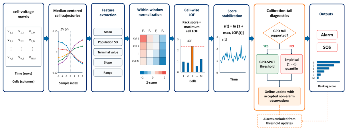
Figure 2.
Stabilized pack score and online threshold for four representative streams. The dashed vertical line marks the calibration boundary and red points indicate alarms. Car18, car10, and LFP high-resistance vin_60 use GPD-SPOT; NCM low-capacity vin_71 uses the empirical fallback after GPD rejection.
Figure 2.
Stabilized pack score and online threshold for four representative streams. The dashed vertical line marks the calibration boundary and red points indicate alarms. Car18, car10, and LFP high-resistance vin_60 use GPD-SPOT; NCM low-capacity vin_71 uses the empirical fallback after GPD rejection.
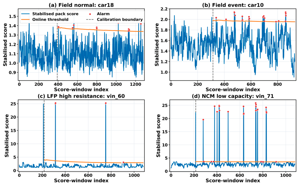
Figure 3.
CH-BatteryGen alarm rates after segment-internal windowing and calibration-tail validation. Hatched bars identify cases using the empirical fallback. Each twenty-segment case has 864 monitoring windows; NCM self-discharge has 692.
Figure 3.
CH-BatteryGen alarm rates after segment-internal windowing and calibration-tail validation. Hatched bars identify cases using the empirical fallback. Each twenty-segment case has 864 monitoring windows; NCM self-discharge has 692.
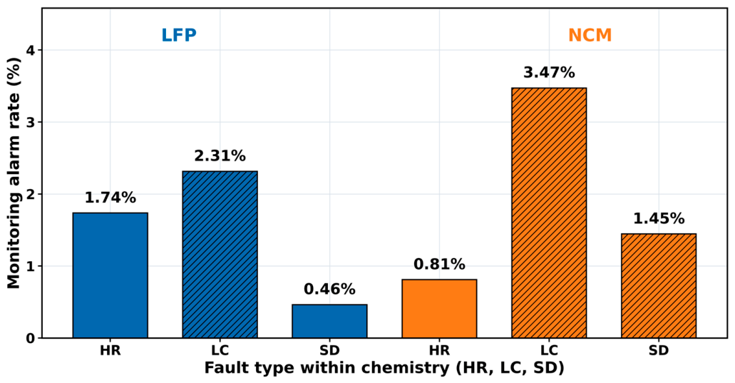
Figure 4.
Normalized mean cell-LOF evidence for the six CH-BatteryGen cases. Red markers show the first-ranked cells. Orange dashed lines indicate the supplied LFP fault-cell labels; no NCM cell labels were supplied.
Figure 4.
Normalized mean cell-LOF evidence for the six CH-BatteryGen cases. Red markers show the first-ranked cells. Orange dashed lines indicate the supplied LFP fault-cell labels; no NCM cell labels were supplied.
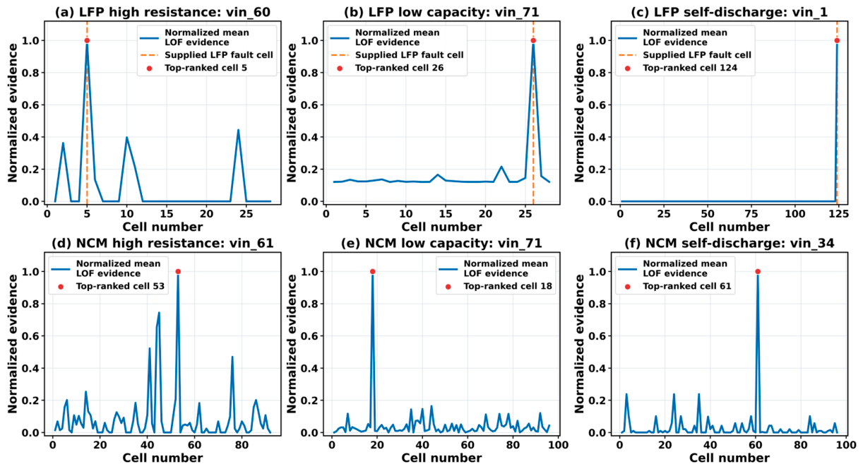
Figure 5.
Operating-condition indicators for the six CH-BatteryGen cases. Values are calculated from the equal-point resampled records and provide context only; they do not enter the warning decision.
Figure 5.
Operating-condition indicators for the six CH-BatteryGen cases. Values are calculated from the equal-point resampled records and provide context only; they do not enter the warning decision.
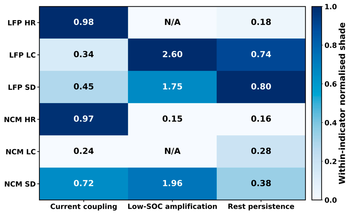
Figure 6.
Sensitivity to tail risk q. (a) panels show the pooled field FAR; (b) event coverage and median lead time; (c) chemistry-mean CH alarm rate; (d) precision/recall under the ±24-h weak-event-window definition.
Figure 6.
Sensitivity to tail risk q. (a) panels show the pooled field FAR; (b) event coverage and median lead time; (c) chemistry-mean CH alarm rate; (d) precision/recall under the ±24-h weak-event-window definition.
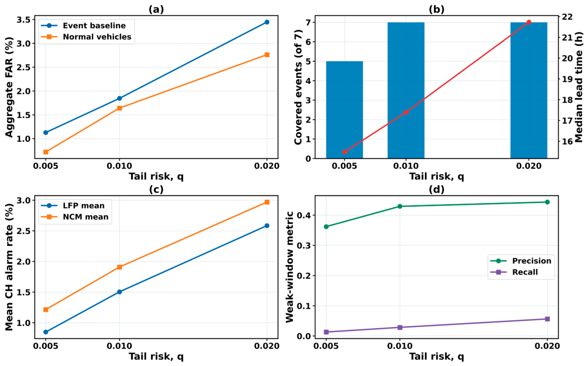
Figure 7.
Direct window-length audit for w = 6, 7 and 8. (a) Case-specific truth-to-runner-up margins; (b) mean margin and top-one result; (c) least-squares slope-variance factor with the corresponding five-minute field span. All windows are segment-internal.
Figure 7.
Direct window-length audit for w = 6, 7 and 8. (a) Case-specific truth-to-runner-up margins; (b) mean margin and top-one result; (c) least-squares slope-variance factor with the corresponding five-minute field span. All windows are segment-internal.
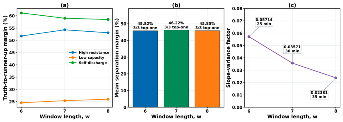
Figure 8.
Empirical calibration survival and fitted unconditional GPD tail for four representative streams. The orange line marks the selected preliminary threshold. The NCM low-capacity tail is shown diagnostically but is rejected and not used online.
Figure 8.
Empirical calibration survival and fitted unconditional GPD tail for four representative streams. The orange line marks the selected preliminary threshold. The NCM low-capacity tail is shown diagnostically but is rejected and not used online.
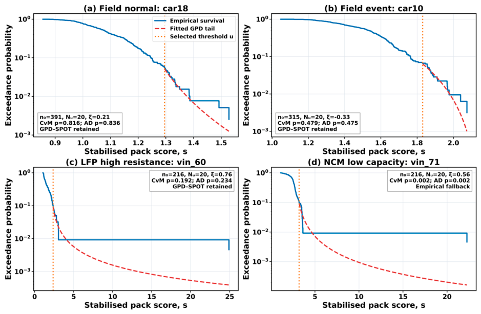
Figure 9.
Mean-excess plots of calibration scores for four representative streams. Blue points show the sample mean excess at each candidate threshold. Orange dashed lines and markers identify the selected preliminary thresholds, each retaining 20 strict calibration excesses.
Figure 9.
Mean-excess plots of calibration scores for four representative streams. Blue points show the sample mean excess at each candidate threshold. Orange dashed lines and markers identify the selected preliminary thresholds, each retaining 20 strict calibration excesses.
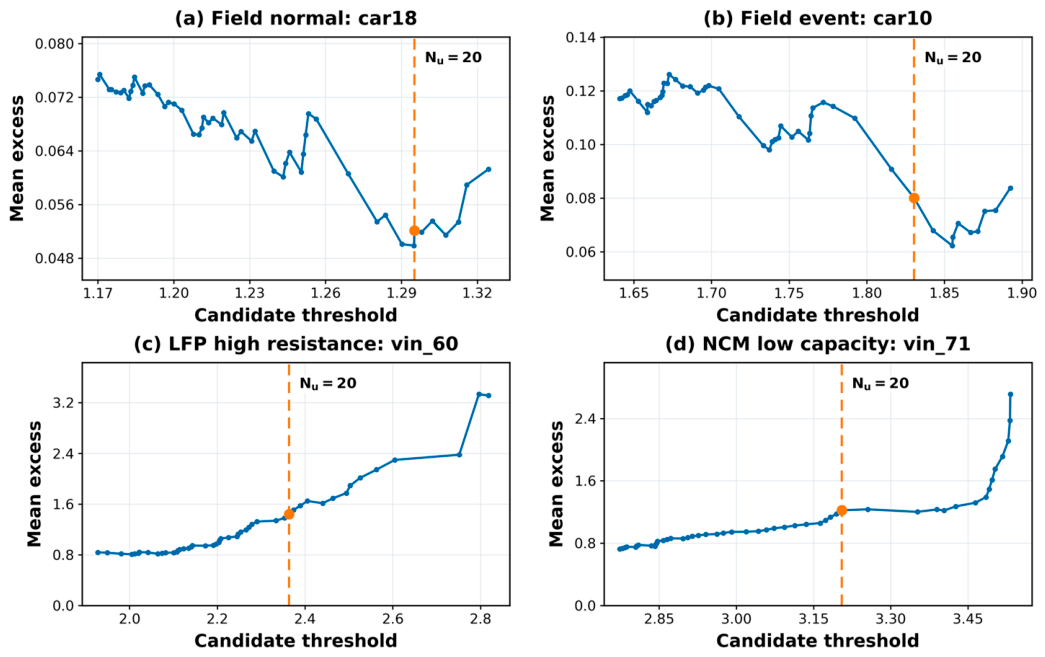
Figure 10.
GPD Q–Q and P–P plots for the selected calibration excesses. Field departures are modest; the NCM low-capacity panels show the upper-quantile and probability distortion that leads to rejection.
Figure 10.
GPD Q–Q and P–P plots for the selected calibration excesses. Field departures are modest; the NCM low-capacity panels show the upper-quantile and probability distortion that leads to rejection.
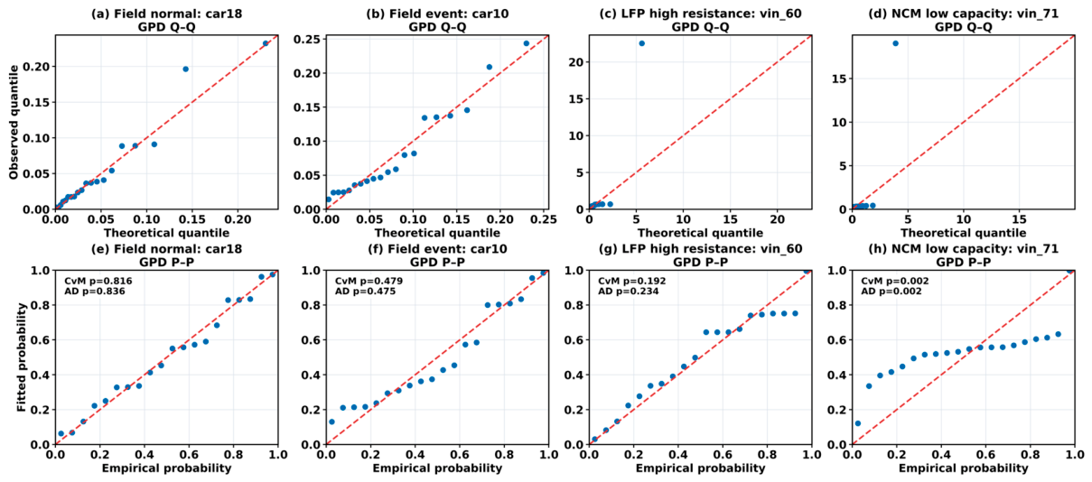
Figure 11.
Alarm-window State-of-Safety results. (a) Field SOS distributions for the event baseline, ±24-h weak event window, and independent normal cohort; (b) CH-BatteryGen case distributions; (c) alarm rate versus median alarm-only SOS. Every non-alarm window has SOS = 100 and is excluded from the boxplots. Lower SOS indicates a larger statistical score-threshold gap, not lower measured electrochemical safety. Points from overlapping windows are descriptive and are not treated as independent replicates.
Figure 11.
Alarm-window State-of-Safety results. (a) Field SOS distributions for the event baseline, ±24-h weak event window, and independent normal cohort; (b) CH-BatteryGen case distributions; (c) alarm rate versus median alarm-only SOS. Every non-alarm window has SOS = 100 and is excluded from the boxplots. Lower SOS indicates a larger statistical score-threshold gap, not lower measured electrochemical safety. Points from overlapping windows are descriptive and are not treated as independent replicates.
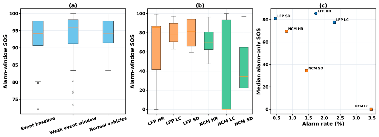
Figure 12.
Retrospective audit of pre-event voltage morphology. Each blue marker is a ten-minute median of the selected candidate cell’s pack-relative low-side residual during the 24 h before the source timestamp; blue lines are broken when successive observations are more than 30 min apart, and the red dashed line marks the source event. Candidate cells were selected from the final-two-hour 95th-percentile residual independently of LOF and SPOT. Coverage and maximum gap quantify temporal continuity. Vertical scales differ among panels.
Figure 12.
Retrospective audit of pre-event voltage morphology. Each blue marker is a ten-minute median of the selected candidate cell’s pack-relative low-side residual during the 24 h before the source timestamp; blue lines are broken when successive observations are more than 30 min apart, and the red dashed line marks the source event. Candidate cells were selected from the final-two-hour 95th-percentile residual independently of LOF and SPOT. Coverage and maximum gap quantify temporal continuity. Vertical scales differ among panels.
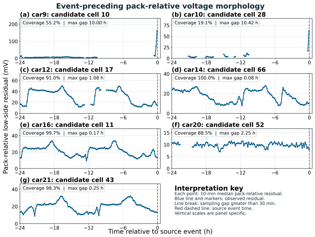

Table 1.
Data composition and analytical role.
| Source | Composition | Available variables | Processing interval | Analytical role |
|---|---|---|---|---|
| Field event cohort |
7 independent vehicles (car9, car10, car12, car14, car16, car20, and car21.) |
Cell voltage; current; SOC; alarm/event time | 7-day before to 1-day after source event; 5-min resampling | False-alarm rate, events with a pre-event alarm, lead time, and event-label metrics |
| Field normal cohort | 2 independent vehicles (car18, car19) | Cell voltage; current; SOC | 8-day interval ending on 31st Oct 2022; 5-min resampling |
Independent normal false-alarm reference |
| CH-BatteryGen LFP | 3 selected cases; 20 segments each | Numerical VOLT channels; current; SOC; three cell labels | 60 equal-index rows per segment; segment-internal windows; first 20% calibration | Fault-dependent observability, cell localization, context |
| CH-BatteryGen NCM | 3 selected cases; 20, 20, and 16 segments | Numerical VOLT channels; current; SOC; no uploaded cell labels | 60 equal-index rows per segment; segment-internal windows; first 20% calibration | Chemistry–fault comparison and candidate-cell ranking |
Table 2.
Provenance of derived variables.
| Quantity | Source and derivation | Reported form | Use |
|---|---|---|---|
| Field event time | Earliest bit-64 voltage alarm for car9/car10; fault-time CSV for car12/car14/car16/car20/car21 |
No manual time shift | Lead time and ±24-h event-label interval |
| Field voltage matrix | Modal-length voltage lists after sorting, duplicate-time removal, and 5-min last-value resampling | Time × cell matrix | LOF feature input |
| CH voltage matrix | Cycle-paired segments; 60 equal-index rows per segment; seven-point windows formed within each segment only | Time × cell matrix | LOF feature input |
| CH P95 spread | For segment s, select rs,j = floor[j(ns−1)/59], j=0,…,59; then pool ΔVs,j = 1000(maxiVi−miniVi) and take the linearly interpolated 95th percentile | mV; equal segment weight | Upper-tail voltage-dispersion descriptor; not an alarm input |
| Cell evidence | Mean cell LOF over alarm windows; all monitoring windows only if no alarm | Normalized to case maximum for Figure 4 | Suspicious-cell ranking |
| Context indicators | Resampled CH voltage spread combined with current and SOC | Correlation or dimensionless ratio | Visibility context; not mechanism proof |
Table 3.
Fixed method parameters and tested alternatives.
| Parameter | Main setting | Reason | Sensitivity setting |
|---|---|---|---|
| Window length w | 7 samples | 3/3 LFP top-one; largest direct w=6–8 mean separation margin (46.22%); 30-min field span | Direct: 6 and 8; broad sweep: 5 and 9 samples |
| Feature normalization | z-score across cells within each window | Equal scale; no future windows; zero-variance feature set to zero | Fixed |
| LOF neighbours k | 20, capped at M−1 | Fixed cell-wise locality setting; exact-tie limitation reported | k = 15 and 25 |
| Pack aggregation | Maximum cell LOF | Retains single-cell abnormality | Fixed |
| Score | ln(1 + maximum LOF) | Monotonic stabilisation of large density ratios | Fixed |
| SPOT preliminary tail | pᵤ = min [0.98, max(0.80, 1 − 20/n0)] | 20 strict calibration excesses in every stream | Tail plots and bootstrap tests |
| SPOT risk q | 0.01 | Smallest tested q with a pre-event alarm for all 7 events | 0.005 and 0.020 |
| Field calibration | First 48 h | Initial source-timestamped period; fixed before outcome comparison | Not re-optimised |
| CH calibration | First 20% | Index-based calibration; fixed before outcome comparison | Not re-optimised |
| Tail-model gate | Use GPD only if CvM and AD p≥0.05 and ξ<1; otherwise empirical quantile | Validity gate prevents rejected extrapolation | 500 bootstrap replicates |
| SOS scaling | α = 1 | Direct exponential mapping of stabilised exceedance | Fixed |
Table 4.
Vehicle-level field warning results.
| Vehicle | Source event time | Monitoring windows | Baseline windows | Baseline alarms | Baseline FAR (%) | Event-window alarms/ monitored windows |
Pre-event lead (h) |
|---|---|---|---|---|---|---|---|
| car9 | 2020-01-14 08:56:00 | 778 | 573 | 6 | 1.05 | 3/205 | 22.43 |
| car10 | 2020-01-14 08:18:12 | 615 | 419 | 15 | 3.58 | 6/196 | 0.053 |
| car12 | 2022-09-09 14:04:58 | 1617 | 1083 | 21 | 1.94 | 8/534 | 10.83 |
| car14 | 2022-08-05 05:06:17 | 1657 | 1083 | 19 | 1.75 | 24/574 | 19.85 |
| car16 | 2022-07-27 17:13:38 | 1721 | 1146 | 7 | 0.61 | 5/575 | 17.39 |
| car20 | 2022-06-02 21:01:02 | 1645 | 1107 | 29 | 2.62 | 23/538 | 15.43 |
| car21 | 2022-10-29 14:54:08 | 1715 | 1146 | 24 | 2.09 | 22/569 | 21.74 |
| car18 | Normal interval | 889 | 889 | 12 | 1.35 | — | — |
| car19 | Normal interval | 1609 | 1609 | 29 | 1.80 | — | — |
Table 5.
Aggregate field results and denominator definitions.
| Population/period | Alarms | Windows | Rate (%) | Event-level result | Interpretation |
|---|---|---|---|---|---|
| Event-labelled pre-event baseline | 121 | 6557 | 1.845 | 7/7 events had a pre-event alarm | Median lead 17.39 h; one case 0.053 h |
| Independent normal vehicles | 41 | 2498 | 1.641 | No event label | car18 1.35%; car19 1.80% |
| ±24-h event-label intervals | 91 | 3191 | 2.852 | Precision 0.429 | Recall 0.029 |
Table 6.
CH-BatteryGen case-level alarm, SOS, and resampled voltage-spread results.
| Chemistry | Fault | Case | Segments | Monitoring windows | Alarms | Alarm rate (%) | All-window mean SOS | Minimum SOS | Resampled P95 spread (mV) |
|---|---|---|---|---|---|---|---|---|---|
| LFP | high resistance | vin_60 | 20 | 864 | 15 | 1.74 | 99.37 | <0.01 | 132.15 |
| LFP | low capacity | vin_71 | 20 | 864 | 20 | 2.31 | 99.53 | 62.70 | 26.05 |
| LFP | self-discharge | vin_1 | 20 | 864 | 4 | 0.46 | 99.90 | 59.68 | 12.00 |
| NCM | high resistance | vin_61 | 20 | 864 | 7 | 0.81 | 99.77 | 47.34 | 78.00 |
| NCM | low capacity | vin_71 | 20 | 864 | 30 | 3.47 | 97.54 | <0.01 | 97.00 |
| NCM | self-discharge | vin_34 | 16 | 692 | 10 | 1.45 | 99.22 | 19.20 | 45.00 |
SOS values below 0.01 are printed as <0.01 due to exponential numerical saturation; they do not represent zero physical safety.
Table 7.
Suspicious-cell localization and operating-condition indicators.
| Chemistry | Fault | Case | Supplied fault cell | Top-ranked cell by LOF | Supplied-cell rank | Current coupling | Low-SOC amplification | Rest persistence |
|---|---|---|---|---|---|---|---|---|
| LFP | high resistance | vin_60 | 5 | 5 | 1 | 0.98 | — | 0.18 |
| LFP | low capacity | vin_71 | 26 | 26 | 1 | 0.34 | 2.60 | 0.74 |
| LFP | self discharge | vin_1 | 124 | 124 | 1 | 0.45 | 1.75 | 0.80 |
| NCM | high resistance | vin_61 | Not supplied | 53 | Not assessed | 0.97 | 0.15 | 0.16 |
| NCM | low capacity | vin_71 | Not supplied | 18 | Not assessed | 0.24 | — | 0.28 |
| NCM | self discharge | vin_34 | Not supplied | 61 | Not assessed | 0.72 | 1.96 | 0.38 |
Table 8.
Main parameter-sensitivity results.
| q | Event baseline FAR (%) | Normal FAR (%) | Events with pre-event alarm | Median lead (h) | Precision | Recall | Mean LFP alarm rate (%) | Mean NCM alarm rate (%) |
|---|---|---|---|---|---|---|---|---|
| 0.005 | 1.129 | 0.721 | 5/7 | 15.49 | 0.362 | 0.013 | 0.849 | 1.215 |
| 0.010 | 1.845 | 1.641 | 7/7 | 17.39 | 0.429 | 0.029 | 1.505 | 1.909 |
| 0.020 | 3.447 | 2.762 | 7/7 | 21.74 | 0.443 | 0.056 | 2.585 | 2.970 |
Window-length selection note: in a segment-internal audit, w = 6, 7 and 8 all retained the three supplied LFP cells at rank one; Mean labelled-cell separation margin across the three LFP cases were 45.82%, 46.22%, and 45.85%, respectively; The w = 7 setting was retained as the central variance–latency operating point.
Table 9.
Alarm-window SOS magnitude reported separately from alarm frequency.
| Population or case | Threshold method | Alarms | Windows | Rate (%) | Median alarm SOS | Alarm SOS IQR | Minimum SOS | SOS < 75, n (%) |
|---|---|---|---|---|---|---|---|---|
| Event baseline | GPD-SPOT | 121 | 6557 | 1.845 | 93.98 | 90.33–97.62 | 72.08 | 1 (0.8) |
| ±24-h event window | GPD-SPOT | 91 | 3191 | 2.852 | 95.96 | 91.15–98.22 | 73.48 | 1 (1.1) |
| Independent normal | GPD-SPOT | 41 | 2498 | 1.641 | 94.19 | 91.48–97.77 | 83.37 | 0 (0.0) |
| LFP HR | GPD-SPOT | 15 | 864 | 1.736 | 85.38 | 41.39–86.88 | <0.01 | 4 (26.7) |
| LFP LC | Empirical fallback | 20 | 864 | 2.315 | 77.71 | 70.57–89.93 | 62.70 | 9 (45.0) |
| LFP SD | GPD-SPOT | 4 | 864 | 0.463 | 81.04 | 65.87–94.14 | 59.68 | 2 (50.0) |
| NCM HR | GPD-SPOT | 7 | 864 | 0.810 | 69.57 | 62.24–80.80 | 47.34 | 4 (57.1) |
| NCM LC | Empirical fallback | 30 | 864 | 3.472 | <0.01 | <0.01–93.48 | <0.01 | 21 (70.0) |
| NCM SD | Empirical fallback | 10 | 692 | 1.445 | 34.42 | 22.52–64.79 | 19.20 | 8 (80.0) |
Only alarm windows are summarised in the median, IQR, minimum, and SOS < 75 column; every non-alarm window equals 100. Lower SOS denotes a larger statistical score-threshold gap, not lower measured electrochemical safety. Overlapping windows are descriptive observations, not independent replicates.
Table 10.
Retrospective audit of pre-event voltage morphology.
| Vehicle | Candidate cell | Direction | Coverage (%) | Maximum gap (h) | Early median (mV) | Final 2 h median (mV) | b (mV h−1) | p | Supported interpretation |
|---|---|---|---|---|---|---|---|---|---|
| car9 | 10 | Low-side | 55.2 | 10.00 | 5.00 | 18.00 | 0.057 | 0.302 | Indeterminate: late separation; onset falls across a 10.00-h gap |
| car10 | 28 | Low-side | 19.1 | 10.42 | 3.00 | 34.00 | 0.378 | <0.001 | Indeterminate: positive trend, but a 10.42-h gap spans the rise |
| car12 | 17 | Low-side | 91.0 | 1.08 | 39.00 | 15.50 | -0.816 | <0.001 | No progressive rise; residual decreases |
| car14 | 66 | Low-side | 100.0 | 0.08 | 18.75 | 10.00 | -0.344 | <0.001 | No progressive rise; residual decreases |
| car16 | 11 | Low-side | 99.7 | 0.17 | 23.50 | 16.00 | -0.282 | <0.001 | No progressive rise; residual decreases |
| car20 | 52 | Low-side | 88.5 | 2.25 | 10.00 | 9.75 | 0.000 | 0.124 | Stable within the pre-event window |
| car21 | 43 | Low-side | 98.3 | 0.25 | 20.00 | 15.00 | 0.071 | 0.190 | Non-monotonic; no sustained rise |
Residuals are candidate-cell deviations from the pack median; positive values denote that the candidate is below the median. Coverage is the percentage of the 288 expected five-minute bins observed during the 24 h before the source event. Maximum gap is calculated between successive valid five-minute records. Early and final-two-hour medians also use the five-minute residuals. The Theil-Sen slope b and Mann-Kendall p-value use ten-minute median residuals in bins anchored at T−24 h. Indeterminate cases do not meet the evidential criteria for either progressive-like or abrupt-like morphology. The table describes observed voltage morphology and does not assign a physical fault mechanism.
Disclaimer/Publisher’s Note: The statements, opinions and data contained in all publications are solely those of the individual author(s) and contributor(s) and not of MDPI and/or the editor(s). MDPI and/or the editor(s) disclaim responsibility for any injury to people or property resulting from any ideas, methods, instructions or products referred to in the content. |
© 2026 by the authors. Licensee MDPI, Basel, Switzerland. This article is an open access article distributed under the terms and conditions of the Creative Commons Attribution (CC BY) license (http://creativecommons.org/licenses/by/4.0/).
Copyright: This open access article is published under a Creative Commons CC BY 4.0 license, which permit the free download, distribution, and reuse, provided that the author and preprint are cited in any reuse.