

Submitted:
12 September 2026
Posted:
15 September 2026
You are already at the latest version
Abstract
A moving optical tweezer builds a defect-free atom array one move at a time, and the same tweezer would refill the array during sustained error correction. Both tasks are the same process: a count of vacancies served by passes whose duration grows with the number of atoms moved, while the array loses atoms at a rate set by its lifetime and its imaging. We write that process as a map on the vacancy count, calibrate it to the published cryogenic 2,000-site experiments (a 5,000 s lifetime, 0.15% loss per image, about a millisecond per move, 1.3% transport loss, a 1.3 s cycle overhead), and check it against a discrete-event simulation with conservation-law invariants. Read as shot-based assembly, the map reproduces the second cycle of the published 1,024-atom result: from the 135 vacancies the experiment reports entering that cycle, one pass leaves 3.2 to 4.2 against 3.1 measured, and at the map's residual floor of 1.8 holes the defect-free fraction is 10 to 16 percent against ``more than ten''. (The first cycle relocates nearly every loaded atom and is a compaction, not a pass over vacancies; it is outside the map.) The residual is \(N(p c_0 + p_d)/(1 - p_t)\), dominated by the per-image loss \(p_d\), so the largest array assembled defect-free with order-one probability is about 560 atoms at the measured imaging loss, 1,300 at 0.05% and 2,700 at 0.01%, and adding moving beams changes none of these numbers. Read as a sustained reload loop at a 100 ms detection-to-repair latency, the map says the opposite: at low move duty the standing vacancy density is \(p c_0\) whatever the tweezer does, and the array size one moving beam can serve is set by its parallelism: \(1.3 \times 10^4\) sites for the linear pass a moving tweezer is expected to have at the vacancy counts of a loop, falling to 1,200 if the pass duration grows as \(n^{1.5}\), and scaling as \(m^{1/\gamma}\) with \(m\) beams. The exponent \(\gamma\) is a property of the move planner, and the two measurements that fix the roadmap are the pass duration against the number of moves with the planner held fixed, and the per-image loss.
Keywords:
neutral-atom arrays
; optical tweezers
; atom rearrangement
; defect-free assembly
; atom loss
; sustained error correction
; erasure
; resource estimation
; discrete-event simulation
1. Introduction
Rubidium tweezer arrays at cryogenic temperature now hold single atoms for thousands of seconds [1] and are assembled defect-free at the thousand-atom scale by a single moving tweezer that transports one atom per move [2,3]. The same architecture is a candidate for the sustained operation that error correction requires, where a lost atom is carried by the code as a located erasure until a rearrangement pass refills its site [4,5,6], and where continuous refilling has been demonstrated on other platforms with deflector-pair rearrangement [7,8] and lattice reloading [9].
Assembly and refilling are usually treated as different problems with different figures of merit: assembly as a budget of trap lifetime against assembly time, refilling as a rate of loss against a rate of reload. They are the same process. In both, a count of vacancies is served by passes whose duration depends on how many atoms they move, while the array keeps losing atoms during the pass. The companion paper [10] writes this process as a queue with state-dependent service and studies it for the deflector-pair architecture; here we specialize it to the moving tweezer, where the per-atom cost is a fixed millisecond and the pass duration is set by the planner, and we calibrate every coefficient to the cryogenic experiments.
The two readings of the map give opposite design levers. In assembly the residual vacancy count is set by the losses during one cycle, which at cryogenic lifetimes are the per-image detection loss and almost nothing else; the number of moving beams does not enter, and the defect-free size limit is a statement about imaging. In a sustained loop the standing vacancy density is set by the detection-to-repair latency, again independent of the tweezer; but the array size the loop can serve at all is set by the tweezer’s throughput, that is, by its parallelism, and by how the pass duration grows with the number of moves. Section 2 states the map and its calibration, Sec. Section 3 checks it against the published assembly, Sec. Section 4 derives the assembly size limit, Sec. Section 5 gives the loop’s size limit and its scaling with parallelism, and Sec. Section 7 names the two measurements that fix both.
2. One Map Serves Assembly and Reload
2.1. Assembly and Reload Differ Only in Whether the Reservoir Refills
An array has N target sites and D vacancies. Time is measured in units of 10 ms, the syndrome round of a sustained loop, and we call that unit a round even in the assembly reading. Each round every atom present is lost with probability p, so the array loses a Poisson number with mean . A pass images the array (a per-atom loss ), plans, and moves n atoms from a reservoir into the vacant sites, lasting
with the fixed overhead of imaging, planning and transfer, the per-move cost and the exponent with which the pass grows in its content. A moved atom arrives with probability ; the site of a lost atom stays vacant. The greedy pass takes every vacancy present, and at pass boundaries, with losses at their mean, the vacancy count obeys
The first term is the vacancies the pass failed to fill; the second is the loss during the pass, in flight and at the image.
Assembly is the map iterated from the stochastic load: for a fill fraction f, a reservoir equal to the surplus of the load that is not refilled, and after k cycles; for Poisson holes the defect-free probability is . The sustained loop is the same map with a reservoir that is refilled and a pass that starts whenever a vacancy is present; its working point is the stable fixed point of Eq. (2), and for the map can also have an unstable fixed point above which each pass takes longer than the losses it repairs [10]. Nothing in the map distinguishes the two readings except whether the reservoir refills.
2.2. Every Coefficient Comes from the Cryogenic Experiments
The moving-tweezer coefficients come from the two published assemblies in 2,000-site cryogenic arrays. The 4 K experiment [3] assembled 1,024 atoms in a 2,070-trap two-wavelength array and reports a vacuum lifetime of about 5,000 s, a detection loss of per image, transport survival of and move success of , a first cycle of about 2 s with about 1,014 moves and a second of about 1.5 s with 135 moves, an average defect rate of , and defect-free registers in more than ten percent of realizations. Its predecessor at 6 K [2] assembled 828 atoms in 2,088 sites, from a load, in cycles of about 1.65 s (about 150 ms of planning, 500 ms of transfer, and under a second of execution for about 800 moves), with a lifetime of about 100 s at the time, and reached occupancy after two cycles. Trap lifetimes of 6,000 s have been measured in the same kind of cryostat [1].
From these: the per-move cost is about a millisecond, round, and it does not depend on N; the cycle overhead is what remains of a cycle once its moves are subtracted at a millisecond each, about 1.3 s from the second cycle (1.5 s less 135 ms) and about 1 s from the first (2 s less 1,014 ms), and we take rounds for assembly; the background loss is per round at 5,000 s; the per-image loss is , which we read as the loss per image (if the published figure is a survival per rearrangement sequence rather than per image, the per-image loss is smaller and the assembly limit of Sec. Section 4 is pessimistic by the same factor); the transport loss is from the transport survival alone and with the failed moves stacked on, and we carry both. Stacking the failed moves onto the loss is conservative, since a failed move usually leaves the atom in its origin trap, where it is still in the reservoir for the next cycle. For the sustained loop of Sec. Section 5 the overhead is the detection-to-repair latency rather than today’s planning and transfer time, and we take rounds (100 ms), the value of the companion paper, so that the two architectures share a cadence; the loss rate there is operational, readout loss on the atoms imaged and Rydberg loss on the atoms gated, and at the measured per image with half the atoms imaged every round it is , which we round to the bracket , with as the gate-loss bracket. The 10 ms round, the half-array mid-circuit imaging and the 100 ms latency are design targets like itself, not measurements; the bracket is an atom that survives ten rounds and is a bound rather than a scenario. The exponent is the one number no experiment reports, and Sec. Section 6 says why it is a property of the planner.
2.3. A Discrete-Event Run Checks the Map Under Conservation Laws
The map is deterministic and at pass boundaries. The stochastic process behind it was run as a discrete-event world on the verification-first engine of the companion paper [10]: one state machine whose every transition publishes a projection checked against nine runtime invariants, two of which are conservation laws (every vacancy was made by a loss and unmade only by a repair; every atom taken from the reservoir either filled a site or was lost in transit). Randomness enters through two uniforms per round and one per pass, converted to counts by inverse CDF, so paired arms consume the same draws and an audit confirms it. The per-image loss is folded into the per-round rate as in the engine and kept separate in the map. Error bars are 95% half-widths; every run reported here completed with no invariant finding.
3. The Map Reproduces the Published 1,024-Atom Assembly
The first cycle of a shot-based assembly is not a pass over vacancies. The loaded atoms sit at random positions in a 2,000-site array, and the first cycle relocates nearly all of them into the target region: about 1,014 moves for the 1,024-site target and about 800 for the 828-site one, of order N rather than of order the vacancy count, with a reservoir that is the margin of the load over the target (a load of 2,070 traps is about 1,035 atoms for 1,024 sites). That compaction is outside the map, whose pass moves one atom per vacancy, and it is why the experiment entered its second cycle with 135 vacancies where a vacancy pass from a half-filled target would leave about ten. The map describes the second cycle and every cycle after it, which is the regime a sustained loop lives in, and that is the check made here. Table 1 runs the assembly reading at the calibration of Sec. Section 2.2 from the measured start of the experiment’s second cycle (, one pass), then iterates the map’s own passes from a half-filled target (, two passes) to reach its residual floor, with the room-temperature-lifetime predecessor beside it.
From 135 holes, one pass leaves 3.2 to 4.2 against the measured average of 3.1. The map’s own passes converge to 1.9 to 2.0 holes, the floor of Sec. Section 4, where the engine’s defect-free fraction is 10 to 11 percent against the published “more than ten”. The engine and the map agree to three percent in every cell, which is the statement that shot-based assembly is the vacancy map with the reservoir not refilled. The 828-atom assembly is reproduced to within the uncertainty of its lifetime: the map puts the residual at at the reported 100 s and at at 40 s against measured, and the lifetime during that run is the least certain of the inputs. Two differences are informative. The map’s Poisson defect-free fraction from the floor of Sec. Section 4 is where the engine measures 10 to 11 percent; the engine’s holes after the second pass have a variance above the mean because the transport failures of the first pass propagate, and the published fraction sits between the two. And the direct comparison from 135 holes gives a defect-free fraction of 1 to 3 percent, below the published ten, at the same mean: the published hole distribution is narrower than Poisson, which a scalar model cannot represent and which the experiment’s per-shot hole counts would settle.
4. Detection Loss Sets the Assembly Size Limit
The fixed point of Eq. (2) in the assembly reading is the residual the cycles converge to,
since is negligible against once D is small. At the cryogenic calibration the two terms in the numerator are and : the per-image loss is six times the background loss over the whole 1.3 s cycle, and the residual of 1.8 holes at is 1.5 of them from the image. Three consequences follow.
The largest array that can be assembled defect-free with order-one probability is where the floor reaches one hole,
which is 560 atoms at the measured and , 1,300 at , and 2,700 at ; at with the overhead cut to 100 ms it is 8,000 (Table 2, Figure 1). The defect-free probability at a given N is for Poisson holes, so the 1,024-atom experiment sits at and a 2,048-atom target at the same imaging loss would be defect-free in about two percent of shots.
Parallelism does not enter. With m moving beams the per-move cost is , the cycle is shorter by at most the execution time, and the residual after two cycles from a half-filled 1,024-site target is 2.0 holes for and 8 alike; at 2,048 sites it is 4.0 for every m. Faster moves shorten the cycle that the reservoir atoms wait through, which at a 5,000 s lifetime costs nothing, and do not touch the image. The lever for assembly is first and second, and Table 2 says by how much: at the measured imaging loss, cutting the overhead from 1.3 s to 100 ms buys 15 percent in ; at imaging loss it buys a factor of three.
The room-temperature ceiling is the same formula with the background term restored. At a 20 s lifetime, a 100 ms cycle and imaging loss, is about a hundred atoms; at 60 s and it is about three hundred. That is why room-temperature assembly saturated at a few hundred atoms and why the cryogenic lifetime, which removes the first term, was what allowed the thousand-atom milestone; and it is why the next factor of two is in the second term, which the cryostat does not touch.
5. Parallelism Sets the Reload-Loop Size Limit
In the sustained reading the reservoir refills and a pass starts whenever a vacancy is present. Two things then hold at every array size, and a third depends on the size.
At low move duty the standing vacancy density is , whatever the tweezer does. A vacancy detected at one image stands until the pass that follows the next one, so the working point is about vacancies plus the content of the pass in flight: at and , one percent of the array, the same density a deflector pair leaves at the same cadence. The pass in flight grows with the move duty (Table 3: 1.1 percent of the array at a thousand sites, 4.4 percent at eight thousand), so the floor is the latency’s alone only while the beam is mostly idle. The remedy for that floor is a shorter detection-to-repair latency, not a faster tweezer.
The pass cannot be served one atom at a time: with a one-move pass costs ten rounds, so the loop batches, and the batch it can sustain is bounded by its throughput. At the loop keeps up while the move duty is below , that is below sites at and 980 at , and the working point climbs toward that line.
The array size one beam can serve depends on the exponent (Table 3), and Sec. Section 6 says why is the expectation for a moving tweezer at these vacancy counts and the risk case. At the working point is 11 vacancies at a thousand sites, 67 at four thousand and 355 at eight thousand, with the measured mean about 1.5 times the map’s value at every size (the pass in flight), no crossing in any replication, and the working point passing a quarter of the array near sites. At the loop has a basin at a thousand sites, a working point of 17 with an unstable boundary at 96, and a burst of 64 vacancies is recovered in every replication; at two thousand sites the working point is gone and every replication diverges from zero with no burst at all. At the working point is gone between two and three thousand sites; at , near five hundred. At the gate-loss bracket the limits are 900, 310 and below 250 sites for , and .
Parallelism is the lever here, and its return diminishes with the exponent (Table 4, Figure 2). With m beams the per-move cost is ; for the unstable boundary is , and the size at which it meets the working point scales as : linearly for a linear pass, as at , as for a quadratic one. Sixteen beams carry a linear pass to sites and a pass to 7,400. A hybrid that uses a deflector pair for the bulk and the moving tweezer for the residue is, in the map, a large m for the scattered vacancies and a small one for the clustered ones, and which of the two governs is the exponent question of the next section.
6. The Exponent Is a Property of the Planner
For a deflector pair the pass duration is concave in the number of vacancies, because one step moves a whole row and the number of distinct rows hit saturates [10]. For a moving tweezer every move is one step, so the execution time is linear in the number of moves by construction, and the only place an exponent above one can enter is the planning: the assignment of reservoir atoms to vacancies is solved exactly (cubic in the count) or greedily (linear), and the ordering of the moves so that no move crosses an occupied site ranges from linear to quadratic in the number of moves depending on the algorithm. The published cycles planned about 800 to 1,000 moves in about 150 ms. A planner with that cost at a thousand moves, even if cubic, costs milliseconds or less at the tens to low hundreds of moves a sustained loop presents, well below the 100 ms latency ; so at loop vacancy counts the expectation for a moving tweezer is , a pass dominated by its fixed overhead, and the size limit is the linear row of Table 4. The rows are the risk case: a pass that is replanned with a collision-avoidance step whose cost grows with the occupied density rather than with the move count, or a pass that waits on a reservoir refill that itself scales with the vacancy count. A planner quadratic in the count would give the loop of Table 3 at to 2, with a basin of a few hundred atoms and a size limit of a thousand, where the linear case gives . The exponent is therefore a software choice, and the map says which choice to make: the linear heuristic, replanned per pass, even at some cost in move count. The measurement that establishes the exponent is the pass duration against the number of moves, at operating density, with the planner held fixed and named in the report.
7. Two Measurements Fix the Roadmap
The assembly limit of Sec. Section 4 and the loop limit of Sec. Section 5 each rest on one number the experiments can measure directly.
The first is the per-image loss , separately from the background loss. The published is the sum of the two over a cycle; at a 5,000 s lifetime the background part is and the rest is the image, and Eq. (4) says that each factor of three in is a factor of two to three in the defect-free size. The per-shot hole distribution, not only its mean, is the second half of this measurement, since the published defect-free fraction above ten percent at a mean of 3.1 holes says the distribution is narrower than Poisson, and the model’s is then a lower bound.
The second is the pass duration against the number of moves, with the planner fixed, over the range of vacancy counts a sustained loop would present (tens to hundreds), at two array sizes. It gives and together, and with p and it places the machine in Table 4: the number of moving beams the roadmap needs at each array size follows from the row.
8. Scope and Limitations
The model is a scalar vacancy count with a single per-round loss rate. It carries no geometry, so it cannot say where the residual holes of an assembly are or how a hole distribution narrower than Poisson arises; the sustained reading draws one loss rate for imaged and gated atoms alike where a real loop loses atoms per operation, and the companion paper’s distance-tax estimate, which depends on where the holes stand, is not repeated here for that reason. The assembly calibration reads its inputs from the published text of two experiments and is a check of the map’s form, not a fit: the cycle overhead is inferred from the difference of two cycle times, the per-image loss is folded into the engine’s per-round rate, and the 828-atom lifetime during its run is uncertain by a factor of two. The sustained loop’s rounds is a design target, not a measured value; today’s shot-based overhead is 130 rounds, and the standing density scales with whichever is achieved. The reservoir’s refill rate in the loop studies ( per round) is an assumption with no measurement behind it, and a reservoir loaded from a magneto-optical trap or a conveyor is itself imaged and lost like the array. The exponent is the declared unknown, and the parallelism table is a statement about the map, checked stochastically at one beam only. A reservoir that is itself refilled in batches, once per magneto-optical-trap cycle, would show the working point as a sawtooth at that period.
Use of AI Assistance
This paper was produced with an AI assistant (Claude, Anthropic; the Claude Fable 5.1 model as configured in the working sessions) used as a research and writing collaborator under the author’s direction. The assistant wrote the simulation world on the author’s verification-first engine, ran the studies, computed the tables from the map, drafted the manuscript and produced the figures; the author posed the question, chose the calibration, directed each revision and checked the results, and is responsible for the content. All published values in Sec. 2.2 were taken from the cited sources.
Reproducibility and data availability
Every number traces to the worlds/atomarray world in the polysim repository: run-sequential.mjs produces the file sequential-results.json behind Table 1 and Table 3; theory.mjs holds the map, the assembly iteration and the size-limit bisection (Table 2 and Table 4, written to figs/parallelism.json); the machine, its contract and its nine invariants are in machines/reloadzone/; atomarray.test.mjs pins the assembly residual and the size limits at reduced size; the figures are rendered by figs/make_figs_mt.py. The model is fully specified by Eqs. (1) and (2) and can be reimplemented in any discrete-event framework.
References
- Schymik, K.-N.; Pancaldi, S.; Nogrette, F.; Barredo, D.; Paris, J.; Browaeys, A.; Lahaye, T. Single atoms with 6000-second trapping lifetimes in optical-tweezer arrays at cryogenic temperatures . Phys. Rev. Appl. 2021, 16, 034013. [Google Scholar] [CrossRef]
- Pichard, G.; Lim, D.; Bloch, E.; Vaneecloo, J.; Bourachot, L.; Both, G.-J.; Mériaux, G.; Dutartre, S.; Hostein, R.; Paris, J.; Ximenez, B.; Signoles, A.; Browaeys, A.; Lahaye, T.; Dreon, D. Rearrangement of individual atoms in a 2000-site optical-tweezer array at cryogenic temperatures . Phys. Rev. Appl. 2024, 22, 024073. [Google Scholar] [CrossRef]
- Lim, D.; Mamann, H.; Pichard, G.; Bourachot, L.; Lindberg, A.; Hamot, C.; Le Bars, H.; Fasola, F.; Tan, S.; Cournez, G.; Dutartre, S.; Cartry, T.; Lemettre, S.; Hostein, R.; Paris, J.; Ferreyrol, F.; Collardey, A.; Signoles, A.; Lahaye, T.; Monmeyran, C.; Ximenez, B. Defect-free arrays at the thousand-atom scale in a 4-K cryogenic environment . PRX Quantum 2026, 7, 033032. [Google Scholar] [CrossRef]
- Wu, Y.; Kolkowitz, S.; Puri, S.; Thompson, J. D. Erasure conversion for fault-tolerant quantum computing in alkaline earth Rydberg atom arrays . Nat. Commun. 2022, 13, 4657. [Google Scholar] [CrossRef]
- Ma, S.; et al. High-fidelity gates and mid-circuit erasure conversion in an atomic qubit . Nature 2023, 622, 279. [Google Scholar] [CrossRef]
- Scholl, P.; et al. Erasure conversion in a high-fidelity Rydberg quantum simulator . Nature 2023, 622, 273. [Google Scholar] [CrossRef]
- Chiu, N.-C.; et al. Continuous operation of a coherent 3,000-qubit system . Nature 2025, arXiv:2506.20660646, 1075. [Google Scholar] [CrossRef]
- Atom Computing and Collaborators. Quantum Error Correct. With Toric Code 2026, arXiv:2606.04079. [CrossRef]
- Gyger, F.; Ammenwerth, M.; Tao, R.; Timme, H.; Snigirev, S.; Bloch, I.; Zeiher, J. Continuous operation of large-scale atom arrays in optical lattices . Phys. Rev. Res. 2024, 6, 033104. [Google Scholar] [CrossRef]
- Dubray, J.-J. The latency floor and the reload basin: atom loss under sustained error correction as a state-dependent queue, manuscript in preparation 2026. [CrossRef]
Figure 1.
Defect-free probability against the target size from the floor (3) at three per-image losses, with the engine’s two-cycle result at (open markers, the two transport brackets) and the published fraction. The measured imaging loss puts the thousand-atom scale at the edge of defect-free assembly; a threefold lower imaging loss moves the edge to about 1,300 atoms.
Figure 1.
Defect-free probability against the target size from the floor (3) at three per-image losses, with the engine’s two-cycle result at (open markers, the two transport brackets) and the published fraction. The measured imaging loss puts the thousand-atom scale at the edge of defect-free assembly; a threefold lower imaging loss moves the edge to about 1,300 atoms.
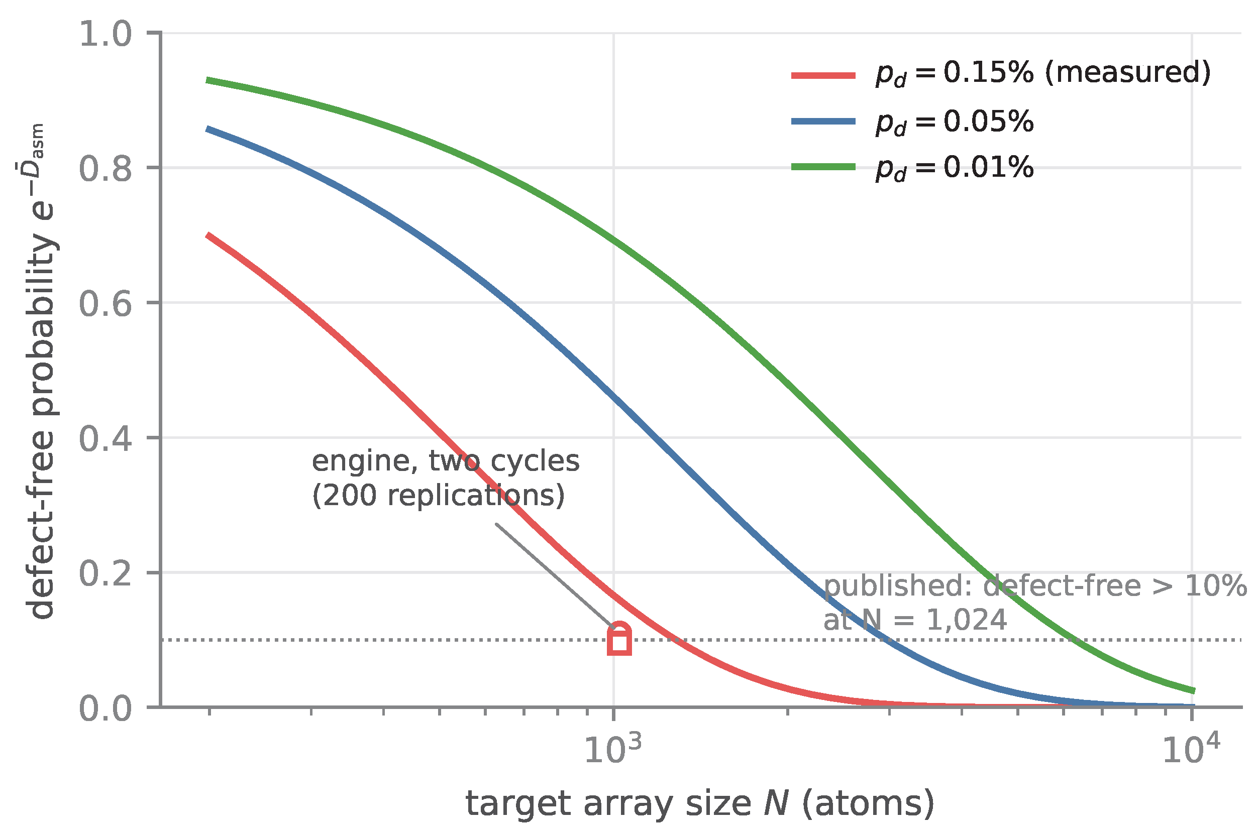
Figure 2.
The array size at which the loop loses its working point, against the number of moving beams, at and . The lines are the map (Table 4); the open marker is the engine’s cliff at one beam and (a basin at 1,000 sites, divergence at 2,000). Each doubling of the beams buys a factor in array size: a factor of two for a linear pass, 1.6 at , 1.4 for a quadratic one.
Figure 2.
The array size at which the loop loses its working point, against the number of moving beams, at and . The lines are the map (Table 4); the open marker is the engine’s cliff at one beam and (a basin at 1,000 sites, divergence at 2,000). Each doubling of the beams buys a factor in array size: a factor of two for a linear pass, 1.6 at , 1.4 for a quadratic one.
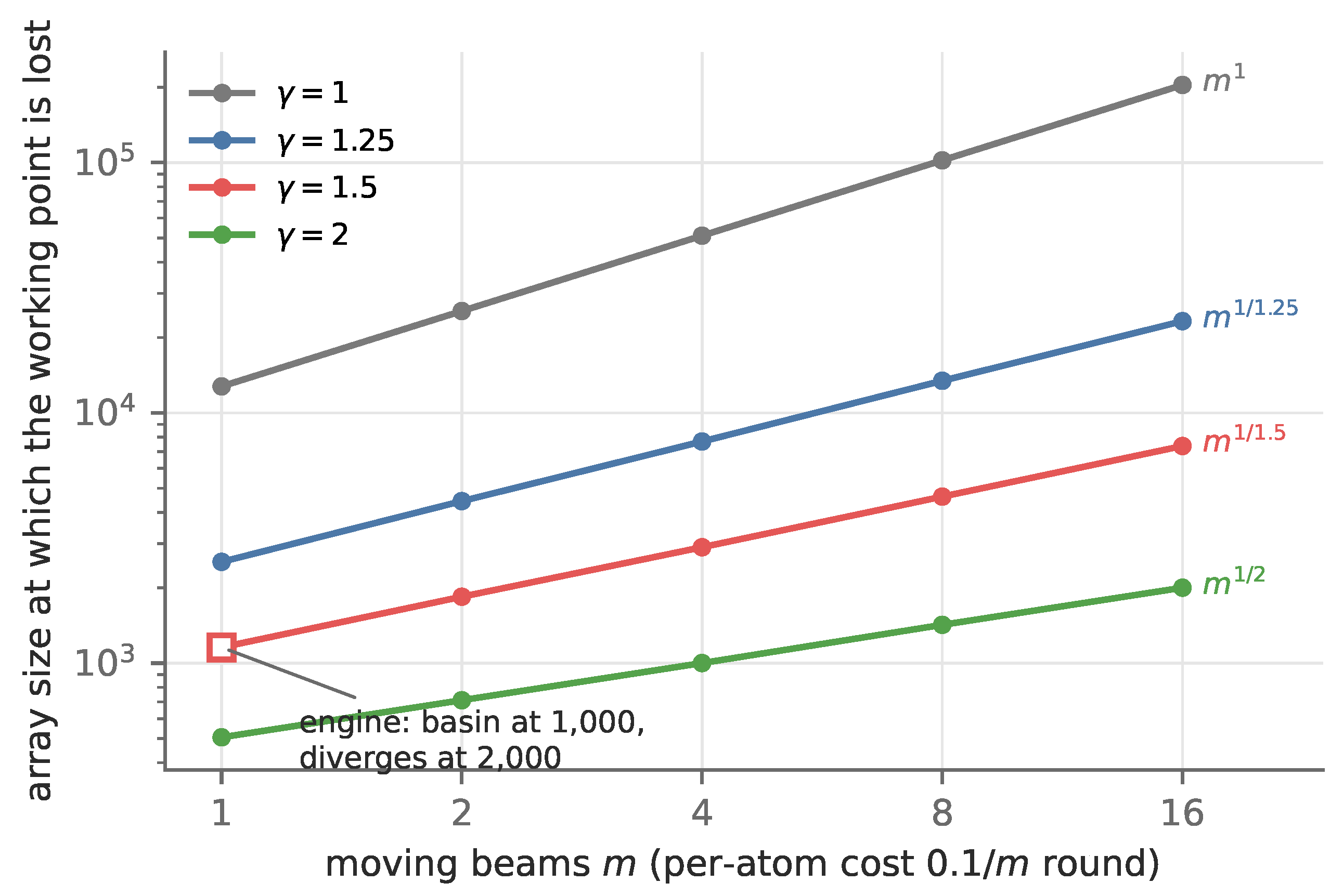

Table 1.
Shot-based assembly: residual vacancies after each vacancy pass, engine (200 replications) against the map (2), and the engine’s defect-free fraction. The rows are the experiment’s second cycle; the rows are the map’s own passes to its floor, not the experiment’s first cycle (see text). Cryogenic arm: , , , , , , or . Room-lifetime arm: , , s as reported, or 40 s. Published values [2,3] in the last column.
Table 1.
Shot-based assembly: residual vacancies after each vacancy pass, engine (200 replications) against the map (2), and the engine’s defect-free fraction. The rows are the experiment’s second cycle; the rows are the map’s own passes to its floor, not the experiment’s first cycle (see text). Cryogenic arm: , , , , , , or . Room-lifetime arm: , , s as reported, or 40 s. Published values [2,3] in the last column.
| arm | after 1 | map | after 2 | map | defect-free | published |
|---|---|---|---|---|---|---|
| cryo, , | 3.2 | 3.3 | 3.1 holes (), | |||
| cryo, , | 4.2 | 4.3 | defect-free | |||
| cryo, , | 7.3 | 7.5 | 1.9 | 1.9 | 11% | |
| cryo, , | 10.8 | 11.0 | 2.0 | 2.0 | 10% | |
| 828 atoms, s, | 17.0 | 17.4 | 14.9 | 15.1 | 0% | 41 holes () |
| 828 atoms, s, | 29.9 | 30.6 | 33.8 | 35.3 | 0% |
Table 2.
The defect-free size limit of Eq. (4) at the cryogenic background loss ( s), by per-image loss and cycle overhead. The measured point is , rounds (1.3 s).
Table 2.
The defect-free size limit of Eq. (4) at the cryogenic background loss ( s), by per-image loss and cycle overhead. The measured point is , rounds (1.3 s).
| (1.3 s) | (0.3 s) | (0.1 s) | |
|---|---|---|---|
| 560 | 630 | 650 | |
| 1,290 | 1,750 | 1,890 | |
| 2,720 | 6,130 | 8,170 |
Table 3.
The sustained loop with one moving beam: fixed, , , , greedy reload, a tolerance of , reservoir refilled at , 40 replications of 3,000 rounds, a burst of 64 vacancies at round 300. and from the map; and the crossing probability measured. The move duty is the fraction of the time the beam spends transporting.
Table 3.
The sustained loop with one moving beam: fixed, , , , greedy reload, a tolerance of , reservoir refilled at , 40 replications of 3,000 rounds, a burst of 64 vacancies at round 300. and from the map; and the crossing probability measured. The move duty is the fraction of the time the beam spends transporting.
| N | move duty | crossed (no burst) | crossed (burst 64) | ||||
|---|---|---|---|---|---|---|---|
| 1 | 500 | 5% | 5.3 | none | 0% | 0% | 8.1 |
| 1000 | 10% | 11.2 | none | 0% | 0% | 17.1 | |
| 2000 | 20% | 25.2 | none | 0% | 0% | 38.3 | |
| 4000 | 40% | 67.0 | none | 0% | 0% | 100 | |
| 8000 | 80% | 355 | none | 0% | 0% | 481 | |
| 1.5 | 500 | 5% | 5.7 | none | 0% | 0% | 9.0 |
| 1000 | 10% | 17.2 | 96 | 0% | 0% | 27.2 | |
| 2000 | 20% | sat. | sat. | 100% | 100% | 1,046 | |
| 4000 | 40% | sat. | sat. | 100% | 100% | 2,550 | |
| 8000 | 80% | sat. | sat. | 100% | 100% | 5,311 |
Table 4.
The array size at which the working point of the loop is lost, from the map, with m moving beams (), , . A working point is a stable fixed point below a quarter of the array; for it disappears in a saddle-node with , for it climbs through the quarter. The scaling with m is .
Table 4.
The array size at which the working point of the loop is lost, from the map, with m moving beams (), , . A working point is a stable fixed point below a quarter of the array; for it disappears in a saddle-node with , for it climbs through the quarter. The scaling with m is .
| p | 2 | 4 | 8 | 16 | ||
|---|---|---|---|---|---|---|
| 1 | 12,800 | 25,500 | 51,000 | 102,000 | 204,000 | |
| 1.25 | 2,540 | 4,440 | 7,680 | 13,400 | 23,200 | |
| 1.5 | 1,160 | 1,840 | 2,900 | 4,630 | 7,370 | |
| 2 | 505 | 710 | 1,000 | 1,420 | 2,000 | |
| 1 | 910 | 1,820 | 3,650 | 7,300 | 14,600 | |
| 1.25 | 310 | 540 | 930 | 1,630 | 2,850 | |
| 1.5 | 380 | 600 | 950 |
Disclaimer/Publisher’s Note: The statements, opinions and data contained in all publications are solely those of the individual author(s) and contributor(s) and not of MDPI and/or the editor(s). MDPI and/or the editor(s) disclaim responsibility for any injury to people or property resulting from any ideas, methods, instructions or products referred to in the content. |
© 2026 by the authors. Licensee MDPI, Basel, Switzerland. This article is an open access article distributed under the terms and conditions of the Creative Commons Attribution (CC BY) license (http://creativecommons.org/licenses/by/4.0/).
Copyright: This open access article is published under a Creative Commons CC BY 4.0 license, which permit the free download, distribution, and reuse, provided that the author and preprint are cited in any reuse.