

Submitted:
11 September 2026
Posted:
15 September 2026
You are already at the latest version
Abstract
Accurate short-term forecasting of photovoltaic (PV) generation, long a concern for grid operators, is increasingly relevant to prosumers as well: the households and small businesses that both produce and consume electricity and must plan storage, self-consumption, and grid export. This paper studies solar forecasting under the constraint that users rarely possess years of historical generation data that data-hungry deep models assume. We release an open-source toolkit that integrates 7 forecasting models, spanning gradient-boosted trees, recurrent and convolutional sequence models, and attention- and basis-expansion architectures. We evaluate the toolkit’s performance on a newly released dataset of two grid-connected 50 kWp PV systems in southwestern Romania, using a strict rolling-origin walk-forward protocol. Across all experiments, XGBoost and LightGBM lead: on the primary site, they achieve 10.4% normalized RMSE against 12.9% for the best deep model, and they already beat a naive persistence baseline after a single month of training data. A dedicated small-window study shows that the boosting advantage is concentrated in the cold-start regime and narrows steadily as history accumulates, from a factor of 2.1 at one month to 1.08 at twelve, with no model saturating inside the available record. A cross-site replication on a second, independent installation reproduces the full model ranking almost exactly (Spearman ρ=0.964), strong evidence that the finding is not a single-dataset artifact. The resulting forecaster is deliberately lightweight and cost-efficient: a few hundred shallow trees over a seven-feature lag/rolling core that trains in under a second per month on a commodity CPU. We publicly release the toolkit and the anonymized two-site dataset to support reproducible prosumer-scale PV forecasting research.
Keywords:
photovoltaic forecasting
; prosumer energy
; gradient boosting
; XGBoost
; cold-start
; small data
; cross-site validation
; lightweight models
; cost-efficient forecasting
; open dataset
1. Introduction
Solar photovoltaic (PV) power is the fastest-growing electricity source worldwide, accounting for the majority of new renewable capacity added in recent years [1]. A large and rising share of this capacity is distributed: PV systems owned by prosumers, households and small businesses that simultaneously generate and consume electricity. For these users, knowing how much a system will produce over the coming days directly informs battery dispatch, self-consumption scheduling, and grid-export decisions, and it does so at a scale where a dedicated forecasting service is rarely economical.
Solar generation is intermittent and stochastic, governed by cloud dynamics that are difficult to predict beyond a few hours [2,3]. Data-driven methods can learn the mapping from recent history and weather to future output without an explicit physical model, and much recent work has favored deep sequence architectures [3]. However, most of this literature assumes abundant training data. A newly commissioned PV system has no such history, and the very users who would benefit most from a forecast have the least data to train one. This cold-start regime, rather than the large-installation setting, is the practical bottleneck for prosumer forecasting.
This paper studies short-term PV forecasting under realistic prosumer constraints: single-site data, a short history, and commodity inverter exports as the only input. We make three contributions. The first is empirical. Under a strict walk-forward protocol, gradient-boosted trees beat every deep architecture we tested by 1.24× in normalized RMSE, and that margin survives each test we made to close it: a training window cut to a single month, a replication on a second installation (Spearman ), warm-start retraining, ensembling, physics-informed features, and a held-out calendar month that no training run had seen. The second contribution is explanatory. A feature-importance and recency analysis shows that the forecast rests on recent local signals, chiefly the previous hour of generation together with current irradiance, rather than on seasonal or historic context. That is why recency-weighted training helps, and why such a short history costs so little. The third contribution considers the resources. We release the toolkit and the anonymized two-site dataset, with weather and solar-geometry features already merged, together with the toolkit that produced every result reported here, at https://github.com/upb-nlp/PV-Generation-Dataset [4]. The toolkit builds the feature matrix of Section 3, implements the seven models and the three persistence baselines behind a single interface, and runs the walk-forward protocol of Section 3.3; a separate entry point issues an operational forecast from a recorded history, which is the path evaluated in Section 5.3.4. Each experiment below corresponds to one script, so the tables can be regenerated from the released data, and a new installation can be substituted for ours by pointing the same scripts at its own inverter export. Paired with the persistence baselines in Table 2, it is intended to compare forecasters on prosumer-scale data, a setting where public benchmarks remain scarce.
2. Related Work
Solar power forecasting has evolved rapidly over the past two decades, driven by advances in machine learning, the growing availability of digitized meteorological and generation data, and the urgency of integrating variable renewable energy production sources into power grids. A recent systematic review by Husein et al. [5], which screens 36 case studies published in 2022–2023, finds LSTM to be the most widely applied deep-learning technique in the field, appearing in 31 of them, followed by CNN in 21, with BiLSTM, GRU, and Transformer variants trailing well behind. The area is plainly active and fast-moving [2,3]. This section traces that evolution and identifies the gap that motivates our study.
2.1. Physical and Statistical Baselines
The earliest quantitative forecasts were grounded in physical models of solar geometry and atmospheric radiative transfer. Clear-sky models compute the theoretical maximum irradiance from geographic coordinates, date, and time of day; the PVGIS tool [6] implements this family and is widely used as a reference for simulation data. Such models are interpretable and need no historical data, but their accuracy degrades sharply under realistic cloud cover, limiting their operational value. Statistical time-series methods add a data-driven layer: autoregressive integrated moving-average (ARIMA) models and their seasonal variant (SARIMA) exploit the strong diurnal and annual autocorrelation of generation and remain common benchmarks [7], though their linearity assumption is a fundamental limitation because the irradiance-to-power relationship is non-linear, especially near inverter clipping and during rapid clear-to-cloudy transitions. Persistence models, which forecast the next period to equal the current one, are standard sanity-check baselines, with a smart variant that additionally rescales by the predicted clear-sky index [8].
2.2. Gradient Boosting and Tabular Machine Learning
Supervised learning on tabular features was adopted for its ability to model non-linear input–output relationships without explicit physical assumptions. Linear regression is the simplest learned baseline and quantifies the linearly explainable variance, but it systematically underfits solar output because both the temperature-efficiency and irradiance-to-power curves are non-linear. Gradient-boosted trees, and XGBoost [9] in particular, have become the dominant non-deep-learning approach: they build an additive ensemble of trees in which each new tree fits the residuals of the previous ensemble, capturing complex feature interactions while remaining robust to outliers and efficient on tabular data. LightGBM [10] offers a leaf-wise, histogram-based alternative with comparable accuracy and faster training. Several studies report that gradient boosting matches or exceeds shallow neural networks on PV benchmarks, especially when training data are limited: Rodriguez-Leguizamon et al. [7] report an near 0.99 for an XGBoost-based pipeline, and comparative reviews find gradient boosting to offer the best accuracy-per-training-cost among tabular learners [11]. A recent head-to-head study of XGBoost, LightGBM, and LSTM ranks the two boosting methods above the recurrent network [12], and comparative work including bidirectional LSTM variants reaches similar conclusions [13]. The shared limitation of tree methods is that they lack internal temporal state, so multi-hour dependencies must be supplied explicitly through lag and rolling features rather than learned by a recurrent mechanism, making feature engineering central to their success.
2.3. Recurrent and Convolutional Deep Networks
The prominence of LSTM networks in PV forecasting stems from their ability to model temporal sequences with long-range dependencies [14]: gating mechanisms allow the cell state to selectively retain information over many steps, mitigating the vanishing-gradient problem of plain recurrent networks. A standard (vanilla) LSTM, trained on a sliding window of past observations to predict the next step, captures the diurnal generation cycle with markedly lower error than ARIMA and SARIMA baselines, by 31% and 47% respectively on a 250 kW Indian installation [15]. A large body of work explores architectural refinements: bidirectional LSTMs process the window in both directions and have reported the lowest error among LSTM variants on some datasets [13], while stacked LSTMs build a hierarchical temporal extractor whose lower layers track short-term cloud fluctuations and upper layers encode diurnal and seasonal structure [8]. Convolutional front-ends are frequently combined with recurrence: a CNN acts as a local feature extractor that compresses the raw window and smooths high-frequency noise before the LSTM integrates it over time. CNN-LSTM hybrids outperform standalone CNN and LSTM on short-term PV production [16], and dual-stream variants that process several meteorological channels in parallel before merging them with attention report state-of-the-art results on regional datasets [17].
2.4. Attention Mechanisms and Transformers
Attention lets a model learn which positions in the input window matter most for the prediction, weighting each step rather than treating all past observations equally [18]. For PV this is valuable because midday generation is far more informative than overnight zeros. For PV, this is valuable because midday generation is far more informative than overnight zeros. Several studies add attention to recurrent backbones with consistent gains, including Bayesian-optimized CNN-BiLSTM stacks with attention weighting for high-resolution prediction [19], attention-based CNN-LSTM day-ahead forecasters [20], and spatially-downscaled attention hybrids driven by numerical weather prediction [21]. The Transformer [22] removes recurrence entirely: global self-attention gives every step a direct, constant-length path to every other, improving long-range modeling at an cost. Transformer-based PV models have grown quickly since 2022 and are reported as the most accurate family in recent surveys [5], including CNN-LSTM-Transformer hybrids [23] and encoder–decoder frameworks that pair a Transformer with a generative language model for explainable short-term prediction [24]. Dedicated forecasting architectures such as N-BEATS [25], whose stacked basis-expansion blocks learn interpretable trend and seasonality components without any recurrence, extend this line. A recurring practical concern is data hunger: self-attention needs large training sets to learn meaningful global patterns and tends to overfit on the limited history available from a single residential inverter, precisely the regime we study.
2.5. Feature Engineering
The input representation is at least as consequential as the architecture, and the literature has converged on four feature groups. Solar-position features (elevation, azimuth, clear-sky irradiance), computed deterministically from coordinates and timestamps using ephemeris libraries such as pvlib [26], define the geometric generation envelope and require no measurements. Meteorological features (irradiance, temperature, wind, cloud cover, humidity) modulate the conversion of available irradiance into power, and the stochastic behavior of cloud cover is the main obstacle to accurate forecasting [5]. Correlation-based selection of the most informative meteorological channels is a standard preprocessing step in hybrid models [23]. Temporal features (hour, day-of-year, month) appear in virtually every recent model [24], and encoding them as sine–cosine pairs preserves their periodic structure and exposes multi-scale seasonality. Finally, lag and rolling statistics make the recent trajectory explicit for non-recurrent models. Supplying them as extra channels also stabilizes LSTM predictions by anchoring the internal state to recent observations [13].
2.6. Evaluation Practice and Probabilistic Forecasting
A persistent obstacle to cross-study comparison is the absence of a standard evaluation protocol: studies differ in error metrics, normalization, and temporal aggregation, making it hard to tell whether a new model advances the state of the art or merely suits a favorable split [2,5]. We therefore report five complementary metrics (MAE, RMSE, MAPE, nRMSE, and ) uniformly, following common practice [7,13], with nRMSE as the primary capacity-normalized measure, enabling comparison across systems with different rated power. Equally important is how the data are split: random train/test partitions leak future information into the past and inflate reported accuracy, whereas rolling-origin (walk-forward) evaluation, which we adopt, respects the temporal order. Beyond point forecasts, probabilistic forecasting, providing a predictive interval rather than a single value, is increasingly recognized as the right framing for decision-making under uncertainty [2]: a battery controller needs the plausible range of outcomes, not just the mean. We leave interval estimation to future work.
2.7. Data Scarcity, Transfer Learning, and the Prosumer Gap
Because a newly commissioned system has little history, transfer learning has become a leading response to data scarcity. Sarmas et al. [8] systematically compare weight-freezing, fine-tuning, and feature-extraction strategies with a stacked-LSTM base model and find that all three outperform training from scratch on small-target datasets, improving RMSE by 12.6% with a year of training data and widening the gap further in the three-month regime. The SolNet framework [27] pre-trains a multivariate forecaster on abundant PVGIS-generated synthetic data and then fine-tunes on observations from the target inverter, with the transfer benefit strongest where observations are scarcest, across hundreds of sites in the Netherlands, Belgium, and Australia. Zhang et al. [28] show that transfer can even bridge climates, matching four months of local training with as little as two weeks of target data after a California-to-UK transfer. Most recently, foundation models have aimed at zero-shot irradiance prediction across sites without any target-site training [29]. These approaches are powerful but operationally heavy for a single prosumer, and they typically rely on large public collections such as the UK PV dataset [30] or on synthetic simulation pipelines. Comparatively little work isolates the problem we address: given only a few months of one system’s own inverter exports, establishing which model family is actually deployable, whether that choice holds up at a second site, and whether it survives changes in training strategy, feature engineering, hyperparameter tuning, and a genuinely prospective test. Existing end-user tooling does not close this gap either, as it is split between proprietary fleet platforms and research codebases that require programming expertise. We address these points directly and release the data and tooling to make the comparison reproducible.
3. Method
3.1. Corpora
Two study sites are considered for the current experiments, both grid-connected 50 kWp installations in southwestern Romania that share an inverter class but are owned and operated independently of one another. Site A supplies the primary record against which every experiment is run; Site B is held back as an independent installation used to test whether the findings survive a change of site (Section 5.3.2). Their histories are of deliberately different length, 18 months against 13, so the cross-site comparison is aligned to a common window rather than to each site’s full record.
The primary site (Site A) is a grid-connected PV system in southwestern Romania (approximately N, E; coordinates rounded to ∼11 km for anonymity), built around a Huawei SUN2000-50KTL-M0 inverter with 50 kWp of installed capacity. Raw data are 5-minute FusionSolar exports covering January 2025 to June 2026 (18 months).
The second site (Site B) is an independent installation of the same inverter class and capacity in the same region, with 13 months of history (May 2025 to May 2026, 9,336 hourly records). The two systems have different owners and locations. Site B’s exact coordinates were not disclosed, so we use Site A’s coordinates as a regional proxy, which we flag as a limitation.
Five-minute active-power readings were resampled to hourly means and normalized to the dimensionless capacity factor,
Equation 1 makes results comparable across systems of different sizes. Night hours (solar elevation below ) are excluded from all error metrics, since predicting zero output at night is trivial and would inflate apparent accuracy. Ingestion handles Huawei sentinel values and locale-specific number formatting.
Each hourly record includes the following information: (i) lagged capacity factors (, , , ); (ii) short-window rolling statistics over the three and six hours preceding the predicted hour (3-hour and 6-hour means, 3-hour standard deviation); (iii) cyclic time encodings (hour, day-of-year, month); (iv) solar-geometry features from pvlib [26] (elevation, azimuth, zenith, clear-sky GHI, and an elevation–capacity interaction term); and (v) historical weather from the Open-Meteo reanalysis (temperature, humidity, precipitation, wind, cloud cover, and short-/direct-wave radiation). This yields a 25-feature tabular representation shared by all models, extended to 28 features in the physics-informed variant of Section 5.1.2.
The two-site data are published as an anonymized, CC-BY-4.0 dataset [4]. For each site, we provide a pre-merged hourly CSV file (inverter output, Open-Meteo weather, pvlib solar position, and capacity factor) as the recommended entry point, along with the trimmed raw 5-minute exports for full pipeline reproducibility. All personally identifying fields present in the vendor exports, owner and installer names embedded in location, device, and management columns, and inverter serial numbers in filenames, were removed by rebuilding each affected field from known-safe components rather than partial editing, and coordinates were rounded to ∼11 km. A line-by-line scanner verifies that no original identifier survives in any released file.
3.2. Our Toolkit - Models and Experimental Setup
We compare 7 models spanning three families, selected so that no conclusion rests on a single implementation. How each family consumes the data varies, and the distinction matters for interpreting the results: the gradient-boosted trees map a single feature row to the capacity factor for that same hour, whereas the 5 deep models map a 24-hour input window to the capacity factor of its final hour. Both therefore predict one hour at a time. Section 3.4 sets out how those hourly predictions become the monthly figures reported throughout, and why no model is ever fed its own output; Section 5.3.4 takes the forecast out to the multi-week horizon.
The gradient-boosted trees, XGBoost [9] (depth-wise growth) and LightGBM [10] (leaf-wise growth), consume the feature tabular vector directly, with roughly a few hundred shallow trees. The recurrent and convolutional sequence models are a vanilla LSTM [14], a CNN-LSTM that prepends 1-D convolutions for local feature extraction, and an attention-augmented LSTM [18]. All three process a 24-hour input window. The attention and basis-expansion forecasters are a Transformer encoder [22] and N-BEATS [25] with its interpretable basis blocks, which represent the current state of the art for deep time-series forecasting. All deep models use a 24-step input sequence, are trained for up to 100 epochs with early stopping (patience 10) and gradient clipping, and share the feature set above. Any model that raises an exception during an iteration records a missing result for that iteration and never crashes the full comparison; XGBoost serves as the last-resort baseline.
All five deep models share a single training budget so the comparison stays fair: up to 100 Adam epochs (learning rate , batch size 64) with gradient-norm clipping at 1.0, minimizing a recency-weighted mean-squared error over the 24-hour windows. Early stopping with patience 10 restores the best-loss weights once the training loss no longer improves. We monitor training rather than validation loss inside each walk-forward fold because splitting a six- to eleven-month fold further would remove scarce data. We selected hyperparameters by grid search on a temporal validation split rather than adopting defaults: we train on the first five months of Site A and validate on the sixth month, which precedes every walk-forward test month and therefore leaks no test data. Tuning moves the tree models by roughly three quarters of a point, from 9.08% to 8.49% validation nRMSE for XGBoost and from 9.29% to 8.36% for LightGBM, both best at 300 trees of depth 4 with a learning rate of 0.03, against the held configuration of Table 1. It does not change the ranking: the strongest deep model at its best-validated width, a CNN-LSTM at width 128, reaches 10.63%, and the Transformer 11.15% at width 32, so both remain behind the boosting models even at the latter’s untuned settings. Because the gains are modest and the ordering is stable, we hold a single configuration constant across all models, sites, and experiments. The search confirms that the gradient-boosting advantage reflects the data regime rather than a hyperparameter choice.
3.3. Evaluation Protocols
We use two complementary protocols. The primary one is a rolling-origin (walk-forward) scheme that mirrors real deployment: train on months , predict month , then slide the origin forward by one month and repeat. The minimum training window is six months, yielding 12 evaluation iterations on Site A. Training samples are weighted by an exponential recency decay ( per month, 18-month cutoff). No random train/test splitting is used, which would leak future information into the past. The second protocol is a fixed-holdout test that reserves one specific calendar period as an untouched test set: it is used both for the small-window study (Section 5.1.1) and for the prospective May 2026 evaluation (Section 5.3.1), where the holdout month post-dates every training run and thus gives a genuinely out-of-sample estimate. Section 5.3.4 adds a third, operational protocol in which the model receives no observation whatsoever from the forecast period.
3.4. From Hourly Predictions to a Monthly Forecast
Every model predicts one hour at a time, so a monthly figure reported in this paper is the set of hourly predictions covering that test month, scored over its daytime hours. The prediction is a direct multi-step: no model is ever fed its own output. Within an evaluation month, the lag and rolling features for each timestamp are computed from recorded generation at earlier timestamps, which is information a deployed forecaster would hold at that moment too, so the prediction for one hour never depends on the prediction for the hour before it, and nothing from the present or future enters the feature row.
The lag and rolling features are read from measured generation, so they can only be built for hours that have already been recorded. A forecast that extends past the end of the available history loses exactly that: predicting hour t requires , but hour has not occurred yet, so there is no measurement to read. We therefore seed all four lag features ( hours) and the rolling statistics from climatology, using the historical mean capacity factor for the same calendar month and hour of day; we compute solar geometry exactly at every future timestamp, which is possible because it depends only on the date and the site’s coordinates rather than on any observation; and we clip negative capacity-factor predictions to zero before converting to kW. Section 5.3.4 evaluates that operational path directly against recorded generation.
3.5. Evaluation Metrics
We report 5 performance metrics on daytime hours: mean absolute error (MAE, kW), root mean squared error (RMSE, kW), mean absolute percentage error (MAPE, %), normalized RMSE (nRMSE, as a percentage of the 50 kWp rated capacity), and the coefficient of determination . nRMSE is our primary metric because it is directly comparable across sites of different sizes.
3.6. Use of Generative Artificial Intelligence
Generative Artificial Intelligence (AI) tools were used during the preparation of this work to assist with text generation based on concepts, ideas, and scientific content provided by the authors, and the implementation and refinement of code. All AI-generated outputs were reviewed, edited, and, where applicable, validated by the authors.
4. Results
Table 3 reports results from the 7 models integrated in our toolkit on Site A. Gradient boosting leads: LightGBM (10.39% nRMSE) and XGBoost (10.59%) are statistically indistinguishable and beat the best deep model (Transformer, 12.88%) by a factor of 1.24. The remaining deep models cluster near the naive persistence baseline (15.54%, Table 2): the vanilla LSTM (15.48%) and CNN-LSTM (15.43%) are statistically indistinguishable from it, while the attention-LSTM (16.47%) and N-BEATS (17.12%) fall behind it. Because a depth-wise (XGBoost) and a leaf-wise (LightGBM) implementation land within 0.2 points of each other, the advantage is a property of the gradient-boosting family, not of one implementation. Pairwise Wilcoxon tests against the vanilla LSTM confirm the ordering is significant for both tree models ().

Table 2.
Persistence baselines on Site A (walk-forward).
| Baseline | nRMSE | MAE (kW) | |
|---|---|---|---|
| Naive persistence | 15.54% | 5.74 | 0.724 |
| Day persistence | 26.94% | 8.75 | 0.098 |
| Smart persistence | 26.96% | 8.75 | 0.096 |
Table 3.
A comparison using our toolkit with 7 models run on Site A, averaged over 12 walk-forward iterations. Lower nRMSE/MAE and higher are better. The p column reports a Wilcoxon signed-rank test on per-iteration nRMSE against the vanilla LSTM.
Table 3.
A comparison using our toolkit with 7 models run on Site A, averaged over 12 walk-forward iterations. Lower nRMSE/MAE and higher are better. The p column reports a Wilcoxon signed-rank test on per-iteration nRMSE against the vanilla LSTM.
| Rank | Model | nRMSE | MAE (kW) | p | |
|---|---|---|---|---|---|
| 1 | LightGBM | 10.39% | 3.38 | 0.875 | 0.0005 |
| 2 | XGBoost | 10.59% | 3.48 | 0.870 | 0.0005 |
| 3 | Transformer | 12.88% | 4.53 | 0.805 | 0.0005 |
| 4 | CNN-LSTM | 15.43% | 5.53 | 0.702 | 0.380 |
| 5 | Vanilla LSTM | 15.48% | 5.54 | 0.703 | — |
| 6 | Attention-LSTM | 16.47% | 5.79 | 0.664 | 0.043 |
| 7 | N-BEATS | 17.12% | 5.89 | 0.627 | 0.003 |
The root cause is the temporal structure of PV output combined with the size of the training set. On a single site, generation is dominated by sun position (deterministic) and short-window cloud persistence, both of which the lag and rolling features encode directly. With only ∼6,000 daytime training rows, the deep models have too little data to regularize their larger parameter counts, while the boosted trees exploit the tabular autocorrelation structure efficiently. The margin is nonetheless far smaller than the accuracy of the tree models alone would suggest, and Section 5.1.1 shows that it is largely a small-data effect.
5. Discussion
Building on the previously reported model performance, we measure how much historical information the models actually need, which features drive the forecast, test whether warm-starting or ensembling narrows the gap, check the ranking on an unseen month and at a second site, and finally take the forecaster out to a horizon where it receives no observations at all. The margin reported above rests on one site, one training window, and one feature set, and each experiment below attempts to overturn it.
5.1. Data and Feature Requirements
5.1.1. Training Windows Requirements
For prosumers, the decisive question is not peak accuracy but how quickly a model becomes useful. Table 4 and Figure 1 show nRMSE on a fixed three-month holdout as the training window grows from one to twelve months. XGBoost improves from 14.52% at one month to 12.70% at six and 11.35% at twelve, and it beats naive persistence (17.43%) at every window, including the first. A newly commissioned site therefore reaches useful forecasting immediately and continues to improve, and no model has flattened by the end of the available record.
The deep models behave very differently in this regime. The Transformer starts at 30.69% with one month of data, more than twice the error of gradient boosting, and improves monotonically to 12.21% at twelve months, at which point it trails XGBoost by less than a point. Its limitation is therefore one of data volume rather than architecture. For a prosumer this means that gradient boosting is the right choice from commissioning, and that a deep model only becomes worth considering once a site has accumulated more than a year of history.
5.1.2. Feature Analysis
Figure 2 ranks the features by XGBoost gain importance, thereby making the model’s reasoning explicit; Appendix A defines all considered features. Its attention is concentrated on recent generation: the previous hour’s capacity factor alone contributes 53.1% of total gain, and the three-hour rolling mean and standard deviation add a further 22.9%. Among weather inputs, the strongest are direct and global horizontal irradiance (4.2% and 3.3%), nowcasts of present sky conditions, whereas the seasonal and calendar encodings that represent long-range historic context (month_*, doy_*) contribute almost nothing (each below 0.3%). In other words, the prediction depends on the current state of the system and the sky. This is the first evidence of a recurring theme (Section 5.2): recent conditions outweigh historical ones.
Table 5 reports a feature-group ablation on XGBoost, zeroing one group at a time and retraining from scratch. Removing the four lag features raises nRMSE from 10.51% to 11.66%, the largest single effect; removing the three rolling statistics or the seven raw weather features costs about 0.2 points each. No group is individually decisive: the model draws on several partly redundant descriptions of recent conditions, so losing any one of them is largely absorbed by the others. Removing the physics-derived group slightly improves accuracy (), and the time and solar-geometry encodings are worth a few hundredths of a point. Taken one group at a time, the table understates what the non-core features are worth. Zeroing weather, solar geometry, time and physics separately costs 0.20 points in total, yet dropping all four at once, which is what the seven-feature lag and rolling core amounts to, costs about 1.4 points (Section 5.4). Each group is expendable only while the others remain to cover for it. Recent generation still carries the forecast, and the one-hour lag carries most of it, but the weather and geometry inputs earn their place, and that only becomes visible when they are removed together.
A natural hypothesis is that weather helps more when the physics is encoded explicitly rather than supplied as raw measurements. We add three derived features, a temperature-efficiency factor (IEC 61215 derating, C), a cloud-transmission factor, and a clear-sky index (actual over clear-sky irradiance), growing the set from 25 to 28, and re-run the full bake-off. The result (Table 6) is a small, uniform gain. The tree models barely move (XGBoost , LightGBM ): they already recover the same thresholds from raw inputs via splits, so an explicit monotone transform of an existing feature is largely redundant. The deep models benefit more, the Transformer most (13.56% to 12.88%, relative), because the clear-sky index provides its attention mechanism with a precomputed irradiance signal it would otherwise have to reconstruct. Feature utility is thus architecture-dependent, but the effect is modest and does not change the ranking.
5.2. Training and Ensembling Strategies
The feature importance in Section 5.1.2 shows that recent, local signals win out over seasonal ones within a single fit. The same principle is applied across the training set. Rather than treating every historical row equally, we weight each sample by an exponential recency decay, , where m is its age in months, with a hard 18-month cutoff, so the most recent months dominate the fit while older data is retained only as a weak prior. This encodes a physical fact the feature importance already hinted at: a PV system’s near-term output is governed by its current weather regime and recent operating state (seasonal sun angle, soiling, any partial shading), not by what it produced a year earlier. Historic data is useful for coverage of rare conditions, but recent data is more predictive, and the model is told so explicitly. Section 5.3.5 tests whether the same principle can be pushed further, into a multiplicative correction of long-range forecasts, and finds that it cannot.
Because the walk-forward protocol retrains at every origin, the retraining strategy itself is a design choice. We compare training each iteration from scratch against warm-starting from the previous iteration’s weights (for deep models) or continuing to add trees (for boosting). Table 7 shows a clear divergence based on model family. Warm-starting helps the Transformer, cutting nRMSE from 13.25% to 12.54% (a 5.4% relative gain), as it carries forward learned representations of generation patterns rather than relearning them each month from a few thousand rows. The gain is small enough not to matter in practice, so a Transformer trained from scratch is a close substitute for a warm-started one. For gradient boosting the effect reverses: warm-start is worse than scratch (XGBoost , LightGBM ), because appending trees trained on an earlier window creates a distribution mismatch with the current one. The practical rule is therefore model-family dependent: retrain boosting from scratch, but warm-start deep models when a stateful pipeline is available. Even so, the best warm-started deep model (12.54%) remains behind scratch gradient boosting (10.39%).
A strong tree model alongside a weaker deep model is the classic case for an ensemble, so we test whether any combination beats either member alone. We combine XGBoost, LightGBM, and the warm-started Transformer using simple averaging, inverse-nRMSE weighting, and ridge-regression stacking (Table 8). Only stacking beats the best individual model, reaching 10.35% versus LightGBM’s 10.39%, a margin of 0.035 points, or roughly 2 W of MAE on a 50 kWp system. Both averaging variants are worse than the best member, even though the three members are now of comparable skill and inverse-error weighting assigns them nearly equal weights (0.355, 0.359, 0.286). The reason is correlation rather than skill disparity: the two tree models make highly similar errors, so averaging them with a third, independent but larger error source adds variance without diversification. A stacking gain of this size does not justify running and maintaining three models, so we deploy a single gradient-boosted model.
5.3. Generalization and Operational Validation
5.3.1. Prospective Evaluation: the May 2026 Holdout
All results so far use historical data in a rolling-origin protocol. A complementary test is a month that did not exist when the models were built. We hold out May 2026 entirely, train every model on January 2025–April 2026, and predict the unseen month. Figure 3 reports the outcome. The ranking from the historical experiments holds under this genuinely prospective test: LightGBM (11.41%) and XGBoost (11.60%) lead, the Transformer follows at 12.25% (), and the remaining deep models trail between 13.4% and 16.2%. Every model, including N-BEATS, beats the naive persistence baseline of 17.50% on this month.
This is also the narrowest margin recorded anywhere in the study: 0.84 points, a factor of 1.07, between the best tree model and the best deep model. It is likewise the experiment with the most training data, sixteen months, which is consistent with the small-window analysis of Section 5.1.1: the gradient-boosting advantage is largely an advantage under data scarcity, and it erodes as a site accumulates history.
5.3.2. Dual-Site Validation
All results so far are from the first site. A single-site study, however thorough, invites the objection that gradient boosting merely fits one system’s idiosyncrasies, so we now lean on a second, independent installation (Site B) to test whether the picture generalizes. This is where the small-data regime directly shapes the analysis. Site B has only 13 months of history against Site A’s 18, so a fair comparison cannot use each site’s full record; comparing Site A’s full-history results to a fresh Site B bake-off would confound the site difference with different calendar months and different amounts of walk-forward training growth. We therefore re-run Site A restricted to Site B’s exact window (train May–October 2025, test November 2025–May 2026), so both sites share identical, and deliberately short, train/test splits.
Table 9 and Figure 4 report the aligned comparison. Two things follow. First, because both sites are now trained on roughly five months rather than their full history, the leading models score higher than in Table 3 (XGBoost 10.70% aligned vs 10.59% full-history): the dual-site validation is itself run in the small-data regime this paper is about, and gradient boosting’s tolerance of short windows (Section 5.1.1) is what keeps the comparison meaningful at all. Second, and despite that, the ranking is preserved almost perfectly: the top five places are identical at both sites, and only one adjacent pair exchanges positions, N-BEATS with the attention-LSTM. The Spearman rank correlation between the two orderings is (, Figure 5). Gradient boosting leads at both sites, and the gradient-boosting-to-Transformer gap is 1.38× at Site A and 1.32× at Site B, consistent across installations. Site B is uniformly easier to forecast; all models score a lower nRMSE there, and because the gap is consistent across all architectures rather than concentrated in one, it points to a lower site noise floor (fewer logger dropouts, shading, or soiling) rather than a model-capability difference. This replication is the strongest evidence in the study that the gradient-boosting advantage is a property of prosumer-scale, small-window PV data, not of one installation.
5.3.3. Deployment Validation on Both Sites
The dual-site bake-off ranks all seven models, whereas deployment poses a narrower and more useful test, namely whether the deployed model remains accurate month after month at each site. We run the production XGBoost model in walk-forward over each site’s full history and report the per-iteration nRMSE in Figure 6. Site A averages 10.6% over 12 successive test months (July 2025–June 2026) and Site B averages 9.6% over 7 (November 2025–May 2026); the per-month range is 7.4–12.3% at Site A and 6.8–12.9% at Site B, and every month at both sites stays below the naive persistence baseline. Site A’s 10.6% here agrees with the full-history XGBoost figure of Table 3, computed over the same twelve iterations; the model degrades gracefully rather than drifting, and its month-to-month variation tracks weather regime rather than time since the last retrain.
5.3.4. Forecasting Without Observations: The Operational Horizon
The walk-forward protocol supplies each test hour with lag features drawn from recorded generation an hour earlier, which is what a live system holds when it forecasts the next hour but not what it holds when a prosumer asks for the coming fortnight. We therefore run the deployment path directly: train on January 2025–April 2026, then forecast the 61 days of May and June 2026 with no access to generation in that period at all. Lag and rolling inputs are seeded from climatology, weather is supplied for the first 14 days and taken from climatology thereafter. The weather supplied in this first experiment is the reanalysis, that is, the weather that actually occurred, which bounds what any weather input could contribute; the lead-time experiment below replaces it with real archived forecasts.
Table 10 reports the outcome against recorded output. Over the fortnight with known weather the forecaster reaches 14.51% nRMSE, against 18.95% for a pure climatological forecast over the same days: the model adds 4.4 points of skill at that horizon. Beyond it, where both weather and lags come from climatology, the model retains a small edge (16.43% against 16.72%). Accuracy does not decay monotonically with horizon; it tracks the weather regime of each week, ranging from 10.1% to 26.0% across the nine weeks (Figure 7). These are the numbers a prosumer actually experiences, and they are substantially higher than the one-hour-ahead figures of Table 3, which is the expected consequence of removing the most informative input the model has.
5.3.5. How Old May the Weather Forecast Be?
Because the reanalysis input used above describes the weather that actually occurred rather than any prediction of it, we repeated the experiment with archived numerical weather predictions from the Open-Meteo historical forecast archive, taking for each hour the value issued by the model run L days earlier, for ; the archive does not retain runs older than seven days, which caps the sweep there. Table 11 and Figure 8 report the outcome over the same May–June 2026 horizon, with weather from the given source supplied throughout.
The penalty for using a real forecast rather than the weather that occurred is small at short lead, since the day-ahead input yields 14.91% nRMSE over the first fortnight against 14.51% for the reanalysis. Skill then decays as the input ages, and by seven days the weather-driven forecast (19.43%) has converged on the forecast that uses no weather at all (19.70%), so a week-old irradiance prediction carries no more information about this site’s output than its own seasonal average does. The crossover sits near five days and tracks the error of the weather input itself, whose global horizontal irradiance RMSE against the reanalysis grows from 99 W/m2 at three days to 142 W/m2 at five.
Locating that boundary from data rather than by assumption matters for how the two forecast paths are combined, because running the model on live weather is worthwhile only while that guidance is younger than roughly five days, and beyond it the climatological path performs the same. The 16-day live-weather window offered by public forecast providers is therefore considerably wider than the horizon over which weather input actually improves a PV forecast at this site.
We also tested a recency correction on this path: the ratio of recent to climatological output over the trailing 30 days, clipped to and applied multiplicatively to the climatological portion of the forecast. Swept over 19 forecast origins across both sites, it helps in 6 and hurts in the rest, with a mean effect of points at Site A and at Site B, and a spread from to points (Figure 9). On the May 2026 horizon specifically it costs 3.4 points, because a trailing factor of 1.24 estimated from an unusually sunny May was extrapolated into a June that regressed to the norm. We therefore do not recommend the correction: a trailing 30-day window is too short to distinguish a persistent regime shift from ordinary weather variability, and the resulting multiplier overshoots as often as it helps.
5.4. Implications for Deployment
Across all previous experiments, the conclusion is consistent: on prosumer-scale single-site PV data, gradient boosting is the strongest family; deep models and richer features do not overturn it and our results are replicated at a second site and on an unseen month. Three compounding factors explain the ordering. Data volume: 6,000–10,000 daytime rows are too few to regularize deep models with tens of thousands of parameters, whereas a few hundred shallow trees fit comfortably. Temporal structure: solar output is driven by deterministic sun position and short-window cloud persistence, both captured directly by lag and rolling features, leaving less residual structure for sequence models to exploit. Feature subsumption: those same tabular features pre-compute part of the recurrent state an LSTM would otherwise learn. The margin is nonetheless modest, and Section 5.1.1 shows it narrowing as history accumulates, so the recommendation below is a claim about the cold-start regime rather than about model families in general.
The experiments converge on a single, deliberately minimal recommendation. The recommended forecaster is a gradient-boosted model over the full 28-feature set, retrained from scratch each period. This choice is dictated by the evidence: it is the most accurate model (Section 4), it is usable from the first month of data (Section 5.1.1), and it holds near 10% nRMSE month after month at both sites (Section 5.3.3). Restricting it to the seven-feature lag and rolling core costs 1.4 points (11.83% against 10.39%), so the weather and geometry inputs are worth keeping.
Accuracy aside, the main argument for this recommendation is the cost. Each monthly retrain is a few hundred shallow trees over 4,000–10,000 daytime rows and completes in well under a second on a commodity CPU (0.4–1.0 s per walk-forward iteration in our runs), with no GPU, no large parameter store, and a model that serializes to a few hundred kilobytes. It needs no site-specific physical model or configuration (tilt, azimuth, module curves), only the system’s own inverter history and a public weather feed. By contrast, the deep models we evaluated require one to two orders of magnitude more parameters, benefit from GPUs, and do not reach gradient boosting’s accuracy in this data regime. For a distributed fleet of PV systems, this difference is the difference between a forecaster that can run per-site on trivial hardware and one that cannot.
The practical payoff follows from the operational numbers rather than the benchmark ones. At 14.5% nRMSE over a fortnight with forecast weather, and 3.4 kW MAE at the one-hour horizon, the forecast is accurate enough to schedule battery charging, time grid export against price signals, or shift flexible loads with a realistic expectation of error, at a compute and data cost small enough to deploy at the scale of individual PV systems. It is not accurate enough to be treated as a firm commitment of delivered energy, and any downstream controller should be sized for the error band reported in Table 10. Section 5.3.5 adds one further operating rule, which is to fetch weather guidance no older than about five days, since beyond that the climatological path performs the same and the extra data brings no benefit.
5.5. Limitations
The main limitation concerns scope. Both sites share a climate region and a single inverter class, so the replication does not establish transfer across climates or system sizes. All experiments use hourly resolution; intra-hour forecasting may narrow the deep-model gap further. The reanalysis-driven figure of Section 5.3.4 is a perfect-weather bound, and although Section 5.3.5 puts the gap to an operational feed at 0.4 points for day-ahead guidance, the forecast archive retains model runs for only seven days, so longer lead times could not be tested and the behaviour of the weather-driven path over the second week of a fortnight forecast remains unmeasured. And while transfer learning was out of scope here, pre-training a deep model across many prosumer sites remains a promising route to eventually matching gradient boosting in the cold-start regime, precisely the gap the released dataset is intended to help close.
6. Conclusions and Future Work
We studied short-term PV forecasting under the constraints that actually bind prosumers: a single site, limited history, and commodity inverter data. The conclusion is consistent across our seven-model comparison integrated in our toolkit, a small-training-window study, a feature ablation, a retraining strategy and ensemble analysis, a physics-feature experiment, a cross-site replication, a fully prospective test on an unseen month, and a multi-week operational forecast. Gradient-boosted trees lead deep sequence models by 1.24× on real PV data, are usable from the first month of history, and derive their skill from the short-window autocorrelation captured by lag and rolling features. Neither warm-start retraining nor averaging ensembles nor richer features overturn the ordering: warm-start and physics features help only deep models, and stacking beats solo boosting, but by a margin far too small to justify its cost. The ranking replicates almost exactly at a second, independent installation () and on a held-out May 2026 (LightGBM 11.41%, XGBoost 11.60%); the deployed model holds near 10% nRMSE every month at both sites, and reaches 14.5% over a fortnight forecast with no observations from the horizon, or 14.9% when driven by a real day-ahead weather forecast rather than the realised weather. Weather guidance stops adding value at about five days of lead, beyond which a climatological input performs identically. The advantage is above all a small-data advantage, a factor of 2.1 with one month of history and 1.08 with twelve, and it has not vanished by the end of the record but is clearly eroding. This study yields a practical recommendation: a lightweight, cost-efficient gradient-boosted forecaster that trains in under a second per month on a CPU. We also release the toolkit and the anonymized two-site dataset to support reproducible prosumer-scale research.
We consider three directions for future research. The first is simply to expand the current timeframes. The small-window curves have not flattened at twelve months, so the crossover point at which a deep model would overtake gradient boosting, if one exists, lies beyond the current record; a second full year at each site would locate it, and would also extend the lead-time analysis of Section 5.3.5 across more forecast origins. The second improvement targets probabilistic output. Everything reported here is a point forecast, yet a prosumer sizing a battery needs an interval, and the walk-forward protocol already produces the per-iteration error distribution against which such intervals would be calibrated; the horizon-dependent error of Section 5.3.4 suggests the interval should widen with weather uncertainty rather than with horizon alone. The third is the transfer-learning approach noted in Section 5.5. Pre-training a deep model across many prosumer installations and fine-tuning it on a few weeks of local history is the one approach we would expect to challenge the ranking reported here, and testing it requires multiple sites rather than two. The released dataset is a first step in that direction, and it can grow as far as owners agree to share their exports.
Author Contributions
Conceptualization, N.-R.L., T.-E.R. and M.D.; methodology, N.-R.L.; software, N.-R.L.; validation, N.-R.L., T.-E.R., M.D. and S.R.; formal analysis, N.-R.L.; investigation, N.-R.L.; data curation, N.-R.L.; writing—original draft preparation, N.-R.L.; writing—review and editing, T.-E.R., S.R. and M.D.; visualization, N.-R.L.; supervision, T.-E.R. and M.D. All authors have read and agreed to the published version of the manuscript.
Funding
Not applicable.
Institutional Review Board Statement
Not applicable.
Informed Consent Statement
Not applicable.
Data Availability Statement
The dataset generated and analyzed in this study is publicly available at https://github.com/upb-nlp/PV-Generation-Dataset under a CC-BY-4.0 license [4].
Acknowledgments
During the preparation of this manuscript/study, the author(s) used Claude (Anthropic, Claude Opus 4.8+) for the purposes of generating and refining text based on the authors’ original ideas and assisting with code implementation. The authors have reviewed and edited the output and take full responsibility for the content of this publication.
Conflicts of Interest
The authors declare no conflicts of interest.
Appendix A. Feature Reference
Table A1 defines every column of the 28-feature matrix, grouped as in the ablation of Section 5.1.2. Solar geometry is recomputed with pvlib [26] from the released rounded coordinates, and the weather columns come from the Open-Meteo reanalysis already merged into the released hourly files. denotes the capacity factor of Equation 1, and t the hour being predicted. The 25-feature variant of Section 5.1.2 is this set without the physics-derived group; the seven-feature core is the lag and rolling groups alone.
Table A1.
The 28 features, by group. Every input can be computed from information available strictly before hour t, or from the calendar and the site coordinates.
Table A1.
The 28 features, by group. Every input can be computed from information available strictly before hour t, or from the calendar and the site coordinates.
| Feature | Definition |
|---|---|
| Solar geometry (5) | |
| solar_elevation_deg | Sun elevation above the horizon at t, clipped at zero. |
| solar_azimuth_deg | Sun azimuth at t, measured clockwise from north. |
| solar_zenith_deg | Sun zenith angle at t, the complement of elevation. |
| clearsky_ghi_wm2 | Clear-sky global horizontal irradiance at t (W/m2), the irradiance expected with no cloud. |
| elevation_x_capacity | Elevation scaled by rated capacity, , which equals at the zenith and zero at the horizon. |
| Weather (7), Open-Meteo reanalysis | |
| temp_c | Ambient air temperature at 2 m (∘C). |
| humidity_pct | Relative humidity (%). |
| cloud_cover_pct | Total cloud cover (%). |
| wind_speed_kmh | Wind speed at 10 m (km/h), which affects module cooling. |
| ghi_wm2 | Global horizontal irradiance (W/m2). |
| dni_wm2 | Direct normal irradiance (W/m2). |
| dhi_wm2 | Diffuse horizontal irradiance (W/m2). |
| Cyclic time encodings (6) | |
| hour_sin, hour_cos | sin and cos of for hour of day h, a pair with no discontinuity at midnight. |
| doy_sin, doy_cos | sin and cos of for day of year d. |
| month_sin, month_cos | sin and cos of for month m. |
| Capacity-factor lags (4) | |
| cf_lag_1h | , the capacity factor one hour earlier. |
| cf_lag_2h | , two hours earlier. |
| cf_lag_3h | , three hours earlier. |
| cf_lag_6h | , the longest lag in the set. |
| Rolling statistics (3) | |
| cf_roll3h_mean | Mean of over to . |
| cf_roll3h_std | Standard deviation of over to , a measure of recent variability. |
| cf_roll6h_mean | Mean of over to . |
| Physics-derived (3) | |
| temp_efficiency_factor | IEC 61215 temperature derating, with C, clipped to . |
| cloud_transmission | Fraction of irradiance transmitted through cloud, for cloud cover c, clipped to . |
| clearsky_index | Ratio of measured to clear-sky irradiance, clipped to , a dimensionless measure of sky clearness. |
References
- International Energy Agency. Renewables 2023: Analysis and Forecast to 2028. Technical report, IEA, Paris, France, 2023. IEA: Paris, France.
- Ahmed, R.; Sreeram, V.; Mishra, Y.; Arif, M.D. A review and evaluation of the state-of-the-art in PV solar power forecasting: Techniques and optimization. Renew. Sustain. Energy Rev. 2020, 124, 109792. [Google Scholar] [CrossRef]
- Kumari, P.; Toshniwal, D. Deep learning models for solar irradiance forecasting: A comprehensive review. J. Clean. Prod. 2021, 318, 128566. [Google Scholar] [CrossRef]
- Linca, N.R.; Rebedea, T.E.; Ruseti, S.; Dascalu, M. Two-site solar PV inverter and weather dataset (Romania) andToolkit. GitHub repository. 2026. Available online: https://github.com/upb-nlp/PV-Generation-Dataset.
- Husein, M.; Gago, E.J.; Hasan, B.; Pegalajar, M.C. Towards energy efficiency: A comprehensive review of deep learning-based photovoltaic power forecasting strategies. Heliyon 2024, 10, e33419. [Google Scholar] [CrossRef]
- European Commission Joint Research Centre. PVGIS: Photovoltaic Geographical Information System. 2023. Available online: https://re.jrc.ec.europa.eu/pvg_tools/en/.
- Rodriguez-Leguizamon, C.K.; López-Sotelo, J.A.; Cantillo-Luna, S.; López-Castrillón, Y.U. PV power generation forecasting based on XGBoost and LSTM models. In Proceedings of the 2023 IEEE Workshop on Power Electronics and Power Quality Applications (PEPQA), 2023; pp. 1–6. [Google Scholar] [CrossRef]
- Sarmas, E.; Dimitropoulos, N.; Marinakis, V.; Mylona, Z.; Doukas, H. Transfer learning strategies for solar power forecasting under data scarcity. Sci. Rep. 2022, 12, 14643. [Google Scholar] [CrossRef]
- Chen, T.; Guestrin, C. XGBoost: A scalable tree boosting system. In Proceedings of the Proceedings of the 22nd ACM SIGKDD International Conference on Knowledge Discovery and Data Mining, 2016; pp. 785–794. [Google Scholar] [CrossRef]
- Ke, G.; Meng, Q.; Finley, T.; Wang, T.; Chen, W.; Ma, W.; Ye, Q.; Liu, T.Y. LightGBM: A highly efficient gradient boosting decision tree. Proc. Adv. Neural Inf. Process. Syst. 2017, Vol. 30, 3146–3154. [Google Scholar]
- Mollasalehi, A.; Farhadi, A. Solar and wind power forecasting: A comparative review of LSTM, random forest, and XGBoost models. arXiv 2025, arXiv:2509.24059. [Google Scholar] [CrossRef]
- Vargas, J.; Martínez, R.; Loo, L. Enhancing photovoltaic energy forecasting with machine learning: A comparison study of XGBoost, LightGBM and LSTM models. In Proceedings of the 2024 IEEE Latin American Conference on Computational Intelligence (LA-CCI), 2024; pp. 1–6. [Google Scholar] [CrossRef]
- Alizadegan, H.; Radmehr, A.; Karimi, H.; Asghari Ilani, M. Solar energy production forecasting: A comparative study of Bi-LSTM, LSTM, XGBoost models with activation function analysis. Preprints.org 2024, 2024050994. [Google Scholar] [CrossRef]
- Hochreiter, S.; Schmidhuber, J. Long short-term memory. Neural Comput. 1997, 9, 1735–1780. [Google Scholar] [CrossRef]
- Sharma, J.; Soni, S.; Paliwal, P.; Saboor, S.; Chaurasiya, P.K.; Sharifpur, M.; Khalilpoor, N.; Afzal, A. A novel long term solar photovoltaic power forecasting approach using LSTM with Nadam optimizer: A case study of India. Energy Sci. Eng. 2022, 10, 2909–2929. [Google Scholar] [CrossRef]
- Agga, A.; Abbou, A.; Labbadi, M.; El Houm, Y.; Ou Ali, I.H. CNN-LSTM: An efficient hybrid deep learning architecture for predicting short-term photovoltaic power production. Electr. Power Syst. Res. 2022, 208, 107908. [Google Scholar] [CrossRef]
- Alharkan, H.; Habib, S.; Islam, M. Solar power prediction using dual stream CNN-LSTM architecture. Sensors 2023, 23, 945. [Google Scholar] [CrossRef]
- Bahdanau, D.; Cho, K.; Bengio, Y. Neural machine translation by jointly learning to align and translate. In Proceedings of the International Conference on Learning Representations (ICLR), 2015. [Google Scholar]
- Miraftabzadeh, S.M.; Longo, M. High-resolution PV power prediction model based on the deep learning and attention mechanism. Sustain. Energy Grids Netw. 2023, 34, 101025. [Google Scholar] [CrossRef]
- Qu, J.; Qian, Z.; Pei, Y. Day-ahead hourly photovoltaic power forecasting using attention-based CNN-LSTM neural network embedded with multiple relevant and target variables prediction pattern. Energy 2021, 232, 120996. [Google Scholar] [CrossRef]
- Peng, F.; Tang, X.; Xiao, M. Attention-enhanced CNN-LSTM with spatial downscaling for day-ahead photovoltaic power forecasting. Sensors 2026, 26, 593. [Google Scholar] [CrossRef]
- Vaswani, A.; Shazeer, N.; Parmar, N.; Uszkoreit, J.; Jones, L.; Gomez, A.N.; Kaiser; Polosukhin, I. Attention is all you need. Proc. Adv. Neural Inf. Process. Syst. 2017, Vol. 30, 5998–6008. [Google Scholar]
- Al-Ali, E.M.; Hajji, Y.; Said, Y.; Hleili, M.; Alanzi, A.M.; Laatar, A.H.; Atri, M. Solar energy production forecasting based on a hybrid CNN-LSTM-Transformer model. Mathematics 2023, 11, 676. [Google Scholar] [CrossRef]
- Siddiqa, A.; Rana, N.; Khan, W.Z.; Jeribi, F.; Tahir, A. Explaining solar forecasts with generative AI: A two-stage framework combining transformers and LLMs. PLoS ONE 2025, 20, e0331516. [Google Scholar] [CrossRef]
- Oreshkin, B.N.; Carpov, D.; Chapados, N.; Bengio, Y. N-BEATS: Neural basis expansion analysis for interpretable time series forecasting. In Proceedings of the International Conference on Learning Representations (ICLR), 2020. [Google Scholar]
- Holmgren, W.F.; Hansen, C.W.; Mikofski, M.A. pvlib python: A python package for modeling solar energy systems. J. Open Source Softw. 2018, 3, 884. [Google Scholar] [CrossRef]
- Depoortere, J.; Driesen, J.; Suykens, J.; Kazmi, H.S. SolNet: Open-source deep learning models for photovoltaic power forecasting across the globe. Int. J. Forecast. 2025, 41, 1223–1236. [Google Scholar] [CrossRef]
- Zhang, L.; Wilson, R.; Sumner, M.; Wu, Y. Transfer learning in very-short-term solar forecasting: Bridging single site data to diverse geographical applications. Appl. Energy 2025, 377, 124353. [Google Scholar] [CrossRef]
- Mishra, A.; Ravindra, T.; Iyengar, S.; Kalyanaraman, S.; Kumaraguru, P. SPIRIT: Short-term prediction of solar irradiance for zero-shot transfer learning using foundation models. arXiv 2025, arXiv:2502.10307. [Google Scholar] [CrossRef]
- Open Climate Fix. UK PV dataset. Hugging Face Datasets. 2023. Available online: https://huggingface.co/datasets/openclimatefix/uk_pv.
Figure 1.
Normalized RMSE versus training-window size on a fixed three-month holdout (Site A). Gradient boosting beats naive persistence at every window; the deep models need six to twelve months to approach it, and the gap between the two families narrows steadily as history accumulates.
Figure 1.
Normalized RMSE versus training-window size on a fixed three-month holdout (Site A). Gradient boosting beats naive persistence at every window; the deep models need six to twelve months to approach it, and the gap between the two families narrows steadily as history accumulates.
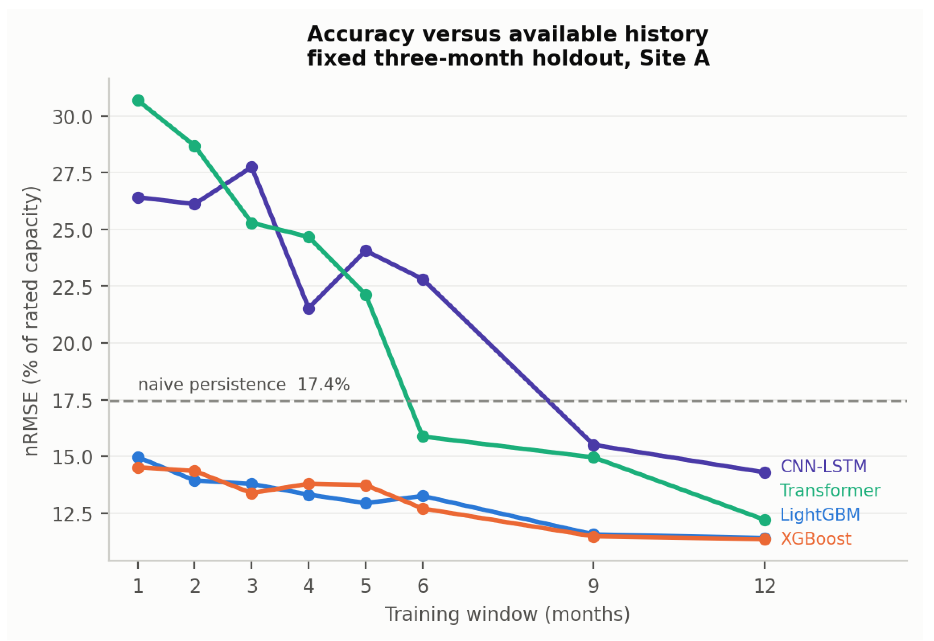
Figure 2.
XGBoost gain importance per feature (Site A). The one-hour lag and the short rolling window dominate; seasonal and calendar encodings that carry historic context are near zero.
Figure 2.
XGBoost gain importance per feature (Site A). The one-hour lag and the short rolling window dominate; seasonal and calendar encodings that carry historic context are near zero.
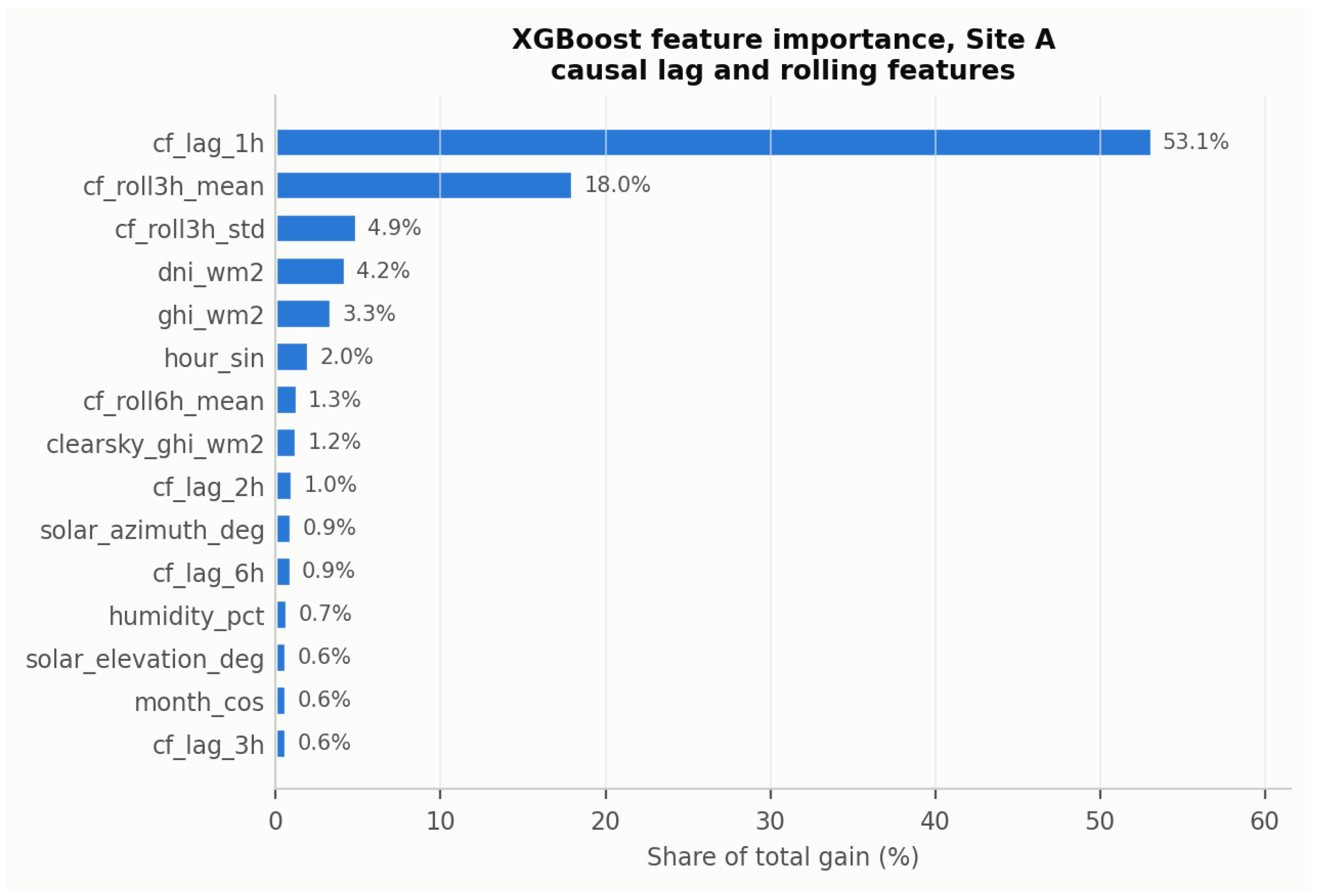
Figure 3.
Prospective May 2026 holdout (train January 2025–April 2026). Left: normalized RMSE; right: coefficient of determination. Gradient boosting leads on a month unseen during training, but by the smallest margin in the study.
Figure 3.
Prospective May 2026 holdout (train January 2025–April 2026). Left: normalized RMSE; right: coefficient of determination. Gradient boosting leads on a month unseen during training, but by the smallest margin in the study.
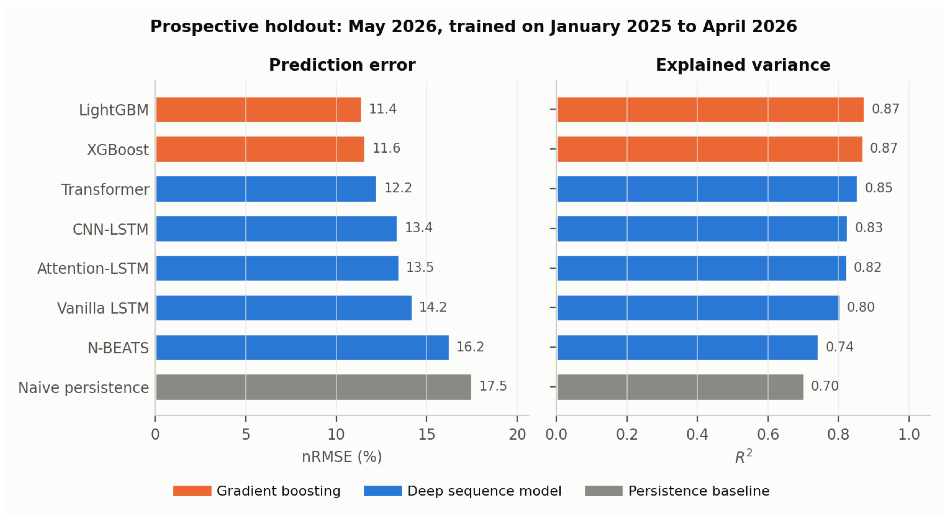
Figure 4.
Aligned per-model nRMSE at both sites. The ranking is preserved, and gradient boosting leads at each site.
Figure 4.
Aligned per-model nRMSE at both sites. The ranking is preserved, and gradient boosting leads at each site.
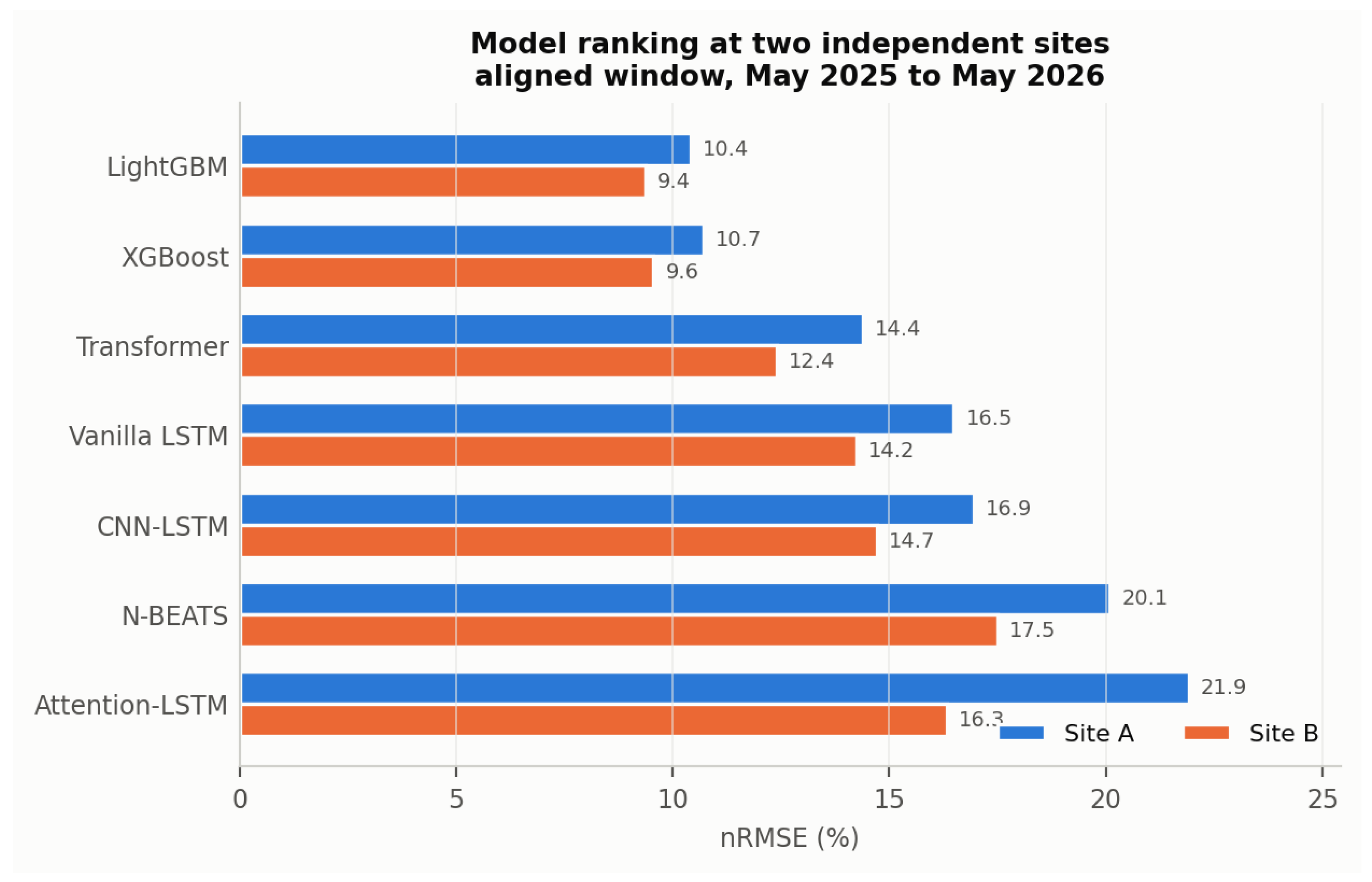
Figure 5.
Site A versus Site B model ranks. Points lie close to the diagonal (Spearman , ); the top five ranks are identical and only one adjacent pair swaps.
Figure 5.
Site A versus Site B model ranks. Points lie close to the diagonal (Spearman , ); the top five ranks are identical and only one adjacent pair swaps.
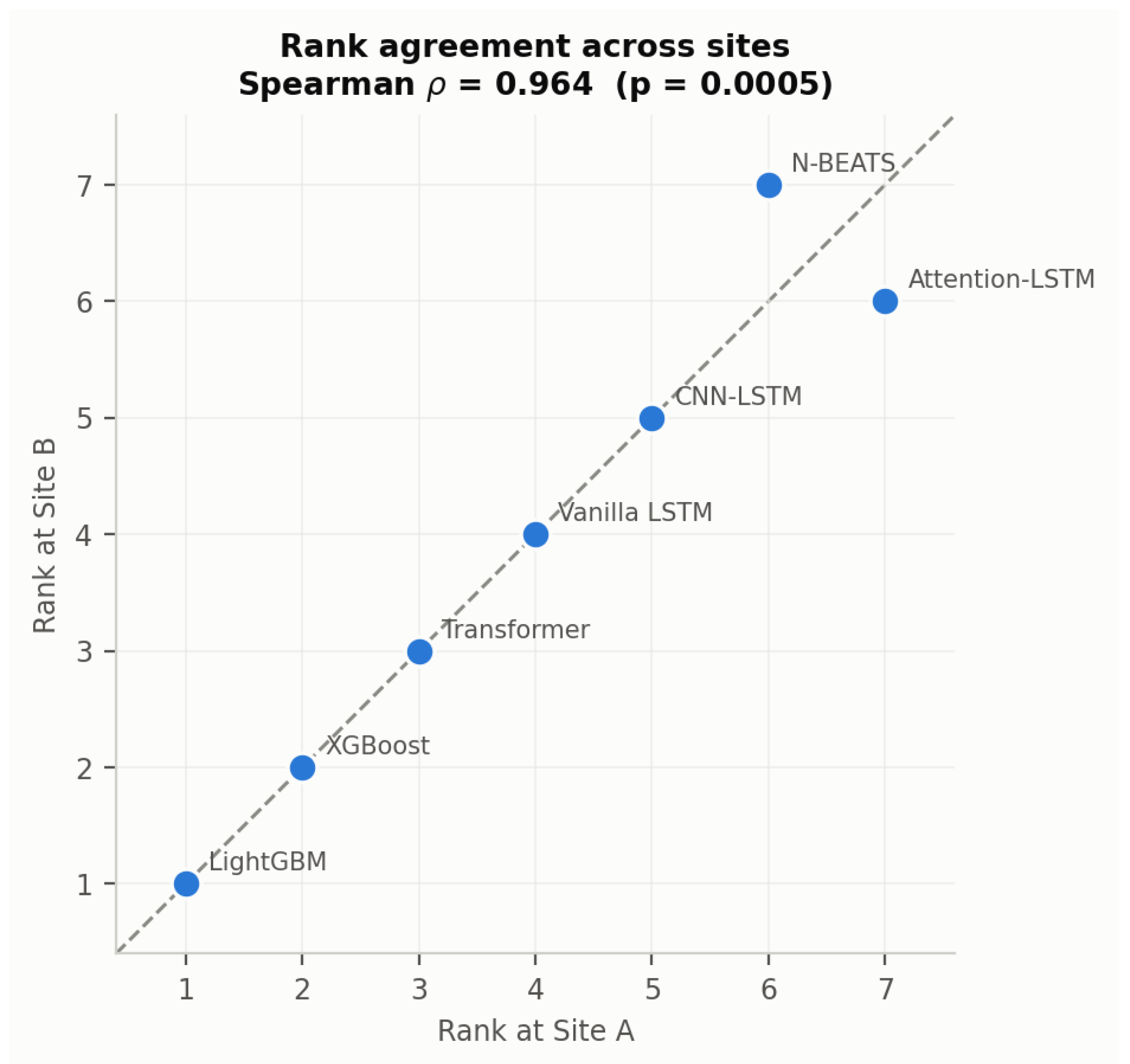
Figure 6.
Production XGBoost walk-forward at both sites: nRMSE for each successive test month over the site’s full history. Accuracy stays between 7% and 13% throughout and below naive persistence at both installations.
Figure 6.
Production XGBoost walk-forward at both sites: nRMSE for each successive test month over the site’s full history. Accuracy stays between 7% and 13% throughout and below naive persistence at both installations.
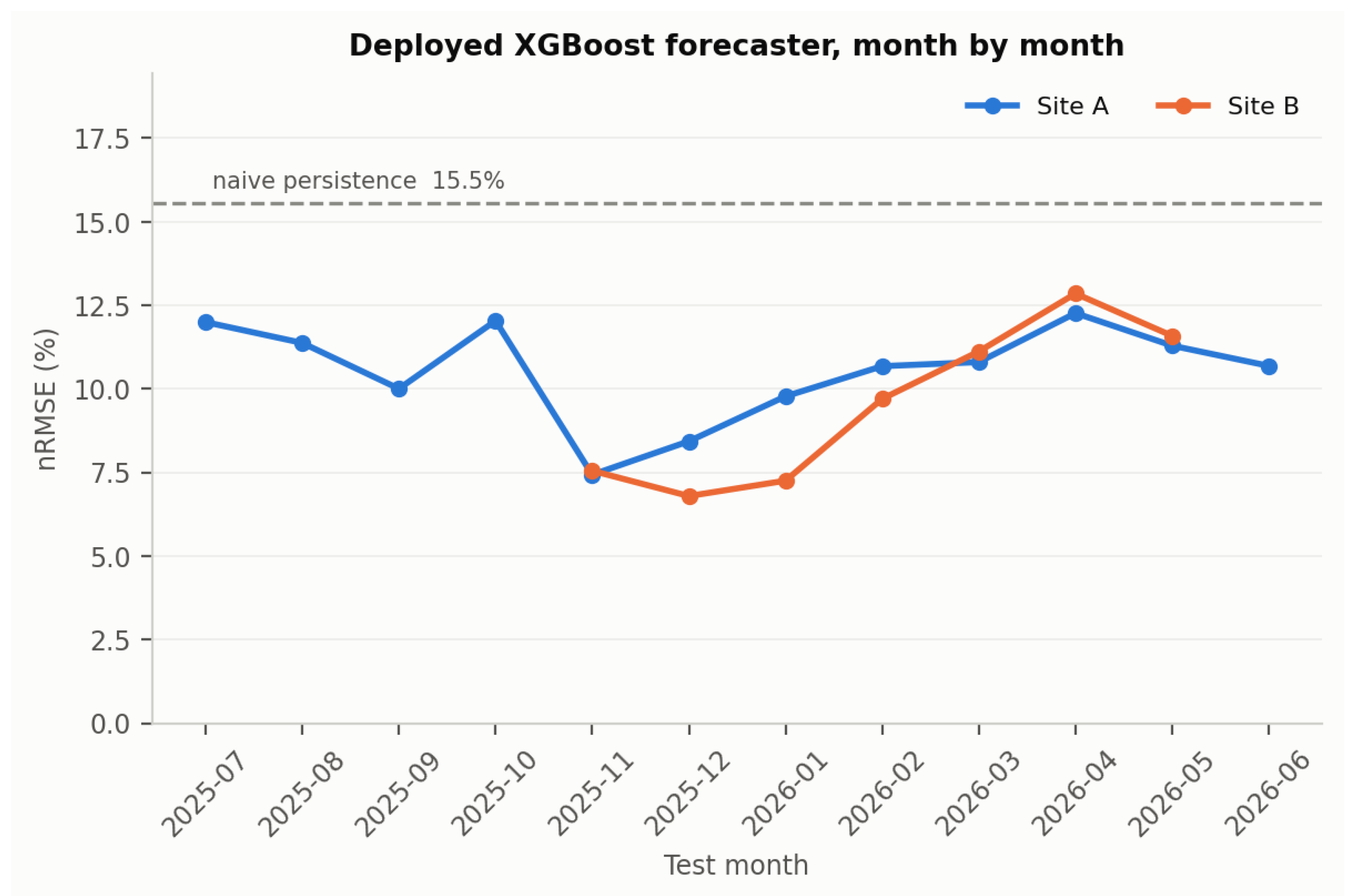
Figure 7.
Operational forecast of May–June 2026 at Site A. Top: daily energy, recorded against forecast, with the boundary of the known-weather window marked. Bottom: hourly nRMSE by horizon week against a climatology-only reference; error tracks the weather regime rather than distance from the origin.
Figure 7.
Operational forecast of May–June 2026 at Site A. Top: daily energy, recorded against forecast, with the boundary of the known-weather window marked. Bottom: hourly nRMSE by horizon week against a climatology-only reference; error tracks the weather regime rather than distance from the origin.
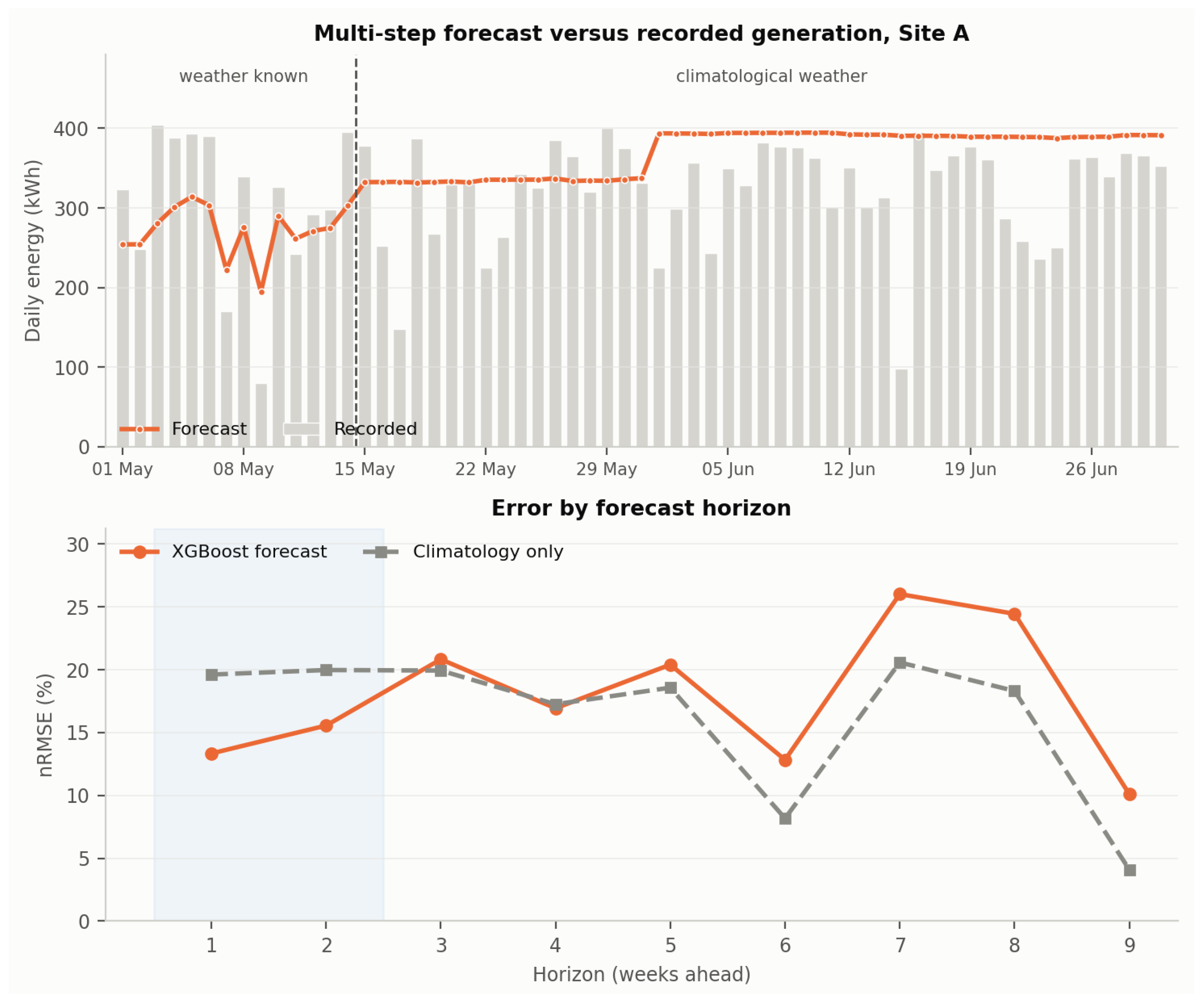
Figure 8.
Forecast error against the lead time of the weather input, Site A, May–June 2026. A day-ahead forecast costs 0.4 points relative to perfect weather; by seven days the weather-driven forecast is indistinguishable from one that uses no weather at all.
Figure 8.
Forecast error against the lead time of the weather input, Site A, May–June 2026. A day-ahead forecast costs 0.4 points relative to perfect weather; by seven days the weather-driven forecast is indistinguishable from one that uses no weather at all.
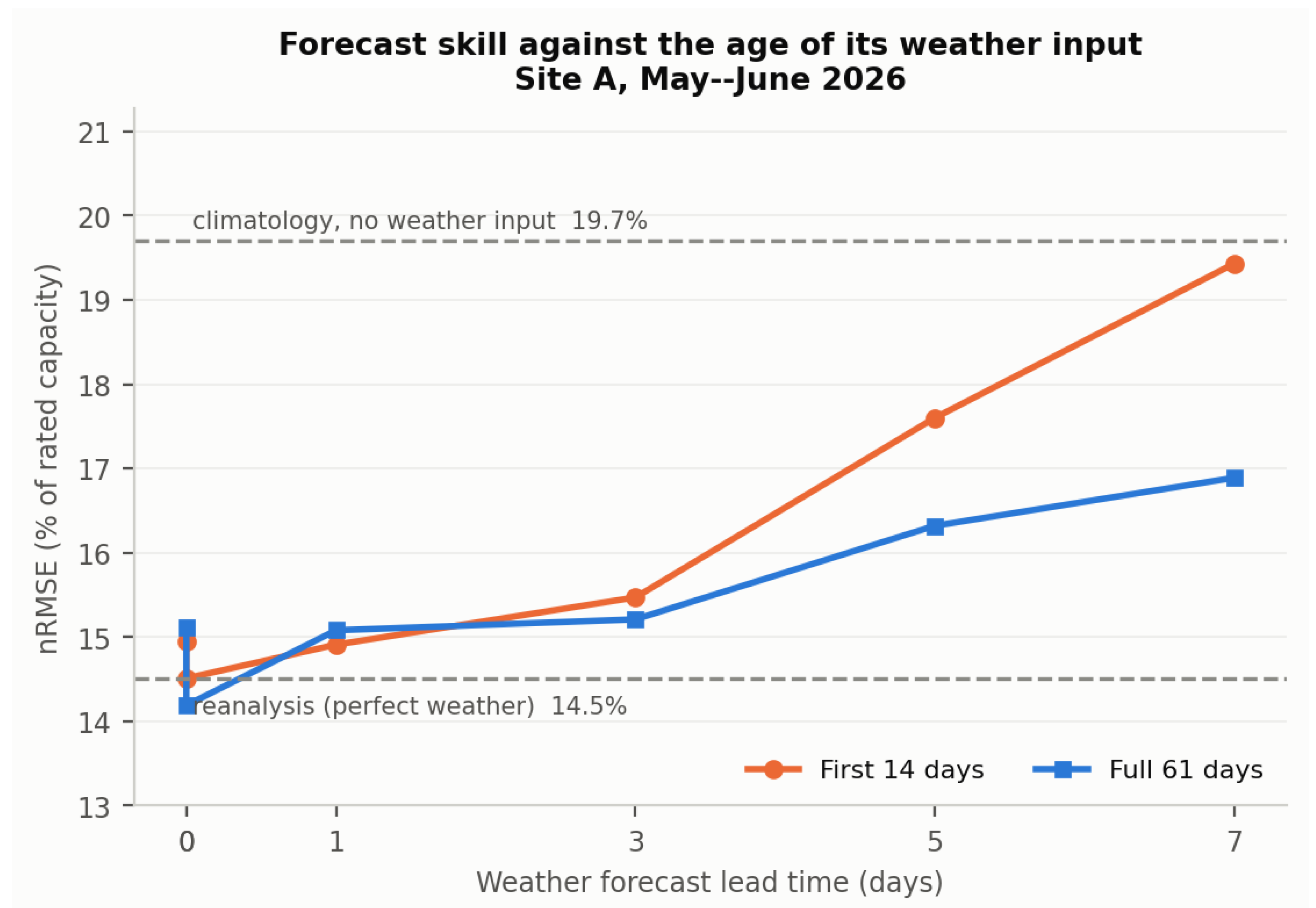
Figure 9.
Recency correction across 19 forecast origins at both sites. Top: the estimated multiplicative factor, which departs from 1.0 almost everywhere and saturates at the clip floor through winter. Bottom: its effect on forecast error, positive where the correction makes the forecast worse. The correction helps at 6 of 19 origins.
Figure 9.
Recency correction across 19 forecast origins at both sites. Top: the estimated multiplicative factor, which departs from 1.0 almost everywhere and saturates at the clip floor through winter. Bottom: its effect on forecast error, positive where the correction makes the forecast worse. The correction helps at 6 of 19 origins.
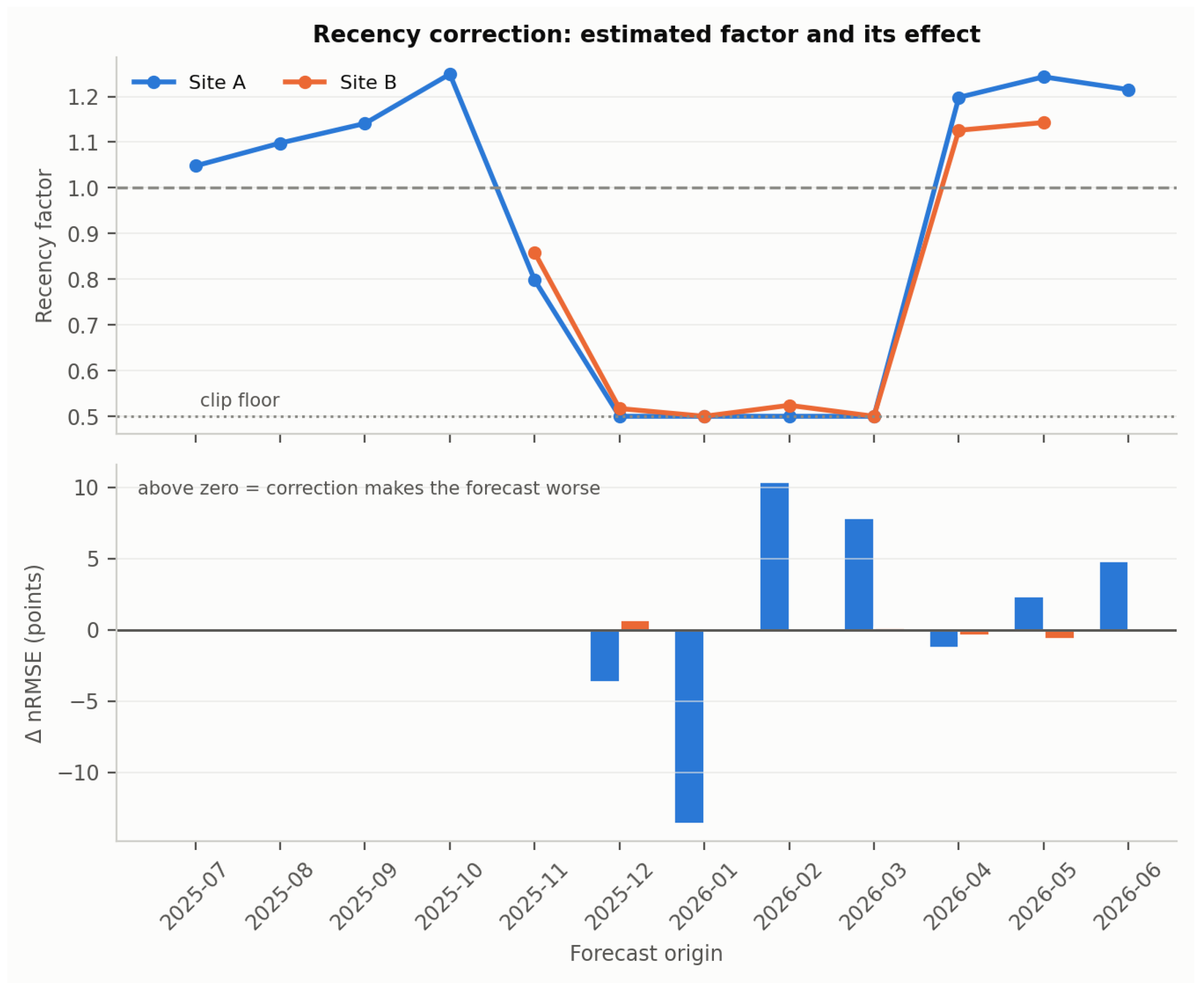
Table 1.
Model configurations and the hyperparameter grid searched on the temporal validation split (train: first five months of Site A; validate: the sixth). The Used column gives the single configuration held constant across every reported experiment.
Table 1.
Model configurations and the hyperparameter grid searched on the temporal validation split (train: first five months of Site A; validate: the sixth). The Used column gives the single configuration held constant across every reported experiment.
| Model | Architecture | Used | Searched |
|---|---|---|---|
| XGBoost | Depth-wise boosted trees | 500 trees, depth 6, lr 0.05, row/col subsample 0.8, min child weight 3 | trees , depth , lr |
| LightGBM | Leaf-wise boosted trees | 500 trees, depth 6, lr 0.05, row/col subsample 0.8, min 20 samples/leaf | as XGBoost |
| Vanilla LSTM | Single recurrent layer | 64 hidden units, dropout 0.2, linear read-out | hidden width |
| CNN-LSTM | 1-D convolution then LSTM | 64 filters, kernel 3, max-pooling; 64-unit LSTM | hidden width |
| Attention-LSTM | LSTM with additive attention | 64 units, Bahdanau attention over hidden states | hidden width |
| Transformer | Self-attention encoder | , 2 heads, 128-unit feed-forward, dropout 0.1 | hidden width |
| N-BEATS | Basis expansion | 2 stacks × 3 generic blocks, 4-layer MLP of 128 units | hidden width |
Table 4.
nRMSE versus training-window size on a fixed three-month holdout (Site A). Naive persistence on the same holdout scores 17.43%.
Table 4.
nRMSE versus training-window size on a fixed three-month holdout (Site A). Naive persistence on the same holdout scores 17.43%.
| Model | 1 mo | 3 mo | 6 mo | 9 mo | 12 mo |
|---|---|---|---|---|---|
| XGBoost | 14.52% | 13.38% | 12.70% | 11.48% | 11.35% |
| LightGBM | 14.97% | 13.79% | 13.26% | 11.56% | 11.40% |
| Transformer | 30.69% | 25.29% | 15.88% | 14.96% | 12.21% |
| CNN-LSTM | 26.42% | 27.74% | 22.81% | 15.51% | 14.29% |
Table 5.
XGBoost feature-group ablation on Site A. nRMSE is the change when the group is removed; larger positive values mean the group is more important.
Table 5.
XGBoost feature-group ablation on Site A. nRMSE is the change when the group is removed; larger positive values mean the group is more important.
| Ablated Group | nRMSE | nRMSE | Impact |
|---|---|---|---|
| Lag features (4) | 11.66% | Moderate | |
| Rolling statistics (3) | 10.70% | Low | |
| Weather (7) | 10.70% | Low | |
| Solar geometry (5) | 10.57% | Negligible | |
| Time encodings (6) | 10.52% | Negligible | |
| Baseline (28) | 10.51% | 0.00 | — |
| Physics-derived (3) | 10.45% | Negative |
Table 6.
Effect of adding three physics-informed features (25 vs 28 features) on Site A nRMSE. is 28-feature minus 25-feature.
Table 6.
Effect of adding three physics-informed features (25 vs 28 features) on Site A nRMSE. is 28-feature minus 25-feature.
| Model | 25 feat. | 28 feat. | |
|---|---|---|---|
| XGBoost | 10.64% | 10.59% | |
| LightGBM | 10.45% | 10.39% | |
| Transformer | 13.56% | 12.88% | |
| CNN-LSTM | 15.92% | 15.43% |
Table 7.
Retraining strategy on Site A (walk-forward, 12 iterations).
| Configuration | nRMSE | MAE (kW) | |
|---|---|---|---|
| LightGBM scratch | 10.39% | 3.38 | 0.875 |
| XGBoost scratch | 10.51% | 3.46 | 0.872 |
| LightGBM warm-start | 10.91% | 3.61 | 0.862 |
| XGBoost warm-start | 11.11% | 3.67 | 0.857 |
| Transformer warm-start | 12.54% | 4.29 | 0.816 |
| Transformer scratch | 13.25% | 4.60 | 0.789 |
Table 8.
Ensemble strategies on Site A. Members: XGBoost, LightGBM, warm-start Transformer.
| Configuration | nRMSE | MAE (kW) | |
|---|---|---|---|
| Stacking (ridge) | 10.35% | 3.39 | 0.875 |
| LightGBM solo | 10.39% | 3.38 | 0.875 |
| XGBoost solo | 10.51% | 3.46 | 0.872 |
| Weighted average | 10.53% | 3.48 | 0.871 |
| Simple average | 10.62% | 3.52 | 0.869 |
| Transformer (warm-start) | 13.03% | 4.40 | 0.799 |
Table 9.
Aligned dual-site comparison (nRMSE) over the identical May 2025–May 2026 window.
| Rank | Model | Site A (Aligned) | Site B |
|---|---|---|---|
| 1 | LightGBM | 10.41% | 9.37% |
| 2 | XGBoost | 10.70% | 9.55% |
| 3 | Transformer | 14.38% | 12.40% |
| 4 | Vanilla LSTM | 16.49% | 14.24% |
| 5 | CNN-LSTM | 16.95% | 14.71% |
| 6 | N-BEATS | 20.09% | 17.49% |
| 7 | Attention-LSTM | 21.91% | 16.33% |
Table 10.
Multi-step forecast of May–June 2026 at Site A, trained on January 2025–April 2026, with no observation from the forecast period. Hourly nRMSE over daytime hours.
Table 10.
Multi-step forecast of May–June 2026 at Site A, trained on January 2025–April 2026, with no observation from the forecast period. Hourly nRMSE over daytime hours.
| Segment | Forecaster | Climatology only | Gain |
|---|---|---|---|
| Days 1–14 (weather known) | 14.51% | 18.95% | |
| Days 15–61 (climatological) | 16.43% | 16.72% | |
| Full 61-day horizon | 16.02% | — | — |
Table 11.
Forecast accuracy by the age of the weather input (Site A, May–June 2026, no observation from the horizon). GHI error is the RMSE of the input’s global horizontal irradiance against the reanalysis over daytime hours.
Table 11.
Forecast accuracy by the age of the weather input (Site A, May–June 2026, no observation from the horizon). GHI error is the RMSE of the input’s global horizontal irradiance against the reanalysis over daytime hours.
| Weather input | Days 1–14 | Full 61 days | GHI error (W/m2) |
|---|---|---|---|
| Reanalysis (perfect) | 14.51% | 14.19% | 0 |
| Analysis (lead 0) | 14.95% | 15.11% | 80 |
| Forecast, lead 1 day | 14.91% | 15.08% | 96 |
| Forecast, lead 3 days | 15.47% | 15.21% | 99 |
| Forecast, lead 5 days | 17.60% | 16.32% | 142 |
| Forecast, lead 7 days | 19.43% | 16.89% | 138 |
| Climatology (no weather input) | 19.70% | 17.23% | — |
Disclaimer/Publisher’s Note: The statements, opinions and data contained in all publications are solely those of the individual author(s) and contributor(s) and not of MDPI and/or the editor(s). MDPI and/or the editor(s) disclaim responsibility for any injury to people or property resulting from any ideas, methods, instructions or products referred to in the content. |
© 2026 by the authors. Licensee MDPI, Basel, Switzerland. This article is an open access article distributed under the terms and conditions of the Creative Commons Attribution (CC BY) license (http://creativecommons.org/licenses/by/4.0/).
Copyright: This open access article is published under a Creative Commons CC BY 4.0 license, which permit the free download, distribution, and reuse, provided that the author and preprint are cited in any reuse.