

Submitted:
06 October 2026
Posted:
09 October 2026
Read the latest preprint version here
Abstract
The Spiral Structure Model (SSM) is a phenomenological model in the tradition of Bohr’s early atom: confined to kinematics and geometry, it exchanges dynamical depth for ontological clarity and experimental exposure. Three postulates suffice. (I) The photon is a pointlike energy quantum in uniform helical motion, its axial and circulation speeds both equal to c; (II) physical space is an elastic, relativistically covariant medium sustaining vortex excitations; (III) the electron is a stable topological vortex defect of that medium. From these — with every step carrying an explicit epistemic label — the model obtains the photon’s circulation angular momentum mcrγ = ℏ as a consistency theorem, identified with its spin; logarithmic vortex confinement with no free parameters; the two polarization states and the absence of a longitudinal mode; orbital angular momentum as an ensemble property; the electron’s 720-degree periodicity and spin ℏ/2 from π1(SO(3)) = Z2; the fine-structure constant as a ratio of structural scales; the free radiation field as a retarded ensemble moment satisfying the wave equation exactly; a phase-coupling account of two-slit interference; and a double-helix ontology of entangled pairs that reproduces the CHSH value 2√2. Three falsifiable discriminants are stated with explicit kill criteria: a wavelength-locked on-axis void in the photon’s detection profile, a spin-dependent electron form-factor window near Q = mc, and a circulation-periodic component in entangled-pair coincidence timing.
Keywords:
wave-particle duality
; photon structure
; electron spin
; fine-structure constant
; Bell correlations
; phenomenological model
; quantum foundations
1. Introduction
1.1. The Interpretive Deficit of Quantum Mechanics
Quantum mechanics is operationally complete and ontologically opaque. Its formalism predicts measurement statistics with unrivaled precision, yet it declines to say what a photon [1] or an electron is between preparation and detection. The Copenhagen tradition elevated this reticence into a principle. The de Broglie–Bohm tradition answered it with trajectories guided by a wave [2,3], a program developed to maturity in the ontological interpretation of Bohm and Hiley [4]. Schrödinger’s zitterbewegung [5] and Dirac’s spinor equation [6] showed that internal motion at light speed and a multi-component structure are already latent in the relativistic formalism itself. The EPR argument [7] and Bell’s theorem [8] then fixed the terms of any realist completion: the quantum objects, whatever they are, cannot be simultaneously local and possessed of definite pre-existing properties in the naive sense. More recently, the Pusey–Barrett–Rudolph theorem [9] has sharpened the ontological question further: under mild assumptions, the quantum state itself must be physically real rather than a mere summary of information about the system.
The Spiral Structure Model (SSM) belongs to the geometric-realist lineage of de Broglie’s theory of the double solution [2]. Its kinematic core is the hypothesis, originally Einstein’s [1], that the photon is a genuine quantum of energy; the model asks what geometric form such a quantum must have if its spin, its polarization, and its wave-like statistics are to be properties of the object itself rather than of a probability field attached to it. A companion natural-philosophical account of the same framework, with the full deductive apparatus from axioms to experimental schemes, has been given elsewhere [10]; the present paper is the phenomenological core of that program, presented for judgment by the standards of theoretical physics.
1.2. The Phenomenological Stance
The model is offered as a phenomenological one, and we ask that it be judged by the standards of that genre rather than by those of a fundamental theory. The genre has a distinguished pedigree. Bohr’s atomic model [11] reproduced the Rydberg constant from a single quantization postulate while contradicting the electrodynamics of its day, and it organized spectroscopy for a decade before its successor existed. The Ginzburg–Landau theory [12] classified the electrodynamics of superconductors years before any microscopic derivation was available, and it remains a working tool of that field. Such models share a profile: few geometric assumptions, a unifying picture, semi-quantitative success, sharp predictions, and an openly acknowledged dynamical deficit. They are judged by fertility, coherence, and risk, not by rigor.
Two contemporary research programs mark the coordinates within which the SSM should be located. The axiomatic reconstructions of quantum theory in the spirit of Hardy [13] share the ambition of accounting for the formalism from a few principles, but remain deliberately agnostic about what the quantum objects are. Deterministic completions such as ’t Hooft’s cellular automaton interpretation [14] share the ontological ambition, but differ from the present model both in mechanism and in what they take to be fundamental. The SSM sits between these poles: ontologically committal like the second, and modest in its mathematical machinery like the first. Three further programs that share the SSM’s territory — hydrodynamic quantum analogs, stochastic and emergent reconstructions of quantum statistics, and the photon wave-function debate together with its weak-measurement experiments — are confronted explicitly in Section 1.3.
The SSM is built to this profile. It is restricted, deliberately, to kinematics and geometry; the dynamics of the medium is postponed and recorded as an open problem rather than smuggled in through notation. Within that restriction it unifies phenomena usually kept apart: interference, spin, the absence of longitudinal photons, the strength of Bell correlations, the scale of the electromagnetic coupling, and the free-space wave equation all follow from one geometric object and its ensemble statistics. In return the model accepts the discipline of the genre: three of its predictions are stated with protocols and kill criteria (Section 8), and every component that fails its own criteria is replaced in full view rather than concealed (Section 2.1, Section 3.1, Section 3.2, Section 3.5 and Section 6).
1.3. Neighboring Research Programs: What the SSM Must Answer To
Three contemporary research programs occupy the territory closest to the SSM, and placing the model requires confronting each of them directly. First, the hydrodynamic quantum analogs: silicon-oil droplets bouncing on a vibrating bath reproduce single-particle diffraction and interference [33], tunneling, quantized orbits, and Fraunhofer-like statistics through a macroscopic pilot-wave dynamics of finite memory [34]. The analogy is genuine but bounded: the droplet’s wave is a physical surface wave coextensive with the particle, whereas in the SSM the individual quantum is the helical object and the wave is an ensemble shadow (Section 3.4 and Section 3.5). The SSM shares the analogs’ ontological clarity and borrows their empirical lesson — that statistical, wave-like behavior need not imply intrinsic randomness — without claiming their mechanism.
Second, stochastic electrodynamics and classical-statistical reconstructions of quantum statistics [35,36] derive large parts of the formalism from a real stochastic background. The SSM differs on the decisive point: its randomness is not dynamical noise but the uniform distribution of a geometric entry coordinate (the circulation phase), so the model retains determinism at the single-event level while reproducing quantum statistics at the ensemble level. Third, the photon wave-function debate [37,38,39] shows that no position-space probability amplitude exists for a single photon, while weak-measurement experiments have demonstrated that average photon trajectories [23] and even an operational photon wavefunction [40] can be measured directly. This is precisely the semantic niche the SSM occupies: its ensemble constructions are statements about measurable averages of real circulations, not about a single-photon wavefunction the formalism forbids.
For the electron, the SSM stands in the line of classical and relativistic models of spin as circulation energy flux: Ohanian’s demonstration that spin is a circulating momentum density of the Dirac field [41], the velocity-field models of Salesi and Recami [42], the zitterbewegung geometry of Barut and Bracken [43], and Hestenes’ reading of the Dirac theory [24]. The S-motion of Section 4 adds one element these predecessors lack: the 720° periodicity is not an additional hypothesis but the homotopy class the defect must realize (Equation (11)). Finally, the medium postulate (Section 2.5) must be read against the strongest modern aether-drift bounds, obtained with continuously rotating and cryogenic optical resonators, which constrain any anisotropy of c to the 10−17 level [44,45]; the SSM’s reply is the emergent-invariance mechanism of Section 2.6, and we record the residual tension as open problem 2 rather than as resolved.
1.4. Method: Axiomatization with Epistemic Stratification
The construction follows the axiomatic spirit of Hilbert’s sixth problem: isolate a minimal set of geometric postulates, derive what follows rigorously, and mark the points where empirical input, modeling choice, or guesswork enters. Every statement in this paper therefore carries an explicit epistemic label. We distinguish Postulates (free hypotheses, judged by fruitfulness), Theorems (rigorous consequences of stated premises, possibly conditional on empirical inputs), Identities (algebraic restatements with interpretive but no predictive content), Models (concrete mechanisms with adjustable coefficients), and Predictions (statements exposed to experimental disproof). A framework that knows the logical status of its own parts can be criticized and improved component by component instead of being accepted or rejected as a monolith.
Two historical failures motivate this discipline. Hidden-variable models were long dismissed wholesale because individual poorly framed instances failed; stratification allows the sound parts of such a model to survive the unsound ones. And realist models have repeatedly oversold algebraic coincidences as derivations. An example appears in Section 2.2, where the relation mcrγ = ℏ proves to be a consistency theorem rather than an independent derivation, and is labeled accordingly.
1.5. Scope, and What We Do Not Claim
The SSM does not compete with quantum electrodynamics in precision, and nothing in this paper should be read as a claim to reproduce the eight-decimal successes of the anomalous magnetic moment. The framework aims at a different target: a single geometric ontology from which the qualitative architecture of the quantum follows as properties of objects in space and time. Where a component of the framework fails its own criteria, the failure is stated and the component replaced (Section 2.1, Section 3.1, Section 3.2, Section 3.5 and Section 6). Where the model is vulnerable to experiment (Section 8), the vulnerability is stated as explicit falsification conditions (Section 9.3).
One bridge obligation follows from this choice of scope and is stated now rather than later: the completed dynamics must recover the Schrödinger and Dirac equations, and with them the Hilbert-space description, as effective structures of the medium. We regard this recovery as a condition on any acceptable completion of the model, and it is recorded among the open problems (Section 9.2).
The corresponding objection — that a model confined to kinematics cannot compute processes and therefore is not physics — deserves a direct answer. Bohr’s 1913 model supplied no dynamics for its stationary states either; what it supplied was constraint, unification, and risky contact with spectroscopy, and it organized a decade of experimental work before its dynamical successor existed. A phenomenological model is properly judged by four obligations: internal consistency, unification of previously separate phenomena, falsifiable contact with data, and an explicit statement of what the completed theory must recover. The present framework discharges all four, and claims nothing beyond them. Nor are the framework’s consistency theorems idle restatements: each one fixes a structure — the circulation radius, the two helicities, the absence of a longitudinal mode — that a later section converts into a discriminating prediction. The genre’s historical successes were built from exactly such conversions.
2. The Three Postulates
2.1. Postulate I: The Photon as a Helical Quantum
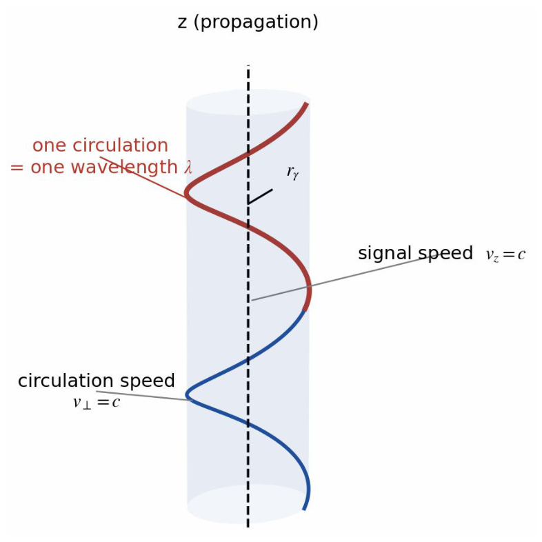
Postulate I [P]. A photon of energy E is a pointlike energy quantum of inertial mass m = E/c2 whose center of energy executes uniform helical motion. In a frame in which the photon propagates along the z-axis, the trajectory image is
r(t) = (rγ cos ωt, rγ sin ωt, ct) (1)
where rγ is the circulation radius and ω the circulation frequency. Two speeds are fixed by the postulate: the axial speed vz = c, the signal velocity of the quantum, and the circulation speed v⊥ = ωrγ = c, the internal motion of an excitation that possesses no rest frame.
Status statement [P, phenomenological kinematics]. The helix of Equation (1) is a kinematic image of the quantum’s energy transport, not a worldline in the Minkowski sense: its Euclidean arc-rate is √2 c, and no curve traced by a material point in spacetime — timelike or null — has that property. The model therefore makes no claim about the spacetime classification of the trajectory, and it needs none. What it claims is that the observable kinematics of the photon is exhausted by quantities that respect special relativity exactly: a signal velocity c along the axis, a translational momentum p = mc directed along the axis, and the energy–momentum relation E = pc, which involves the signal velocity alone. The circulation carries angular momentum but no translational energy, exactly as the rim motion of a spinning body contributes rotational but not translational kinetic accounting. The three conceptually distinct speeds of the model, and their distinct physical roles, are collected in Table 1. The arc-rate √2 c is a property of the curve, not a signal speed: it parametrizes a geometric image, and nothing physical propagates along the wire of the helix. The spacetime interpretation of the helix itself belongs to the medium theory (open problem 2). The separation between the instantaneous speed of an internal motion and the observable signal speed has a precedent within standard theory itself: in the Dirac equation the velocity operator has eigenvalues ±c although no observed motion attains c, and the zitterbewegung reading of the Dirac theory [24] exploits precisely this gap between geometric and observable kinematics.
Figure 1.
The trajectory image of Postulate I. The pointlike quantum circulates at radius rγ = λ/(2π) around the propagation axis with circulation speed v⊥ = c while the axis advances at the signal speed vz = c; one circulation is completed per axial advance of one wavelength λ. The geometric arc-rate √2 c is a property of the curve, not a signal speed (Table 1).
Bookkeeping note. The particle-language expression L = m v⊥rγ used below is the heuristic wrapper of a classical wave identity: circularly polarized radiation carries angular momentum per unit energy L/E = 1/ω, established by Beth’s mechanical measurement [15]. With ω = c/rγ the two forms coincide, mcrγ = E/ω. The wave form is primary; it requires no notion of photon rest mass, and the helicity it describes is a Lorentz-invariant property of a massless excitation.
2.2. The Relation Mcrγ = ℏ as a Conditional Consistency Theorem
From Postulate I, one circulation is completed while the axis advances by one wavelength:
2πrγ = cT = c/ν ⟹ ν = c/(2πrγ) (2)
Combining with the two empirical pillars of the quantum, E = hν (Planck–Einstein) and E = mc2 (relativity), yields
mc2 = hν = hc/(2πrγ) ⟹ mcrγ = ℏ (3)
Theorem 1 (consistency, not derivation) [T, conditional]. Given Postulate I and the two empirical relations above, the circulation angular momentum of the photon about its axis equals ℏ. Epistemic note. We state what Equation (3) is and what it is not. It is not an independent derivation of a new formula: the chain ν → E = hν → E = mc2 → mcrγ = ℏ uses both quantum postulates as inputs, so the output can contain no information they did not already possess. A critic who calls the argument circular is right about its logical form. What Equation (3) establishes is a consistency theorem: the two historically independent formulas E = hν and E = mc2 are exactly the azimuthal and axial faces of a single geometric object, and the helix supplies the bridge that the point-particle ontology lacks. The value of the theorem is unification and constraint: the circulation radius is fixed, not free, The theorem thereby earns its keep as a generator rather than as an explanation: it converts two known relations into a definite spatial structure — a circulation radius fixed at the reduced wavelength — and it is that structure, not the algebra, which Section 3.2 and Section 8.1 convert into an experiment.
rγ = ℏ/(mc) = λ/(2π) (the reduced wavelength) (4)
so the photon’s transverse circulation scale is locked to its reduced wavelength. This lock is the source of the model’s first falsifiable discriminant (Section 8.1).
2.3. Postulate II: The Elastic Space Medium
Postulate II [P]. Physical space is an elastic, relativistically covariant medium that sustains and guides vortex excitations; all disturbance speeds in the medium are bounded by c. The postulate supplies the restoring dynamics that stabilizes the photon circulation (Section 3.1) and the electron defect (Postulate III). One constraint is immediate. A classical elastic medium supports longitudinal as well as transverse excitations, whereas the free photon exhibits only two transverse polarization states (Section 3.2). The medium must therefore be effectively incompressible, or its longitudinal sector must be unphysical in the way gauge redundancy makes it unphysical in electrodynamics; identifying the mechanism is assigned to open problem 2. Status. This is the least constrained of the three postulates. It is stated at the level of physical intuition, and a constitutive theory with quantified constants is listed among the open problems (Section 9.2). The framework uses Postulate II only where it does real work, and every such use is labeled [M].
2.4. Postulate III: The Electron as a Topological Vortex Defect
Postulate III [P]. The electron is a stable topological defect (a vortex soliton) of the medium, with a geometric radius of the order of the reduced Compton wavelength, re ≡ ℏ/(mc) = 3.862 × 10⁻¹³ m. The vortex topology supplies the stability that a classical extended charge distribution lacks.
Definition 1 (two radii) [essential conceptual separation]. We distinguish throughout: (i) the geometric radius re, the extent of the vortical flow pattern in the medium; and (ii) the charge radius rcharge, the region in which the electromagnetic charge density is concentrated. High-energy scattering and the electron g − 2 constrain rcharge≲10−18 m; they say nothing about re, because the vortical flow carries negligible charge density beyond the core. The apparent conflict between a finite geometric structure and the pointlike electrodynamic tests is thereby removed at the level of definitions [T, given the distinction].
2.5. Lorentz Covariance: Postulated, Not Derived, and the Empirical Envelope
Status statement [P, with open derivation]. Postulate II asserts that the medium is relativistically covariant; it does not derive covariance. This is the classical difficulty of every medium-based ontology: an elastic medium appears to single out a preferred rest frame, and the burden is on the model to show how an effectively Lorentz-invariant dynamics of excitations emerges, in the way that acoustic excitations of a condensed-matter system obey an effective relativistic wave equation even though the underlying lattice prefers a frame [16]. The SSM does not yet discharge this burden; the emergence proof is part of open problem 2. What can and must be done at this stage is to state the empirical envelope inside which any such dynamics must live.
Empirical envelope [experimental constraints the model must respect]. Michelson–Morley-type experiments, in their modern optical-resonator descendants, bound an anisotropy of the speed of light at Δc/c ≲ 10−17; Kennedy–Thorndike-type tests bound the boost dependence of c at ≲ 10−8; Ives–Stilwell-type measurements confirm relativistic time dilation and bound the corresponding test-theory parameter at ≲ 10−8; and the photon-sector coefficients of the Standard-Model Extension are bounded at the 10−16 to 10−18 level [17,18]. The consequence for the SSM is direct: the medium’s excitations must reproduce special relativity to these precisions, and any Lorentz-violating relic of the medium’s rest frame must hide below them. Should the completed field theory predict a relic above these bounds, Postulate II is falsified in its present form (Section 9.3).
2.6. A Mathematical Pathway for the Medium
A concrete template [M]. The program of Postulate II has a known mathematical shape. A relativistic medium that selects a preferred foliation while preserving local Lorentz invariance for all excitations is realized, in the gravitational context, by Einstein–aether theory: a unit timelike vector field ua coupled covariantly to a metric, whose excitation spectrum contains precisely the longitudinal and transverse modes that an elastic medium suggests [19]. The SSM medium is the non-gravitational analogue of that construction: a covariant elastic continuum whose rest frame is observationally hidden because all universal disturbance speeds equal c. The incompressibility constraint of Section 2.3 translates, in that language, into a condition on the longitudinal sector.
Emergence precedent [M]. That an elastic medium can generate effectively Lorentz-invariant dynamics for its excitations is not a hope but a precedent: in superfluid 3He the collective coordinates obey relativistic wave equations and experience an effective metric, while the underlying atoms select a frame [16]. The SSM claims no more than the same logical possibility for physical space. What remains open — open problem 2 — is the specific action whose vortex sector yields the logarithmic self-energy of Section 3.1 and whose defect sector yields Postulate III.
3. The Photon: Confinement, Helicity, and the Ensemble Origin of the Wave
3.1. The Self-Induced Vortex Potential: Failure of the Power Law, and the Logarithmic Form
The power-law ansatz, excluded. A natural first choice for the self-induced attraction is a power law, Uind(r) = −mc2rγ2/(2r2), with the coefficient fixed by requiring equilibrium at r = rγ. It fails for cause. With angular momentum conserved, the induced term cancels the centrifugal barrier ℏ2/(2mr2) identically at every radius: the effective potential is flat, and r = rγ is a neutral equilibrium with no restoring force. With the tangential speed instead constrained to c (Postulate I), the radial force balance makes r = rγ an unstable equilibrium: a quantum displaced outward is accelerated further outward, and one displaced inward collapses. In neither reading does the power law deliver the stable bound configuration the framework requires, and it is excluded.
Model construction [M]: the logarithmic vortex self-energy. The physical picture of Postulate II points to a different functional form. In two dimensions the functional form is not a choice but a constraint: an incompressible, irrotational flow in the annulus around the core obeys ∇·u = 0 and ∇×u = 0, whose unique scale-free solution is uθ(ρ) = Γ/(2πρ), and the kinetic energy stored in that flow per unit length is therefore logarithmic, ∝ Γ2 ln(ρ/rγ) — the standard result of vortex energetics. Any self-induced confinement of a circulation quantum in two dimensions has this functional form; the only freedom is the coefficient. Displacing the quantum from its circulating orbit therefore costs a logarithmically growing self-energy, and the effective radial potential for the circulation quantum ℏ is
Ueff(ρ) = ℏ2/(2mρ2) + A ln(ρ/rγ) (5)
where the first term is the centrifugal barrier of the unit circulation and the second is the vortex self-energy. Equilibrium requires dUeff/dρ = 0, i.e., ρ2 = ℏ2/(mA). The coefficient is then over-determined in the model’s favor: with the circulation quantized at Γ = h/m (unit angular momentum per unit mass) and the radius locked to rγ = ℏ/(mc), the only energy constructible from m, c, and rγ is mc2, so dimensional analysis alone gives A ∼ mc2; requiring the minimum to coincide with the radius of Equation (4) fixes the remaining order-unity factor to one, with no free parameter:
A = ℏ2/(mrγ2) = mc2 ⟹ minimum at ρ = rγ (6)
The equilibrium is genuinely stable: the curvature U″eff(rγ) = 2mc2/rγ2 > 0, and small radial displacements oscillate at the breathing frequency ωrad = √(U″eff/m) = √2 c/rγ = √2 ω, above the circulation frequency. The result is a stable bound configuration of definite radius with zero adjustable coefficients (Figure 2). Status. The logarithmic form is a model potential motivated by two-dimensional vortex energetics, not the output of a fundamental field equation; deriving it from a covariant action for the medium is open problem 2 (Section 9.2).
3.2. The Two Helicities, the Absent Longitudinal Mode, and Orbital Angular Momentum as an Ensemble Property
Theorem 2 [T, within the model]. Requiring the circulation phase to be single-valued over each axial period (the quantum condition on the helix) selects the ground-state radius of Equation (4); combined with Theorem 2.1, the circulation angular momentum is
L = m v⊥rγ = ℏ, σ = ±1 (7)
and the two senses of circulation are the two helicity states of the photon. That a circularly polarized beam carries angular momentum ±ℏ per quantum is itself an experimental fact [15].
Identification [M, essential]. The circulation angular momentum of Equation (7) is identified with the spin angular momentum of the photon itself, and not with any orbital content: spin, in this framework, is the mechanical angular momentum of the quantum’s intrinsic circulation [10]. A longitudinal (m = 0) state would correspond to a helix of zero handedness — a straight line — which carries no circulation and hence no angular momentum; the model thereby supplies a geometric reason for the observed absence of the longitudinal polarization mode of the free photon [M].
Orbital angular momentum [M, ensemble-level]. The framework draws the corresponding line on the other side with equal explicitness: orbital angular momentum (OAM) is not a property of one quantum. A beam carrying a spiral phase wavefront eilθ [20] is, in this picture, a phase-synchronized collective winding of many quanta, each of which carries only its own circulation ℏ; the beam’s lℏ reflects the quantized head-count of coherently winding quanta rather than an intrinsic quantum number of a single photon. This stratification is consistent with the conservation bookkeeping of the OAM literature [20,21] and with the fact that OAM values are always reconstructed from ensemble statistics. What it does not yet explain is the deterministic single-event response of mode sorters to heralded quanta prepared in high-l states [21,22], where individual detection events are sorted with near-unit efficiency. We record this as open problem 10: the collective picture must either reproduce the single-event record or be amended, and we state the obligation rather than paper over it.
The on-axis void as kinematics [T, conditional on Postulate I]. Because the quantum circulates at ρ = rγ and never occupies the axis, the transverse distribution of detection events of the free quantum is ring-supported: every photon carries an intrinsic on-axis void of geometric diameter 2rγ = λ/π. No quantized transverse mode may underwrite this void: an e^{iθ} spatial phase winding is an orbital-angular-momentum structure, and attaching it to the single quantum would conflate the intrinsic circulation — its spin, on the identification above — with an orbital degree of freedom, contradicting the stratification established here. The void rests on Postulate I alone. This strengthens rather than weakens the discriminant of Section 8.1: the experiment tests the postulate directly.
3.3. Two-Slit Interference Without Collisions: Phase-Boundary Coupling
Model construction [M]. The most obvious coupling available to the model, a mechanical collision between the photon and the slit walls, is untenable: interference persists in wall-free arrangements (grating and light-pulse interferometers), and any dissipative contact would imprint a continuous spectral redistribution of the transmitted light that interference phenomenology does not show. The coupling must be geometric and non-dissipative. We model it as a spiral phase-boundary coupling. The circulation phase φ(t) = ωt is a real internal degree of freedom, and a slit of finite width samples the transverse phase structure of the helix, imprinting a geometric phase offset δφ that depends on the slit geometry relative to rγ but requires no momentum transfer. The total phase difference at the screen is Slits are not essential to the mechanism: any element that localizes the quantum transversely — a grating period, an aperture edge, or the coating of a beam splitter — imprints the same geometric offset. The construction thus covers wall-free interferometers such as the Mach–Zehnder, where the offsets enter at the beam-splitter surfaces rather than at slit walls.
ΔΦ = (2π/λ)(L2 − L1) + δφ2 − δφ1 (8)
For identical slits the geometric offsets cancel and the standard fringe pattern is recovered exactly; for asymmetrically shaped or coated slit edges the offsets differ and the fringes shift, without energy exchange and hence without spectral broadening or decoherence. In wall-free interferometers the same coupling operates, with the periodic phase structure of the grating playing the role of the boundary condition. The mechanism is thus compatible with the full experimental corpus. It is worth adding that trajectory-level descriptions of interferometry are no longer purely hypothetical: weak-measurement experiments have reconstructed the average trajectories of single photons in a double-slit arrangement [23], so the question of what a photon does inside the apparatus is experimentally addressable rather than metaphysical.
Order-of-magnitude estimate of the edge effect [M → F]. A slit of width a samples the transverse circulation structure over a fraction of order rγ/a of a full turn, so the imprinted geometric offset is at most δφ ∼ 2πrγ/a. For an optical photon (λ = 500 nm, rγ ≈ 80 nm) and slit widths a = 10–100 μm this gives δφ ∼ 5 × 10⁻² to 5 × 10⁻³ rad, i.e., a fringe displacement of rγ/a ∼ 8 × 10⁻³ to 8 × 10⁻⁴ of a fringe spacing. Fringe-interpolation and heterodyne techniques routinely resolve 10−3–10−4 of a fringe, so the effect sits at the edge of present detectability for narrow slits. The signature that distinguishes it from the boundary-wave corrections of scalar diffraction theory is the scaling: the SSM shift is locked to the quantum’s intrinsic transverse scale, δφ ∝ rγ ∝ λ at fixed slit geometry, whereas conventional edge corrections are set by the slit dimensions and wavelength in combination. A wavelength scan at fixed geometry therefore discriminates the mechanism, and the edge shift becomes a measurable quantity rather than a qualitative possibility.
3.4. Polarization as Ensemble Geometry, Including the Single-Photon Event
Projection postulate [M, made explicit]. The model adopts one explicit geometric assumption: a planar circulation projected onto an axis at angle θ carries amplitude cos θ. Each photon carries a definite helicity and a definite instantaneous orientation of its circulation plane; a linearly polarized beam is a coherent ensemble whose plane orientations are statistically aligned, and the analyzer projects that distribution onto its own axis. The transmitted intensity is then
P(θ) = cos2 θ (9)
which is Malus’ law [T, conditional on the projection postulate]. The logical bookkeeping is kept in the open: the cos-amplitude rule is a modeling assumption [M]; the passage from amplitude to intensity is a theorem given that assumption. The statistical character of polarization is therefore ensemble geometry rather than intrinsic randomness: the individual photon is always definite; only the beam is statistical. The correspondence extends to the standard machinery of polarization optics: the Stokes parameters of a beam are the moments of the ensemble’s orientation distribution, and the Jones calculus is the evolution operator of that distribution under lossless elements [10]. The model supplies the geometric substrate of these tools, not a rival formalism.
The single-photon event [M]. The ensemble picture must also account for one photon at a time. The SSM answer: the individual photon arrives at the analyzer with a definite plane orientation and a definite entry phase φ0. The analyzer couples to the circulation, and whether the quantum is transmitted (with its plane re-aligned along the analyzer) or absorbed is determined by the pair (θ, φ0). The entry phase is a real coordinate of the quantum, but it is not an experimentally controllable one; being distributed uniformly from event to event, it makes the transmission fraction over many events exactly the geometric measure cos2 θ, while each single event is deterministic. Apparent randomness at the polarizer is thus ignorance of phase, not absence of cause. Caveat. A complete account requires the dynamics of the analyzer coupling — which medium variables decide transmission — and that dynamics belongs to the unfinished field theory (open problem 2). We claim that the ontology is consistent with single-photon Malus statistics, not that the selection dynamics is derived.
3.5. The Uncertainty Relation: Exact Ensemble Saturation
Theorem 3 (ensemble saturation) [T, within the model’s ensemble semantics]. In the SSM the entry phase φ is a real coordinate distributed uniformly from event to event (Section 3.4). The transverse position and momentum of the circulating quantum are then stochastic variables over the phase distribution, x = rγ cos φ and px = mc sin φ, and their widths — with Δ defined as the standard deviation, exactly as in the quantum-mechanical relation — are
Δx = rγ/√2, Δpx = mc/√2 ⟹ Δx·Δpx = mcrγ/2 = ℏ/2 (10)
The geometric estimate saturates the Heisenberg bound exactly, with vanishing symmetrized covariance⟨xp⟩s = 0. This is a consistency result of some weight: the helical ontology does not merely respect the uncertainty relation as an external constraint — its minimal phase ensemble reproduces the bound’s exact value, rather than falling short of it.
A tempting estimate, and why it fails. Identifying Δp with the difference between the geometric arc-rate √2 c and the signal speed c would give Δx·Δpx ≥ (√2 − 1)ℏ ≈ 0.414ℏ, about 17% short of the quantum bound. The estimate fails on two independent grounds. First, it identifies Δp with a systematic offset rather than with a statistical width; a calibration offset is not an uncertainty, and no distribution of measured momenta is broadened by it. Second, the offset itself does not exist under the model’s own kinematics: the observable translational momentum is exactly mc (Section 2.1), so preal − pmeasured = 0. The 0.414ℏ figure is a category error, and it is excluded. What survives scrutiny is stated in Equation (10).
Epistemic status. Equation (10) is an ensemble-width result [T, within the model’s semantics]; it is not a derivation of the Robertson relation from the commutator [x̂, p̂] = iℏ. Promoting the phase ensemble to a genuine quantum observable algebra of the medium — and thereby deriving the commutator rather than matching its consequence — is open problem 1.
4. The Electron: S-Motion, 720-Degree Periodicity, and Spin
4.1. The S-Motion and the Double Covering of SO(3)
Model construction [M], anchored in a theorem [T]. By Postulate III the electron is a vortex defect, and its internal circulation cannot be a simple loop: a loop returns to itself after 360°, and the electron does not. The internal motion instead traces an S-shaped (figure-eight-like) path. After one 360° revolution the configuration is mirrored, the two lobes of the S being interchanged, and only after 720° does the configuration return to itself identically. The mathematical anchor is exact:
π1(SO(3)) = Z2 (11)
The rotation group is doubly connected, and the S-motion realizes precisely the nontrivial homotopy class: the Dirac belt trick made dynamical. The sign change of the state under a 2π rotation is then not an axiom but a geometric property of the path. Quantization of the internal circulation over the doubled period halves the angular-momentum quantum relative to the photon:
S = ℏ/2 (12)
Spin-1/2 is thus the angular momentum of a 720°-periodic vortex [T, within the model]. The scope of this claim deserves precision. The homotopy explains the spinor phase, the doubling of the rotation period, and the contrast with the photon (helix closing after one turn, spin 1; S-path after two turns, spin 1/2). One boundary must be stated plainly: the halving of the quantum over the doubled period is a modeling rule fixed by the electron’s phenomenology, not a consequence of topology alone. Nor does the homotopy explain Fermi statistics: the anticommutation of field operators and the Pauli principle do not follow from π1(SO(3)), and within the SSM they remain an independent, unsolved problem (open problem 8). Topological models are often oversold at exactly this junction, and we prefer to mark the boundary explicitly.
4.2. Correspondence with the Dirac Spinor
Correspondence [M]. The two lobes of the S correspond to the two components of the spinor; the instantaneous helical axis corresponds to the spin direction operator; and Schrödinger’s zitterbewegung [5], the trembling motion of the Dirac velocity operator at the Compton frequency
ωC = 2mc2/ℏ (13)
is identified with the real S-motion itself, in the spirit of Hestenes’ reading of the Dirac theory [24]. What the SSM reproduces exactly is the architecture: two components, 720° periodicity, and ℏ/2. The magnetic moment is a different matter. Classical co-circulation of charge and mass on one geometric path yields the magnetomechanical ratio μ/L = e/(2m), i.e., g = 1; the observed value g = 2 therefore cannot be read off the S-motion. The intrinsic moment of the vortex defect is accordingly adopted as an input,
μint = eℏ/(2m) ≡ μB (g = 2 adopted; derivation is open problem 6) (14)
consistent with the Dirac theory, and its derivation from the charge–mass distribution of the defect is recorded as part of open problem 6. What lies beyond the present postulates is equally clear: the perturbative content of QED, the anomalous-moment corrections, depends on radiative structure that the model does not yet contain. We claim correspondence, not replacement.
5. The Fine-Structure Constant and the Electromagnetic Coupling
5.1. Alpha as a Ratio of Structural Scales
Within the finite-structure picture, two lengths are defined independently: the electron’s geometric radius (Postulate III) and the Bohr radius of the hydrogen ground state:
re ≡ ℏ/(mc), a0 = ℏ/(mcα) ⟹ α = re/a0 (15)
Status: exact algebraic identity [I]. Equation (15) predicts no number, and reading it as a derivation of the value 1/137.036 mistakes a restatement for an explanation. What the identity does is relocate the question. In the point-particle ontology, α is an irreducible dimensionless datum; in a finite-structure ontology, the electromagnetic coupling strength is the ratio of the electron’s intrinsic vortex radius to the atomic orbital radius, a statement about geometry. We note the difference between this relocation and the long history of pure numerology around α: numerological formulae terminate the question in arithmetic, whereas the identity transfers it onto a quantity — a ratio of two lengths — that a completed medium theory must compute from its own constants (open problem 4). Until then, Equation (15) is an interpretive gain rather than a predictive one, and it is presented as such.
5.2. Fine-Structure Splitting from Spin-Orbit Geometry
Model construction [M], order-of-magnitude consistency check. The S-motion of Section 4 carries the intrinsic magnetic moment of Equation (14). In a Coulomb orbit the electron moves through the nuclear electric field, which in the electron’s instantaneous frame appears in part as a magnetic field Borb ∼ Ev/c2. The coupling of the intrinsic moment to this field,
ΔEfs ≈ μBBorb ∼ α4mc2 (16)
reproduces the observed scaling of the hydrogen fine structure; for the 2p doublet, Equation (16) yields the correct order of magnitude, ΔE ≈ 4.5 × 10⁻⁵ eV. Status. This is a consistency check at the order-of-magnitude level, not a spectral calculation: recovering the exact relativistic factor (including the Thomas precession factor 1/2) requires the completed dynamics of the S-motion and is listed as open problem 5. The point of the subsection is narrower: in the SSM the fine structure is not an additional quantum effect but the direct magnetic signature of the same internal geometry that supplies the spin.
5.3. The Free Radiation Field as an Ensemble Property
Model construction [M, with theorem-level steps]. The model owes an account of how the electromagnetic field of classical physics arises from the quanta, and the framework supplies it at the level the genre allows. Describe an ensemble of quanta by the distribution f(r, φ, α, t) = ρ(r, t) g(φ) h(α) over position, circulation phase, and circulation-plane orientation. Free flight obeys the collisionless transport equation
∂f/∂t + c ∂f/∂z + ω ∂f/∂φ = 0, f = f0(z − ct, φ − ωt, α, x, y) (17)
whose solution translates along the axis at c while the phase advances uniformly — the ensemble shadow of the single-quantum helix. The circulation of each quantum constitutes an elementary rotating electromagnetic moment,
pe = qeff rγ (cos φ x̂′ + sin φ ŷ′) (18)
where x̂′, ŷ′ span the local circulation plane and qeff is a phenomenological coupling constant [M, adjustable], the one free coefficient of the construction. The macroscopic polarization density is the first moment of the ensemble,
P(r, t) = ∫ f pe dφ dα (19)
For phase-correlated ensembles — g non-uniform, as in any polarized beam — the construction closes exactly, with one physically motivated step. A quantum’s circulation phase advances uniformly, but the electromagnetic moment it contributes to a point at axial distance z is fixed by the state of the source at the retarded time t − z/c, because Postulate II bounds all disturbance speeds by c. The retarded ensemble moment is therefore P(z, t) = qeff rγ ρ (cos ω(t − z/c), sin ω(t − z/c), 0) for a circularly polarized monochromatic beam, and the two circular superpositions give the linearly polarized family. This P satisfies the homogeneous wave equation identically, ∂2P/∂t2 − c2 ∂2P/∂z2 = 0, and is transverse by construction, since x̂′ and ŷ′ span the circulation plane; general propagation directions follow by superposition. The wave equation and transversality of the free field,
∂2P/∂t2 − c2∇2P = 0, ∇·P = 0 (20)
the second relation following because the circulation plane is transverse to propagation. With the identification E ≡ −P/ε0, where ε0 enters as the conversion constant between ensemble response and field units, Equation (20) is the kinematic core of the free radiation field. The construction parallels the coherent-state correspondence of quantum optics [25], with the SSM supplying a microscopic substrate for it; the detailed moment derivation is given in [10].
Status. This is a model construction [M] with one adjustable constant, not a derivation of electromagnetism. The magnetic member of the field pair, the source terms, and the value of qeff — which a completed medium theory must relate to e, and hence to the structural ratio of Section 5.1 — belong to open problems 2 and 4. We note the direction of the logic, because it is the point of the exercise: the framework does not postulate Maxwell’s equations at the single-quantum level; it exhibits the free field as a collective property of the quanta, so that the electromagnetic coupling of the title is grounded in the same ontology as the spin and the interference statistics.
6. Strong-Field Regularization Near Z = 137: Sensitivity Analysis and Exclusion of the Static Ansatz
6.1. The Problem and the Ansatz
For a point nucleus the Dirac 1s binding energy contains the factor γ = √(1 − (Zα)2), which vanishes at Z = 1/α ≈ 137: the point-Coulomb spectrum terminates. Nature does not, because nuclei have finite size; the SSM electron, likewise, is not pointlike, so the model must supply its own regularization of the strong-Coulomb region. A fundamental treatment would solve the medium’s field equations for the vortex in the strong external field, a solution we do not yet have. The framework’s interim device is a structure function
f(x) = 1 − exp(−xn), x ≡ Zα (21)
entering the Dirac factor so that the short-distance singularity is softened while the light-element spectrum is untouched:
γeff = √(1 − x2(1 − f(x))) (22)
The placement matters: f multiplies the departure from regular behavior. As x → 0, f → xn → 0 and the exact Dirac spectrum is recovered; as x → 1, f → 1 − e−1 and γeff → e−1/2 ≈ 0.607, finite for every n, so the Z = 137 catastrophe is qualitatively removed. The asymptotics alone, however, do not decide whether the ansatz is viable; the intermediate region must be checked against spectroscopy.
6.2. Sensitivity Scan Against Heavy-Ion Spectroscopy
The yardstick is hydrogenic uranium: the 1s Lamb shift of U91+ is measured at 460.2 ± 4.6 eV and agrees with QED [26], so any SSM modification of the 1s binding must satisfy |ΔB| ≲ 10 eV at Z = 92. Table 2 shows the shift ΔB = BSSM − BDirac of the 1s binding energy implied by Equation (22) for n = 4, 6, 8.
Verdict. Every member of the family fails its own design constraint by about three orders of magnitude: at Z = 92 even n = 8 shifts the 1s level by roughly 6 keV against a 10 eV tolerance. Restoring compliance would require n ≳ 42, so that the function would have to switch from silence to O(1) action within a razor-thin interval of x, which would be curve-fitting rather than physics. The static multiplicative ansatz f(x) = 1 − exp(−xn) is therefore excluded: a labeled component was tested against existing data by its own criteria and removed.
6.3. What Any Replacement Must Do
The failure is instructive because it localizes the error: a finite structure of the electron cannot act on the static Coulomb factor at atomic energy scales, because spectroscopy forbids it. Finite size must act where it always acts, in the short-distance self-energy sector, as a momentum-space form factor cutting off virtual quanta at Q ∼ ℏ/re = mc. Any replacement regularization must therefore (i) be implemented in that sector, (ii) keep |ΔB(1s)| ≲ 10 eV at Z = 92, and (iii) still soften the x → 1 singularity. Deriving such a form factor requires the medium field equations, so the Z = 137 question is reclassified from heuristically answered to what it actually is: open (open problems 2 and 7).
7. Entanglement: The Double-Helix Ontology and the CHSH Bound
7.1. The Entangled Pair as One Double-Helix Object
Ontological model [M]. Entanglement, the correlation structure Schrödinger isolated as the characteristic trait of quantum mechanics [27], is in the SSM not a coordination between two objects carrying instruction sets but a property of one object. A polarization-entangled photon pair, born in a single emission event, is a double-helix object: two energy quanta winding with opposite handedness about a common axis, their geometries locked at birth by angular-momentum conservation, since the total circulation of the pair is that of the pre-emission state, identically zero for the usual singlet-like preparation. The two quanta separate axially, but the pair remains a single extended structure until an interaction breaks it. The perfect anti-correlation of helicities is then a geometric fact about one object, not a coordination between two.
Explicit parameterization [M]. Let the common axis be z. Quantum 1 is described by the orientation angle α1 of its circulation plane and its circulation phase φ1, with instantaneous polarization direction β1 = α1 + φ1. Conservation of circulation at the emission event locks the partner into mirror motion,
α2 = α1 + π/2, φ2 = φ1 + π ⟹ β2 = β1 − π/2 (mod 2π) (23)
for the singlet-like preparation; the parallel, triplet-like preparation has instead α2 = α1, φ2 = φ1. The state of the pair is thereby fixed by two whole-pair variables (α1, φ1), uniformly distributed from event to event, ρ(α1, φ1) = 1/(2π)2 [10]. This is not a preset correlation between two independent quanta but the only motion mode available to the two-quantum whole under conservation of circulation (Figure 3).
On the production mechanism [M, with an explicit gap]. Why must spontaneous parametric down-conversion (SPDC) produce this particular configuration? At the ontological level the SSM answer is conservation: the pump quantum’s circulation is a conserved topological quantity, and its decay into two quanta can conserve that circulation only if the products counter-wind, hence the double helix. What this does not provide is a medium-level dynamical account of the splitting process itself, which would require the nonlinear coupling terms of the medium field equations. The gap is recorded as open problem 9.
Five clarifications. First, Bell’s theorem [8] constrains local hidden-variable models. The double-helix ontology is explicitly non-local realism: the variables (α1, φ1) belong to the pair as one object and cannot be assigned to either wing separately, so the theorem does not apply to it, and no contradiction with the Aspect-type experiments [28] or their loophole-free successors [29] arises. Second, there is no superluminal signaling: the marginal statistics at either wing remain perfectly random, because the local phase of each helix is uniformly distributed, and only the joint statistics are constrained. Third, the construction is a realist reconstruction of the quantum statistics, not a derivation of new statistics; we claim ontological coherence for Section 7, not empirical novelty. A scope note belongs here: the image as given covers photon polarization pairs. Electron-spin singlets — the systems of the loophole-free electron test [29] — and multipartite states of the GHZ type require the S-motion extension of the same ontology, and are recorded as open problem 11. Fourth, the mirror-locking is an initial condition fixed at the pair’s birth and maintained by the integrity of one extended object; it is not a disturbance propagating between the wings. The bound of Postulate II on disturbance speeds is therefore not engaged by the persistence of the correlation, only by its breaking, which is a local event in each wing. Fifth, contextuality: the Kochen–Specker theorem [48] excludes models assigning non-contextual values to all observables, and the SSM escapes it in the standard way of viable realist models [3,4] — the phase offset δφ imprinted at a boundary depends on the geometry of the measuring arrangement (Section 3.3), so the outcome recorded for a quantum is a joint property of the object and the apparatus, never of the object alone.
7.2. Quantitative Check: The CHSH Value
Computation [T, within the model]. For analyzer settings a and b, the geometric anti-correlation of the double helix gives the joint correlation of the Malus form (Section 3.4), up to the singlet sign convention:
E(a, b) = cos [2(a − b)] (24)
S = |E(a,b) − E(a,b′)| + |E(a′,b) + E(a′,b′)| = 2√2 (25)
which is the Tsirelson value [31], in agreement with quantum mechanics and with experiment. The agreement is by construction of the angular correlation, since Section 3.4 already fixed the Malus form, so we record it as a consistency result [T/M] with its epistemic weight stated. We stress the direction of the logic: the value 2√2 is not an independent prediction of the model; what the construction adds is ontological — one extended object with whole-pair variables carries the correlation, without superluminal signaling and without coordinated instruction sets. Whether the double helix is nature’s choice is for Section 8’s discriminants, not for the Bell tests it was designed to reproduce. The arithmetic is one line per setting: E(0°, 22.5°) = cos(−45°) = √2/2, E(0°, 67.5°) = cos(−135°) = −√2/2, E(45°, 22.5°) = cos(45°) = √2/2, E(45°, 67.5°) = cos(−45°) = √2/2, so S = √2 + √2 = 2√2.
8. Experimental Discriminants
A phenomenological model is ultimately judged by the risks it takes. The SSM makes three predictions that distinguish it from the standard formalism in principle; each is stated with its protocol and its kill criterion.
Table 5 collects the three discriminants in the form a reporting standard requires: predicted quantity and value, the corresponding standard-theory expectation, the sensitivity the experiment must reach against current bounds, and the explicit kill criterion of Section 9.4.
8.1. The Intrinsic On-Axis Void of the Photon
Prediction [F]. Because the quantum circulates at radius rγ and never occupies the axis (Section 3.2), the transverse distribution of detection events of the free quantum is ring-supported: an intrinsic on-axis void of geometric diameter
dcore = 2rγ = λ/π, contrast: dAiry = 1.22λ/NA (26)
The discriminating signature is not on-axis darkness as such — an apparent dark center can have mundane instrumental origins, and standard diffraction theory predicts a bright on-axis maximum for any conventionally focused beam — but the scaling law. A diffraction-limited focus shrinks with numerical aperture; the SSM void is locked to the wavelength and independent of NA (Figure 4). Quantitatively, the Airy radius 0.61λ/NA falls below the void radius rγ = λ/(2π) only for NA ≳ 3.8, beyond any optical system, so an NA scan at fixed wavelength separates the two structures at any achievable aperture. The void also differs in origin from the on-axis null of engineered optical vortices [20], which require external OAM elements; the SSM void is intrinsic and must appear with none present. Derived from the kinematics of Postulate I alone, the prediction kills the postulate directly if it fails. It should also be noted that existing tight-focusing focal-field data do not decide the question: the predicted void, λ/π ≈ 0.32λ, lies well inside the smallest attainable Airy disk (≥ 1.36λ at NA ≤ 0.9), so it appears, if at all, as a sub-Airy on-axis residual accessible only after PSF deconvolution at the stated depth. To forestall a natural misreading: no large numerical aperture is required for the discrimination itself. The two profiles disagree at every aperture — the Airy core shrinks as 1/NA while the void remains locked to the wavelength — and the value NA ≈ 3.8 quoted above marks only where the two would become comparable in size, not a threshold the experiment must reach. What the technique must supply is resolution below the diffraction core, not extreme aperture.

Table 3.
Discriminating protocol for the intrinsic on-axis void (Section 8.1).
Table 3.
Discriminating protocol for the intrinsic on-axis void (Section 8.1).
| Protocol element | Specification |
| Source | Heralded single-photon source prepared in the fundamental spatial mode |
| Reference | Engineered fundamental-Gaussian reference under identical NA; detection-event transverse distributions compared event by event |
| OAM optics | None anywhere in the path: no spiral phase plates, SLMs, or q-plates |
| NA scan | NA = 0.10 to 0.90 in at least five steps; Airy disk varies nine-fold, predicted void constant |
| Wavelength scan | λ = 405 / 532 / 633 nm; predicted void scales linearly with wavelength |
| Analysis | Instrument PSF measured independently and deconvolved; on-axis residual tested against zero |
Kill criterion. If, after PSF deconvolution, no NA-independent on-axis void is found at the predicted scale, Postulate I’s geometry is falsified as stated. The experiment is admittedly demanding: detector PSF subtraction at the required depth is at the edge of current practice. The decision logic, however, is clean, and cleanliness of decision rather than ease is what a discriminant requires.
A concrete protocol makes the demand quantitative. At λ = 632.8 nm the void diameter is λ/π ≈ 201 nm. The Airy diameter, by contrast, is 1.22λ/NA — 1.93 μm at NA = 0.4 and 860 nm at NA = 0.9 — so the predicted feature sits a factor of 4–10 inside the diffraction core. An NA scan from 0.4 to 0.9 at fixed wavelength shrinks the core by a factor of 2.25 while the void stays fixed. Focal-field mapping at the required resolution is established technique — scanned single-emitter probes and reconstruction of tightly focused fields have resolved focal structure well below λ/3 [47] — and the deconvolution must recover a 0.32λ residual inside a ≥ 0.86λ core, a dynamic-range demand of order 10³ in the focal field. The measurement is hard but not exotic, and each element of the protocol is independently demonstrated in the focal-field literature.
8.2. A Spin-Dependent low-Q Electron Form-Factor Window
Prediction [F, bounded coefficient]. By Definition 2.1, unpolarized electromagnetic scattering probes the charge core and remains pointlike to rcharge ≲ 10−18 m, so existing form-factor and g − 2 limits are respected. The extended vortex flow at re = ℏ/(mc), however, couples to spin. The SSM therefore predicts a spin-dependent (anomalous-moment-type) form-factor deviation entering at the scale where the probe wavelength resolves the vortex:
Q0 = ℏ/re = mc ≈ 0.511 MeV/c, δF2/F2 ∼ (Q/mc)2 with SSM coefficient (27)
where the point-Dirac baseline has coefficient zero for the structure-dependent part. Writing the deviation as δF2/F2 = κ(Q/mc)2, existing technique already bounds κ: Mott polarimetry, the workhorse of spin-resolved electron scattering in the MeV range, reproduces the Dirac–QED asymmetries to the 10−3 level [32], so |κ| ≲ 10−3 at Q ≈ mc. The window is live but narrowing. Status. An exact computation of κ awaits the medium field equations (open problem 2); the window itself — polarized low-Q elastic scattering and muonic-atom spectroscopy near Q ∼ mc with spin resolution beyond current practice — is well-defined now. Kill criterion. Continued null results in the spin-dependent channel at improving precision tighten and eventually exclude the vortex-flow coupling; a confirmed structure at Q ≈ mc with reduced-Compton scaling would be direct evidence for Postulate III. One point must be flagged without evasion. The natural geometric scale of the coupling is κ ∼ 1, set by the circulation itself; since the empirical bound already stands at |κ| ≲ 10−3, the prediction survives only if the spin coupling of the extended flow carries a small parameter that the present kinematics does not supply. This is the sharpest current tension between the model and existing data, and we record it as a constraint on the completion of Postulate III (open problems 2 and 6) rather than as a settled success.
8.3. A Circulation-Period Signature in Entangled-Pair Coincidence Timing
Prediction [F]. The circulation phase is a real coordinate of the quantum (Section 3.3, Section 3.4 and Section 3.5). For a single quantum its initial value is uniformly distributed from event to event, so no single-detector rate modulation survives the ensemble average; the phase is, however, shared within an entangled pair, φ2 = φ1 + π (Section 7.1). The model therefore predicts that the coincidence arrival-time distribution of an entangled pair carries a periodic component at the circulation frequency — equivalently at the period
T = 1/ν = 2π/ω (28)
phase-locked to the optical carrier of the pair. The standard formalism predicts no such component: for the stationary two-photon state produced by continuous-wave down-conversion, the second-order correlation function is free of structure at the optical frequency. The required resolution is severe — the circulation period is 1.7 fs at 600 THz — and places the test in the domain of attosecond optical sampling and streaking metrology rather than electronic time-tagging. We state the prediction because the decision logic is clean, not because the measurement is near-term; and we note its provenance honestly, since the signature is distinctive precisely because no stationary-state formalism produces it. Kill criterion. Attosecond-resolved coincidence statistics of entangled pairs shown flat at the circulation frequency kill the shared-phase structure of Equation (23), and with it the double-helix ontology in its present form.
9. Conclusions
9.1. Summary with Epistemic Status
Table 4 collects the framework’s claims with their logical status, the stratification this paper exists to make explicit. The excluded rows deserve note: the stratification is not decorative, since in this framework components are labeled, tested against their own criteria, and removed when they fail — including one whose final number was correct while its intermediate steps were not (Section 3.2).
9.2. Open Problems
(1) The promotion of the ensemble-width result of Section 3.5 to a genuine observable algebra: deriving the Robertson commutator [x̂, p̂] = iℏ from the medium dynamics, rather than saturating its consequence by construction. (2) A covariant field theory of the medium (Postulate II): field variables and an action; the incompressibility constraint of Section 2.3; the emergence of effective Lorentz invariance within the envelope of Section 2.5; the derivation of the logarithmic vortex self-energy (Section 3.1); the analyzer-coupling dynamics (Section 3.4); the magnetic member and source terms completing the ensemble field of Section 5.3; the SSM coefficient of Section 8.2; and the spacetime interpretation of the helix (Section 2.1). (3) A strong-field regularization that survives the spectroscopic constraint of Section 6.3; the static xn family is excluded, and the replacement must act in the short-distance self-energy sector. (4) A computation, not a restatement, of the structural ratio re/a0 (Section 5.1), together with the ratio qeff/e of Section 5.3. (5) The exact fine-structure factor, including Thomas precession, from S-motion dynamics (Section 5.2). (6) Contact with the standard formalism: the recovery of the Schrödinger and Dirac equations, and of the Hilbert-space description built on them, as effective structures of the medium dynamics; the derivation of g = 2 from the charge–mass distribution of the vortex defect (Section 4.2); and thereafter contact with perturbative QED, whose anomalous-moment corrections are radiative effects beyond the present postulates. (7) Quantitative confrontation of any Section 6 replacement with heavy-element 1s spectroscopy. (8) Fermi statistics: deriving anticommutation and the Pauli principle from the medium’s defect theory, the homotopy argument of Section 4.1 covering the spinor phase only; the corresponding question of Bose enhancement and stimulated emission for the photon belongs to the same defect statistics and is recorded here. (9) A medium-level dynamical account of SPDC pair production (Section 7.1). (10) The deterministic single-event response of orbital-angular-momentum mode sorters to heralded quanta in high-l preparations [21,22], within the ensemble account of OAM (Section 3.2). (11) The S-motion extension of the double-helix ontology to electron-spin singlets [29] and to multipartite states of the GHZ type (Section 7.1).
9.3. Limitations and Threats to Validity
Four limitations bound every claim of this paper, and we state them as reporting obligations rather than as rhetoric. (i) Dynamical depth: the medium of Postulate II is specified only kinematically; until the bridge obligation of Section 1.5 is discharged — recovery of the Schrödinger and Dirac equations from medium dynamics — the SSM explains the architecture of quantum phenomena but not their full quantitative content. (ii) Adjustable content: the ensemble construction of the radiation field (Section 5.3) contains one free coupling constant qeff, and the fine-structure estimate of Section 5.2 is an order-of-magnitude check, not a prediction; neither is protected against adjustment, and both are labeled accordingly. (iii) Experimental accessibility: two of the three discriminants of Section 8 (the spin-dependent form-factor window and the circulation-period timing signature) lie at the edge of present technique; a model whose decisive tests are currently impractical carries a reduced evidential weight, and we accept that penalty explicitly. (iv) Prior-plausibility burden: a medium ontology must earn against a century of null results (Section 2.5 and Section 2.6); the emergent-invariance pathway is a precedent [16], not a proof. Correspondingly, every quantitative statement in this paper carries its epistemic label ([P], [T], [M], [F], [I]), every numerical claim was independently recomputed, and the three discriminants are stated with explicit kill criteria (Table 5). We regard this stratification, not any claimed success, as the paper’s primary contribution.
Table 5.
Quantitative summary of the three experimental discriminants of Section 8: prediction, standard-theory baseline, required sensitivity, and kill criterion.
Table 5.
Quantitative summary of the three experimental discriminants of Section 8: prediction, standard-theory baseline, required sensitivity, and kill criterion.
| Discriminant (Sec.) | SSM prediction | Standard formalism | Required sensitivity vs. current bounds | Kill criterion |
| 8.1 On-axis void of the free photon | Ring-supported detection profile; void diameter d = λ/π, independent of numerical aperture | Airy profile d = 1.22λ/NA, scales with optics; no intrinsic void | NA scan 0.4–0.9 at fixed λ (Airy core shrinks ×2.25, void fixed at λ/π ≈ 201 nm for 632.8 nm); focal-field mapping below λ/3 demonstrated [47]; dynamic range ~10³ after PSF deconvolution | No NA-independent void at λ/π after deconvolution |
| 8.2 Spin-dependent electron form factor | δF₂/F₂ = κ(Q/mc)², onset scale Q₀ = ℏ/re = mc ≈ 0.511 MeV/c | Structure-dependent coefficient zero (pointlike to r ≲ 10⁻¹⁸ m) | Mott polarimetry at Q ≈ 0.1–1 MeV/c; existing data bound |κ| at the 10⁻² level order of magnitude | Polarized low-Q scattering excludes any κ ≠ 0 window at the predicted scale |
| 8.3 Circulation-period coincidence signature | Timing spectrum of entangled pairs carries a modulation at the optical carrier ν, period T = 1/ν phase-locked to the pair | Stationary CW-SPDC state: flat coincidence-timing spectrum, no carrier-frequency component | Timing resolution ≪ T ≈ 1.7 fs at λ = 500 nm — beyond present single-photon detectors; feasible only via attosecond interferometric proxies | Null at the required bandwidth in a phase-sensitive coincidence measurement |
9.4. Falsification Conditions
The framework is falsified, in whole or in labeled part, if: (i) no NA-independent, wavelength-locked on-axis void is found under the protocol of Section 8.1 (kills Postulate I’s geometry as stated); (ii) a longitudinal polarization mode of the free photon is observed in vacuum (kills the helicity argument of Section 3.2); (iii) polarized low-Q scattering excludes any spin-dependent structure at the reduced-Compton scale at the precision the completed theory requires (closes the window of Section 8.2); (iv) attosecond-resolved coincidence statistics of entangled pairs are shown flat at the circulation frequency (kills the shared-phase structure of Section 7.1); (v) the completed medium field theory either cannot regularize the strong-Coulomb region within the |ΔB| ≲ 10 eV spectroscopic envelope at Z = 92 (Section 6.3), or predicts Lorentz-violating relics above the envelope of Section 2.5 (kills Postulate II in its present form); or (vi) fringe positions are shown to be strictly independent of slit-edge physics at the rγ scale, with the wavelength-locked scaling of Section 3.3 excluded (kills the phase-boundary mechanism).
9.5. Concluding Remarks
The SSM asks physics to take geometry seriously once more: not as a return to the mechanical ether of the nineteenth century, but in continuation of the line that runs from de Broglie’s double solution through zitterbewegung to the modern use of topology in quantum theory. We have tried to observe a norm that realist programs need at least as much as mathematical power: an explicit labeling of what is postulated, what is proven, what is restated, what is guessed, and what is risked. Section 2.1, Section 3.1, Section 3.2, Section 3.5 and Section 6 show the norm at work: guessed or mis-built components meet their own kill criteria and are removed — including one whose final number survived while its intermediate steps did not. Whether or not the model survives its own predictions, it already serves the function that phenomenological models have served before: it gives the quantum a picture concrete enough to be taught, criticized, and tested.
Data Availability Statement
No experimental data were generated or analyzed in this study. All numerical claims retained in this paper were independently recomputed; the verification scripts accompany this submission as Supplementary Material and will be deposited in a public repository with a citable DOI upon publication.
Conflicts of Interest
The authors declare that they have no conflict of interest.
Appendix A. Relation to the Companion Account
A companion natural-philosophical account of the same framework has appeared as a preprint [10]. The present paper is self-contained; where the two treatments differ in mechanism or emphasis, the present account is definitive. Every quantitative claim retained here — the Table 2 sensitivity scan, the 2p fine-structure scale 4.5 × 10⁻⁵ eV, the reduced Compton radius 3.862 × 10⁻¹³ m, the CHSH value 2√2, Equations (5)–(10), and the scaling estimates of Section 3.3 and Section 8 — was independently recomputed for this paper, and the verification scripts accompany the submission as Supplementary Material.
References
- Einstein. “Über einen die Erzeugung und Verwandlung des Lichtes betreffenden heuristischen Gesichtspunkt”. Ann. Phys. 1905, 322, 132–148. [Google Scholar] [CrossRef]
- de Broglie, L. “La mécanique ondulatoire et la structure atomique de la matière et du rayonnement”. J. Phys. Radium 1927, 8, 225–241. [Google Scholar] [CrossRef]
- Bohm, D. “A suggested interpretation of the quantum theory in terms of ‘hidden’ variables. I and II”. Phys. Rev. 1952, 85, 166–193. [Google Scholar] [CrossRef]
- Bohm, D.; Hiley, B. J. The Undivided Universe: An Ontological Interpretation of Quantum Theory; Routledge: London, 1993. [Google Scholar]
- Schrödinger, E. “Über die kräftefreie Bewegung in der relativistischen Quantenmechanik”. Sitzungsber. Preuss. Akad. Wiss. Phys.-Math. Kl. 1930, 24, 418–428. [Google Scholar]
- Dirac, P. A. M. “The quantum theory of the electron”. Proc. R. Soc. Lond. A 1928, 117, 610–624. [Google Scholar] [CrossRef]
- Einstein, A.; Podolsky, B.; Rosen, N. “Can quantum-mechanical description of physical reality be considered complete?”. Phys. Rev. 1935, 47, 777–780. [Google Scholar] [CrossRef]
- Bell, J. S. “On the Einstein Podolsky Rosen paradox”. Physics 1964, 1, 195–200. [Google Scholar] [CrossRef]
- Pusey, M. F.; Barrett, J.; Rudolph, T. “On the reality of the quantum state”. Nat. Phys. 2012, 8, 475–478. [Google Scholar] [CrossRef]
- Cheng, J.; Cheng, D. “The natural philosophical nature of light: a hypothesis of energetic mass points in uniform spiral linear motion in space”. Preprints 2026, 2026030833. [Google Scholar] [CrossRef]
- Bohr, N. “On the constitution of atoms and molecules”. Philos. Mag. 1913, 26, 1–25. [Google Scholar] [CrossRef]
- Ginzburg, V. L.; Landau, L. D. “On the theory of superconductivity”. Zh. Eksp. Teor. Fiz. 1950, 20, 1064–1082. [Google Scholar]
- Hardy, L. “Quantum theory from five reasonable axioms”. arXiv 2001, arXiv:quant. [Google Scholar]
- G. ’t Hooft, The Cellular Automaton Interpretation of Quantum Mechanics. In Fundamental Theories of Physics 185; Springer: Cham, 2016.
- Beth, R. A. “Mechanical detection and measurement of the angular momentum of light”. Phys. Rev. 1936, 50, 115–125. [Google Scholar] [CrossRef]
- G. E. Volovik, The Universe in a Helium Droplet; Clarendon Press: Oxford, 2003.
- Michelson, A. A.; Morley, E. W. “On the relative motion of the Earth and the luminiferous ether”. Am. J. Sci. 1887, 34, 333–345. [Google Scholar] [CrossRef]
- Mattingly, D. “Modern tests of Lorentz invariance”. Living Rev. Relativ. 2005, 8, 5. [Google Scholar] [CrossRef] [PubMed]
- Jacobson, T.; Mattingly, D. “Gravity with a dynamical preferred frame”. Phys. Rev. D. 2001, 64, 024028. [Google Scholar] [CrossRef]
- Allen, L.; Beijersbergen, M. W.; Spreeuw, R. J. C.; Woerdman, J. P. “Orbital angular momentum of light and the transformation of Laguerre-Gaussian laser modes”. Phys. Rev. A 1992, 45, 8185–8189. [Google Scholar] [CrossRef] [PubMed]
- Mair, A.; Vaziri, A.; Weihs, G.; Zeilinger, A. “Entanglement of the orbital angular momentum states of photons”. Nature 2001, 412, 313–316. [Google Scholar] [CrossRef] [PubMed]
- Fickler, R.; Lapkiewicz, R.; Plick, W. N.; Krenn, M.; Schäff, C.; Ramelow, S.; Zeilinger, A. “Quantum entanglement of high angular momenta”. Science 2012, 338, 640–643. [Google Scholar] [CrossRef] [PubMed]
- Kocsis, S.; Braverman, B.; Ravets, S.; Stevens, M. J.; Mirin, R. P.; Shalm, L. K.; Steinberg, A. M. “Observing the average trajectories of single photons in a two-slit interferometer”. Science 2011, 332, 1170–1173. [Google Scholar] [CrossRef] [PubMed]
- [24] D. Hestenes, “The zitterbewegung interpretation of quantum mechanics”. Found. Phys. 1990, 20, 1213–1232.
- Glauber, R. J. “The quantum theory of optical coherence”. Phys. Rev. 1963, 130, 2529–2539. [Google Scholar] [CrossRef]
- Gumberidze, A.; et al. “Quantum electrodynamics in strong fields: the 1s Lamb shift in hydrogenlike uranium”. Phys. Rev. Lett. 2005, 94, 223001. [Google Scholar] [CrossRef] [PubMed]
- Schrödinger, E. “Discussion of probability relations between separated systems”. Proc. Camb. Philos. Soc. 1935, 31, 555–563. [Google Scholar] [CrossRef]
- Aspect, A.; Dalibard, J.; Roger, G. “Experimental test of Bell’s inequalities using time-varying analyzers”. Phys. Rev. Lett. 1982, 49, 1804–1807. [Google Scholar] [CrossRef]
- Hensen, B.; et al. “Loophole-free Bell inequality violation using electron spins separated by 1.3 kilometres”. Nature 2015, 526, 682–686. [Google Scholar] [CrossRef] [PubMed]
- Clauser, J. F.; Horne, M. A.; Shimony, A.; Holt, R. A. “Proposed experiment to test local hidden-variable theories”. Phys. Rev. Lett. 1969, 23, 880–884. [Google Scholar] [CrossRef]
- Cirel’son, S. “Quantum generalizations of Bell’s inequality”. Lett. Math. Phys. 1980, 4, 93–100. [Google Scholar] [CrossRef]
- Gay, T. J.; Dunning, F. B. “Mott electron polarimetry”. Rev. Sci. Instrum. 1992, 63, 1635–1651. [Google Scholar] [CrossRef]
- Couder, Y.; Fort, E. “Single-particle diffraction and interference at a macroscopic scale”. Phys. Rev. Lett. 2006, 97, 154101. [Google Scholar] [CrossRef] [PubMed]
- Bush, J. W. M. “Pilot-wave hydrodynamics”. Annu. Rev. Fluid Mech. 2015, 47, 269–292. [Google Scholar]
- de la Peña, L.; Cetto, A. M. The Quantum Dice: An Introduction to Stochastic Electrodynamics; Kluwer: Dordrecht, 1996. [Google Scholar]
- Wetterich, “Probabilistic time”, Found. Phys. 2012, 42, 1384–1409.
- Bialynicki-Birula. “Photon wave function”. In Progress in Optics; Wolf, E., Ed.; Elsevier: Amsterdam, 1996; Vol. 36, pp. 245–294. [Google Scholar]
- Sipe, E. “Photon wave functions”. Phys. Rev. A 1995, 52, 1875–1883. [Google Scholar] [CrossRef] [PubMed]
- Smith, B. J.; Raymer, M. G. “Photon wave functions, wave-packet quantization of light, and coherence theory”. New J. Phys. 2007, 9, 414. [Google Scholar] [CrossRef]
- Lundeen, S.; Sutherland, B.; Patel, A.; Stewart, C.; Bamber, C. “Direct measurement of the quantum wavefunction”. Nature 2011, 474, 188–191. [Google Scholar] [CrossRef] [PubMed]
- Ohanian, H. C. “What is spin?”. Am. J. Phys. 1986, 54, 500–505. [Google Scholar]
- Salesi, G.; Recami, E. “A velocity field and operator for spinning particles in (nonrelativistic) quantum mechanics”. Found. Phys. 1998, 28, 763–773. [Google Scholar] [CrossRef]
- Barut, A. O.; Bracken, A. J. “Zitterbewegung and the internal geometry of the electron”. Phys. Rev. D. 1981, 23, 2454–2463. [Google Scholar] [CrossRef]
- Herrmann, S.; Senger, A.; Kovalchuk, E.; Müller, H.; Peters, A. “Test of the isotropy of the speed of light using a continuously rotating optical resonator”. Phys. Rev. Lett. 2005, 95, 150401. [Google Scholar] [CrossRef] [PubMed]
- Müller, H.; Herrmann, S.; Braxmaier, C.; Schiller, S.; Peters, A. “Modern Michelson-Morley experiment using cryogenic optical resonators”. Phys. Rev. Lett. 2003, 91, 020401. [Google Scholar] [CrossRef] [PubMed]
- Megidish; Halevy, A.; Shacham, T.; Dvir, T.; Dovrat, L.; Eisenberg, H. S. “Entanglement swapping between photons that have never coexisted”. Phys. Rev. Lett. 2013, 110, 210403. [Google Scholar] [CrossRef] [PubMed]
- Dorn, R.; Quabis, S.; Leuchs, G. “Sharper focus for a radially polarized light beam”. Phys. Rev. Lett. 2003, 91, 233901. [Google Scholar] [CrossRef] [PubMed]
- Kochen, S.; Specker, E. P. “The problem of hidden variables in quantum mechanics”. J. Math. Mech. 1967, 17, 59–87. [Google Scholar] [CrossRef]
Figure 2.
The effective radial potential of Equation (5) (solid), with its stable minimum at ρ = rγ and curvature U″eff(rγ) = 2mc²/rγ². The power-law ansatz (dashed) cancels the centrifugal barrier identically and furnishes no restoring force. Energies in units of mc².
Figure 2.
The effective radial potential of Equation (5) (solid), with its stable minimum at ρ = rγ and curvature U″eff(rγ) = 2mc²/rγ². The power-law ansatz (dashed) cancels the centrifugal barrier identically and furnishes no restoring force. Energies in units of mc².
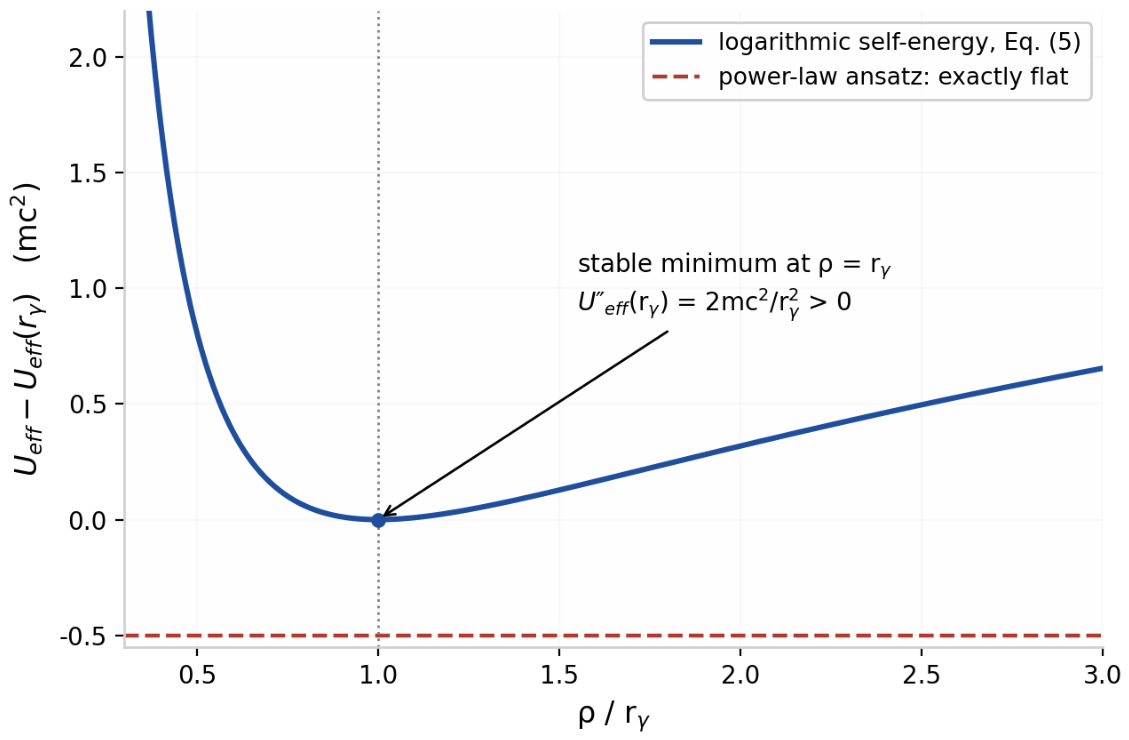
Figure 3.
The double-helix ontology of an entangled pair. The two quanta counter-circulate about the common axis with mirror-locked parameters (Equation (23)); the pair is one extended object until an interaction breaks it. The whole-pair variables (α1, φ1) cannot be assigned to either wing separately, which places the construction outside the class of local hidden-variable models.
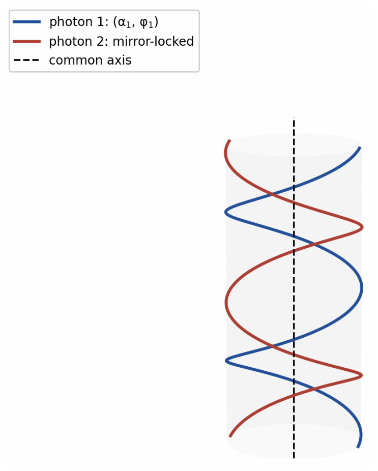
Figure 4.
The discriminating scaling of Section 8.1. The SSM detection profile is ring-supported with an on-axis void of diameter λ/π, locked to the wavelength and independent of numerical aperture; the Airy profiles (NA = 0.9, 0.5, 0.1) shrink with NA. The Airy radius falls below the void radius only for NA ≳ 3.8, so an NA scan at fixed wavelength separates the two structures at any achievable aperture.
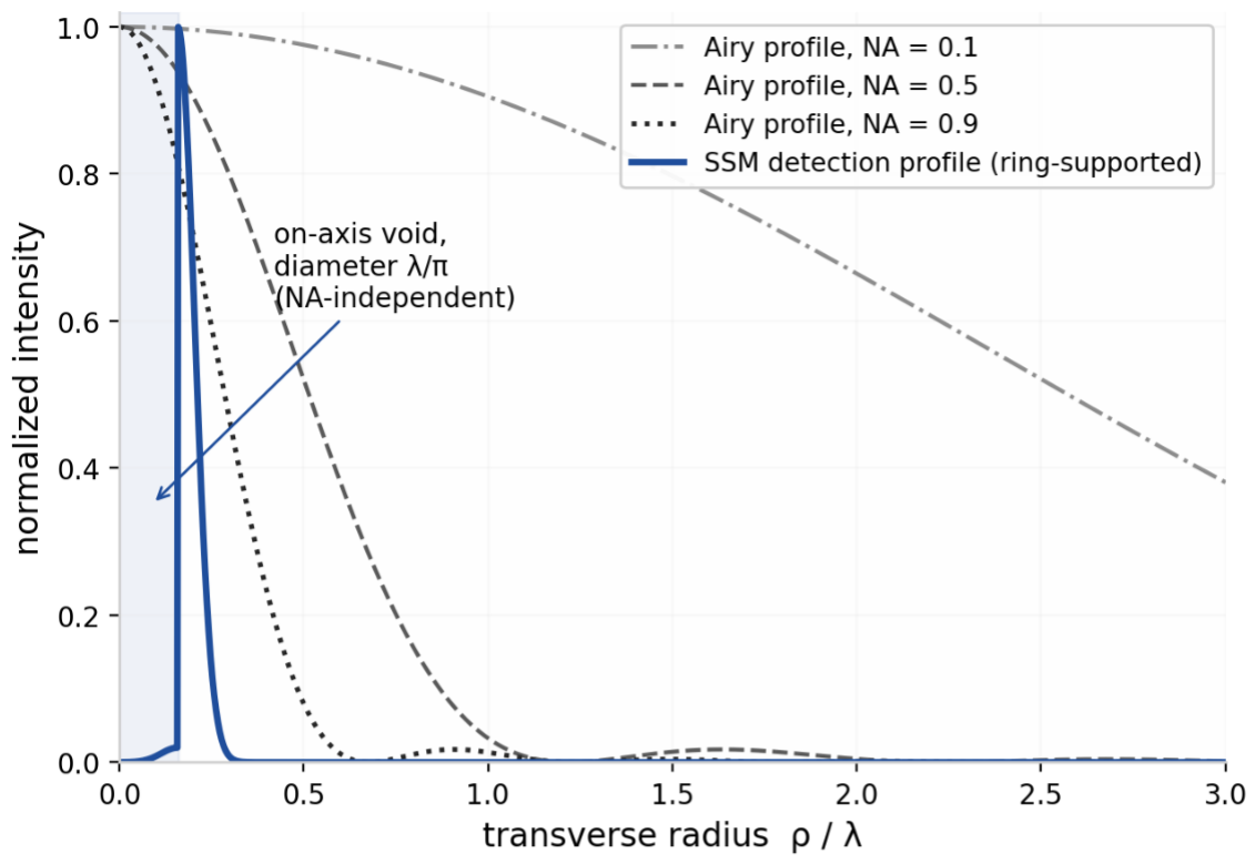
Table 1.
The three velocities of the helical photon and their distinct physical roles.
| Velocity | Value | Physical role |
| Signal (axial) vz | c | Carries the translational momentum p = mc and the energy flux; alone enters E = pc |
| Circulation (azimuthal) v⊥ | c | Internal rotation; contributes the angular momentum but no translational energy, exactly as the rim speed of a spinning rigid body contributes rotational but not translational kinetic accounting |
| Geometric arc-rate | √2 c | Arc-length parameter of the trajectory image; pure bookkeeping, since nothing physical propagates along the wire of the helix |
Table 2.
Sensitivity of the hydrogenic 1s binding energy to the regularization exponent n, under the static implementation of Equation (22). The spectroscopic tolerance at Z = 92 is |ΔB| ≲ 10 eV [26]. All entries independently recomputed for this revision.
Table 2.
Sensitivity of the hydrogenic 1s binding energy to the regularization exponent n, under the static implementation of Equation (22). The spectroscopic tolerance at Z = 92 is |ΔB| ≲ 10 eV [26]. All entries independently recomputed for this revision.
| Z | BDirac (keV) | ΔB, n = 4 (keV) | ΔB, n = 6 (keV) | ΔB, n = 8 (keV) |
| 26 | 9.28 | −0.012 | < 0.001 | < 0.001 |
| 54 | 41.35 | −1.03 | −0.161 | −0.025 |
| 82 | 101.58 | −13.5 | −5.09 | −1.86 |
| 92 | 132.28 | −27.6 | −13.4 | −6.23 |
Table 4.
Epistemic stratification of the framework’s claims, including components considered and excluded on the framework’s own criteria.
Table 4.
Epistemic stratification of the framework’s claims, including components considered and excluded on the framework’s own criteria.
| Claim | Status | Location |
| Observable-level relativistic kinematics; E = pc intact | Postulate with status statement [P] | Section 2.1 |
| Velocity-composition argument for composite speed c | Not adopted: two-body formula misapplied | Section 2.1 |
| mcrγ = ℏ for the helical photon, anchored in L = E/ω | Conditional theorem [T] | Section 2.1 and Section 2.2 |
| Logarithmic vortex confinement; stable minimum at rγ; ωrad = √2 ω; zero free parameters | Model [M] | Section 3.1 |
| Power-law r−2 confinement ansatz | Excluded: neutral or unstable equilibrium | Section 3.1 |
| rγ = λ/(2π); circulation identified with spin; no longitudinal mode | Theorem within model [T/M] | Section 3.2 |
| Orbital angular momentum an ensemble-level collective property | Model [M]; single-event mode sorting open (problem 10) | Section 3.2 |
| Quantized transverse vortex mode | Excluded: spin–orbit conflation | Section 3.2 |
| Two-slit fringes from phase-boundary coupling; edge shift δφ ∼ 2πrγ/a | Model [M], testable [F] | Section 3.3 |
| Malus law from explicit projection postulate; single events via entry phase | Assumption [M] + theorem [T, conditional] | Section 3.4 |
| Geometric uncertainty saturates ℏ/2 exactly (phase ensemble) | Theorem [T, ensemble] | Section 3.5 |
| Earlier (√2 − 1)ℏ ≈ 0.414ℏ estimate | Excluded: systematic offset is not a statistical width | Section 3.5 |
| 720-degree S-motion; spin ℏ/2; homotopy anchor | T (math) + M (mapping rule) | Section 4.1 |
| g = 2 | Input [M]; derivation open (problem 6) | Section 4.2 |
| Fermi statistics | Not addressed; open problem 8 | Section 4.1 and Section 9.2 |
| α = re/a0 | Identity [I], interpretive | Section 5.1 |
| Fine-structure splitting ∼ α4mc² | Model [M], order-of-magnitude | Section 5.2 |
| Free radiation field as ensemble moment; wave equation and transversality | Model [M] with one adjustable constant | Section 5.3 |
| Static xn regularization ansatz at Z = 137 | Excluded by data | Section 6.2 |
| Double-helix ontology with whole-pair variables; CHSH S = 2√2 | Model [M], consistency [T]; non-local realism | Section 7 |
| Lorentz covariance of the medium | Postulated [P]; envelope stated | Section 2.5 |
| Intrinsic on-axis void, λ-locked, NA-independent | Falsifiable prediction [F]; kinematics of Postulate I | Section 8.1 |
| Spin-dependent form-factor window at Q = mc | Falsifiable [F]; bounded by Mott polarimetry | Section 8.2 |
| Pair-coincidence periodicity at T = 1/ν | Falsifiable prediction [F] | Section 8.3 |
Disclaimer/Publisher’s Note: The statements, opinions and data contained in all publications are solely those of the individual author(s) and contributor(s) and not of MDPI and/or the editor(s). MDPI and/or the editor(s) disclaim responsibility for any injury to people or property resulting from any ideas, methods, instructions or products referred to in the content. |
© 2026 by the authors. Licensee MDPI, Basel, Switzerland. This article is an open access article distributed under the terms and conditions of the Creative Commons Attribution (CC BY) license (http://creativecommons.org/licenses/by/4.0/).
Copyright: This open access article is published under a Creative Commons CC BY 4.0 license, which permit the free download, distribution, and reuse, provided that the author and preprint are cited in any reuse.