
Submitted:
11 September 2026
Posted:
14 September 2026
You are already at the latest version
Abstract
Microbial source tracking (MST) estimates the contributions of candidate source communities to an observed sink community. However, taxon-aligned approaches can degrade when biological turnover or technical differences introduce "drift" between source and sink profiles, because abundance on related but nonmatching taxa is treated as separate features. We present MARSH, a phylogeny-aware MST framework that models source attribution as constrained optimal transport on the microbial tree using the tree-Wasserstein distance. By leveraging evolutionary structure, MARSH allows abundance to be matched across closely related taxa rather than enforcing strict feature identity. The formulation limits the loss to local tree structure so that broad clade-level differences do not dominate the fit, and it estimates unobserved contribution from the residual left by the named-source mixture. Across synthetic and real 16S rRNA benchmarks, MARSH attains the lowest mean attribution error in every evaluated drift condition and remains competitive in the no-drift settings. These results show that integrating tree geometry into community deconvolution can improve source tracking when ecological or experimental drift preserves local phylogenetic structure.
Keywords:
microbial source tracking
; optimal transport
; phylogen
1. Introduction
Microbial community assembly reflects interacting processes that include dispersal, selection, diversification, and ecological drift [1]. An observed community may also contain microbial contributions from several distinct sources. Understanding these contributions is important in settings where the origin of a community carries biological, environmental, or public-health significance. Microbial source tracking (MST) provides a framework for this task by estimating the relative contributions of candidate source communities to a target, or “sink,” community [2,3]. MST has been used to identify sources of fecal contamination in recreational and environmental waters, where distinguishing human, animal, wastewater, and other inputs can inform pollution control and water-quality management [4,5]. It has also been applied to trace microbial contamination and dispersal in hospitals, laboratories, offices, and other built environments [2,6], and to study the formation of host-associated microbiomes, including the contributions of maternal and early-life communities to the developing infant gut [3]. More broadly, source attribution provides a way to move beyond describing which microbes are present and ask where an observed community came from.
In a typical MST analysis, each source and sink is represented by its relative-abundance profile, and the goal is to estimate the fraction of the sink attributable to each candidate source [2,3]. These profiles are compositional because sequencing data describe the abundance of each taxon relative to the total observed community rather than providing independent absolute abundances [7]. Source attribution is further complicated by the fact that the reference library may not contain every community that contributed to the sink. An environmental or host-associated sample, for example, may contain input from an unsampled reservoir or from a source that was not included when the reference panel was constructed. MST methods must therefore estimate the contributions of the available sources while also allowing part of the sink to originate from an unknown source [2,3].
Beyond incomplete source libraries, MST can also be affected when the microbial composition of the sink no longer aligns exactly with that of the reference sources. We refer to this source–sink mismatch as drift. Drift can arise biologically as microbial communities change over time [8], or technically when source and sink samples are characterized using different 16S regions, primers, or sequencing protocols [9]. In either case, taxa observed in the sink may differ from those in the references even when they are phylogenetically related. Existing MST approaches based on Bayesian mixture models, expectation–maximization, and matrix factorization operate on a shared feature space and match abundance across corresponding taxa [2,3,10]. They therefore cannot directly use the relationship between a taxon present in the sink and a closely related taxon present in a source. As drift increases, this mismatch can lead source contributions to be misestimated or attributed to the unknown component.
Phylogeny provides a natural way to incorporate this relationship. Phylogenetic community distances were developed to distinguish changes among close relatives from changes across deeper lineages [11,12]. Optimal transport makes this distinction explicit by treating microbial communities as probability measures on a phylogenetic tree. In this setting, the tree-based Wasserstein-1, or Kantorovich–Rubinstein, distance coincides with raw weighted UniFrac and has a closed-form edge-sum representation on the tree [12,13]. Transport between nearby taxa therefore costs less than transport between taxa separated by long phylogenetic distances. MARSH uses this geometry directly in the source-mixture estimation problem, allowing phylogenetically local differences between the sink and its references to be treated as drift rather than automatically as evidence for a different or unknown source. Our contributions are threefold:
- 1.
- We formulate MST as a constrained optimal-transport problem on the phylogenetic tree, estimating source mixing weights by minimizing the tree-Wasserstein distance between the source mixture and the sink. The resulting problem is solved as an exact least-absolute-deviations linear program (Section 3.4).
- 2.
- We introduce a fixed locality rule that limits the loss to shallow phylogenetic structure. This preserves the ability to match locally drifted taxa while preventing broad clade-level imbalances from dominating the fit (Section 3.3).
- 3.
- We introduce an estimator of the unknown-source fraction based on the residual mismatch after fitting the known sources. It is designed to distinguish unexplained source contribution from mismatch that can be explained by local phylogenetic drift (Section 3.5).
We evaluate these components against FEAST, SourceID-NMF, and FastST on simulated and real 16S data, including unknown sources, induced phylogenetic drift, and naturally occurring temporal drift.
2. Related Work
Most quantitative microbial source tracking methods begin from the standard mixture assumption. Let denote the observed sink, let denote candidate source profiles over the same n taxa, and let denote their mixing proportions. In its simplest form, MST assumes that the expected sink composition can be written as
Methods differ primarily in how the source profiles are modeled, how an unobserved source is represented, and what statistical discrepancy is used to compare the mixture with the sink. The methods considered below all use a common taxonomic feature space: taxon j in the sink is modeled through abundance associated with taxon j in the sources. Some methods couple residuals across taxa statistically, but none of these formulations assigns a smaller mismatch cost merely because two different taxa are phylogenetically close. We summarize the main mathematical approaches to MST below.
One influential approach is the Bayesian mixture model used by SourceTracker [2], which formulates MST as a hierarchical Bayesian mixture model at the sequence level. Let denote the taxon distribution of source environment k, and let denote the proportions of the source environments in the sink. For sink read r, the model introduces a latent source assignment :
Reference-source observations update the corresponding , while Gibbs sampling integrates uncertainty in both source-specific taxon frequencies and sink mixing proportions. An additional source category represents taxa attributable to an unobserved environment.
The categorical likelihood has taxon-specific support. If sink read r is observed as taxon j, then under source k its likelihood is
Thus, the model can use the probability assigned to taxon j by a source, but it contains no term involving the relationship between j and another taxon . A source with abundance at a close phylogenetic relative receives no special credit unless that relationship is already reflected in the shared taxon frequencies themselves.
FEAST [3] instead uses a maximum-likelihood mixture model. It retains the probabilistic mixture formulation but replaces Markov-chain Monte Carlo inference with expectation–maximization. Let be sink counts with total count , and let be the observed counts for known source k with total . FEAST introduces source-specific relative-abundance vectors and mixing proportions , including an additional unobserved source. The sink probabilities are
The generative model is
Up to terms independent of the unknown parameters, the joint log-likelihood is
The first term fits the source mixture to the sink, while the second anchors the known latent source profiles to their observed reference counts. For fixed source profiles, maximizing the sink term is equivalent, up to an additive constant and a factor of C, to minimizing
where is the Kullback–Leibler divergence.
The taxon alignment becomes particularly clear in the EM responsibility for assigning abundance of taxon j to source k:
Only the abundance of the same taxon j enters this assignment. Abundance at a phylogenetically nearby taxon cannot directly explain the observation at j.
SourceID-NMF [10] uses non-negative matrix factorization to relax the assumption that the taxonomic profile of a source in the sink must be identical to its observed reference profile. Let denote the sink, let contain the reference source profiles, and let and denote the latent source profiles and their proportions, respectively. The final column corresponds to an unknown source and is masked from the reference penalty by A. SourceID-NMF solves
where ∘ denotes the Hadamard product. The problem is optimized using the alternating direction method of multipliers.
This formulation is more flexible than fixing the source profiles to Y: the latent profile can deviate from the observed reference . However, both terms remain Euclidean in the taxon coordinates. In particular,
and
Changing a source profile from taxon i to taxon j is therefore not assigned a cost based on the biological distance between i and j. A transfer between two closely related taxa and a transfer between distant clades are distinguished only through the resulting numerical changes in the abundance vectors.
FastST [14] takes a generalized least-squares approach, starting from the same multinomial mixture relation
where denotes an unobserved source. Instead of jointly estimating the source taxon distributions and mixing proportions iteratively, it treats the known as given, or estimates them from the observed source frequencies. Multiplying (15) by the sink sequencing depth C gives
Because both the abundance profile and proportion of the unobserved source are unidentified, FastST assumes that is constant across taxa. Defining the resulting unknown-source term as an intercept and setting for the observed sources gives the linear model
Under the multinomial model,
FastST estimates this covariance from the sink and uses generalized least squares. Writing and the estimated covariance as , the estimator takes the form
where denotes an inverse after removing the multinomial singularity or, equivalently, a Moore–Penrose pseudoinverse.
Unlike a simple coordinate-wise squared-error loss, GLS accounts for the negative covariance among multinomial taxon counts through . Nevertheless, the design matrix remains taxon-aligned: predicts sink abundance at taxon j. The covariance structure models statistical dependence among residuals but does not encode phylogenetic distance between taxon j and another taxon .
Taken together, existing MST methods provide distinct probabilistic and optimization-based formulations for estimating source contributions, including Bayesian inference, maximum-likelihood estimation, matrix factorization, and generalized least squares. Although these approaches differ in their treatment of uncertainty, unknown sources, and computation, they represent sources and sinks on a shared taxonomic feature space and do not explicitly account for phylogenetic distance between nonmatching taxa. Conversely, phylogenetic distances such as weighted UniFrac incorporate evolutionary relatedness when comparing microbial communities [11,12,13], but do not by themselves provide a source-mixture estimator. This separation between source attribution and phylogenetic community comparison motivates a formulation that brings the two together.
3. Methods
MARSH estimates the contributions of candidate microbial sources to an observed sink by fitting a mixture model under a phylogeny-aware transport loss. We first define the source-tracking problem and its unknown-source component, then introduce the phylogenetic discrepancy used by MARSH, its locality modification, and the resulting estimators.
3.1. Problem Formulation
Let the observed sink community contain counts over n taxa, with total sequencing depth . We work with the corresponding relative-abundance profile
The reference panel contains K candidate source communities with relative-abundance profiles . The basic MST task is to estimate the proportion of the sink contributed by each of these sources.
Because the reference panel may not contain every community that contributed to the sink, we also allow an unknown source with profile and contribution . We model the sink as
where gives the relative proportions of the named sources within the explained component of the sink. The final contribution of named source k is therefore .
The inputs to MARSH are the sink profile , the candidate source profiles , and, when available, a phylogenetic tree T relating the observed taxa. The outputs are the estimated named-source contributions and, when unknown-source estimation is enabled, the unknown fraction and estimated profile .
The sink and its reference sources need not agree exactly at the taxon level. Under phylogenetically local drift, abundance associated with a source taxon may instead appear at a nearby relative in the sink. A discrepancy based only on matching corresponding taxa treats such a change as an ordinary mismatch and ignores the relationship between the two taxa. MARSH therefore fits the mixture in Eq. (21) using a phylogenetic transport loss, so that mismatches between closely related taxa incur a smaller cost than mismatches between distantly related taxa.
3.2. Phylogenetic Transport Loss
Let T be a rooted phylogenetic tree whose leaves correspond to the n taxa, with edge set E and edge lengths . For edge e, let denote the set of descendant taxa and define the cumulative mass below that edge as
Optimal transport compares two distributions by asking how much mass must be moved, and how far, to transform one distribution into the other [15,16]. When the transport cost between taxa i and j is their patristic distance on the phylogeny, the Wasserstein-1 distance is
where is the set of non-negative transport plans with marginals and .
On a tree, this optimization has the closed form
This quantity is the phylogenetic Kantorovich–Rubinstein distance and is equivalent to raw weighted UniFrac for normalized communities [12,13]. Equation (24) provides the key property needed for source tracking: a mismatch between nearby taxa contributes only the length of the short path separating them, whereas a mismatch between distant taxa incurs a larger cost.
The tree representation is also computationally useful. Since each is linear in , the tree-Wasserstein distance is a weighted norm of a linear transformation of . This allows the source-mixture problem to be written directly as a linear program.
3.3. Local Phylogenetic Transport
Full tree-Wasserstein distance incorporates structure at every phylogenetic scale. This is desirable when source–sink differences occur among nearby taxa, but deep edges can also give substantial weight to differences between large clades. For source attribution, we therefore restrict the phylogenetic contribution of the loss to local tree structure.
Let
and retain only edges whose descendant subtree contains at most h taxa. Define
The resulting local tree loss is
This modification retains all leaf edges and shallow internal edges. Exact taxonomic mismatches therefore remain penalized, while shallow internal edges provide partial tolerance when abundance shifts among nearby phylogenetic relatives. Deep edges are excluded so that broad clade-level imbalances do not dominate the source-mixture fit. The cutoff depends only on the number of taxa represented by the tree and introduces no drift-dependent tuning parameter.
3.4. Estimating the Named-Source Proportions
For each edge e and source k, define
For a candidate mixture , linearity gives
The named-source weights are therefore estimated by
Introducing one auxiliary variable for each retained edge gives the least-absolute-deviations linear program
The problem contains variables and a number of constraints linear in the number of tree edges, and can therefore be solved directly with a standard linear-programming solver.
When no phylogenetic tree is supplied, the taxa are attached to a flat star scaffold. For the fully observed estimator, this makes the tree-Wasserstein objective equal to coordinate-wise distance. When the unknown-source estimator is enabled without a phylogenetic tree, its weight update instead uses simplex-constrained least squares. Define and for . Conditional on the current unknown profile, the update is
This weight update alternates with a soft responsibility update of until the weights converge. The residual-based procedure below is used when a phylogenetic tree is supplied. An optional reweighted sparsity penalty may be added when the candidate source library is large; all default experiments use unless otherwise specified.
3.5. Residual-Based Unknown-Source Estimation with a Phylogenetic Tree
Estimating an unknown source introduces an identifiability problem. A discrepancy between the sink and the named-source mixture can arise either because a genuine source is absent from the reference panel or because a known source has changed relative to its reference profile. Treating every unexplained taxon as unknown therefore risks confusing drift with a missing source.
We first fit only the named sources and define
where R is the residual discrepancy that cannot be eliminated by reweighting the named sources.
We construct a candidate unknown-source profile from the positive taxonomic residual,
where renormalizes a non-zero vector to the simplex. If the residual is zero, we set and no unknown profile is required.
The transport loss has a useful scaling property. For any ,
Thus, if the residual were generated entirely by mixing an unknown profile into the named mixture, its fraction would naturally scale as . Under heavy drift, however, the residual profile may lie very close to the named mixture, making this denominator small and causing the ratio to overestimate the unknown fraction. We therefore introduce the intrinsic source-separation scale
and estimate
The floor prevents a small residual-to-mixture distance from producing a large unknown estimate and is determined entirely by the observed source geometry rather than by a tuned threshold.
After estimating and , we remove the estimated unknown contribution,
and refit the named-source weights. In our implementation this update is repeated for three rounds, after which the reported source proportions are
The distinction between drift and an unknown source follows directly from the geometry of the loss. If an amount of mass is displaced from taxon to taxon , then
where is the path cost induced by the retained tree edges. Drift between nearby taxa therefore produces a small residual, whereas source mass that cannot be reconciled with the named mixture produces a larger residual. This distinction is not absolute: an unknown source that is itself phylogenetically similar to the named sources may also produce a small transport residual. We return to this identifiability limit in Section 6.
3.6. Uncertainty
For fits without an unknown source, we quantify sampling uncertainty with a multinomial bootstrap. Given sink counts at sequencing depth N, bootstrap replicate b is drawn as
Each reference source is independently resampled in the same way at its observed sequencing depth. The resampled profiles are renormalized and the estimator is rerun to obtain . A confidence interval for each estimated proportion is given by the empirical percentile interval
where denotes the empirical q-quantile of the corresponding B bootstrap estimates. The current implementation reports point estimates, but not bootstrap intervals, when the unknown-source estimator is enabled.
4. Experimental Design
We evaluate MARSH on simulated and real 16S data under three settings: fully observed sources, unknown sources, and source–sink drift. The simulated experiments provide controlled ground truth, while the real-data experiments use observed microbial communities and taxonomy.
4.1. Simulated Data
Each simulated replicate is generated using our export-sim tool. We first draw a random birth–death phylogeny with n leaves and positive edge lengths. For sources, the source profiles are sampled as
Ground-truth mixing weights are then selected. When an unknown source is included, we also generate an unknown profile with fraction . The sink distribution is formed using Eq. (21), and observed counts are sampled as
Thus, all methods operate on finite-depth count data rather than the underlying probability vectors.
Three controlled evaluations use this generator. The fully observed scaling evaluation (Section 5.1) uses and . The unknown-source evaluation without drift (Section 5.2) fixes and varies the unknown fraction . The simulated drift evaluation (also Section 5.2) fixes and . Each condition is repeated over five independent replicates.
4.2. GlobalPatterns
We use the GlobalPatterns 16S dataset [17], processed using QIIME 2 and phyloseq [18]. The dataset contains eight environment types: Feces, Skin, Tongue, Freshwater, Freshwater (creek), Ocean, Sediment (estuary), and Soil. Samples from each environment are pooled to form a source profile .
After filtering low-prevalence taxa, taxa remain. The accompanying phylogeny is midpoint-rooted. For the drift experiment, we use a -taxon subtree to reduce the cost of repeated tree-based optimization. We use a leave-one-environment-out design. For each environment U, we remove U from the candidate source set and construct the sink from two retained environments, A and B, together with the withheld environment:
The true sink contributions are , , and . The environments A and B are selected using a fixed random seed. The remaining candidate set contains seven environments, including five zero-weight distractors. Since U is withheld from the candidate set, its contribution can only be recovered through the unknown-source estimate. Repeating this procedure for all eight environments gives eight paired trials. The no-drift and genus-drift evaluations are reported in Section 5.3.
4.3. Drift Models
We evaluate two forms of drift. The simulated drift evaluation (Section 5.2) uses the TADA generative model [19] to introduce structured phylogenetic perturbations in the sink. For the GlobalPatterns evaluation (Section 5.3), we define taxonomy-based genus turnover. Each eligible reference taxon i is paired with a source-absent taxon from the same genus. At drift level f, a fraction of the abundance at taxon i is transferred to its congener:
The profile is renormalized after all transfers. At , no drift is applied, while at half of each affected reference taxon’s mass is transferred to its congener. The mapping is defined using genus annotations rather than distances on the phylogenetic tree used by MARSH. The drift construction is therefore independent of the tree used by the estimator. For both simulated and real data, drift is evaluated at ; we do not evaluate or claim behavior beyond .
4.4. Baselines and Evaluation
We compare MARSH with the published implementations of FEAST [3], SourceID-NMF [10], and FastST [14]. FEAST is run using its R implementation, SourceID-NMF using its Python implementation with 300 iterations, and FastST using its R implementation.
Accuracy is measured using the error between the estimated and true source proportions:
where denotes the unknown-source fraction. Lower values indicate more accurate source recovery.
Simulated results are reported descriptively as means over five independent replicates. Real-data results use paired observations from the eight leave-one-environment-out trials or the 27 Moving Pictures sinks. We compare real-data errors using two-sided paired Wilcoxon signed-rank tests [20]. The two external-method comparisons in each single-condition real-data evaluation are adjusted together using the Benjamini–Hochberg procedure [21]. For the five-level GlobalPatterns drift sweep, the five p-values for each of the two external comparators are combined into one family of ten tests for Benjamini–Hochberg adjustment. Adjusted values are reported as q-values. Exact permutation p-values are computed from the signed-rank statistic using midranks for tied absolute differences; differences smaller than are treated as numerical ties. In the real-data tables, superscripts indicate p- or q-value thresholds: *, **, and ***. No superscript indicates a non-significant difference. The leave-one-environment-out tests quantify consistency across the eight GlobalPatterns environments rather than population-level uncertainty. The Moving Pictures tests treat sinks as the paired analysis units but do not model temporal dependence among repeated samples from the same body site, so those p-values are interpreted as exploratory.
5. Results
5.1. Simulated Data with Fully Observed Sources Across Taxon Counts
No phylogenetic tree is supplied to MARSH in this experiment. With all sources known and no unknown, MARSH is competitive with the best baseline on small tables and attains the lowest mean error as dimensionality grows, while FEAST and SourceID-NMF degrade (Table 1). MARSH and FastST trade the lowest mean error across the sweep: FastST leads at 50 and 500 taxa, while MARSH leads at and taxa.
5.2. Simulated Data with an Unknown Source
We first consider the simulated unknown-source setting without drift. No phylogenetic tree is supplied to MARSH for this evaluation. As the true unknown fraction increases from to , MARSH attains the lowest error at every level (Table 2). FEAST’s error grows sharply as it misattributes the missing mass, while SourceID-NMF trails without leading.
We then introduce TADA drift while holding the true unknown fraction at . A phylogenetic tree is supplied to MARSH. Its error remains near and is lowest at every drift level (Table 3, Figure 1(a)). The transport loss carries drifted mass back to the correct source, while the floored denominator limits inflation of the estimated unknown fraction when the residual profile lies close to the named-source mixture.
5.3. GlobalPatterns Data with an Unknown Source
We first evaluate GlobalPatterns without drift. No phylogenetic tree is supplied to MARSH in this setting. With one environment withheld as an unknown source with a true fraction of , MARSH recovers the unknown fraction as and attains an order of magnitude lower error than the best competitor (Table 4). Two-sided paired Wilcoxon signed-rank tests give against each competitor, with all eight trials favoring MARSH.
We next introduce genus drift. A phylogenetic tree is supplied to MARSH for this evaluation. Across , MARSH’s error rises from to but remains the lowest throughout (Table 5, Figure 1(b)). SourceID-NMF degrades from to as exact matching fails, while FEAST’s error changes from to . After Benjamini–Hochberg correction across all ten external-method comparisons in the drift sweep, the two-sided paired Wilcoxon tests give for both external methods at –. At , the tests give for FEAST and for SourceID-NMF.
5.4. Moving Pictures Data with Natural Temporal Drift
We evaluate naturally occurring drift using the QIIME 2 Moving Pictures dataset [8], in which the same body sites (gut, tongue, palm) are sampled repeatedly over months. We take each body site’s day-0 community as its source and attribute each later sample (days 84–168) to its body site; the sink has drifted from its own day-0 reference through real turnover, not a synthetic perturbation. Scoring each attribution against its true body site by (Table 6, sinks), MARSH attains the lowest mean error. Sink-level two-sided paired Wilcoxon tests give versus FEAST and versus SourceID-NMF; these comparisons are exploratory because temporal dependence within body sites is not modeled. Unlike the induced genus drift, natural gut turnover is dominated by phylogenetically distant novel taxa rather than local congener movement. A phylogenetic tree is supplied to MARSH for the primary evaluation, which produces an error of ; omitting the tree produces an error of , and the difference is not significant (two-sided paired Wilcoxon, ). The locality-bounded metric (Section 3.3) avoids the higher mean error observed with an unrestricted tree-Wasserstein loss, which raises MARSH’s error to , while the locality-bounded loss preserves its large advantage under phylogenetically local drift (Table 3 and Table 5).
5.5. Runtime and Peak Memory on Simulated and GlobalPatterns Data
Figure 2 summarizes computational scaling on the fully observed simulated data. Without a phylogenetic tree, MARSH is the fastest method through taxa. At taxa its runtime rises to seconds because the coordinate-wise linear program grows with the number of taxa; it remains faster than FastST but is slower than FEAST and SourceID-NMF. MARSH has the lowest measured peak memory at every table size, using MB at taxa.
On the full GlobalPatterns input with taxa and seven candidate sources, MARSH was run with a phylogenetic tree and unknown-source estimation. It took seconds, compared with – seconds for the external methods, while using less peak memory: MB compared with – MB.
6. Discussion
The experiments show that phylogenetic information is most useful when source and sink profiles differ through local taxonomic replacement. In the simulated TADA and GlobalPatterns genus-drift evaluations (Table 3 and Table 5), tree-Wasserstein distance maps abundance discrepancies along local evolutionary paths [12,13]. The fixed locality cutoff (, Section 3.3) limits the distance calculation to shallow subtree edges, allowing drifted congener counts to remain associated with their reference sources. In the Moving Pictures temporal-drift evaluation (Section 5.4), the paired comparison does not detect an error difference between fits with and without a phylogenetic tree, while MARSH retains its advantage over the external baselines. Under heavier drift, the denominator floor prevents collapsed transport distances from inflating the estimated unknown fraction. Together, these results support tree-based optimal transport as a practical, geometry-aware basis for community deconvolution [15,16].
The results also expose several operational trade-offs. When an unobserved source is phylogenetically adjacent to a candidate reference, transport partially absorbs missing mass as local drift, leading to a modest underestimation of the unknown fraction. Integrating multi-sample temporal tracking or lineage-specific priors could resolve this boundary by separating static ancestral divergence from rapid phenotypic drift. Because tree transport assigns low cost to short paths, it can also blur fine differences between near-identical strain variants; hierarchical loss schedules that enforce exact coordinate matching at the leaves while using tree transport across internal nodes could preserve both strain-level precision and clade-level drift tolerance. The present drift evaluations use synthetic perturbations and a congener-enriched panel (92% coverage) to probe the local-transport regime. Benchmarking on field cohorts with diverse, uncurated environmental drift will further map performance across broad taxonomic scales.
The largest simulated evaluation indicates that runtime, rather than memory, is the immediate scaling constraint. A matrix-free primal–dual solver could exploit the convex weighted- form without constructing the full linear-program constraint matrix; such methods are established for large structured nonsmooth convex problems [22].
Future development will focus on adapting the optimization framework to incorporate relevant biological priors and information, including phylogenetic tree structure, lineage-specific evolutionary rates, sequencing depth, and temporal or environmental context. These additions could make the model more responsive to differences among microbial systems while preserving a common source-tracking framework. Evaluating MARSH across longitudinal environmental systems, including wastewater surveillance, infant gut colonization, and industrial bioreactor tracking, will test its utility across diverse ecological succession dynamics.
7. Conclusion
MARSH reframes microbial source tracking as constrained optimal transport under the tree-Wasserstein metric, coupling phylogenetic geometry with a residual-anchored unknown-source estimator. Across synthetic drift benchmarks and real 16S rRNA genus turnover, this approach attains lower mean attribution errors than the evaluated coordinate-wise mixture and matrix-factorization baselines at every tested drift level. Limiting the loss to local tree structure improves attribution under the evaluated feature-level drift without the higher mean error observed for unrestricted tree-Wasserstein loss under broad turnover. The denominator floor limits inflation of the unknown-source estimate, and the no-drift evaluations support recovery of withheld-source contributions. Future development will focus on adapting the optimization framework to incorporate relevant biological priors and information, including phylogenetic tree structure, lineage-specific evolutionary rates, sequencing depth, and temporal or environmental context.
Source code and scripts reproducing all tables and figures are available at https://github.com/advaitb/MARSH.
References
- Nemergut, D.R.; Schmidt, S.K.; Fukami, T.; O’Neill, S.P.; Bilinski, T.M.; Stanish, L.F.; Knelman, J.E.; Darcy, J.L.; Lynch, R.C.; Wickey, P.; et al. Patterns and processes of microbial community assembly. Microbiol. Mol. Biol. Rev. 2013, 77, 342–356. [Google Scholar] [CrossRef] [PubMed]
- Knights, D.; Kuczynski, J.; Charlson, E.S.; Zaneveld, J.; Mozer, M.C.; Collman, R.G.; Bushman, F.D.; Knight, R.; Kelley, S.T. Bayesian community-wide culture-independent microbial source tracking. Nat. Methods 2011, 8, 761–763. [Google Scholar] [CrossRef] [PubMed]
- Shenhav, L.; Thompson, M.; Joseph, T.A.; Briscoe, L.; Furman, O.; Bogumil, D.; Mizrahi, I.; Pe’er, I.; Halperin, E. FEAST: fast expectation-maximization for microbial source tracking. Nat. Methods 2019, 16, 627–632. [Google Scholar] [CrossRef] [PubMed]
- Field, K.G.; Samadpour, M. Fecal source tracking, the indicator paradigm, and managing water quality. Water Res. 2007, 41, 3517–3538. [Google Scholar] [CrossRef] [PubMed]
- Henry, R.; Schang, C.; Coutts, S.; Kolotelo, P.; Prosser, T.; Crosbie, N.; Grant, T.; Cottam, D.; O’Brien, P.; Deletic, A.; et al. Into the deep: Evaluation of SourceTracker for assessment of faecal contamination of coastal waters. Water Res. 2016, 93, 242–253. [Google Scholar] [CrossRef] [PubMed]
- Flores, G.E.; Bates, S.T.; Knights, D.; Lauber, C.L.; Stombaugh, J.; Knight, R.; Fierer, N. Microbial biogeography of public restroom surfaces. PLoS ONE 2011, 6, e28132. [Google Scholar] [CrossRef] [PubMed]
- Gloor, G.B.; Macklaim, J.M.; Pawlowsky-Glahn, V.; Egozcue, J.J. Microbiome datasets are compositional: and this is not optional. Front. Microbiol. 2017, 8, 2224. [Google Scholar] [CrossRef] [PubMed]
- Caporaso, J.G.; Lauber, C.L.; Costello, E.K.; Berg-Lyons, D.; Gonzalez, A.; Stombaugh, J.; Knights, D.; Gajer, P.; Ravel, J.; Fierer, N.; et al. Moving pictures of the human microbiome. Genome Biol. 2011, 12, R50. [Google Scholar] [CrossRef] [PubMed]
- Tremblay, J.; Singh, K.; Fern, A.; Kirton, E.S.; He, S.; Woyke, T.; Lee, J.; Chen, F.; Dangl, J.L.; Tringe, S.G. Primer and platform effects on 16S rRNA tag sequencing. Front. Microbiol. 2015, 6, 771. [Google Scholar] [CrossRef] [PubMed]
- Huang, Z.; Cai, D.; Sun, Y. Towards more accurate microbial source tracking via non-negative matrix factorization (NMF). Bioinformatics 2024, 40, i68–i78. [Google Scholar] [CrossRef] [PubMed]
- Lozupone, C.; Knight, R. UniFrac: a new phylogenetic method for comparing microbial communities. Appl. Environ. Microbiol. 2005, 71, 8228–8235. [Google Scholar] [CrossRef] [PubMed]
- Lozupone, C.A.; Hamady, M.; Kelley, S.T.; Knight, R. Quantitative and qualitative β diversity measures lead to different insights into factors that structure microbial communities. Appl. Environ. Microbiol. 2007, 73, 1576–1585. [Google Scholar] [CrossRef] [PubMed]
- Evans, S.N.; Matsen, F.A. The phylogenetic Kantorovich–Rubinstein metric for environmental sequence samples. J. R. Stat. Soc. Ser. B (Statistical Methodology) 2012, 74, 569–592. [Google Scholar] [CrossRef] [PubMed]
- Choi, J.M.; Wu, X.; Zhang, L. FastST: an efficient tool for inferring decomposition and directionality of microbial communities. PeerJ 2025, 13, e20161. [Google Scholar] [CrossRef] [PubMed]
- Villani, C. Optimal Transport: Old and New. In Grundlehren der mathematischen Wissenschaften; Springer, 2009; Vol. 338. [Google Scholar] [CrossRef]
- Peyré, G.; Cuturi, M. Computational Optimal Transport. Found. Trends Mach. Learn. 2019, 11, 355–607. [Google Scholar] [CrossRef]
- Caporaso, J.G.; Lauber, C.L.; Walters, W.A.; Berg-Lyons, D.; Lozupone, C.A.; Turnbaugh, P.J.; Fierer, N.; Knight, R. Global patterns of 16S rRNA diversity at a depth of millions of sequences per sample. Proc. Natl. Acad. Sci. 2011, 108, 4516–4522. [Google Scholar] [CrossRef] [PubMed]
- Bolyen, E.; Rideout, J.R.; Dillon, M.R.; et al. Reproducible, interactive, scalable and extensible microbiome data science using QIIME 2. Nat. Biotechnol. 2019, 37, 852–857. [Google Scholar] [CrossRef] [PubMed]
- Sayyari, E.; Kawas, B.; Mirarab, S. TADA: phylogenetic augmentation of microbiome samples enhances phenotype classification. Bioinformatics 2019, 35, i31–i40. [Google Scholar] [CrossRef] [PubMed]
- Wilcoxon, F. Individual comparisons by ranking methods. Biom. Bull. 1945, 1, 80–83. [Google Scholar] [CrossRef]
- Benjamini, Y.; Hochberg, Y. Controlling the false discovery rate: a practical and powerful approach to multiple testing. J. R. Stat. Soc. Ser. B (Methodological) 1995, 57, 289–300. [Google Scholar] [CrossRef]
- Chambolle, A.; Pock, T. A first-order primal–dual algorithm for convex problems with applications to imaging. J. Math. Imaging Vis. 2011, 40, 120–145. [Google Scholar] [CrossRef]
Figure 1.
Mean error for simulated TADA drift (a) and GlobalPatterns genus drift (b), each with a true unknown fraction of . MARSH attains the lowest at every evaluated drift level () on both datasets. On simulated data MARSH remains nearly constant across drift levels; on GlobalPatterns, SourceID-NMF error rises with drift while FEAST remains higher than MARSH.
Figure 1.
Mean error for simulated TADA drift (a) and GlobalPatterns genus drift (b), each with a true unknown fraction of . MARSH attains the lowest at every evaluated drift level () on both datasets. On simulated data MARSH remains nearly constant across drift levels; on GlobalPatterns, SourceID-NMF error rises with drift while FEAST remains higher than MARSH.
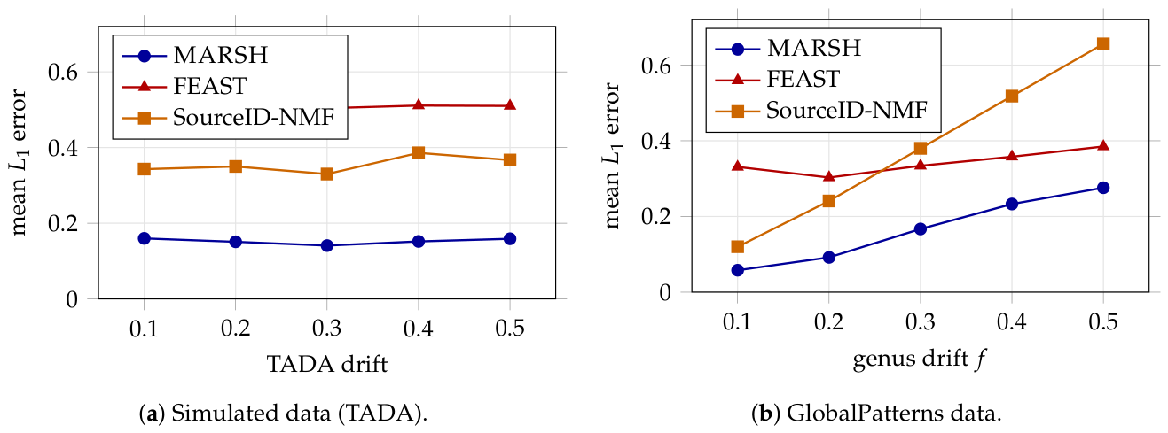
Figure 2.
Runtime and peak resident memory for the fully observed simulated scaling evaluation. Both axes use logarithmic scales. Lower values are better.
Figure 2.
Runtime and peak resident memory for the fully observed simulated scaling evaluation. Both axes use logarithmic scales. Lower values are better.
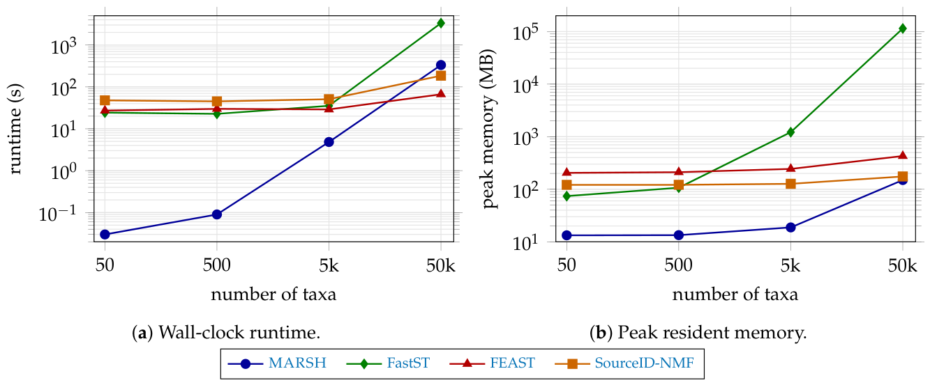

Table 1.
Fully observed sources, no unknown: mean error versus number of taxa (unknown fraction ). Best per row in bold.
Table 1.
Fully observed sources, no unknown: mean error versus number of taxa (unknown fraction ). Best per row in bold.
| # taxa | MARSH | FastST | FEAST | SourceID-NMF |
|---|---|---|---|---|
| 50 | 0.023 | 0.020 | 0.034 | 0.215 |
| 500 | 0.032 | 0.026 | 0.042 | 0.328 |
| 5,000 | 0.036 | 0.054 | 0.068 | 0.705 |
| 50,000 | 0.099 | 0.132 | 0.467 | 0.782 |
Table 2.
Simulated data with an unknown source and no drift: mean versus true unknown fraction.
| unknown | MARSH | FEAST | NMF |
|---|---|---|---|
| 0.2 | 0.172 | 0.347 | 0.357 |
| 0.4 | 0.159 | 0.707 | 0.234 |
| 0.6 | 0.209 | 1.062 | 0.265 |
| 0.8 | 0.299 | 1.418 | 0.343 |
Table 3.
Simulated TADA drift with an unknown source fraction of : mean .
| drift | MARSH | FEAST | NMF |
|---|---|---|---|
| 0.1 | 0.160 | 0.492 | 0.343 |
| 0.2 | 0.151 | 0.500 | 0.350 |
| 0.3 | 0.141 | 0.504 | 0.330 |
| 0.4 | 0.152 | 0.511 | 0.386 |
| 0.5 | 0.159 | 0.510 | 0.367 |
Table 4.
GlobalPatterns data with an unknown source fraction of and no drift.
| method | mean | rec. unknown |
|---|---|---|
| MARSH | 0.017 | 0.292 |
| NMF | 0.162** | 0.291 |
| FEAST | 0.251** | 0.175 |
Table 5.
GlobalPatterns genus drift with an unknown source fraction of : mean over .
| drift f | MARSH | FEAST | NMF |
|---|---|---|---|
| 0.1 | 0.058 | 0.331** | 0.120** |
| 0.2 | 0.092 | 0.303** | 0.241** |
| 0.3 | 0.167 | 0.334** | 0.380** |
| 0.4 | 0.233 | 0.358** | 0.518** |
| 0.5 | 0.276 | 0.385* | 0.656** |
Table 6.
Natural temporal drift in Moving Pictures: mean of body-site attribution ( sinks, truth the sink’s own site). Lower is better; significance is a Benjamini–Hochberg-adjusted two-sided paired Wilcoxon test against MARSH.
Table 6.
Natural temporal drift in Moving Pictures: mean of body-site attribution ( sinks, truth the sink’s own site). Lower is better; significance is a Benjamini–Hochberg-adjusted two-sided paired Wilcoxon test against MARSH.
| method | mean |
|---|---|
| MARSH | 0.92 |
| FEAST | 1.39* |
| SourceID-NMF | 1.92*** |
Disclaimer/Publisher’s Note: The statements, opinions and data contained in all publications are solely those of the individual author(s) and contributor(s) and not of MDPI and/or the editor(s). MDPI and/or the editor(s) disclaim responsibility for any injury to people or property resulting from any ideas, methods, instructions or products referred to in the content. |
© 2026 by the authors. Licensee MDPI, Basel, Switzerland. This article is an open access article distributed under the terms and conditions of the Creative Commons Attribution (CC BY) license (http://creativecommons.org/licenses/by/4.0/).
Copyright: This open access article is published under a Creative Commons CC BY 4.0 license, which permit the free download, distribution, and reuse, provided that the author and preprint are cited in any reuse.