

Submitted:
12 September 2026
Posted:
14 September 2026
You are already at the latest version
Abstract
This paper presents a novel advanced mathematical framework for motion planning of autonomous vehicles (AVs), centered on the simultaneous optimization of spatial trajectories and kinematic profiles within an augmented Frenet coordinate system. Addressing the inherent limitations of traditional two-stage planning approaches - namely, geometric discontinuity and the control-chattering trap - we propose a «virtual rail» concept that decouples the spatial reference curve from temporal velocity distribution while maintaining high-order differentiability (up to the 3rd derivative of curvature). By employing a finite element approach based on 3rd-order Hermite polynomials with two degrees of freedom per node for constraint satisfaction, the proposed framework ensures maximum trajectory smoothness, which is critical for actuation stability. Furthermore, we derive the complex kinematic relationships (velocity, acceleration, and jerk) directly in the curvilinear reference frame and formulate an optimization objective that balances trajectory fidelity, ride comfort and dynamic feasibility. The proposed mathematical framework demonstrates high consistency and robust convergence, validating the underlying analytical approach as a sound and rigorous basis for complex motion planning. This work establishes the foundational architecture for a series of studies focusing on higher-order vehicle dynamics and multi-segment transient maneuver planning.
Keywords:
autonomous vehicles
; motion planning
; Frenet coordinate system
; nonlinear optimization
; high-order smoothness
; virtual rail
1. Introduction
1.1. Problem Statement and Motivation
The choice of coordinate type for determining the trajectory model and speed distribution of an autonomous vehicle (AV) is one of the key challenges in motion modeling. On the one hand, the Cartesian coordinate system appears the most attractive, as the expressions for motion models are the simplest. However, this often complicates the formulation of motion boundaries in the same coordinates. On the other hand, it is rational to evaluate AV motion relative to a reference line, which is typically the lane midline, resulting in curvilinear coordinates. Recent surveys have systematically analyzed optimization paradigms for connected and automated vehicles, identifying first-principles model-based optimization, data-driven methods, and hybrid architectures as the dominant frameworks [1,2]. Planning AV motion within the Frenet coordinate system is primarily motivated by the structured nature of road space, clear boundaries, and smoothly varying curvature.
Consequently, the resulting motion of the AV mass center is conveniently obtained by superimposing two components: sliding along the reference line and moving perpendicularly to it. The advantage of this approach is that once the reference curve is predefined as a mathematical model, the task of finding the trajectory and distributing kinematic parameters (such as speeds and accelerations) is significantly simplified. Thus, simultaneous optimization becomes feasible rather than the traditional two-stage approach of sequential path and speed optimization. Due to the curvature, the direction perpendicular to the reference rotates, with higher AV speeds accelerating this rotation. At low speeds and with minimal curvature, this effect on relative speeds and accelerations can be neglected. However, doing so yields imprecise estimates of kinematic parameters. While this may suffice for generating variables used as optimization criteria, such inaccuracies inevitably grow as vehicle speed and reference curvature increase.
Substantial work has leveraged the Frenet frame for trajectory planning. Recent extensions include the Frenet Corridor Planner (FCP), an optimization-based local path-planning strategy that ensures smooth and safe navigation around obstacles [3], and GPU-accelerated implementations for embedded real-time systems [4]. Furthermore, polynomial-based planning within the Frenet frame has been effectively applied to lane-changing maneuvers using fifth-degree polynomials to balance comfort and safety [5].
Another challenge involves ensuring the continuity and smoothness of geometric and kinematic parameters encompassing both speed and curvature functions. To maintain the continuity of parameters such as the yaw rate, angular acceleration, and longitudinal and transverse jerks, it is necessary to ensure smoothness up to the curvature's third derivative of. This imposes strict requirements on the degree of the polynomials used: they must be sufficiently high to guarantee high differentiability, yet low enough to minimize the number of optimization parameters and ensure model stability.
A significant shortcoming of many existing approaches lies in their geometric-first orientation: they focus entirely on optimizing the spatial trajectory as the primary objective, treating kinematic parameters and controls as mere derivatives. However, forcing smoothness on the trajectory itself frequently leads to severe control jerks and actuator chattering during subsequent differentiation. In contrast, the philosophy adopted in this work recognizes that the physical trajectory is merely a consequence of properly coordinated control mechanisms. Consequently, prioritizing the smoothness and continuity of actuation and velocity references - placing them as close as possible to the controlling devices - is far more effective. The trajectory is thus treated secondarily, serving primarily as a tool for positional verification and spatial monitoring, which fundamentally bypasses the control-chattering trap inherent in conventional methods.
Satisfying such a diverse and extensive set of constraints simultaneously represents one of the most formidable challenges in motion planning. These limitations span physical and hardware boundaries (such as tire-road friction limits, motor and actuator capabilities, and signal response rates), kinematic thresholds (velocities, accelerations, and longitudinal/transverse jerks), and spatial corridors (strict containment within safety boundaries narrower than the physical lane). A critical issue arises from the intrinsic coupling of these constraints: fulfilling them all concurrently places a severe burden on the optimization process. This friction is particularly pronounced in conventional two-stage frameworks - where path generation and speed profile distribution are decoupled. In such sequential approaches, optimizing the trajectory first often leads to a kinematic dead end or suboptimal regions when speed allocation is applied afterward.
Thus, the problem is to develop a more accurate model that incorporates both the geometric relationship between the trajectory and the reference, and the kinematic relationship determined by the ratio of speeds along and perpendicular to the reference line. Although this mathematical framework is more complex, it improves forecasting efficiency by reducing the degrees of freedom required to shape the trajectory. Consequently, the primary computational load of the optimization procedure shifts toward managing the speed in mutually perpendicular directions. Recent optimization-based approaches have explored various formulations to manage these constraints, including control barrier functions for safety-critical limits [6] and bi-level quadratic programming for real-time feasibility [7].
1.2. Research Gap and Contribution
Despite the substantial progress in Frenet-based motion planning, several limitations persist in existing approaches. First, many methods employ sequential path-speed decomposition, which can lead to suboptimal solutions and control chattering [8]. While recent advances in path-velocity coupled planning have attempted to mitigate this issue by using sparse, normal-plane-constrained trajectories [9], they often lack the integrated kinematic continuity required for smooth actuation. Inverse dynamics-based approaches have further advanced this paradigm by centering the optimization on an inverse approach that concurrently optimizes trajectory and speed while ensuring kinematic continuity [10], yet these methods have not been extended to higher-order curvature continuity in the Frenet frame.
Second, trajectory representations often lack the higher-order continuity required for smooth actuation, with typical approaches ensuring only or continuity [11]. Although Hermite spline-based representations have shown promise in spatiotemporal optimization, they have not been systematically formulated within a unified simultaneous optimization framework for high-order () curvature derivatives. Hermite curve interpolation has also been applied for obstacle avoidance [12], but generally without consideration of the full kinematic profile.
Third, the reference curve generation and speed profile optimization are often treated as independent problems, missing opportunities for synergistic improvement. Concurrently, learning-based motion planning has emerged as a promising direction, with data-driven optimal control approaches seeking to synergize theoretical guarantees of optimal control with the adaptive capabilities of machine learning [13]. However, these methods often struggle with guaranteed constraint satisfaction and interpretability, underscoring the continued need for robust optimization-based frameworks like the one proposed herein.
The proposed framework addresses these limitations through three key innovations: (1) a simultaneous trajectory and speed optimization approach that eliminates the need for sequential path-speed decomposition, (2) a high-order differentiable virtual rail representation with continuity of curvature using Hermite polynomials, and (3) a unified finite element formulation that enables consistent optimization of both geometric and kinematic parameters within the Frenet coordinate system. This integrated approach ensures maximum trajectory smoothness, eliminates control chattering, and provides a rigorous mathematical foundation for complex motion planning in autonomous vehicles.
The paper is structured as follows: Section 2 reviews relevant literature. Section 3 discusses the mathematical foundations of reference and trajectory representation in the Frenet coordinate system, covering concepts like the virtual rail and rail optimization. Section 4 derives vehicle kinematic parameters in the Frenet system and describes transformations to local coordinates. Section 5 presents a framework for dynamic speed profile generation and optimization. Section 6 presents simulation results for lane-change maneuvers on a curved three-lane road, examining aspects such as smoothness and constraint adherence. Section 7 concludes with a summary of findings and future research directions.
2. Literature Review
2.1. Motion Planning for Autonomous Vehicles: Frameworks and Classifications
Motion planning for AVs has emerged as one of the most critical and extensively researched areas in intelligent transportation systems. The trajectory planning problem fundamentally involves generating a time-parameterized path from a starting state to a desired goal state while satisfying vehicle dynamics, kinematic constraints, safety requirements, and ride comfort criteria. Existing approaches are commonly classified into five broad categories: graph search methods, sampling-based methods, mathematical optimization, curve interpolation, and machine learning-based approaches [14].
Among these, optimization-based trajectory planning has gained substantial traction due to its ability to handle multiple objectives and constraints simultaneously. Optimization-based approaches can be further subdivided into model predictive control (MPC), which solves a receding-horizon optimal control problem [1], and offline trajectory optimization, which generates a complete trajectory over a fixed planning horizon. Recent surveys have systematically analyzed optimization paradigms for connected and automated vehicles, identifying first-principles model-based optimization, data-driven methods, and hybrid architectures as the dominant frameworks. Learning-based motion planning has also emerged as a promising direction, with data-driven optimal control (DDOC) approaches seeking to synergize theoretical guarantees of optimal control with adaptive capabilities of machine learning.
2.2. The Frenet Coordinate System: Foundations and Advantages
The choice of coordinate system fundamentally influences the formulation and tractability of the motion planning problem. While the Cartesian coordinate system simplifies kinematic expressions, it complicates the representation of road boundaries and lane constraints [1]. The Frenet (or Frenet-Serret) frame, by contrast, provides a natural coordinate system for road-constrained vehicle motion. In the Frenet frame, the vehicle's position is decomposed into a longitudinal coordinate along a reference path (typically the lane centerline) and a lateral coordinate perpendicular to it [14].
The Frenet frame offers several inherent advantages for on-road trajectory planning. First, it decouples the two-dimensional vehicle motion into independent longitudinal and lateral components, significantly simplifying the planning problem [14]. Second, it transforms arbitrarily shaped road geometries into a straight-line representation, reducing the complexity of constraints associated with the reference line [15]. Third, the structured nature of the Frenet frame facilitates the formulation of boundary constraints and enables efficient trajectory generation through polynomial or spline-based parameterization [16].
A substantial body of research has leveraged the Frenet frame for trajectory planning. Werling et al. pioneered the Frenet-based optimal trajectory generation framework for dynamic street scenarios, which has become a cornerstone of modern AV motion planning [14]. Subsequent work has extended this foundation with various enhancements, including the Frenet Enveloping Planner, which prioritizes smoothness and low computational complexity for scalable local path planning, and the Frenet Corridor Planner, an optimization-based strategy that ensures smooth and safe navigation around obstacles. The FRENETIX framework further demonstrated a high-performance, modular motion-planning approach that leverages Frenet frame optimization with enhanced computational efficiency and adaptability [15].
2.3. Simultaneous Trajectory and Speed Optimization
A persistent challenge in motion planning is the inherent coupling between the spatial trajectory and the temporal speed profile. Traditional planning architectures adopt a two-stage sequential approach: path planning first generates a geometric path, followed by speed profile optimization along that fixed path [17]. While computationally efficient, this decoupling can lead to suboptimal solutions, as the geometric path may not accommodate feasible speed distributions, particularly under complex constraints such as high curvature, dynamic obstacles, or aggressive maneuvers.
To address this limitation, simultaneous trajectory and speed optimization has emerged as a more integrated approach. By optimizing both the spatial geometry and temporal kinematics concurrently, these methods can achieve superior performance in terms of smoothness, comfort, and dynamic feasibility [17]. Recent work has demonstrated the efficacy of simultaneous optimization using finite-element representations in Frenet coordinates, where the trajectory parameters and speed distribution are determined within a unified optimization framework [1]. Inverse dynamics-based approaches have further advanced this paradigm by centering the optimization on an inverse approach that concurrently optimizes trajectory and speed while ensuring kinematic continuity [10].
The proposed framework in this paper builds upon and extends these simultaneous optimization principles. While existing approaches typically employ a path-speed decomposition within the Frenet frame [15], our method introduces a unified optimization that simultaneously determines both the geometric rail and the speed distribution, eliminating the need for sequential processing and fundamentally bypassing the control-chattering trap inherent in conventional two-stage methods.
2.4. Trajectory Representation: Polynomials, Splines, and Hermite Interpolation
The representation of trajectories profoundly affects the smoothness, continuity, and computational tractability of the planning problem. Various parametric representations have been explored, each offering different trade-offs between flexibility, continuity, and optimization complexity. Polynomial trajectories are widely used due to their simplicity and differentiability. Quintic polynomials are commonly employed in the Frenet frame to generate spatially feasible trajectories, as they provide sufficient degrees of freedom to satisfy position, velocity, and acceleration boundary conditions [15]. Fifth-degree polynomials have also been used to generate lane-changing trajectories, enabling smooth transitions while maintaining comfort constraints [2].
Bézier curves offer another powerful representation, leveraging control points to intuitively shape trajectories while providing guaranteed properties such as convex hull containment and endpoint interpolation. Recent research has applied Bézier curves for AV trajectory planning with continuity, and for enforcing geometric and obstacle-avoidance constraints through linear parameterization [17]. Hermite splines provide a particularly attractive framework for trajectory planning due to their ability to enforce continuity of position, velocity, acceleration, and higher-order derivatives at segment boundaries [18]. The MIGHTY planner demonstrated that Hermite spline-based spatiotemporal optimization can significantly reduce in computation time while maintaining a 100% success rate [19]. Cubic Hermite splines have been used to describe curvature-continuous trajectories for autonomous vehicles, ensuring smooth transitions between waypoints [20]. Hermite interpolation has also been applied for estimating and updating trajectories based on error dynamics, leveraging the endpoint behavior control properties of Hermite splines [18].
The proposed framework extends Hermite-based representation to the third derivative of curvature, employing a two-degree-of-freedom finite element model with cubic Hermite polynomials. This enables continuity of the reference curvature and speed profiles, which is essential for eliminating discontinuous control inputs and achieving maximum trajectory smoothness - a requirement that conventional polynomial or Bézier representations cannot guarantee without higher-order formulations.
2.5. Optimization Methods and Constraint Handling
The solution of the trajectory optimization problem typically requires nonlinear programming techniques capable of handling multiple objectives and constraints. Sequential Quadratic Programming (SQP) has been widely adopted for its efficiency and robustness for medium-scale nonlinear optimization problems [16]. SQP iteratively solves a quadratic programming subproblem at each iteration, making it well-suited for trajectory-planning applications where the objective function and constraints are smooth yet nonlinear.
Constraint handling is a critical aspect of trajectory optimization. Constraints may include vehicle kinematic limits (velocity, acceleration, jerk), dynamic limits (tire-road friction, actuator saturation), spatial boundaries (lane boundaries, obstacle avoidance), and continuity requirements (smooth stitching between trajectory segments. Recent approaches have explored various constraint formulations, including control barrier functions for safety-critical constraints [15], spatiotemporal corridors for collision-free navigation, and dynamic risk fields for assessing obstacle risks [16].
The proposed framework incorporates a comprehensive set of constraints spanning kinematic limits, dynamic feasibility, spatial boundaries, and continuity requirements. The finite element formulation enables systematic enforcement of continuity conditions at element boundaries, while the integral constraint approach ensures that kinematic parameters remain within prescribed bounds throughout the entire trajectory.
2.6. The Virtual Rail Concept and Reference Path Generation
The concept of a virtual rail or virtual track has emerged as a promising paradigm for structured AV motion planning. In this framework, vehicles follow predefined paths - virtual rails - that serve as spatial guides for motion planning and control. The virtual rail concept draws inspiration from railway operations, where trains follow fixed tracks, and applies similar principles to guide autonomous vehicles along road networks. Virtual rail-based systems offer several advantages for AV motion planning. They provide a stable reference for trajectory generation, simplify the formulation of spatial constraints, and enable rapid convergence of optimization processes. The virtual rail can be continuously updated based on sensor data, road geometry, and traffic conditions, enabling dynamic adaptation while preserving the benefits of a structured reference [20].
In the context of Frenet-based planning, the virtual rail serves as the reference curve from which longitudinal and lateral displacements are measured. The quality of this reference - its smoothness, continuity, and adherence to road geometry - directly influences the quality of the resulting trajectory. The proposed framework introduces a systematic two-stage pipeline for virtual rail generation: a preliminary spline provides initial geometric information, followed by an optimization procedure that constructs a high-order differentiable reference rail satisfying continuity of curvature.
3. Frenet System: Mathematics for Reference and Trajectory
3.1. Description of the Modeling Approach
Consider an autonomous vehicle (AV) operating within a sensor-observable horizon, where the road curvature allows estimation of the lane centerline over a distance that significantly exceeds the vehicle's length. In this framework, the motion of the AV's center of mass is decomposed (Figure 1) into a longitudinal displacement along the reference curve and a lateral displacement along the normal vector . To ensure the generated motion trajectory maintains maximum smoothness, the yaw angle must be precisely determined relative to the reference geometry. Given a known reference curve, the optimal trajectory search involves a dynamic variation of the parameters and . Consequently, the primary objective is to establish a rigorous mathematical relationship between the velocity distribution functions along the reference curve and its normal. Assuming the reference coordinates and are defined as functions of the parameter , the trajectory points can be derived as follows:
To further analyze the geometric relationships, consider the formation of the trajectory arc differential (as illustrated in Figure 2). We define an infinitesimal segment of the reference arc , subtended by the central angle between two adjacent radii . Analogously, the trajectory arc element is formed between the radii within the angle . Under the assumption of small angular increments, the differentials of the reference and trajectory arcs can be expressed as:
Considering a point characterized by the coordinate , tangent slope angle , and lateral displacement , a differential transition to the coordinate results in updated parameters and . By projecting an arc segment parallel to from the point , a reference point for the increment is established at the intersection with the normal . Consequently, the longitudinal component of the trajectory along the reference curve is expressed as follows:
where the geometric scaling factor is defined as:
In the limit of infinitesimal values (Figure 2b), the segments and are approximated as chords, forming a right triangle with . Consequently, the elevation angle is defined as:
The resulting trajectory slope angle , relative to the reference angle , is then given by:
To describe the motion dynamics, we define the velocity components along the reference curve and transverse to it. Their relationship is established through the time derivative of the displacement:
Defining the lateral velocity ratio as , we can express the derivative of with respect to the reference coordinate as:
Finally, neglecting higher-order infinitesimals, the differential of the trajectory arc length is expressed using the Pythagorean theorem:
For the specific case where (i.e., pure longitudinal motion relative to the reference curve), the differential arc length simplifies to:
This demonstrates that the trajectory is composed of distinct geometrical and relative velocity components. The ratio between the differentials of the reference and trajectory arcs, denoted as , is defined as:
Returning to the geometric relations established in equations (4) and (5), we can derive the elevation angle in terms of our velocity ratios:
Having established the angular relationship, we now analyze the curvature transition from the reference to the target trajectory .
To establish a comprehensive relationship between the parameters of the trajectory and the reference path, we derive the angular evolution along the reference arc :
To evaluate the term , we apply the derivative to the previously defined expression for :
By substituting the relationship for , the expression simplifies significantly. Applying the quotient rule to the derivative term, we obtain:
Then,
To finalize the expression for , we first evaluate the derivatives involved in equation (14):
Substituting these back into our expression for angular evolution, the rate of change of the trajectory angle with respect to the reference arc becomes:
Finally, by applying the chain rule, we express the trajectory curvature in terms of the reference parameters:
For higher-order control tasks, the derivative of the trajectory curvature is obtained as follows:
To determine the evolution of the trajectory curvature, we derive the second-order angular relationship by differentiating Eq. (16) with respect to :
Here, based on Eq. (16), we may deduce that
To evaluate the derivative of the scaling factor , we differentiate its expression with respect to :
The second derivatives from Eq. (19), including Eq. (15)
And the second derivative of the relative curvature, considering Eq. (15), is given by:
To fully characterize trajectory curvature continuity, we extend our derivation to the second-order derivative with respect to the trajectory arc length
By projecting these dynamics onto the reference path arc length , we isolate the contribution of the reference geometry:
Furthermore, to facilitate robust motion planning under varying curvature, we define the third-order derivative of the orientation angle , which accounts for higher-order geometric transitions:
The expansion of the second term within Eq. (25) is calculated as follows:
The third term within Eq. (25)
The third-order derivative of the velocity scale with respect to the path parameter in Eq. (27)
The third-order derivative of in Eq. (27)
The second-order derivative of in Eq. (24)
Conclusion. Consequently, as evidenced by the derived components in Eqs. (28)-(30), achieving maximum trajectory smoothness is predicated on ensuring the continuity of the third-order derivatives of the reference curvature and the velocity profiles, . This analytical dependency underscores a critical design requirement: to eliminate discontinuous control inputs, the curvature and speed generation layer must enforce C³ continuity across the reference frame .
3.2. Mathematical Approach to a Virtual Rail Modeling
To eliminate the impact of nodal discontinuities on the transition dynamics between segments, smooth functions alone are insufficient; they must also ensure high-order differentiability. Consequently, it is necessary to construct a reference curve that functions as a «virtual rail», providing stability and rapid convergence for optimization processes. Thus, the trajectory planning task must be decoupled into a purely spatial sub-problem (the rail - reference) and a spatiotemporal (velocity-constrained) sub-problem.
Representation of the Target Functions via Piecewise Polynomials. Consider a finite element of length , within which a function approximates the target function. Assume that this function can be represented with sufficient accuracy by a Lagrange polynomial of degree . Alternatively, the same function can be expressed through a set of shape functions and nodal parameters , which represent the degrees of freedom (DOF) at the finite element's nodes. Thus, we can write:
where = polynomial coefficient, j [0, ], = shape function, and = DOF, j [1, +1].
For a two-node finite element (FE), the polynomial degree must be odd. Based on the nodal coordinates , the matrix is constructed to enforce continuity up to the -th derivative at the nodes:
Assuming , where the dimensionless parameter , we transition to basis functions corresponding to a unit-length FE. Consequently, for the -th element, the following relations hold:
Furthermore, the -th derivative and the first integrals of the function are defined as:
Two-DOF Model. In this formulation, the second derivative of curvature is assigned as the primary function, while a cubic Hermite spline is employed for segment coupling. Consequently, each node requires two parameters , resulting in a total of four parameters per segment:
For each -th segment within the planning horizon, the mathematical model is established using nodal parameters, segment length, and basis functions, such that:
Consequently, the first curvature derivative for the -th segment is obtained through the first integral:
where the integration constant is defined from initial conditions.
In turn, the first antiderivative is determined as:
Furthermore, the curvature for the -th segment is derived by successive integration of Eq. (37):
where the integration constant denotes the initial curvature.
Considering Eq. (34), the components of Eq. (39) are formulated as follows:
To obtain the reference angle , an additional integration is performed. Thus:
where is the integration constant and other components can be found as follows
The curvature and the angle are related by:
In turn,
The matrices of curvature, its integrals, and derivatives are obtained by concatenating all segments, considering that the terminal value of the preceding segment equals the initial value of the subsequent one. The coordinates of the reference trajectory are then derived from these relations, accounting for the initial angle and position :
3.3. Optimization of the Rail as a Geometric Reference of the Motion Space
The reference trajectory requires optimization, which can be approached in two ways. The first method utilizes anchor points near the lane centerline in Cartesian coordinates, identified via computer vision. The second approach relies on a fast preliminary interpolation of the road centerline, which is subsequently used to minimize the integral deviation against a target reference. In this framework, solving the problem in Cartesian coordinates is unnecessary, as the formulation readily transitions to the natural (Frenet) coordinate frame.
To implement this second approach, the reference geometry is synthesized via a systematic two-stage pipeline. First, a preliminary spline is computed using three strategic points. The initial boundary conditions are rigidly tied to the starting position and heading angle inherited from the preceding segment, while the terminal conditions employ a not-a-knot constraint. Because this initial formulation resolves to a straightforward linear system of equations, it guarantees minimal curvature for the road corridor centerline with negligible computational overhead.
Building upon this initial centerline approximation, the core optimization procedure constructs the final reference rail. Rather than utilizing raw splines - which inherently lack guaranteed higher-order smoothness and introduce trajectory discontinuities at segment interfaces - the rail is optimized to tightly adhere to the preliminary curve. This optimization treats the rail as a differentiable geometric reference of the motion space, ensuring precise control over continuity and establishing a robust foundation for seamless multi-segment stitching and simultaneous path-speed optimization.
Primary Spline. If at least three points relative to the vehicle's position are defined, a spline determining the road curvature can be computed with high computational efficiency. The calculations are performed in the Cartesian coordinate system , providing the foundational curvilinear parameters.
The elementary arc length is given by:
(47)
For the tangent angle, the trajectory derivative defines the tangent of the slope angle:
(48)
Consequently, the slope angle is:
(49)
Then, using interpolation, the baseline geometric information is represented as a smooth angle function along the spline arc length:
(50)
Cost Function Components. The problem is to find nodal parameters of the curvature derivative model to simultaneously ensure both the tightest possible fit of the rail to the spline and high smoothness of the curvature and its derivatives. Unlike a spline, which inevitably suffers from discontinuities in higher derivatives, the rail can provide a seamless connection between segments up to higher derivatives. Obviously, to enable flexible adaptation of the rail during optimization, sufficient degrees of freedom must be provided. Therefore, we use the following criteria.
Rail length. Since the spline is represented with minimal curvature, the convergence of the rail and spline lengths helps redistribute the curvature intensity along the rail. Obviously, the length of the rail itself, , can vary slightly and deviate from the ideal final spline length value during the optimization process. Then, along the curvilinear coordinate , the integral of the square of the length error is:
(51)
Rail angle. As the main approximation parameter, it is convenient to choose the curve angle in the natural coordinate system. Firstly, this is already the integrated curvature, and secondly, it eliminates the need to return to the Cartesian system to switch to control point positions. If the rail has an angle distribution along the arc length, and the base spline has , then the integral of the square of the angle error is:
(52)
Curvature. We impose a requirement on the rail to minimize curvature usage:
(53)
Curvature intensity. We impose a requirement on the rail to minimize the number of inflection points:
(54)
Second and third derivatives of curvature. We impose a requirement on the rail to maximize the straightening of curves directly generated by the model in Eq. (35):
(55)
(56)
Fourth derivative of curvature. This is a derivative where the smoothness of the junction between finite elements is no longer ensured. It is represented by a broken line where, moreover, the values at adjacent finite element nodes generally do not coincide. We impose a requirement on the rail parameters for this broken line to be as close to zero as possible.
(57)
Fifth derivative of curvature is represented only by constants across the finite element sections; however, this derivative is most sensitive to the convergence of the solution, and our task is to ensure that adjacent steps are grouped as closely together as possible.
(58)
Cost Function Cf is formed as the sum of the weighted criteria indicated above. The condition of minimizing the objective function has the following view:
(59)
where is the vector of the search-for parameters, I is the vector of the integral criteria, W is the vector of weight factors.
Thus,
, (60)
where , , , , , , , are weight coefficients for the rail length, angle, and its curvature's derivatives, respectively.
3.4. Boundary Constraints
We do not impose rigid constraints on the track curve, allowing it to adapt fully to the spline without accumulating errors, since it is impossible to simultaneously achieve high accuracy in angle deviation and satisfy strict constraints on track nodes (specifically, initial and final curvatures). Note that the spline's purpose is merely to guide the search, and strict matching of geometric parameters is not required. For a subsequent track segment, the initial data are defined by the geometric parameters of the end of the previous track rather than the preceding spline. Furthermore, the spline's initial angle itself can be set to match the final angle of the previous track segment. In short, soft constraints accelerate the optimization process, rendering it stable with minimal error accumulation. Accordingly, we divide the constraints into final and continuity constraints.
Final constraints help eliminate error accumulation and rigidly anchor the track segment to the spline. Therefore, we introduce the requirement for matching the coordinates of the endpoint and the corresponding angles.
(61)
where the index corresponds to the spline, and to the rail.
Discrete constraints compensate for the fourth-derivative curvature mismatch among the nodes of the piecewise-linear approximation. As mentioned, continuity at the finite element (FE) nodes is violated for this derivative; however, we can formulate the linear functions along the FEs such that, among all possible variations, the selected curve ensures that the values at the final nodes () of the preceding FEs match the initial nodes () of the subsequent ones. Expressing this mathematically, we obtain the following condition:
(62)
where corresponds to the number of FEs.
Note that, in the general case where data from the previous segment are available, its fourth derivative of curvature must be adapted to the generation conditions of the subsequent rail and incorporated into Eq. (62). Consequently, the final set of equality constraints is expressed as:
(63)
3.5. Numerical Integration Technique
We employ a numerical integration technique based on the -point Gaussian quadrature scheme to simultaneously ensure computational efficiency and precision. If an integrand is considered within am -th segment , substituting yields:
(64)
where is the vector of nodal parameters, is the integration weight at the -th point, , is the -th point in the master-element coordinate system, is the Jacobian, and is the number of integration points.
For one-dimensional finite elements, the coordinate mapping and Jacobian simplify to:
(65)
Defining the vectors:
(66)
the compact expression for calculating the integral becomes:
(67)
where is the reference length, and is the vector of integrands of dimension 1×N.
In turn, each segment , may also be represented as a sub-finite element corresponding to a range and again considered in the segment . Then:
(68)
Summing all the sub-elements, for -th FE we get:
(69)
4. Vehicle Kinematic Parameters in the Frenet Coordinate System
The trajectory vector is represented by decomposing motion along the reference and perpendicular to it along the direction of :
(70)
where , = are unitary vectors.
Speeds. The speed along the reference is derived as follows:
(71)
where = unitary vector.
The differentials of the Frenet vectors are:
(72)
(73)
where
The speed component perpendicular to the reference trajectory is derived as:
(74)
The velocity vector along the trajectory is obtained by summing the longitudinal and lateral components:
(75)
The trajectory speed can be determined via two equivalent formulations. The first is the magnitude derived from the decomposition in Eq. (75):
(76)
The second approach is based on the differentiation of the trajectory's elementary arc length:
(77)
The consistency between the results of Eqs. (75) and (77) confirms the validity of the derived velocity relationships.
Acceleration. By differentiating the trajectory velocity vector derived in Eq. (75) with respect to time, we obtain the expression for the trajectory acceleration :
(78)
Here, considering Eq. (15), are denoted
(79)
Jerk. By differentiating the acceleration vector Eq. (78) with respect to time and utilizing the Frenet frame rotation defined in Eq. (73), we obtain the jerk decomposition:
(80)
Here, the components of Eq. (80) are defined as follows
(81)
(82)
(83)
(84)
where
Transition to the Vehicle Coordinate System. As illustrated in Figure 3b, the velocity vectors and differ by the angle . Considering the ideal vehicle kinematics model, the local coordinate system of the autonomous vehicle (AV), shown in Figure 2, is rotated by an angle relative to the unit vector . The central slip angle , characterizing the relationship between lateral and longitudinal speed components, is defined as:
, (85)
where denotes the distance between the vehicle mass center and the rear axle.
Transitions between the reference Frenet coordinate system and the AV's local Cartesian coordinate system are performed using the direction cosine matrix :
, (86)
where , are the unitary Frenet vectors in the trajectory coordinate system; , are the unitary vectors of the AV's local coordinate system.
Coordinate Transformation. By applying Eq. (86), any kinematic parameter (such as velocity, acceleration, or jerk) defined in the reference system can be decomposed into the AV's local coordinate system . The transformation relationship is given by:
, (87)
Yaw Rate and Angular Acceleration. While these parameters are not explicitly required in the primary kinematic expressions, they are essential for assessing vehicle dynamics and stability, and for formulating kinematic constraints. We now proceed to derive these parameters relative to the reference Frenet coordinate system.
The vehicle yaw angle is determined by the trajectory tangent angle and the central slip angle :
(88)
The corresponding derivatives with respect to the reference arc length are expressed as:
(89)
The yaw rate is then derived with respect to time as:
(90)
Finally, the angular acceleration is obtained by differentiating the yaw rate with respect to time:
(91)
where
(92)
Derivatives of the Slip Angle. The derivatives of the central slip angle with respect to the arc length are derived as follows:
(93)
where the coefficient and its derivative with respect to are defined as:
(94)
Consequently, the second derivative of the slip angle with respect to the reference arc length is obtained by differentiating Eq. (93):
(95)
5. Dynamic Speed Profile Generation and Optimization
5.1. Speed Model
The Speed Model can be realized by a piecewise Lagrange polynomial in Hermite form as well. The previous sections have revealed that in the case of a pre-established reference curve, the best option is to search for redistributions of the speeds along the reference and perpendicularly to it . Then, it is assumed that the parameter corresponding to the reference's final length also varies.
Two-DOF Model. According to Eq. (35), the second speed derivative is the highest one requiring continuity and smoothness. Then, similarly to Eq. (14) and considering , it can be written:
, (96)
where nodal parameters are:
, (97)
Thus, the speed's second derivative conjugation between the segments is based on the cubic polynomials transformed to the FE representation by Eqs. (31)-(34). Then, the first derivative of the longitudinal velocity for the -th segment can be found as the first integral:
(98)
where the integration constant is defined from initial conditions.
In turn, the antiderivative is determined as:
(99)
Further, the longitudinal speed in the -th segment is defined by repeated integration of Eq. (98):
(100)
where the integration constant corresponds to the initial speed for i-th segment.
Considering Eq. (99), components of Eq. (100) are found as follows
, (101)
Combining all segments and considering that the previous segment's last value equals the subsequent segment's initial value, we obtain matrices of speeds and their derivatives.
5.2. Lateral Displacement and Motion Time
Lateral displacement. Based on Eq. (7), we may get the magnitude of the lateral displacement; however, the analytical expression becomes significantly complicated. Therefore, we will use a discrete representation of the displacement and numerical integration for each -th segment . Then, given Eqs. (64)-(67):
(102)
Each segment , in turn, may also be represented as a finite element corresponding to a range and again considered in the segment . Then:
(103)
Passing to numerical integration according to Eq. (67), we get:
(104)
Thus, it is possible to form a vector of displacement increments
(105)
where is the number of intervals.
The vector of -points can be obtained by accumulating additions to the initial displacement :
(106)
Motion time reflects final time costs and may be calculated as follows:
(107)
Discrete time moments are determined using a scheme similar to the lateral displacement in Eqs. (104)-(106), with the only difference that:
(108)
As a result, we get a vector of time intervals and the final time value.
(109)
5.3. Optimization Criteria
Since this paper focuses on the mathematical basis of motion modeling, the consideration of distances to obstacles (which affect the length of the rail baseline) is omitted. The objective is to formulate a set of cost function components that ensure both good solution convergence and high smoothness of the results. It should be noted that the speeds and are conditionally independent; therefore, using their components completely symmetrically within the objective function is infeasible, as it would induce excessive «competition» between the optimization parameters. Consequently, we focus primarily on the speed along the rail, whose curvature is a priori defined by smooth functions. Thus, it is advisable to consider the following components:
Deflection from the longitudinal target speed may be the main «moving» factor of the AV motion planning model. The integral of the squared speed deviation has the form
(110)
The integrand is expressed through the speed nodal parameters and (111)
Then, considering Eqs. (67)-(69)
(112)
Deflection from the target final lateral position is relevant when there is no rigid constraint on the final lateral position and it is necessary to follow a desired offset:
(113)
,
Deflection from the target final angular position should ensure the desired heading orientation:
(114)
where is a coefficient.
Integral of longitudinal jerk is associated with longitudinal ride smoothness.
(115)
,
Integral of transversal jerk is associated with transversal ride smoothness.
(116)
,
Integrals of speeds' 3d derivatives are associated with the smoothness of the speed derivative model itself. For , we obtain:
(117)
,
Integrals of speeds' 4th derivatives are among the most important parameters. First, the derivative loses smoothness here and experiences discontinuities. Second, the minimum of this derivative directly affects the smoothness of the trajectory curvature derivatives. The smaller the intersection angles of the derivatives at adjacent nodes, the more stable and monotonic the third derivative, and so forth.
(118)
,
Sums of speeds' 5th derivatives are represented by discontinuous functions with constant values equivalent to the slopes of the segments in the piecewise-linear derivative. In fact, there are no integrals here, only sums over the number of finite elements (FEs). This parameter is responsible for solution convergence: the closer the steps are to each other, the smoother the piecewise-linear derivative.
(119)
where is a coefficient.
Cost Function is formed as the sum of the weighted criteria indicated above. The minimization condition of the objective function can be expressed as:
(120)
where is the vector of optimization parameters, is the vector of integral criteria, and is the vector of weight factors.
Thus, the parameters can be conditionally divided into common ones, factors corresponding to motion smoothness, as well as the derivatives of longitudinal and transversal speeds:
, (121)
where , , are weight coefficients for the speed quadratic deviations, lateral, and final angular positions, respectively.
, (122)
where , are weight coefficients for longitudinal and lateral jerks, respectively.
, (123)
where , , are weight coefficients for the speed derivatives along the rail.
, (124)
where , , are weight coefficients for the speed derivatives across the rail.
Then, resulting vectors are
, (125)
5.4. Constraints
To speed up the optimization procedure, vehicle motion's kinematic, dynamic, and physical parameters may be restricted. This narrows the search space and decreases the number of iterations. Since this article focuses on the functionality of the mathematical framework, we touch upon only the essential constraints. They are introduced to ensure planning accuracy primarily at the terminal sections of a segment, but they can also be supplemented by parameters at local points.
Model Boundary Constraints. In this 2-DOF velocity model, the initial values , , , and can be specified directly or computed from the motion parameters within the vehicle's coordinate system, whereas the 4th derivative is considered separately. Consequently, the second and third derivatives - representing the core model - remain. In this case, since the velocity derivatives are tied to the curvilinear coordinate, a «coupling» (continuity stitching) can be achieved by requiring the final values (subscript ) of the current segment (superscript ) to match the initial values (subscript ) of the next plan (superscript ) transformed to the new reference rail. Thus, considering the generalized indexing for both velocities , the condition is expressed as:
(126)
Grouping the conditions, we obtain the continuity conditions for the 2d- and 3d-order velocity derivatives:
(127)
Pointwise Boundary Constraints. When optimizing for the boundary nodes, strict conditions are typically imposed, which causes the solution gradient to shift toward the internal nodes. This provides high smoothness, but at the same time, it can lead to an increased slack in the trajectory. To mitigate this phenomenon, it is possible to shift the focus to the actual lateral velocity at the second node of the first FE. For this purpose, we can forcibly require a specific desirable value to be achieved at this node. Then, the local constraint is formulated as:
(128)
Initial Kinematics Boundary Constraints. In cases where complex kinematic parameters in curvilinear motion are unknown (or at the onset of motion), the last measured values can be specified, or a zero-initialization option can be considered. Thus, for the initial values of longitudinal acceleration , longitudinal , and lateral jerks:
(129)
Final Kinematics Boundary Constraints. The completion of a maneuver in curvilinear motion typically implies a final stable position, and therefore certain kinematic parameters may be predetermined. Often, after a maneuver, an additional situational assessment is required, and a new transient process may take some time. Therefore, it is recommended to ensure that the kinematic and model parameters yield such output values that keep the vehicle stable and in a steady state.
Longitudinal Speed. If a vehicle starts a maneuver with a certain longitudinal speed relative to its own local coordinates, a constraint can be imposed on the final speed - for example, if it corresponds to the maximum permitted limit. This parameter is especially important when the vehicle must come to a complete stop by the end of the maneuver.
Lateral speed and its derivative. Since the solution is determined in the rail coordinate system, to guarantee the finalization of lateral displacement, it is necessary that the transverse speed and its derivative at the final point are equal to zero. In this case, the vehicle will continue moving strictly parallel to the rail.
Longitudinal acceleration, longitudinal, and lateraljerks. These are complex kinematic parameters that incorporate numerous other kinematic components. However, to ensure full stationarity after the maneuver is complete, we can require that these parameters become zero even for curvilinear motion. Then, it is most convenient to execute the transient process for the next planning stage.
(130)
Final Geometry Boundary Constraints. These are among the most crucial constraints as they ensure safety, stability, and the vehicle's precise position at the end of the maneuver.
Final lateral displacement. If this parameter is included in the objective function, the accuracy of the lateral displacement is not always guaranteed. However, since trajectory planning primarily involves shifting by a lane width, it is extremely important to guarantee that at the end of the maneuver, the vehicle remains strictly in the middle of the new driving lane. Therefore, we enforce the problem of tight convergence between the actual and desired values.
Final Angle. Assuming that the marking lines of adjacent driving lanes are represented by curves converging at a single center for each infinitesimally small segment, as shown in Figure 1, regardless of the lane, the final angular position of the vehicle must strictly correspond to the final track angle. This means that the vehicle is properly oriented, and directional stability is guaranteed.
Final curvature. To enhance the stability effect, one can also specify the final curvature of the maneuver trajectory, which can be calculated using Eqs. (8)-(11). Since curvature directly affects the slip angle and the position of the steered wheels, the subsequent transient process will occur as smoothly as possible without jerks.
(131)
Discrete constraints. Similar to the rail case in Eq. (62), we need to stitch the fourth-order derivatives at the FE nodes. Therefore, we again require the adjacent nodes' values of the 4th-order velocity derivatives along and across the rail to match. Then, introducing the generalized notation for indices , we write:
(132)
where is the number of FEs.
Grouping the conditions, we obtain the continuity conditions for the 4th-order velocity derivatives:
(133)
Integral constraints. This approach allows collapsing a distributed problem into a pointwise one and significantly reduce the dimension of the equality constraints vector. The idea is that, using an integration approach in Gaussian quadrature common with the optimization, one requires that the integral between the upper and lower limits - which can also be expressed functionally - strictly corresponds to the sum of the integrals between the upper limit and the function, and between the function and the lower limit. If the function does not exceed the boundary limits, the condition is satisfied automatically. Thus, we guarantee that the parameter does not go beyond the established bounds throughout the entire plan.
General approach. Assuming the parameters are smooth functions, the constraints may be expressed via the integral approach based on the Gaussian scheme used above. The base technique for a parameter not exceeding the upper and lower boundaries is expressed as follows:
(134)
Substituting the ratio of reference differential and reference speed instead of time differential, each integral may be considered in the reference Frenet coordinates. Integral within the upper and lower bounds (UL):
(135)
Similar to Eqs. (67)-(69),
(136)
Integral within the upper bound and ψ-function (Uf):
(137)
where,
(138)
Integral within the -function and lower bound (fL):
(139)
where,
(140)
The requirement of nonlinear equality constraints along the reference Sr occurs as follows
(141)
Kinematic parameters. We may impose restrictions on some kinematic parameters grouped in a vector . Then, introducing vectors of upper and lower limits, the vector of nonlinear integral constraints, can be evaluated using the technique from Eqs. (134)-(141).
(142)
Critical speed. The criterion is based on limiting the tire sideslip potential. Supposing all the wheels are driving, the expression occurs as follows
(143)
where = gravity acceleration constant, = lateral adhesion coefficient.
If the current total adhesion realized in longitudinal direction is and the maximum adhesion potential corresponds to , the lateral limit is
(144)
where
(145)
where is the coefficient of total rolling resistance, and is the specific drag force.
Since may vary in a range , the maximum allowable speed should be preset lesser. Thus, to satisfy this requirement, a rapidly growing function like may help. Then, the integral condition is as follows
(146)
Using Eqs. (143)-(146), physical restrictions on the AV speed may be imposed. Then
(147)
Resulting integral constraints
(148)
The aggregate boundary constraints and the full set of constraints are formed as
,
(149)
The only requirement when selecting constraint parameters is that they do not duplicate or conflict with one another, as this can negatively affect the optimization time. If there are no specific requirements for other parameters, their constraints can be omitted.
6. Simulation
Within the scope and constraints of this study, we consider generating motion plans for an AV moving along a curved section of a three-lane unidirectional road. It is assumed that the AV moves at an initial speed of km/h in the middle lane (Figure 3) and intends to perform a lane change to one of the outer lanes. We employ 10 finite elements per segment and a 5-point Gauss quadrature integration scheme. Optimization is performed using the SQP (Sequential Quadratic Programming) and SQP-legacy algorithms in the MATLAB fmincon function.
6.1. Virtual Rail Generation
As mentioned, having at least 3 centerline points in the driving lane enables the construction of an initial spline that defines the road's curvature. The spline does not require optimization and is rapidly computed via matrix equations. Although it cannot represent higher-order curvature derivatives, it serves as an initial source of basic geometric information for transitioning into the curvilinear coordinate space. To ensure a tight fit of the virtual rail to the spline, it is recommended to relax rigid constraints. Thus, here we maintain only the requirements for matching the coordinates of the endpoint and the final angle, allowing the degrees of freedom to smoothly compensate for the angle mismatch between the spline and the rail (Figure 3). Note that the length of the rail itself also varies slightly during the optimization process relative to the penultimate spline point to achieve a more adaptive approximation search.
The weighting coefficients in Eq. (60) are chosen based on the influencing factors and reflect a trend rather than a final combination, since much depends on how the components of the objective function in Eq. (59) are normalized. Consequently, for this example: , , , , , , , , which yields the following results for the rail geometry (Figure 4).
Thus, while the tightness of the rail node fit to the spline is primarily determined by the integral component of curvature (angle), the smoothness of the curvature and its derivatives is established at the stage of discontinuities at nodes, i.e., its highest 5th derivative (Figure 4d). To achieve this, it is necessary to ensure the tightest grouping of «shelf-constants» so that transitions between angles of the 4th derivative, represented by a broken line, are as small as possible. Note also that here the effect of triggered «fictitious» adjacent nodes, provided for in our constraints in Eq. (62), is clearly visible. This explains the conditionally largest coefficient .
As mentioned in the rail theory, the third derivative of curvature must be continuous and smooth (Figure 4c). That is why the influence of ranks second. The graphs of the 2nd and 3rd derivatives are the core of the 2-DOF model, yielding high smoothness, which undoubtedly has a positive effect on all parameters during motion plan construction, since they are included in base expressions. However, the influence of the and components themselves need to be reduced so as not to prevent the rail from being flexible during optimization, since the minimum of the derivative is always a straight line. Consequently, to change the monotonicity of curves (Figure 4b), the value of the coefficient is chosen such as to support the effect of local curvature redistribution without hindering rail flexibility. The coefficient is excessively sensitive and therefore has a low priority. We do not strive for minimal curvature, as this would increase errors in spline and rail angles, but we also require smoothness of the rail angle function. The factor is the main driving force of optimization and its value is due to the influence of the discrepancy between the rail and spline angles in the natural coordinate system.
Due to the different nature of curvature and the spline, it is impossible to precisely ensure equality of their arcs. The desire to «pull» the rail into the spline causes the adverse effect of disrupting the smoothness of curvature derivatives, since the accumulated error in the finite element (FE) will be compensated by excessive deflections of the rotational degree of freedom at the node. By virtue of the arguments, the value of the coefficient also has a small (or zero), limited positive impact. As a result, we can see that the deviation of the rail angle from the spline angle (Figure 4a) accumulates parabolically to approximately the center of the rail and does not exceed , which guarantees high convergence in coordinates.
Note that optimization based on angle differences is more advantageous than based on coordinate differences, since it is performed in natural coordinates and does not require additional computational procedures.
6.2. Motion Planning
The obtained rail geometry will now be used to find the optimal distribution plan for kinematic parameters represented by decomposition along and across the rail. Note that the rail itself can also «shrink» to vary the maneuver basis. However, in this work, this variation is assumed to be zero, and the reference generation technique is considered for the entire rail length.
To ensure the vehicle shifts from the center of one lane to the center of another, we set the final lateral coordinate equal to the lane width , considering the sign («+» for left and «-» for right). To ensure that the car remains strictly in the middle of the lane after the maneuver, it is necessary to zero out the velocity and its derivative . Similarly, using the transition Eq. (87) from the vehicle's local coordinate system to the rail's curvilinear coordinate system, we can formulate the initial conditions , , , . At the same time, we impose the following constraints on the kinematic parameters: for longitudinal acceleration, and ; for lateral acceleration, ; for longitudinal jerk, ; for lateral jerk, .
For this example, let us set the following weight coefficients: , , , , , , , , , , . Based on numerous tests, we found that the relative values of the weight coefficients are justified by the following points. The coefficients and have one of the greatest influences on the speed and convergence quality of optimization, since they affect the alignment of the slope angles of the 4th derivative broken lines of velocities. The coefficients and are also highly significant factors, as this is precisely where the minimization of «waviness» and the smoothness of lower-order derivatives are established.
Note that at this stage, the coefficients are on a parity basis for «stitching» the derivatives of each velocity model. The coefficients and are set to zero so as not to hinder the «flexibility» of the curves of the base 2nd-derivative velocity model, while smoothness is guaranteed by the 4th derivative. The coefficient has the greatest influence and is responsible for minimizing longitudinal jerks in the vehicle coordinate system. The parameter incorporates many other kinematic parameters, which influence them as well. The coefficient has a moderate value, since the requirements for a simultaneous minimum of jerks in the longitudinal and lateral directions are inherently contradictory. The smoothness of the lateral jerk is inevitably coupled with the longitudinal one, and in this sense, the factors are not independent. The coefficients , are set to zero, since the desired final values are already specified in the constraints. Non-zero values are relevant if the search for the final position is expressed through soft constraints, and the coefficient is the main driving factor forcing the car to increase speed. It is assumed that the vehicle can accelerate to a target speed of .
In addition, we impose constraints on the final values of the angle and trajectory curvature, as well as on the continuity of the 4th derivative of velocities at the nodes.
Leftward lane change.
Figure 5.
Distribution of speeds and accelerations along the rail length: (a) speeds along and across the rail, (b) accelerations in the rail coordinates, (c) speeds in the vehicle coordinate system, (d) accelerations in the vehicle coordinate system.
Figure 5.
Distribution of speeds and accelerations along the rail length: (a) speeds along and across the rail, (b) accelerations in the rail coordinates, (c) speeds in the vehicle coordinate system, (d) accelerations in the vehicle coordinate system.
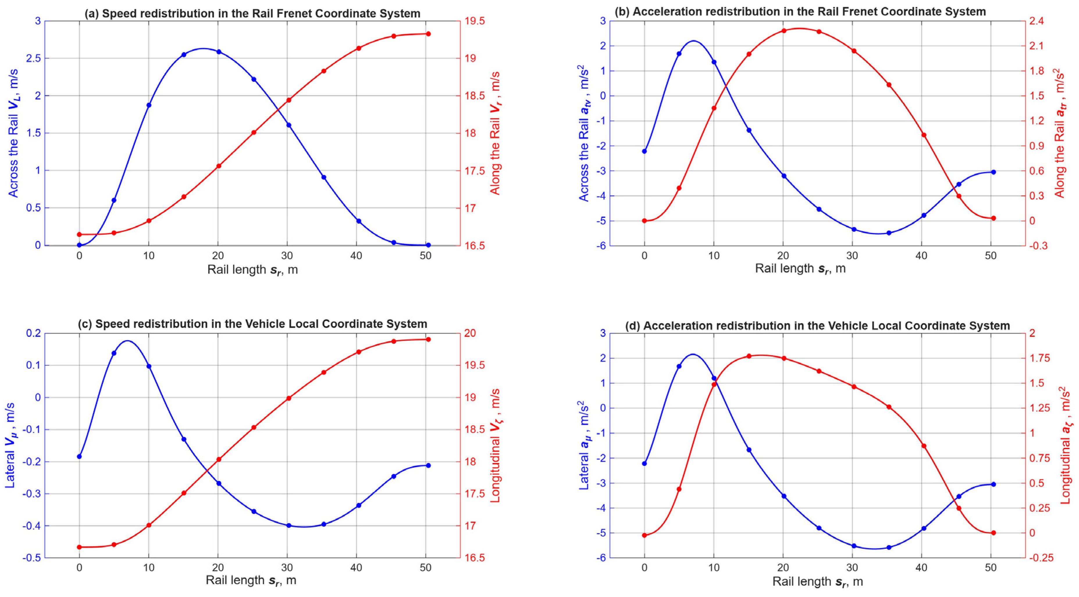
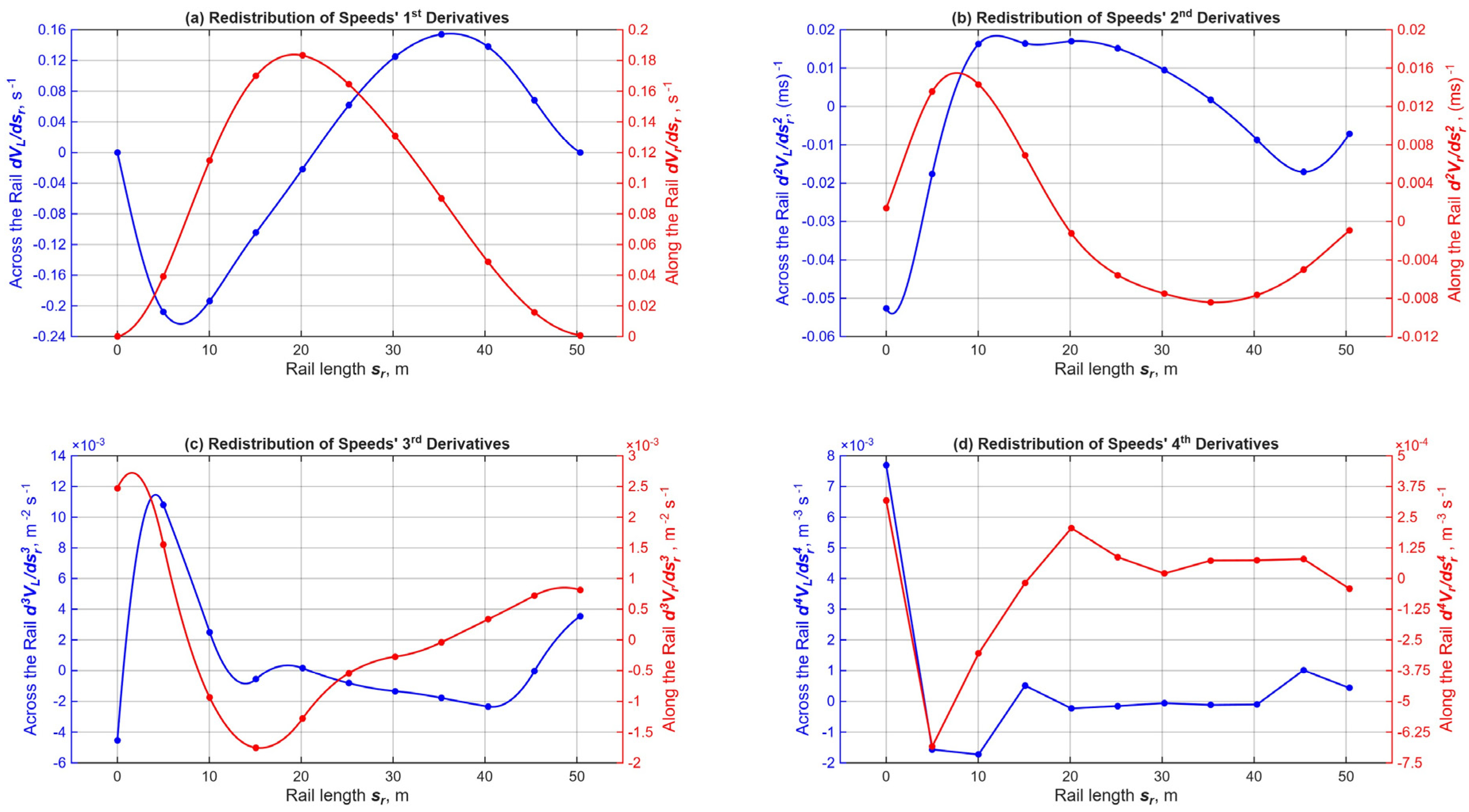
Figure 6.
Distribution of speed derivatives: (a) 1st, (b) 2nd, (c) 3rd, (d) 4th.
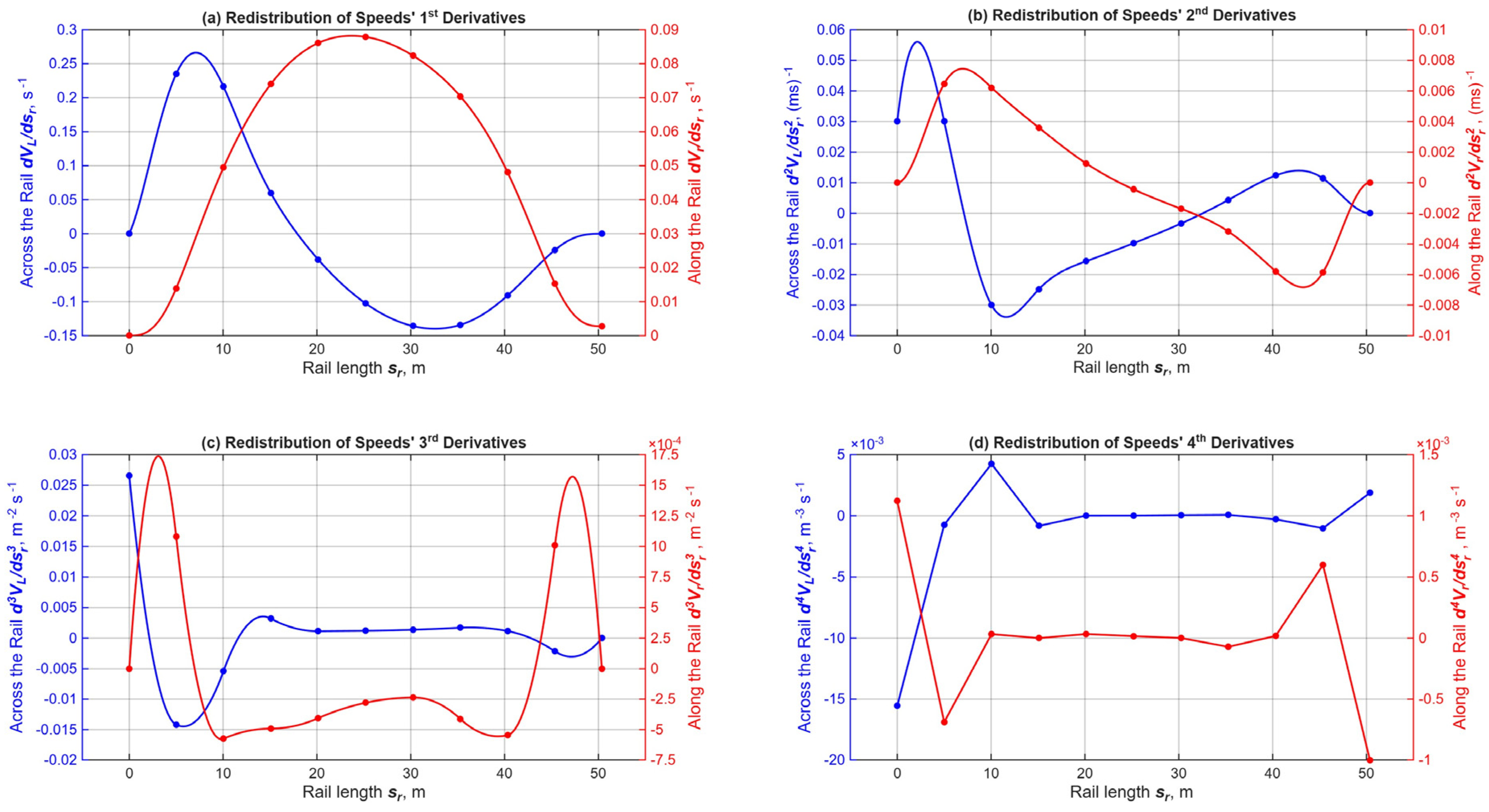
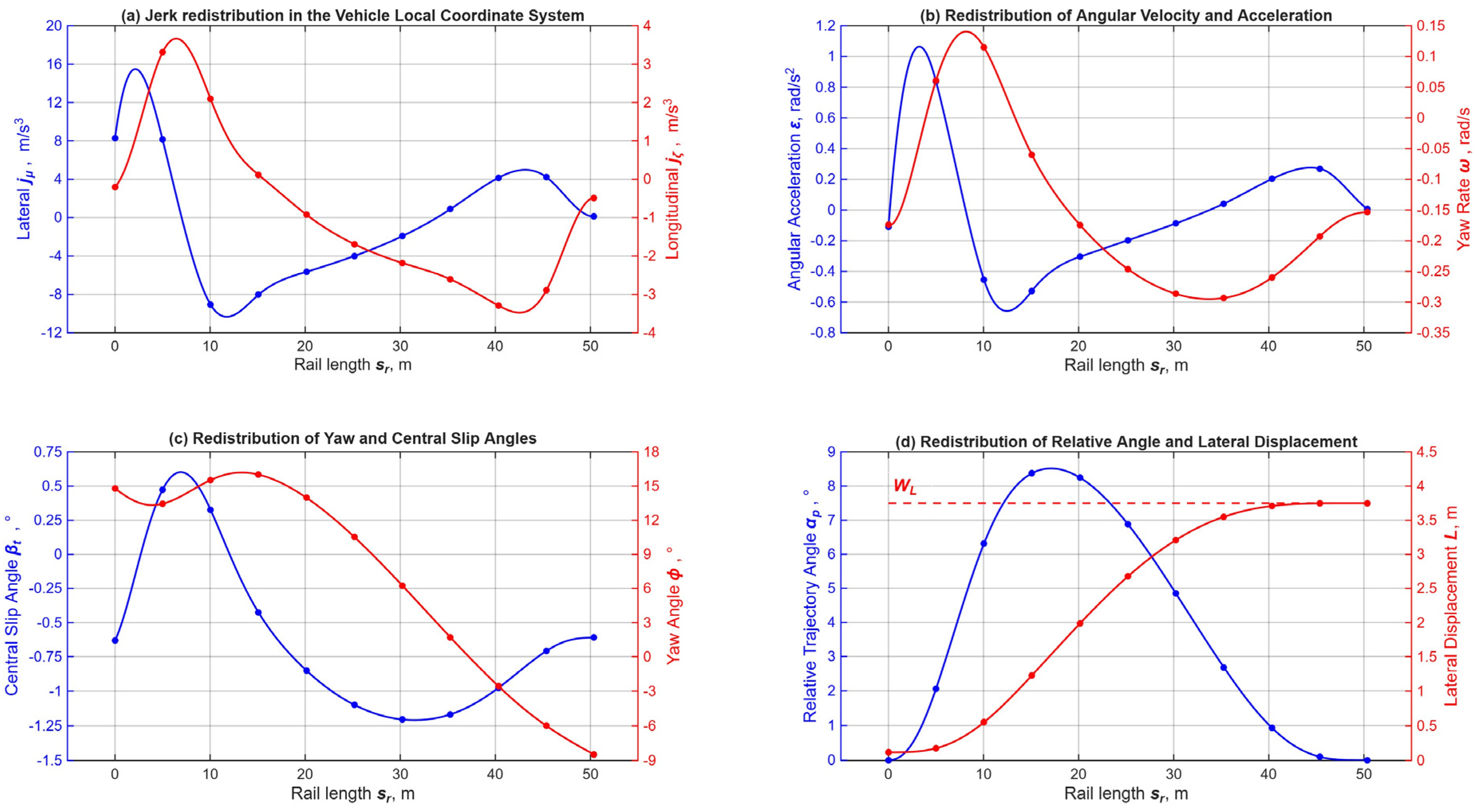
Figure 7.
Maneuver smoothness indicators: (a) jerk, (b) angular velocity and acceleration, (c) yaw and central slip angles, (d) relative trajectory angle and lateral displacement.
Figure 7.
Maneuver smoothness indicators: (a) jerk, (b) angular velocity and acceleration, (c) yaw and central slip angles, (d) relative trajectory angle and lateral displacement.
Rightward lane change.
Figure 8.
Distribution of speeds and accelerations along the rail length: (a) speeds along and across the rail, (b) accelerations in the rail coordinates, (c) speeds in the vehicle coordinate system, (d) accelerations in the vehicle coordinate system.
Figure 8.
Distribution of speeds and accelerations along the rail length: (a) speeds along and across the rail, (b) accelerations in the rail coordinates, (c) speeds in the vehicle coordinate system, (d) accelerations in the vehicle coordinate system.
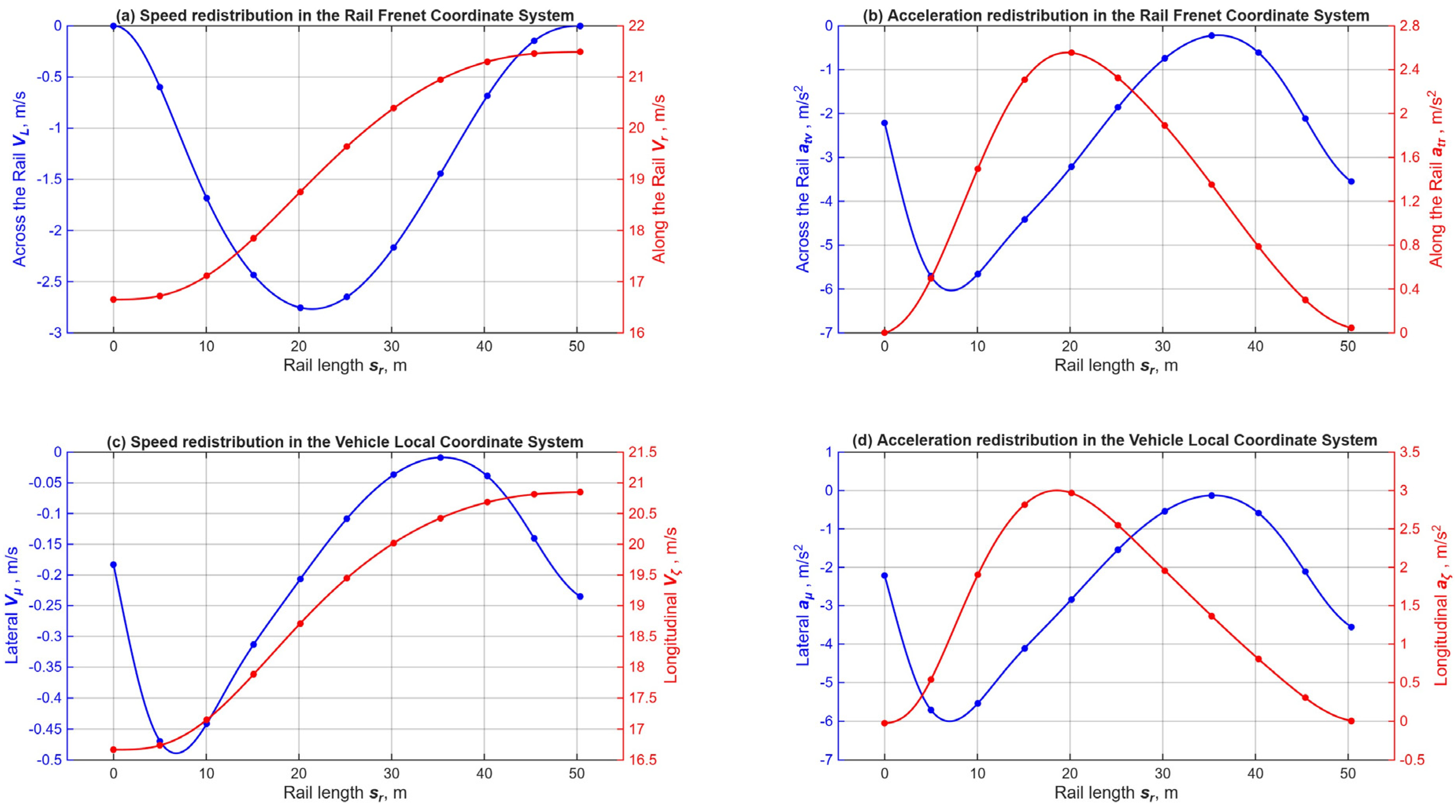
Figure 9.
Distribution of speed derivatives: (a) 1st, (b) 2nd, (c) 3rd, (d) 4th.
Analysis of Results.
Smoothness. The analysis of the obtained graphical dependencies clearly demonstrates the high smoothness of the generated plan. The curves show that the underlying manipulation of speeds and their derivatives in the longitudinal and lateral directions (along and perpendicular to the rail) ensures function continuity and eliminates abrupt jumps. Since the model is initially formulated in terms of second and third derivatives, their targeted optimization ensures that the curves in integration and differentiation plots (including combined kinematic parameters) evolve smoothly, providing inherent stability for the entire system. Minor local inflections in higher-order derivatives observed on the plots outside the knot points (like in Figure 6c, Figure 9c) are purely boundary-related - they arise exclusively from the strict enforcement of boundary conditions at the element ends. However, these effects remain localized and do not violate the overall monotonicity and predictability of the system behavior.
Continuity. The analysis of the graphs also confirms the achievement of the key effect of continuity throughout the entire trajectory structure. Even at the level of higher-order derivatives (up to the fourth), where the curves naturally lose their ideal smoothness and take on a step-like character, full continuity at the knot points is maintained without any breaks. This is achieved through boundary conditions strictly enforced during the optimization process, which require adjacent nodes to coincide, effectively «stitching» the elements together at the knot points and preventing any misalignment (Figure 6d, Figure 9d). It is here, at the level of rigorous high-order nodal alignment, that the primary stability factor of the entire system is established. If this requirement were omitted, discontinuities would inevitably propagate to lower-order levels; however, because the elements are reliably linked at the fourth derivative, the third derivative (which is directly incorporated into the basic model) is automatically rendered continuous, ensuring the predictable and stable behavior of the entire geometry.
Convergence. The analysis of the optimization process and the resulting convergence plots demonstrates high stability and predictability of the algorithm's performance. This is rooted in the model's core structure because the finite element representation based on Hermite polynomials rigorously structures the search space and analytically links parameters via nodal degrees of freedom; the nonlinear programming (SQP) task avoids excessive iterations and prevents the solver from becoming trapped in undesirable local extrema. It should be noted that at this stage, the optimizer was configured based on an assessment of factor influence, reflected through weighting coefficients; nevertheless, even with this approach, the method exhibits excellent convergence. Future research will focus on developing formalized normalization techniques and automated tuning procedures to further enhance the algorithm's efficiency and convergence speed.
Feasibility and Constraint Compliance. The analysis of the obtained graphs also confirms the full feasibility of the trajectories and the strict compliance of all parameters with the specified constraints. First, none of the curves exceed the preset limits, clearly demonstrating the effective performance of the constraints introduced into the model. Second, the parameter values on the graphs fully correspond to the capabilities of their physical implementation within the tracking loop, confirming that the vehicle can execute such trajectories without entering non-physical zones. The maneuver duration is approximately .
Low Slip Angle. The analysis of the side-slip angle distribution graphs (Figure 7c, Figure 10c) demonstrates consistently small values throughout the entire maneuver. This confirms that the motion kinematics are in strict alignment with tire dynamics: the vehicle moves without pronounced side slip, and the velocity vectors remain close to the wheels' longitudinal axis. The low slip angles indicate control stability and show that the trajectory is executed smoothly, without critical lateral loads on the tires.
Strict Final Position. The analysis of the final trajectory segments (Figure 7d, Figure 10d, Figure 11) shows that the algorithm guides the vehicle to the target point with high precision, achieving the specified final position and orientation. The absence of steady-state error at the terminal stage demonstrates the effectiveness of the boundary conditions and terminal constraints, thereby guaranteeing precise execution of the positioning task at the end of the maneuver.
7. Conclusions
This study aimed to develop an advanced mathematical framework for synthesizing a motion plan and references in a natural (curvilinear Frenet) coordinate system. Unlike classical sequential approaches that separate the search for spatial geometry and kinematics profiling into distinct stages, the proposed method implements a unified (integrated) concept. By referencing a spatial guide (virtual rail), optimization is performed simultaneously in two directions - along and across the rail. This makes it entirely possible to abandon the two-stage scheme and the rigid dependency on traffic scenarios during the geometry search phase, thereby ensuring the synchronised distribution of velocities accounting for all constraints and the generation of a comprehensive plan. Based on this study, the advantages of the proposed framework are as follows:
- Mathematical precision. Unlike other planning approaches in the natural Frenet coordinate system, the proposed method is free from simplifications, with all terms represented with high precision. The trajectory plots clearly demonstrate high smoothness in curvature variations and high accuracy of the final position. Despite the apparent complexity of the computational formulas, the optimization process is performed sufficiently fast.
- Dynamic adaptability and criterion balance. In traditional sequential schemes, priority is given to generating a maximally smooth static geometry at the initial stage, which inherently precludes lateral correction - any further adjustments are strictly limited to the longitudinal movement along the pre-fixed path. In contrast, the proposed method implements a fundamentally different paradigm: the spatial trajectory is secondary, serving merely as a result of integration, while the optimization process is centered on achieving optimal dynamics. This simultaneous generation of geometry and kinematics ensures full dynamic elasticity. Consequently, the algorithm can deliberately accept local increases in curvature to achieve superior performance in speed and time, a trade-off that is fundamentally unattainable within the constraints of rigid two-stage concepts.
- Computational performance and optimization parameters. All computational experiments were performed on a hardware platform featuring an Intel Core i7-7500U CPU @ 2.70-2.90 GHz with 8 GB of RAM. The computation time is primarily driven by the constraint set and the required solution accuracy: optimizing the virtual rail takes an average of 0.5 s, while generating the motion plan ranges from 0.5 to 2.4 s. Optimization was carried out using the fmincon solver via the sequential quadratic programming (SQP) algorithm with finite difference gradient approximation. For the rail optimization, the optimality, constraint, and step tolerances were all set to . For the motion plan generation, the precision was increased by two orders of magnitude with all tolerances set to , and the maximum number of iterations was capped at 250 (note that convergence is successfully achieved with as few as 50 iterations yielding identical results).
- Mesh and integration point variability. Algorithm performance can be flexibly adjusted over a wide range by varying the number of finite elements and employing Gauss integration schemes with 2 to 8 points. Notably, solution quality is not always strictly proportional to the number of nodes, allowing for an effective trade-off between accuracy and computational speed.
- Constraint flexibility. The proposed framework incorporates numerous constraint factors that can be selectively deactivated to improve computational speed, particularly when handling coupled constraints such as the terminal angle and terminal path curvature.
- Segment matching accuracy. Although this study focuses on a single road segment, the optimized output parameters enable seamless concatenation with subsequent sections. By using the terminal parameters of higher-order derivatives from the current plan as initial conditions for the next plan, trajectory smoothness is automatically guaranteed, even for compound parameters such as jerks.
- Mathematical complexity and fixed rail horizon. Deriving the mathematical framework requires high precision and rigorous multi-stage verification; however, this effort is fully compensated by the quality and speed of prediction. At the current stage, the length of the virtual rail remains fixed (non-telescopic). Consequently, the system is constrained in its ability to adaptively shorten or extend the base trajectory horizon depending on external factors - such as the presence of static and dynamic obstacles (which require real-time horizon adjustments for safe maneuvering) and the tire-road friction coefficient (where low adhesion or safety constraints regarding lead vehicles necessitate a flexible rail length).
While this study establishes the fundamental mathematical framework and simultaneous optimization architecture for advanced Frenet-based motion planning, it opens several promising avenues for future research within this series:
- Comparative Analysis of 2-DOF and 3-DOF Dynamic Models: Future work will extend the framework to a vehicle dynamic model with three degrees of freedom utilizing fifth-degree Hermite polynomials. Although a 3-DOF model introduces more optimization parameters, the increased structural elasticity is expected to permit a significantly reduced number of nodal points, and a dedicated comparative study will evaluate the performance trade-offs between the two formulations.
- Optimization Robustness and Guaranteed Convergence: A rigorous investigation will be conducted to ensure that the proposed optimization process executes within a strictly bounded, finite time and yields predictable results across arbitrary initial conditions, guaranteeing deterministic performance under all operational scenarios.
- Comprehensive Constraint Integration: Upcoming studies will incorporate a much broader spectrum of constraints omitted in the current baseline—specifically focusing on spatial restrictions imposed by static and dynamic obstacles, as well as physical limitations such as tire-road friction boundaries.
- Seamless Multi-Segment Stitching and Lane Change Transitions: Future developments will feature extensive experimentation on managing transient processes during sequential segment stitching. Since the virtual rail and spline are regenerated for each new lane after a maneuver, upcoming work will mathematically and experimentally validate the curvature transition formulas to ensure smooth spatial and temporal continuity across successive planning horizons.
Author Contributions
Conceptualization, MD and SME; methodology, MD; software, MD; validation, MD and SME; formal analysis, MD and SME; investigation, MD; resources, SME; data curation, MD; writing - original draft preparation, MD and SME; writing - review and editing, MD and SME; visualization, MD; supervision, SME; project administration, SME; funding acquisition, SME All authors have read and agreed to the published version of the manuscript.
Funding
This research is financially supported by the Natural Sciences and Engineering Research Council of Canada (grant No. RGPIN-2020-04667).
Institutional Review Board Statement
No institutional review is required.
Informed Consent Statement
Not applicable.
Data Availability Statement
Some or all data, models, or codes that support the findings of this study are available from the corresponding author upon reasonable request.
Conflicts of Interest
The authors declare no conflicts of interest.
References
- Song, X.; Gao, H.; Ding, T.; Gu, Y.; Liu, J.; Tian, K. A review of the motion planning and control methods for automated vehicles. Sensors 2023, 23(13), 6140. [Google Scholar] [CrossRef] [PubMed]
- Teng, S.; Hu, X.; Deng, P.; Li, B.; Li, Y.; Ai, Y.; Yang, D.; Li, L.; Xuanyuan, Z.; Zhu, F.; Chen, L. Motion planning for autonomous driving: The state of the art and future perspectives. IEEE Trans. Intell. Veh. 2023, 8(6), 3692–3711. [Google Scholar] [CrossRef]
- Tariq, F.M.; Yeh, Z.-H.; Singh, A.; Isele, D.; Bae, S. Frenet Corridor Planner: An optimal local path planning framework for autonomous driving. 2025 IEEE 36th Intelligent Vehicles Symposium (IV), 2025; pp. 1–8. [Google Scholar] [CrossRef]
- Muzzini, F.; Capodieci, N.; Ramanzin, F.; Burgio, P. GPU implementation of the Frenet Path Planner for embedded autonomous systems: A case study in the F1tenth scenario. J. Syst. Archit. 2024, 154, 103239. [Google Scholar] [CrossRef]
- Dang, B.; Chen, H.; Zhang, H.; Wang, J.; Zhou, J. Intelligent vehicle lane-changing strategy through polynomial and game theory. Comput. Mater. Contin. 2025, 83(2), 2003–2023. [Google Scholar] [CrossRef]
- Wang, T.; Qu, D.; Wang, K.; Wei, C.; Li, A. Risk-aware lane change and trajectory planning for connected autonomous vehicles based on a potential field model. World Electr. Veh. J. 2024, 15(11), 489. [Google Scholar] [CrossRef]
- Hu, C.; Huang, J.; Mao, W.; Xie, L. FSDP: Fast and safe data-driven overtaking trajectory planning for head-to-head autonomous racing competitions. 2025 IEEE/RSJ International Conference on Intelligent Robots and Systems (IROS), 2025; pp. 1–8. [Google Scholar] [CrossRef]
- Diachuk, M.; Easa, S.M. Simultaneous trajectory and speed planning for autonomous vehicles considering maneuver variants. Appl. Sci. 2024, 14(4), 1579. [Google Scholar] [CrossRef]
- Zhang, X.; Zang, Z.; Song, J.; Qi, J.; Gong, J. Efficient path–velocity coupled trajectory planning for autonomous vehicles using sparse normal plane constrained trajectories. Adv. Eng. Inform. 2025, 70, 104236. [Google Scholar] [CrossRef]
- Easa, S.M.; Diachuk, M. Inverse dynamics-based motion planning for autonomous vehicles: Simultaneous trajectory and speed optimization with kinematic continuity. World Electr. Veh. J. 2025, 16(5), 272. [Google Scholar] [CrossRef]
- Hung, N.; Rego, F.; Quintas, J.; Cruz, J.; Jacinto; Potes, A. A review of path following control strategies for autonomous robotic vehicles: theory, simulations, and experiments; 2022. [Google Scholar]
- Zhou, H.; Liu, J. RDT-RRT: Real-time double-tree rapidly-exploring random tree path planning for autonomous vehicles. ACM Trans. Intell. Syst. Technol. 2024, 15(3), 1–22. [Google Scholar] [CrossRef]
- Hu, J.; Chang, Y.-C.; Wang, H. A review of learning-based motion planning: Toward a data-driven optimal control approach. arXiv 2025b. [Google Scholar]
- Werling, M.; Ziegler, J.; Kammel, S.; Thrun, S. Optimal trajectory generation for dynamic street scenarios in a Frenét Frame. 2010 IEEE International Conference on Robotics and Automation, 2010; pp. 987–993. [Google Scholar]
- Peng, B.; Yu, D.; Zhou, H.; Xiao, X.; Xie, C. A motion planning method for automated vehicles in dynamic traffic scenarios. In Symmetry; 2022. [Google Scholar] [CrossRef]
- Huang. Trajectory planning in Frenet frame via multi-objective optimization. IEEE Access 2023, 11, 70764. [Google Scholar] [CrossRef]
- Deolasee, S.; Lin, Q.; Li, J.; Dolan, J.M. Spatio-temporal motion planning for autonomous vehicles with trapezoidal prism corridors and Bezier curves. In Proceedings of the 2023 American Control Conference (ACC), San Diego, CA, USA, 2023. [Google Scholar]
- Wang. Research on path planning for autonomous vehicle based on Frenet system. J. Eng. Res. 2023, 11, 100080. [Google Scholar] [CrossRef]
- Li, B.; Zhang, Y. (202 Fast trajectory planning in Cartesian rather than Frenet frame: A precise solution for autonomous driving in complex urban scenarios. IFAC Pap. 53, 17065. [CrossRef]
- Gu, T.; Dolan, J.M. On-road motion planning for autonomous vehicles. In Proceedings of the International Conference on Intelligent Robotics and Applications, Montreal, QC, Canada, 2012. [Google Scholar] [CrossRef]
Figure 1.
Schematic representation of the AV trajectory generation within the reference Frenet coordinate system.
Figure 1.
Schematic representation of the AV trajectory generation within the reference Frenet coordinate system.
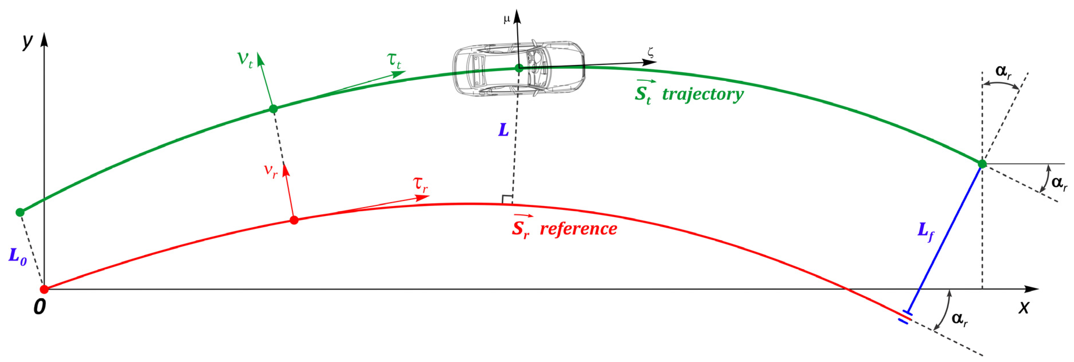
Figure 2.
Geometric scheme for trajectory composition within the reference Frenet frame: (a) fundamental differential geometric relationships; (b) chord approximation of the arc element.
Figure 2.
Geometric scheme for trajectory composition within the reference Frenet frame: (a) fundamental differential geometric relationships; (b) chord approximation of the arc element.
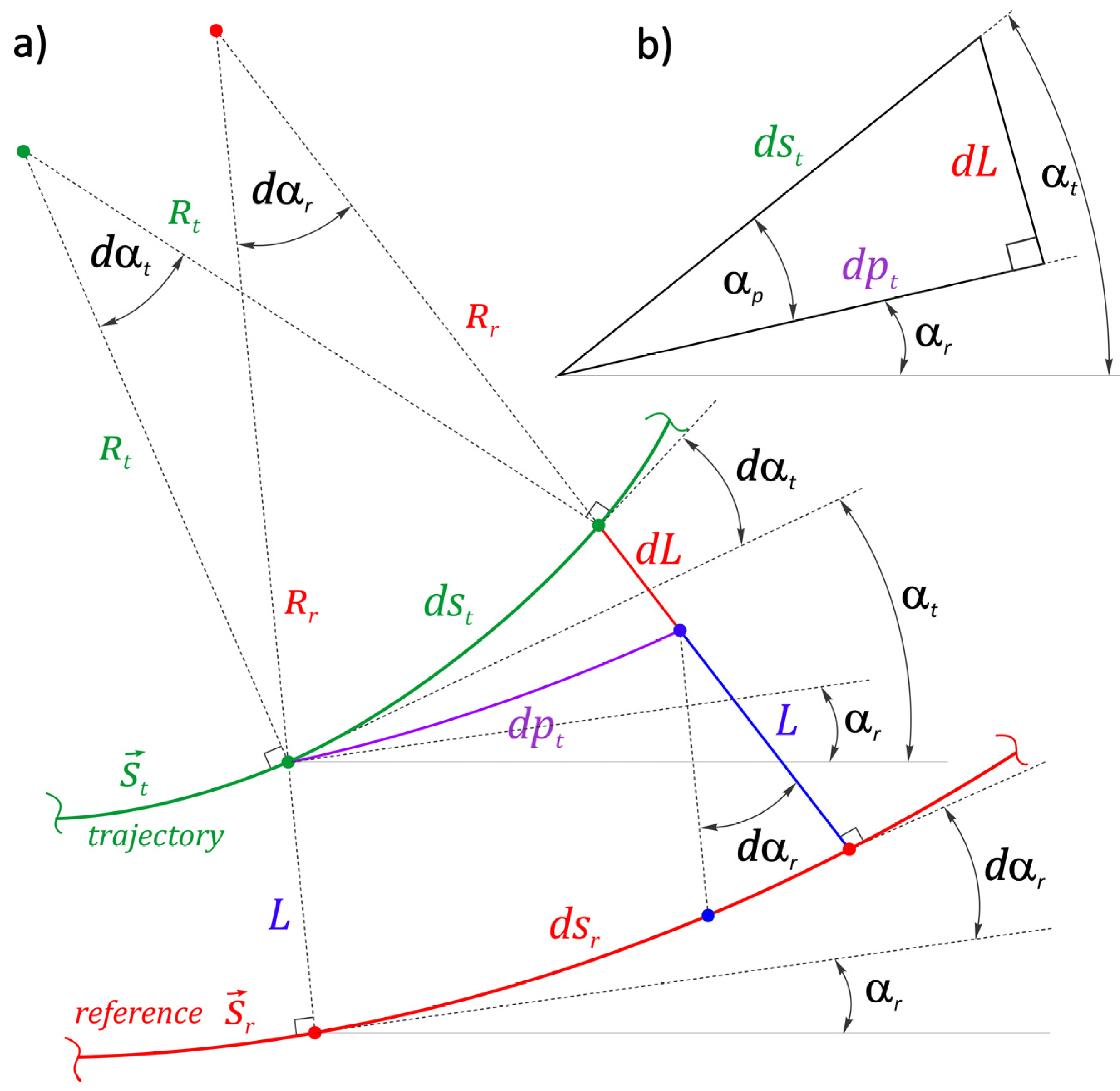
Figure 3.
Scheme of a curved road section with options for lane change.
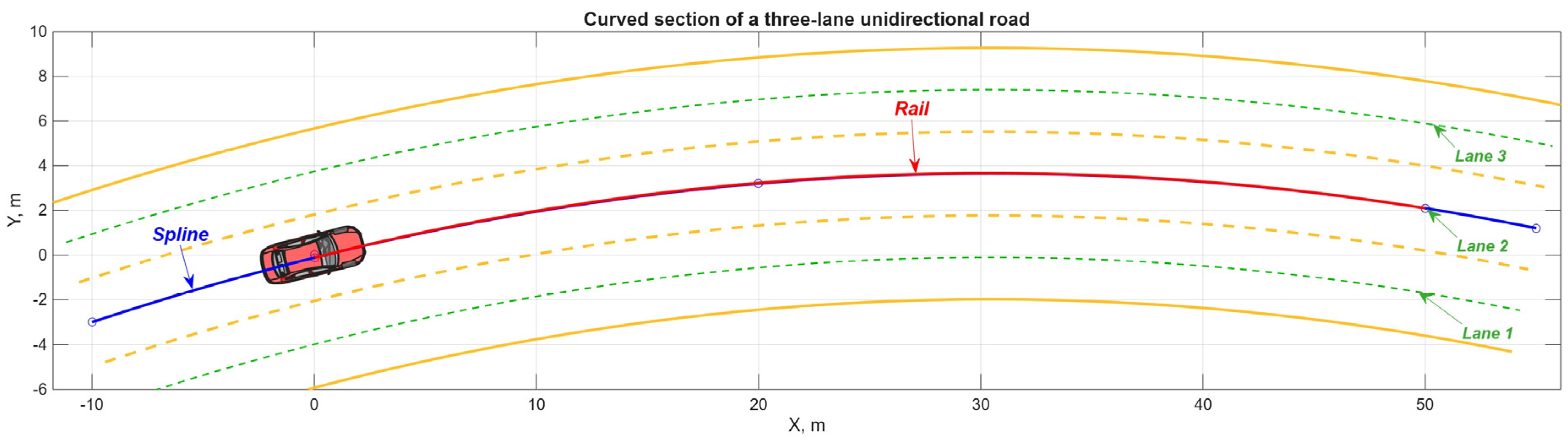
Figure 4.
Optimization results for the virtual rail model: (a) angular parameters and matching error; (b) curvature profile and its first rate of change; (c) second and third curvature derivatives; (d) higher-order (fourth and fifth) curvature derivatives.
Figure 4.
Optimization results for the virtual rail model: (a) angular parameters and matching error; (b) curvature profile and its first rate of change; (c) second and third curvature derivatives; (d) higher-order (fourth and fifth) curvature derivatives.
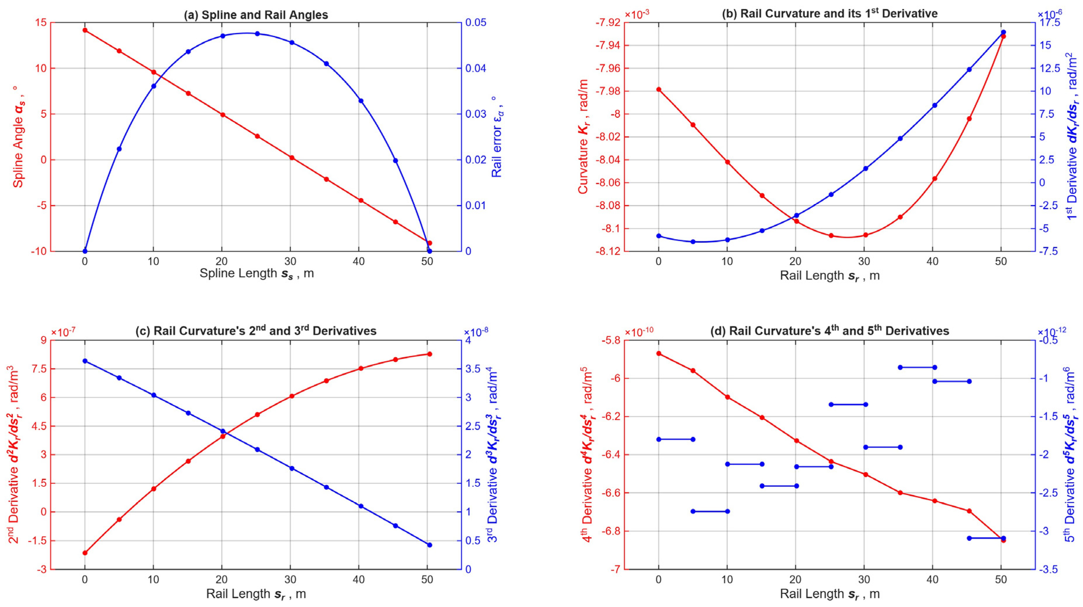
Figure 10.
Maneuver smoothness indicators: (a) jerk, (b) angular velocity and acceleration, (c) yaw and central slip angles, (d) relative trajectory angle and lateral displacement.
Figure 10.
Maneuver smoothness indicators: (a) jerk, (b) angular velocity and acceleration, (c) yaw and central slip angles, (d) relative trajectory angle and lateral displacement.
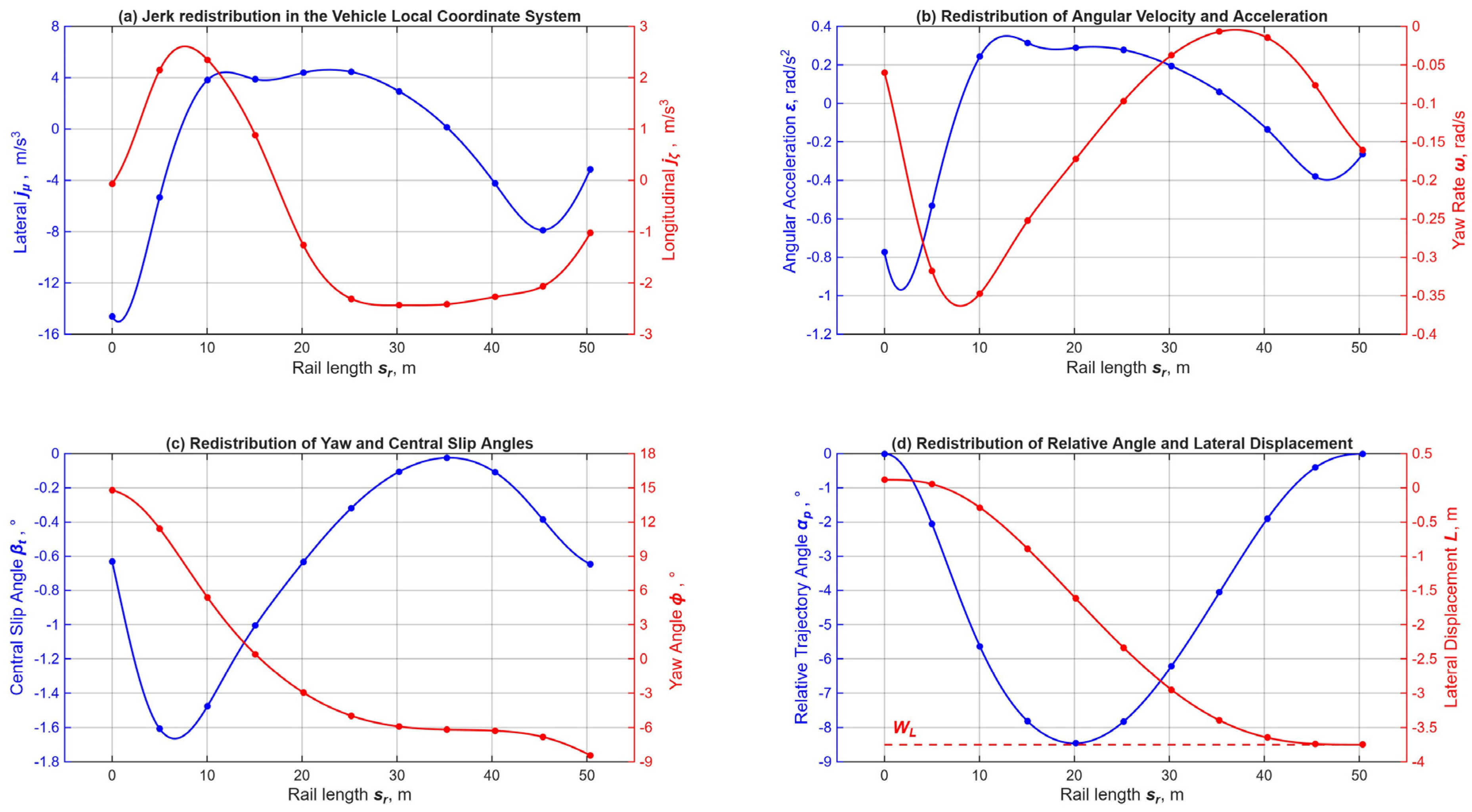
Figure 11.
Variants of predicted maneuver trajectories on a 3-lane road.
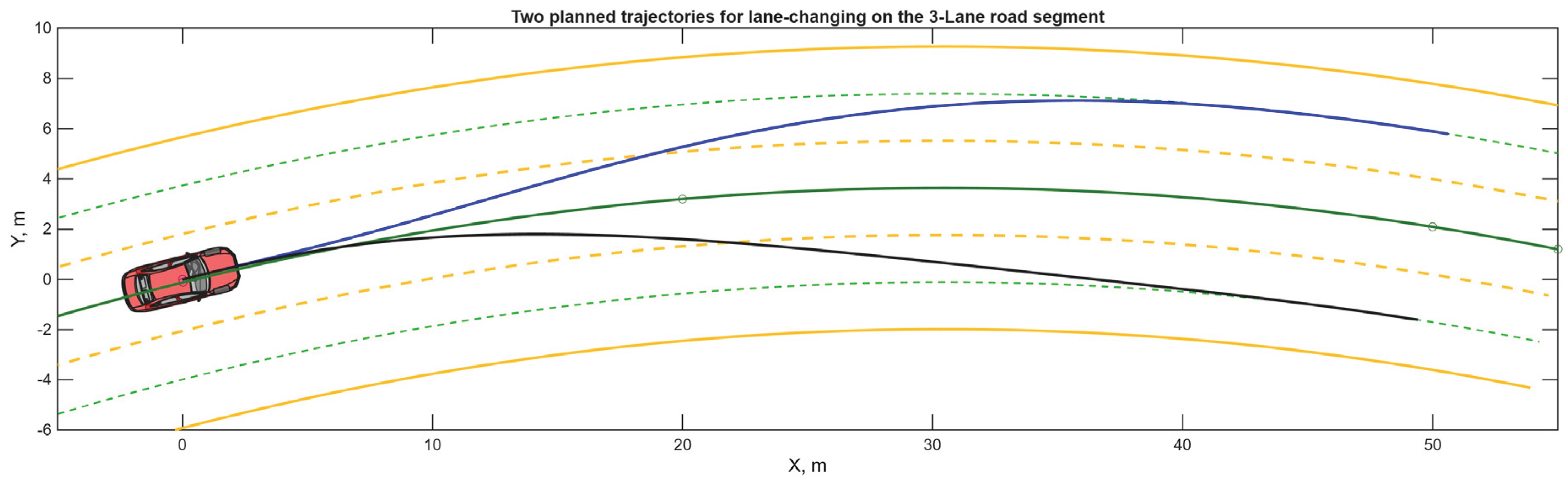
Disclaimer/Publisher’s Note: The statements, opinions and data contained in all publications are solely those of the individual author(s) and contributor(s) and not of MDPI and/or the editor(s). MDPI and/or the editor(s) disclaim responsibility for any injury to people or property resulting from any ideas, methods, instructions or products referred to in the content. |
© 2026 by the authors. Licensee MDPI, Basel, Switzerland. This article is an open access article distributed under the terms and conditions of the Creative Commons Attribution (CC BY) license (http://creativecommons.org/licenses/by/4.0/).
Copyright: This open access article is published under a Creative Commons CC BY 4.0 license, which permit the free download, distribution, and reuse, provided that the author and preprint are cited in any reuse.