

Submitted:
11 September 2026
Posted:
14 September 2026
You are already at the latest version
Abstract
Discharge schemes in particle models of thunderclouds remove charge from a stochastically grown channel, which does not conserve charge and imposes the channel geometry rather than deriving it. This paper replaces the scheme with a plasma process: when the field in the gap between two oppositely signed charge layers reaches the ionization level the gap is filled with neutral air at the simulation’s own initial density, molecules above threshold separate into a positive ion and an electron, and everything after that follows from the force law that moves every other particle. Charge is conserved at every reaction. Two quantities such schemes leave free are derived rather than chosen: the separation at which a new pair is unbound, from the ambient field, and the timestep, from the electron drift velocity at the reduced field the model itself produces, E/N = 27 Td. In a column whose charge layers are prescribed rather than generated, the same charge spread smoothly through each layer gives 19 kV m⁻¹ and never fires; gathered into local concentrations it gives up to 196 kV m⁻¹ and does. The requirement is a layered and locally concentrated charge structure. Rotation is how this model produces one, but the discharge acts identically on prescribed layers that no vortex has shaped. Against matched controls the field in the firing gap falls 55.8 ± 6.5 per cent over eleven seeds, with relief of neighbouring gaps attenuating to zero by 2.16 km. Without an electron attachment loss the discharge never terminates; with attachment on oxygen all ten discharges self-terminate, at a median 190 ms and 1.44 × 10⁴ m s⁻¹ against 192 ms and 1.69 × 10⁴ m s⁻¹ for flashes measured in a mapped storm using the model’s own definitions. The reach is a factor of four short, which bounds the result to initiation and local field relief rather than to flash extent. Two predictions follow that observation can test: initiation should track the concentration of charge within a layer rather than the layer-averaged field, and flash duration should scale with the oxygen number density that sets the attachment length.
Keywords:
thundercloud electrification
; gap-ionization discharge
; particle model
1. Introduction
Balloon soundings through convective regions do not find a simple dipole. They find several thin layers of alternating polarity, four inside updrafts and at least six outside them, individual layers often a few hundred metres thick (Williams, 1989; Stolzenburg et al., 1998). That fine structure, rather than any storm-scale potential difference, is what a discharge encounters: it is the local field between adjacent layers that first exceeds breakdown. How a discharge behaves in such a structure is a question about the gaps between layers, and it is the question this paper addresses.
Particle models of electrified clouds generally discharge by the stochastic dielectric-breakdown scheme of Niemeyer et al. (1984), developed for thunderclouds by Mansell et al. (2002): a channel is grown cell by cell through a solved field, and the charge inside it is then set to zero. That scheme has a defect. It destroys charge. A carrier inside the channel has its charge removed irrespective of sign and with no counterpart anywhere in the domain, so the net charge of the column changes by whatever the channel happened to contain. Real lightning conserves charge: a bidirectional leader is a conductor that moves negative charge one way and positive the other and deposits it at the channel ends (Kasemir, 1960). The consequence is not cosmetic. Because deletion lowers the field everywhere, a discharge in such a scheme can never raise the field anywhere, and the refractory timing reported in the first paper is therefore partly a property of the scheme rather than a discovery about the storm.
This paper replaces that scheme rather than patching it. The replacement is a plasma process with no channel in it. When the axial field between two oppositely signed layers reaches the ionization level, the space between them is filled with neutral air, molecules sitting where the local field is strong enough are separated into an ion and an electron, and from that point everything is the same force law that moves every other particle in the model. There is no propagation rule, no branching exponent, no neutralisation fraction and no Poisson grid. The discharge is whatever the ionized air does.
Three consequences follow, and they organise the paper. Charge is conserved exactly, so the objection above is answered. Two quantities that look like free parameters turn out to be derivable, which removes them from the list of things a reader must take on trust. And because the model now contains electrons with a physical mass ratio moving under a clock that can be anchored to laboratory swarm data, the speed at which the ionization front advances becomes an output rather than an input – a quantity the model predicts and observation can refute.
The mechanism under examination was proposed as a physical chain: rotation sorts charge into layers; the field between layers grows; that field ionizes the air between them; the electrons released near a negative layer accelerate toward the positive one; some survive the crossing, are re-accelerated on the far side, and ionize further. Each link is examined here in turn, and the last two – the crossing and the subsequent ionization – are measured per particle rather than inferred.
The contribution is fourfold. First, a discharge scheme for particle models of electrified clouds that conserves charge exactly, imposes no channel and requires no propagation rule, no Poisson grid and no breakdown lattice: the entire discharge follows from the same force law that moves every other particle in the domain. Second, the removal of two quantities that such schemes normally leave free. The separation at which a newly created pair is unbound is derived here from the ambient field rather than chosen, and the timestep is anchored on the electron drift velocity at the reduced field the model itself produces, which converts the propagation speed from a tuned quantity into a falsifiable output. Third, a statement of what the mechanism actually requires of a charge structure, established by building the structure by hand rather than inferring it from the model that generated it: layering alone is not sufficient, and local concentration within the layers is necessary. Fourth, a quantitative test against mapped flashes in which the observations are reduced with the model’s own definitions rather than taken from published summary statistics, reporting both the two quantities that agree without having been fitted and the one that does not.
What the paper does not claim should be stated with the same precision. It does not claim that this mechanism produces lightning, and it does not exclude that it does. What is demonstrated is narrower than the first and stronger than nothing. It demonstrates that a mechanism assembled from the rules above produces localised, subcritical, charge-transferring discharges whose duration, propagation speed and charge moment fall within observed ranges, and it identifies precisely where the resemblance fails. The distinction matters because the charging model beneath the discharge has documented deficiencies, set out in Sect. 10, that no discharge treatment can repair.
One objection to that model is answered here rather than conceded, and it is worth flagging at the outset because it determines how much of the paper survives the objection. If the layered charge structure the discharge acts on were an artefact of vortex sorting – of a charging model with no gravity, no size spectrum and no fall speeds – then nothing measured downstream of it would mean anything. Section 4 removes the question by building the layers by hand, in a column no vortex has ever acted on, and running the identical discharge on them. The discharge does not care how the layers arrived. What it requires of them is stated there and is narrower and more useful than a rotating column: layering together with local concentration within the layers.
2. The Model
The model described here is Thunder v1.0. It comprises a charging component, which produces a layered charge structure in a rotating particle column, and the discharge component that is the subject of this paper. The two are separable: Sect. 4 shows that the discharge acts on any layered and locally concentrated charge structure, including one assembled by hand, and does not depend on how the charging component produced it. Both components, together with every script used below, are archived as described in the code and data availability section.
2.1. The Charging Model
The column is a minimal particle model, specified here in full. Carriers of unit mass move under a prescribed Rankine vortex with a conical envelope and a Gaussian axial weighting, feel a pairwise Coulomb and Biot–Savart force within a cutoff, and exchange charge on contact: two neutrals in contact separate as a positive and a negative, and two opposite charges in contact neutralise, each with a refractory period afterwards. There is no microphysics, no size spectrum and no sedimentation. Table 1 lists every constant.
2.2. What the Discharge Acts on
Left to run, the column organises into an annulus with an evacuated core, and within that annulus the charge separates into axial layers of alternating sign. Figure 1 shows the state to which the discharge scheme is applied. Two features of it matter, and they are separable.
The first feature is the layering, visible in panel (b) as alternating bands. The second is the fine structure within each layer, visible in panel (a): the carriers are not spread smoothly but gathered into dense filaments a few hundred metres across. Section 4 shows that the second, not the first, is what produces a field able to ionize anything.
2.3. The Column
Three quantities fix the column in physical units. One model unit is 40 m. The column occupies 6 to 10.8 km in height and an annulus of roughly 2 to 4.5 km radius. Charge is anchored by matching the densest axial layer to an observed convective layer density of 1 nC m⁻³, which fixes the carrier charge at 0.349 C for the 30,000-carrier configuration used throughout.
A settled column develops alternating axial layers. The gaps between consecutive layers of opposite sign are what the discharge scheme acts on, and they are located from the axial net-charge profile rather than specified: a layer is a local extremum reaching 30 per cent of the largest excursion, and a gap is the span between two consecutive extrema of opposite sign.
2.4. Species and Masses
Three populations are present. The hydrometeor carriers are those of the charging model. When a discharge begins, two further species appear: neutral air molecules, and the ions and electrons they produce. The two kinds of particle are never interchanged. A carrier acquires charge only by contact with another carrier and is never ionized; an air molecule is never charged by contact and enters only through ionization. The threshold of Sect. 2.9 is accordingly the field at which air ionizes, not a field at which a hydrometeor loses an electron.
Carrying only hydrometeors until that threshold is reached is a physical statement rather than a simplification of convenience. The charge that builds the layered structure resides on hydrometeors, deposited by rebounding graupel–crystal collisions in the mixed-phase region (Takahashi, 1978; Saunders et al., 2006). Air is present throughout, but while that structure forms it is electrically close to passive: background conductivity inside a thundercloud is of order 10⁻¹⁴ S m⁻¹ or less, below that of clear air at the same altitude because small ions attach to hydrometeors and the charge they carry is immobilised (MacGorman and Rust, 1998; Iudin et al., 2019). The Maxwell relaxation time ε₀/σ that follows from that conductivity is of order 10³ s, long compared with the interval over which the layers assemble, so conduction through the air does not materially relax the structure while it is being built. Air becomes electrically active in one circumstance, when the field between two layers reaches the ionization level, and the model introduces it at exactly that point. What this leaves out is the weak conduction current itself and the screening layers it forms at cloud boundaries, both of which act on the large-scale charge distribution rather than on the gap between two adjacent layers.
Air at 77 per cent N₂ and 23 per cent O₂ has a mean molar mass of 0.77 × 28.013 + 0.23 × 31.998 = 28.93 g mol⁻¹, within 0.1 per cent of the 28.96 g mol⁻¹ of real dry air. An electron is 5.486 × 10⁻⁴ g mol⁻¹, so
and that ratio is used exactly. It is not a mobility parameter. The transport asymmetry reported in Sect. 6.3, in which electrons travel some 200 times further than ions over the same interval in the same field, follows from it rather than being imposed alongside it.
m_e / m_atom = 1.897 × 10⁻⁵,
The mass of an air particle relative to a hydrometeor is not a physical constant, because both are coarse-grained parcels rather than single objects, and it is therefore exposed as a parameter. Its value is examined in Sect. 8.

Table 3.
Species and their masses. Only the electron-to-atom ratio is a physical constant; the atom-to-hydrometeor ratio is a coarse-graining choice, because both are parcels rather than single objects.
Table 3.
Species and their masses. Only the electron-to-atom ratio is a physical constant; the atom-to-hydrometeor ratio is a coarse-graining choice, because both are parcels rather than single objects.
| Species | Mass | Basis |
|---|---|---|
| Hydrometeor carrier | 1 (reference) | Charging model of Paper I |
| Air molecule | 0.05 | Parameter; swept in Sect. 7 |
| Positive ion | 0.05 | Same as the parent molecule |
| Electron | 9.48 × 10⁻⁷ | 1.897 × 10⁻⁵ of the molecule, exact |
2.5. Reactions
Five reactions are implemented. Every one of them conserves charge, and this is asserted in code at each event rather than assumed.
Table 4.
The reaction set. The particle counts on the right are what distinguishes this scheme from one that deletes charge: nothing is removed except in pairs, and impact ionization produces three particles from two while leaving the incident electron’s identity intact.
Table 4.
The reaction set. The particle counts on the right are what distinguishes this scheme from one that deletes charge: nothing is removed except in pairs, and impact ionization produces three particles from two while leaving the incident electron’s identity intact.
| Reaction | Products | Count |
|---|---|---|
| Field ionization | atom → ion⁺ + e⁻ | 2 from 1 |
| Impact ionization | e⁻ + atom → ion⁺ + 2 e⁻ | 3 from 2 |
| Recombination | e⁻ + ion⁺ → atom | 1 from 2 |
| Hydrometeor capture | e⁻ + hydrometeor⁺ → hydrometeor⁰ | 1 from 2 |
| Elastic reflection | e⁻ + hydrometeor⁻ → reflected | no change |
Impact ionization costs the incident electron the ionization energy, applied as a kinetic-energy subtraction v′ = √(v² − v_ion²). An electron slower than v_ion cannot ionize. This is the Townsend threshold expressed as an energy condition rather than as a probability, and it is what stops an avalanche when the field can no longer re-accelerate electrons between collisions.
Electron–neutral scattering is treated as a continuum rather than against the sampled molecules, and the split is deliberate. Real air holds of order 10²⁵ molecules per cubic metre; the molecules tracked here are a sparse sample of it, so the true elastic and excitation collision rates have nothing to do with how many sample molecules happen to be nearby. Ionization is tracked discretely because it changes the charge state of a tracked particle; scattering does not. Elastic collisions cost an electron only 2m_e/M ≈ 3.8 × 10⁻⁵ of its energy and therefore randomise direction; inelastic excitation of N₂ removes energy and is where most of an electron’s energy goes in air, fixing the drift velocity and with it the effective ionization coefficient.
The approximation this makes should be stated rather than left implicit: the electron energy distribution is governed by the real gas density, while the events that change a particle’s charge state are sampled from the tracked subset. The two are consistent so long as the tracked molecules are sparse relative to the real gas, which is the regime the model occupies by construction and by four orders of magnitude at the fills used here. It would break down in the opposite limit, where the tracked sample approached the real density and the same collision would be counted twice – once in the continuum rate and once discretely. Nothing in the runs reported here comes near that limit.
Attachment is on oxygen and not on nitrogen, for a reason worth stating because it is the same asymmetry that governs the positive ions. O₂ has a positive electron affinity of 0.45 eV, so O₂⁻ is bound; N₂ has a negative affinity near −1.9 eV and forms only a shape resonance around 2.3 eV with a lifetime of order 10⁻¹⁴ s, which decays back to N₂ and a free electron. Nitrogen takes energy and returns the electron; oxygen takes the electron. On the positive side, ionization produces mostly N₂⁺ by abundance, but it charge-transfers to O₂⁺ within nanoseconds because O₂ has the lower ionization potential (12.07 against 15.58 eV), and clusters thereafter. A single positive species at the mean air mass is therefore an adequate coarse-graining, and the model is slightly optimistic about ion mobility because the terminal cluster ions are heavier.
2.6. The Pair Separation Is Derived, Not Chosen
When a molecule ionizes, the ion and the electron must be placed. Placing them at the same point is wrong in a way that is easy to miss: the pair is then bound. Its own mutual Coulomb field exceeds the ambient field, the electron is drawn back, and no free charge results. In the first implementation a fixed offset of 60 m was used, at which the pair’s mutual field is 0.111 in model units against an ambient 0.058; every pair was bound, the products accelerated into one another and left the domain at a 15 km spread.
The correct separation follows from equating the two. Setting the pair’s mutual field equal to the ambient,
in model units with unit carrier charge. Below this the split does nothing; above it the ambient field wins and the products separate. Evaluated at the measured gap fields this returns 118 to 147 m consistently across every run. It is the coarse-grained analogue of Onsager field-assisted dissociation: in real air the Coulomb binding of an electron–ion pair is overcome at Ångström scale by thermal energy and the ambient field, but a carrier here represents some 10¹⁰ hydrometeors’ worth of charge, so the same balance moves out to tens or hundreds of metres. The separation is fixed by the carrier charge and the local field, and is therefore a prediction of the coarse-graining rather than a choice.
q / (2d)² = E ⟹ d = 1 / (2√E),
2.7. Softening of the Coulomb Force
A carrier is not a point. Anchored to 1 nC m⁻³ it stands for roughly 0.35 C, and treating that as a point charge is wrong at separations below the parcel size. Unsoftened, the near field of the nearest neighbour swamps the collective field of the charge layers. Measured on a settled column, an electron takes steps of order 128 m under the local field but nets only about 100 m over 24 iterations: the coherent axial component is roughly 3 per cent of what it feels, and products scatter rather than drift.
Plummer softening at the mean inter-carrier spacing removes the spurious near field and leaves the structure. This is standard practice in N-body work for exactly this reason. The softening length used throughout is 6 model units (240 m) against a measured carrier spacing of 244 to 291 m. Section 8 reports the sensitivity.
2.8. The Sub-Clock and Its Anchor
Electrons in air drift at 10⁴ to 10⁵ m s⁻¹. One model unit is 40 m and one host iteration is about 24 s of real time, so an electron would cross the 16 km domain many times within a single host step; it cannot be integrated on the host clock at all. The air species therefore runs on its own timestep while the hydrometeors are held still. That is operator splitting, and it is also the physical picture: a flash is finished long before a hydrometeor has moved anywhere. Because the hydrometeors are stationary during a discharge their field is constant, and it is evaluated once on a grid and interpolated thereafter; the plasma’s own space charge is refreshed on the same grid periodically.
The sub-clock has to be anchored, and one number does it. Requiring that the model’s drift ceiling represent the physical electron drift velocity gives
one sub-step = max_step × L₀ / v_drift seconds.
Which drift velocity matters. At the observed initiation altitude of 8.4 km the air density gives N = 9.3 × 10²⁴ m⁻³, so the 250 kV m⁻¹ threshold corresponds to a reduced field of E/N = 27 Td. That is a low reduced field, and deliberately so: the model uses the observed thundercloud field with hydrometeor enhancement folded into the threshold rather than the conventional breakdown field. The value adopted here is v_drift = 4 × 10⁴ m s⁻¹. It is the one external number the model takes from outside itself, and it is stated as an assumption rather than derived: it lies in the range that dry-air swarm compilations give at low reduced field (Dutton, 1975) and is reproducible by a two-term Boltzmann solution for 77% N₂ / 23% O₂ at 27 Td with a standard cross-section set (Hagelaar and Pitchford, 2005; Pitchford et al., 2017). Because it enters only as a multiplier, every duration and every speed reported below scales as (4 × 10⁴ m s⁻¹ / v_drift) and (v_drift / 4 × 10⁴ m s⁻¹) respectively, and a reader who prefers a different value can rescale the results without rerunning anything.
It must be the ambient value and not the value at the enhanced field where ionization occurs, because an electron spends nearly all of its path in the ambient field and the clock measures transport. It must also not be the host anchor, which describes hydrometeor advection: applying it to electrons would give them hydrometeor speeds, which is precisely what the sub-clock exists to avoid. Two populations whose mobilities differ by ten orders require two clocks, and anchoring them separately is a requirement rather than a convenience.
With v_drift = 4 × 10⁴ m s⁻¹, one sub-step is 400 μs and represents 16 m of carrier travel. Every duration reported below follows from that single number, and the front speed of Sect. 6.7 becomes an output.
2.9. The Ionization Threshold
The threshold is set in real units at 250 kV m⁻¹, within the 150 to 400 kV m⁻¹ window that balloon soundings give for maximum thundercloud fields (Marshall et al., 1995; Stolzenburg et al., 1998). That is roughly an order of magnitude below conventional breakdown at these altitudes. The difference is hydrometeor field enhancement: an elongated conductor in an ambient field concentrates it at its tips by one to two orders of magnitude, which is what initiates a streamer (Petersen et al., 2008; Dubinova et al., 2015). That enhancement occurs at millimetre scale, nine orders below one model unit, so it is irreducibly sub-grid and belongs in the threshold. Section 8 reports the sensitivity to the value chosen. It should nonetheless be said plainly that this is the one number in the model chosen to place the trigger in an observationally reasonable range rather than derived from within it, and that it carries physics – the tip enhancement of a millimetre-scale hydrometeor – which the model cannot resolve and does not attempt to. A reader who rejects the coarse-graining should read every field reported here as a statement about the sub-critical regime rather than about breakdown.
3. Method
3.1. Matched-Neutral Paired Controls
The gap field varies by about 6.6 per cent over an observation window from the column’s own evolution, which is larger than several of the effects reported here. Independent runs cannot resolve past that, and an early sweep that used them found nothing at any infusion density – a null result that turned out to be a property of the measurement rather than the mechanism.
Every comparison reported below is therefore paired. Each seed is settled once and monitored to the trigger, and the identical column is then continued twice. Both arms receive the same air particles at the same positions with the same velocities. In the control arm those particles carry no charge. Nothing differs between the arms except whether the infused matter ionized, so the difference between them is the effect of the ionization and nothing else.
A second confound had to be removed. Because infusion adds matter, an earlier design gave the ionized arm more particles than the control, and the vortex sorted those extra carriers into the layers. The matched-neutral control removes this: the arms have identical populations at identical positions and differ only in charge.
3.2. Geometry of the Infusion
The air fills the entire annular tube the layers form, from the lowest layer to the highest, not one gap. Filling a single gap confines the discharge by construction, since there is no fuel outside it, and the question of whether the collapse spreads cannot then be asked. The fill density is a multiple of the simulation’s own initial particle density; the multiple must be well above unity, because real air molecules outnumber hydrometeors by some twenty orders of magnitude and an air fill at the hydrometeor density is so thin that electrons are captured before they find a molecule to ionize. At a multiple of one the avalanche never starts; the runs below use ten.
Initial ionization is confined to the firing gap and its two bounding layers. This is what separates propagation from independent ignition: several gaps sitting above threshold when the air arrives will each ignite on their own, and from the outside that is indistinguishable from a discharge spreading. Section 6.2 shows the two conditions side by side.
Some of the ionization occurs beside the layers rather than only mid-gap, and this matters more than it appears. In potential terms an electron born mid-gap sits at a maximum of φ, which for a negative charge is the bottom of a well; measured on this column it needs 203 to 244 MeV to reach any neighbouring gap and therefore cannot leave. An electron born beside a negative layer sits at a minimum of φ, the top of its energy landscape. Beside a layer is also where hydrometeors are densest and tip enhancement strongest, and that enhancement is sub-grid, so the ambient field sampled there does not show it; a relaxed threshold within a band of the layer stands in for it. The stripe-side seeds are additional to the mid-gap population, not a replacement for it: replacing rather than adding costs more than half of the local field collapse.
4. What the Mechanism Requires
The discharge scheme acts on the gap between two oppositely signed layers. How those layers came to be there is, on the face of it, irrelevant to it. That can be tested directly by building the layers by hand and running the identical discharge on them.
The prescribed column has no vortex, no charge exchange and no settling. Alternating slabs of charge are placed in an annulus matched to the settled column on every quantity the discharge sees: layer spacing 800 m, annulus 1.8 to 3.8 km, the same column height, the same number of charged carriers, and the same anchored carrier charge. The only thing varied between conditions is how the carriers are arranged WITHIN each layer.
Table 2.
A layered charge structure assembled by hand, with no vortex. The layers, the carriers, the signs and the geometry are identical in every row; only the arrangement within each layer differs. A smooth layer produces a field an order of magnitude below threshold and never discharges. Gathering the same carriers into local concentrations raises the field tenfold. The settled column of Figure 1 still exceeds every hand-built arrangement.
| Arrangement within each layer | Strongest gap field | Discharges? |
|---|---|---|
| Smooth | 19 kV m⁻¹ | no |
| Concentrations, 120 m scatter | 104 kV m⁻¹ | no |
| Concentrations, 160 m scatter | 156 kV m⁻¹ | no |
| Concentrations, 240 m scatter | 196 kV m⁻¹ | no |
| Concentrations, 320 m scatter | 161 kV m⁻¹ | no |
| Settled column (Figure 1) | 278 – 384 kV m⁻¹ | yes |
Three things follow. Layering alone is not sufficient: a smooth layered structure carrying exactly the charge of the settled column produces 19 kV m⁻¹, more than an order of magnitude below the ionization threshold, and never discharges however long it is left. Gathering the same carriers into local concentrations raises the field by a factor of ten without adding any charge, which establishes by construction that the field between layers is set by the fine structure within them. And the settled column exceeds every hand-built arrangement tried, so the rotation produces a configuration that a two-parameter construction does not reproduce.
The requirement is therefore a layered AND locally concentrated charge structure, not a rotating one. Rotation is how this model produces such a structure, and Figure 1(a) shows it doing so, but any process that concentrates charge into alternating layers at these scales would serve. It should be said plainly that this is a statement about what the discharge requires and not a demonstration that a non-rotational route exists: charge placed by hand is an imposed condition, not a mechanism. The observational support for the wider claim is separate, and it is that the layered structure is reported in convective regions generally rather than only in rotating storms (Stolzenburg et al., 1998). That widens the scope of what follows beyond rotating columns, and it also identifies what a charging model must deliver before any discharge treatment can be applied to it.
5. Initiation
The trigger locates the gap itself from the axial charge profile, with no region specified in advance. Across eleven seeds it fired at 258 to 459 kV m⁻¹, inside the observed thundercloud window, at altitudes of 6.8 to 8.4 km. One seed in ten did not reach threshold within 600 host iterations.
Initiation is therefore a result of the charge structure rather than a placement. Where within the column it occurs, and at what field, follow from where the layers happen to form.
6. Results
6.1. Collapse of the Field in the Firing Gap
Paired against the matched-neutral control over eleven seeds, the axial field in the gap that fired falls by 55.8 per cent, with a standard deviation of 6.5 per cent across seeds. Charge is conserved exactly at every event; nothing is deleted.
The mechanism is legible in the counts. A median of 167 hydrometeors is neutralised per terminating event by electron capture, against layer net charges of 50 to 120 carriers, so the charge removed is comparable to the entire net charge of the layer involved. At the anchored carrier charge this is a median 58 C transferred, range 39 to 71 C, and a charge moment of 48 C km, range 29 to 59, against 1 to 50 C and 10 to 300 C km for observed intracloud flashes.
6.2. Response of Neighbouring Gaps
With ignition confined to the firing gap and its bounding layers, any response in another gap cannot be independent initiation. Eleven seeds gave 41 gap measurements – eleven firing gaps and thirty neighbours.
The response is monotone, significant to 1.6 km and identically zero beyond. A linear fit over the neighbours crosses zero at 2.16 km. The discharge therefore collapses the gap it starts in by about half and relieves neighbouring gaps out to roughly two kilometres.
Figure 2.
Paired field response against separation from the gap that fired, eleven seeds and 41 gap measurements. Ignition was confined to the firing gap and its two bounding layers, so a response elsewhere is propagation and not independent ignition. Diamonds are the firing gaps themselves; the dashed line is a least-squares fit over the neighbours, crossing zero at 2.16 km.
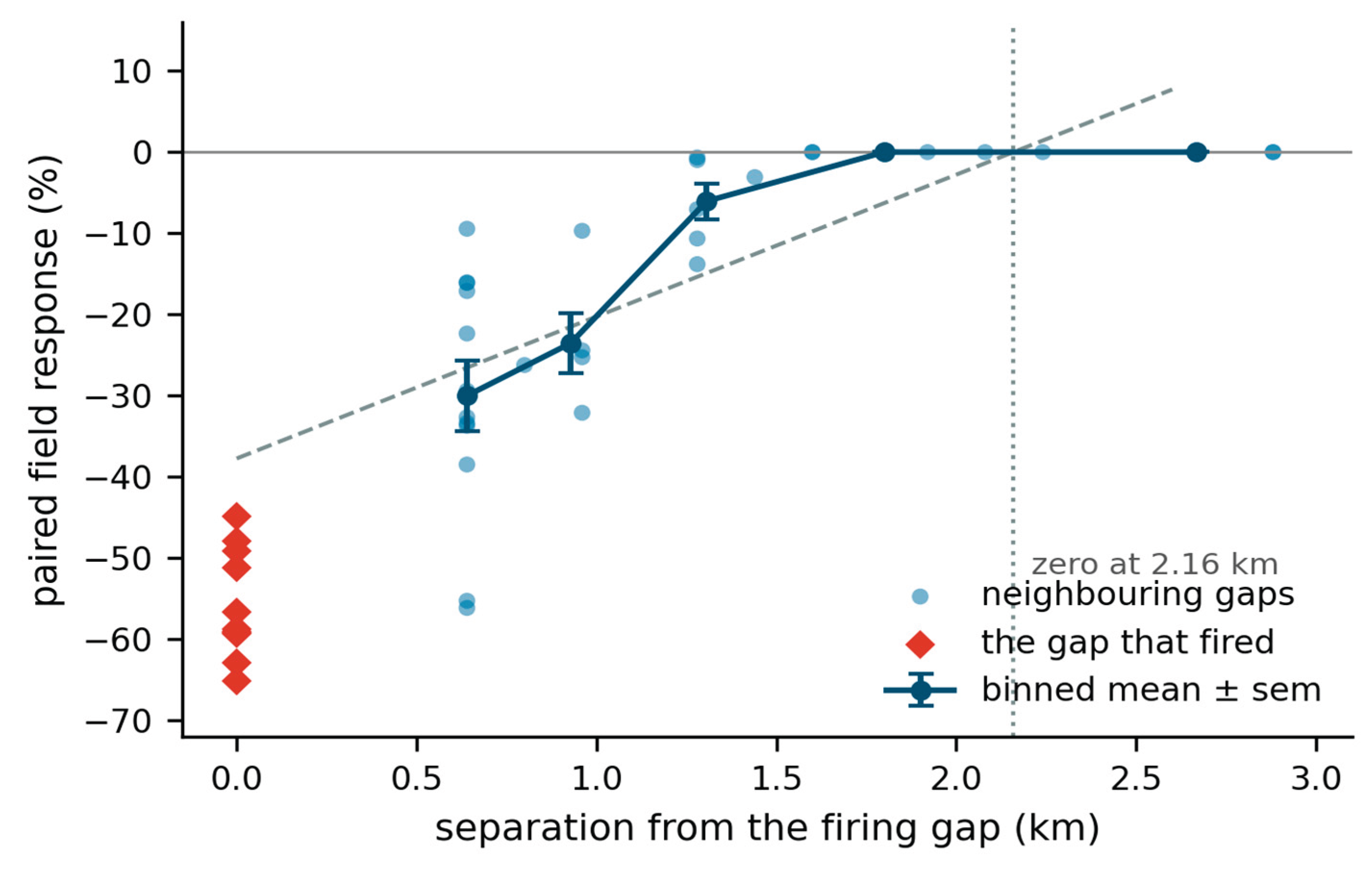
Whether this constitutes propagation was tested directly. With air filling the whole tube but ignition unrestricted, every gap in the column responded; with ignition confined to the firing gap, the neighbours gave +5, +0 and −4 per cent – nothing. Those two conditions look identical from the outside and are physically quite different, and only the confined-ignition figures in Table 5 are propagation.
6.3. Individual Trajectories
Every electron and ion was followed from birth: where it started, how far it travelled, how many layers it crossed and what ended it. Five seeds, 11,202 electrons and 5,601 ions.
Table 6.
Fate of individual electrons and ions, five seeds. Ranges are across seeds. The three electron fates separate by distance without anything having been imposed: those captured by a positive layer were born beside one and had nowhere to go.
Table 6.
Fate of individual electrons and ions, five seeds. Ranges are across seeds. The three electron fates separate by distance without anything having been imposed: those captured by a positive layer were born beside one and had nowhere to go.
| Fate | Share | Median life | Median path |
|---|---|---|---|
| Electrons – alive at the end | 53 – 57% | — | 1,243 – 1,431 m |
| Electrons – recombined with an ion | 35 – 36% | 55 – 61 steps | 464 – 510 m |
| Electrons – captured by a layer | 8 – 13% | 0 – 10 steps | 13 – 83 m |
| Ions – alive at the end | 67 – 71% | — | 5 – 8 m |
| Ions – neutralised by an electron | 29 – 33% | 84 – 93 steps | 4 – 10 m |
Electrons travel about 200 times further than ions – some 1,300 m against 7 m – over the same interval in the same field. That is the mass ratio of Sect. 2.4 doing what it should. The ions are effectively stationary space charge on the discharge timescale: they screen and wait to be neutralised, but carry the event nowhere. Everything that propagates is carried by electrons.
Figure 3.
Distance travelled by every carrier in one discharge. (a) Electrons against ions on the same axis: the medians differ by a factor of about two hundred, which is the electron-to-molecule mass ratio expressed as transport. (b) Electron paths separated by fate. Those captured by a positive layer travel almost nowhere because they were born beside one; those that recombine cover roughly half a gap; the survivors exceed a kilometre.
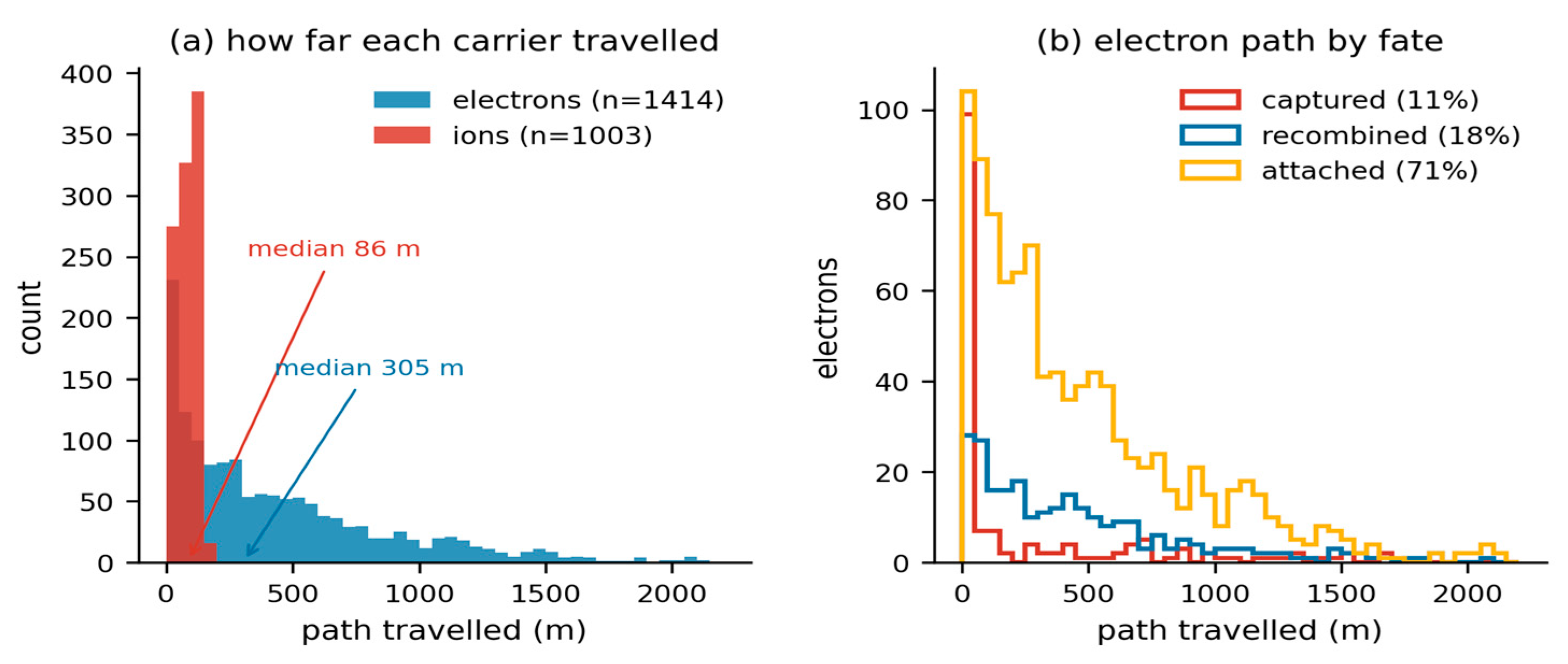
Between 32 and 40 per cent of electrons cross at least one charge layer, with a median path of 1,313 to 1,485 m among those that do and a maximum of 2,094 m. Ions cross in 1.7 to 2.5 per cent of cases and move 6 to 16 m when they do.
6.4. Why the Birthplace Decides Whether an Electron Can Travel
The potential along the tube was computed directly from the settled column. The swing across the column is 264 MV, which is the right order for a thundercloud and was not tuned to be. For an electron the potential energy is U = −eφ, so it sits highest in energy beside a negative layer and lowest mid-gap.
Table 7.
Energy an electron must have to reach the next site, computed from the axial potential of the settled column. The quantity is the climb relative to where the electron starts, not the peak-to-trough swing between gaps. Two of the five transitions from a negative layer cost nothing at all.
Table 7.
Energy an electron must have to reach the next site, computed from the axial potential of the settled column. The quantity is the climb relative to where the electron starts, not the peak-to-trough swing between gaps. Two of the five transitions from a negative layer cost nothing at all.
| Launched from | To | Energy required |
|---|---|---|
| Firing gap (φ maximum) | any neighbouring gap | 203 – 244 MeV |
| Negative layer, 6.63 km | 6.94 km | 0 MeV |
| Negative layer, 6.94 km | 7.86 km | 4.1 MeV |
| Negative layer, 7.86 km | 9.11 km | 41.0 MeV |
| Negative layer, 9.11 km | 10.50 km | 0 MeV |
The column therefore contains connected paths along which an electron travels at no energy cost. Which paths are available depends entirely on where the electron is born, and this is why some of the ionization must occur beside the layers: an electron born mid-gap is in a 200 MeV well and cannot leave, whatever the collisions do.
6.5. Cascade Structure
Each impact ionization is credited to the electron that caused it and flagged according to whether that electron had already crossed a layer; each new electron records its generation in the descent from a seed.
Between 24.8 and 27.6 per cent of all ionization occurs after the responsible electron has crossed a layer. That is new ionization in territory the seeds never occupied, produced by carriers that made the crossing, and it is the propagation step measured rather than inferred.
Table 8.
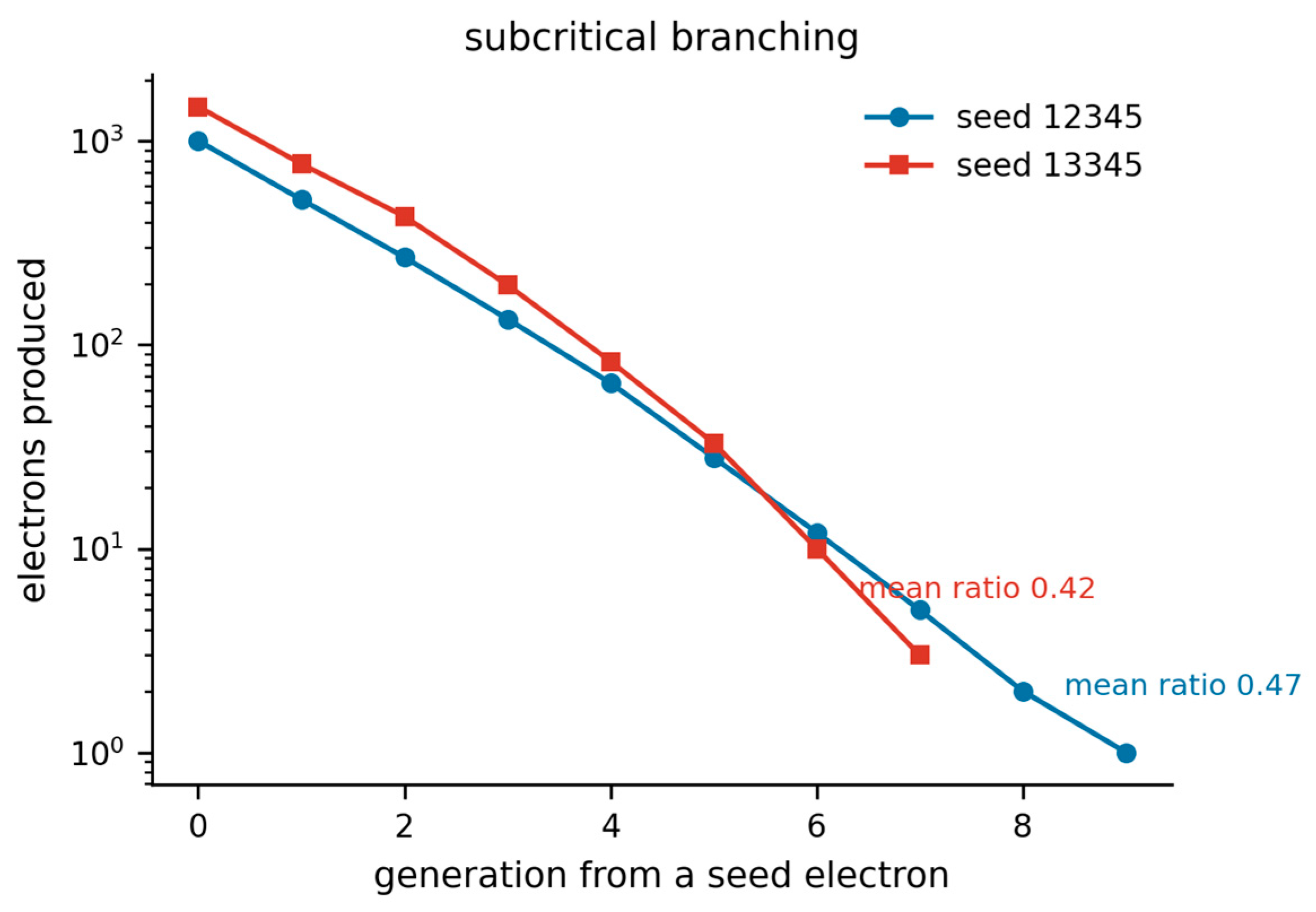
Cascade generations, where 0 is a seed electron from field ionization and each subsequent generation is produced by impact. Each generation is roughly half the previous one, sustained through seven to nine generations: subcritical branching, which is what produces events of finite and varied size rather than either fizzling or consuming the column.
| Seed | 0 | 1 | 2 | 3 | 4 | 5 | Deepest |
|---|---|---|---|---|---|---|---|
| 12345 | 1,003 | 517 | 269 | 134 | 65 | 28 | 9 |
| 13345 | 1,476 | 773 | 427 | 197 | 83 | 33 | 7 |
The branching ratio near 0.5 is worth dwelling on. A value just below unity is what a mechanism needs in order to produce events of finite, varied extent; the spatial expression of the same decay is the attenuation in Table 5. The decay is caused by electrons running out of energy and fuel, not by any cap.
Figure 4.
Electrons produced in each generation of the cascade, logarithmic ordinate. Generation zero is a seed electron from field ionization; each subsequent generation is produced by impact. The ratio between consecutive generations is close to one half and holds through seven to nine generations, which is subcritical branching sustained rather than either runaway or immediate extinction.
6.6. Termination Requires an Attachment Loss
Run to exhaustion rather than to a computational limit, the discharge does not stop. The electron population grows – 960 at the start, 1,492 after 400 ms – only 8 per cent of the fuel is consumed, and the front creeps at about 1,600 m s⁻¹. Two conclusions from an earlier, capped analysis must be corrected: the front speed measured over the first 80 ms is a transient of the opening phase, and the cascade is subcritical per generation but not in aggregate, because continued seeding replenishes the population faster than branching decays it. Without an electron loss term the model produces a sustained glow rather than an event.
Attachment on oxygen is the missing term, and it is the dominant electron loss in real air.
Table 9.
Effect of the attachment length. Without attachment the discharge never terminates. With it, duration and front speed become measurements rather than lower bounds, and both fall inside the interquartile range of the mapped storm in Table 11
at an attachment length of 30 model units.
Table 9.
Effect of the attachment length. Without attachment the discharge never terminates. With it, duration and front speed become measurements rather than lower bounds, and both fall inside the interquartile range of the mapped storm in Table 11
at an attachment length of 30 model units.
| Quantity | No attachment | Attach 1.2 km | Attach 2.4 km |
|---|---|---|---|
| Terminates | no | yes, 574 steps | yes, 1,348 steps |
| Duration | — | 229 ms | 539 ms |
| Front speed, advancing | 8.96 × 10³ m/s | 1.64 × 10⁴ m/s | 2.17 × 10⁴ m/s |
| Final reach | 1,285 m, rising | 845 m | 952 m |
| Firing gap | −59% | −52% | −58% |
| Neighbours | −7 / −16 / −10% | −2 / −5 / −8% | −2 / −7 / −9% |
Repeating the terminating configuration over ten seeds, every discharge ended by exhausting its electrons and none reached the safety limit. Table 10 gives the resulting statistics; they are measurements rather than bounds.
Figure 5.
Why the discharge needs an electron loss. (a) Free electrons against time. Without attachment the population grows and the event never ends; with attachment on oxygen it decays and the discharge terminates by exhaustion at 229 ms in this seed. (b) The ionization front. Both advance quickly for about 100 ms and then stall, which is what limits the reach; the unattached case continues to creep because electrons remain available.
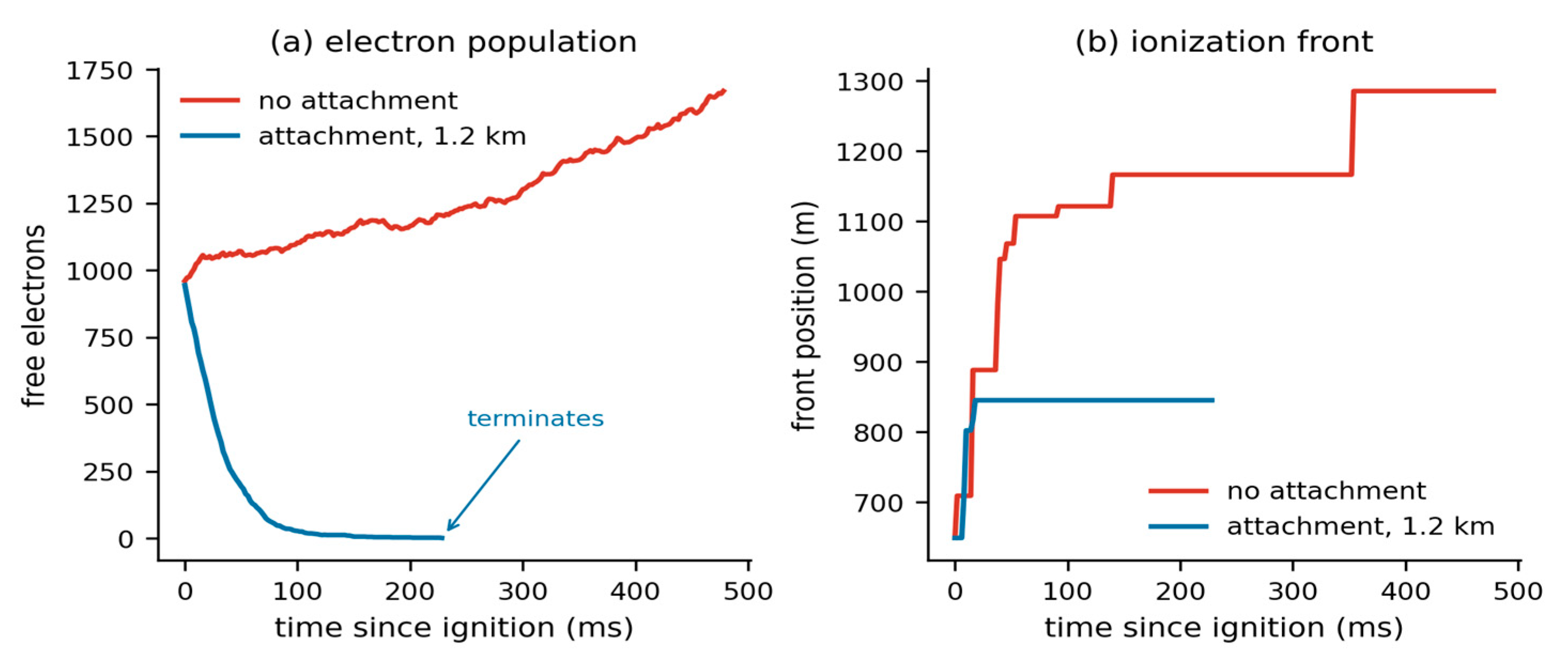
This introduces the central tension in the present state of the model: the term that makes the duration realistic is the term that suppresses the propagation. Without attachment the event spreads but never ends; with it the event ends on time and at the right speed but reaches a quarter as far as observation.
Note also that reach is not speed multiplied by duration – the median 1.44 × 10⁴ m s⁻¹ over the median 190 ms would be 2.7 km against 856 m measured. The front advances quickly for about 100 ms and then stalls while the population decays in place. Real flashes do show fast initial propagation followed by continued activity within the volume already reached, so the shape is not obviously wrong, but the stall is what costs the reach and it is not explained here.
6.7. Front Speed as a Prediction
Once the clock is fixed by the carrier drift velocity, the speed at which the leading edge of ionization advances is an output. A front cannot outrun its own carriers, so it must come in at or below 4 × 10⁴ m s⁻¹; where within that bound it falls is not something the model was told.
Over the advancing phase the model gives 3.8 × 10³ to 1.2 × 10⁴ m s⁻¹ without attachment, and a median 1.44 × 10⁴ m s⁻¹ over ten terminating discharges with it, against an observed range of 10⁴ to 10⁵ m s⁻¹ for in-cloud VHF source propagation. Section 7 makes the comparison against a specific dataset.
7. Comparison with Mapped Flashes
Two Lightning Mapping Array datasets are used: a West Texas winter storm of 24 December 2023 and an Oklahoma storm of 31 May 2017. Both are reduced with the model’s own definitions rather than compared against published flash statistics. This matters more than it may appear. Model quantities and published flash statistics are often defined differently – a per-iteration union of channel cells against a per-flash extent, or a layer thickness against a layer spacing – and comparing them directly manufactures agreement or disagreement that is an artefact of the definitions.
The model reports, for one discharge, an origin, a reach defined as the greatest displacement from that origin along the column axis, a duration from first to last ionization, and a front speed equal to reach divided by duration. The LMA is reduced identically: the first source of a flash is the origin, the reach is the greatest vertical displacement from it, and the duration is first to last source. Sources are retained at χ² ≤ 1 with at least six stations; flashes are clustered at Δt ≤ 0.15 s and Δr ≤ 3 km and kept if they contain at least ten sources. The instrument locates VHF sources in three dimensions by time of arrival across a network of stations (Rison et al., 1999); the quality cuts applied here follow the accuracy analysis of Thomas et al. (2004), which sets the location error against source altitude and station count.
Table 11.
Model against mapped flashes, both measured with the model’s definitions. Medians with interquartile ranges. The front speed is the quantity the model predicts once its clock is anchored; the reach is the quantity it gets wrong.
Table 11.
Model against mapped flashes, both measured with the model’s definitions. Medians with interquartile ranges. The front speed is the quantity the model predicts once its clock is anchored; the reach is the quantity it gets wrong.
| Quantity | Model | OKLMA 2017 | WTLMA 2023 |
|---|---|---|---|
| Flashes | 10 | 23 | 47 |
| Sources per flash | — | 12 (10–14) | 118 (23–493) |
| Front speed (m/s) | 1.44 × 10⁴ (1.2–1.8) | 2.05 × 10⁴ (1.6–2.7) | 1.69 × 10⁴ (1.1–2.4) |
| Duration (ms) | 190 (175–217) | 156 (131–188) | 192 (101–324) |
| Vertical reach (km) | 0.86 (0.78–0.89) | 3.21 (2.7–3.6) | 3.32 (2.6–4.3) |
| Initiation altitude (km) | 6.8 – 8.4 | 12.8 (11.1–14.8) | 5.36 (4.3–7.3) |
Front speed and duration both fall inside the WTLMA interquartile range. The duration medians are 190 ms against 192 ms, and the front speed medians differ by 15 per cent. Neither was fitted: the speed follows from a clock anchored on swarm data at a reduced field computed from the model’s own initiation altitude and threshold, and the duration follows from the attachment length required for the discharge to terminate at all.
The reach is short by a factor of about four. Since reach, speed and duration are not independent and two of the three agree, the discrepancy is localised rather than distributed: the front advances at very nearly the right speed for very nearly the right length of time, and then stops earlier in space than a real flash does. Three features of the model can produce that, and they are separable.
The first is the softened force law of Sect. 2.7. Softening at the carrier spacing removes the spurious near field, but it also removes the long coherent axial field that would accelerate an electron across several layer periods: the coherent component surviving softening is about three per cent of what a product feels locally, so the model systematically under-drives electrons that have already left the gap they were born in. The second is the absence of a conducting channel. A real bidirectional leader carries its own potential forward as it extends, so the field at the tip is regenerated rather than inherited, and the distance a flash travels is not bounded by the geometry of the gap that started it. The present model has no such object; its front can advance only as far as free electrons are carried by a field the discharge does not renew. The third is carrier density. Section 8.2 shows that below about 100,000 carriers the strongest fields sit at the layers rather than between them, so a front that has crossed one layer enters a region weaker than the sheet geometry assumes.
The first and third are testable within the present code. The second is not, and it is the reason this paper claims a mechanism for initiation and for local field relief rather than a mechanism for flash extent.
Initiation altitude overlaps the winter storm at its upper quartile and does not reach the Oklahoma storm at all. The model column tops out at 10.8 km, so a deep summer storm initiating near 13 km lies outside the configuration rather than contradicting it.
What the comparison does not establish should be stated alongside it. The observables are related but not identical. LMA sources are VHF emissions from fast breakdown and negative-leader processes; the model’s front is the leading edge of impact ionization, and a systematic offset between them would not be surprising. The clustering criteria are a common choice but not a published algorithm, and the results will shift somewhat with them. The Oklahoma dataset yields twelve sources per flash, which suggests a distant or poorly detected storm and argues for weighting it below the West Texas set. The model’s interquartile range for duration, 175 to 217 ms, is far narrower than the observed 101 to 324 ms: the model produces less variety than nature does, which is expected of a single configuration and is itself a limitation.
8. Sensitivity
8.1. Recombination Probability
Electron–ion recombination was initially certain whenever the two came within the collision radius. That is far too fast – two-body recombination in air has a coefficient of order 10⁻¹³ m³ s⁻¹, and free electrons are lost mostly to attachment rather than to positive ions – and it made recombination the dominant loss, holding ionizations and recombinations equal to within 0.1 per cent and killing every electron before it could travel.
Table 12.
Sensitivity to the recombination probability per encounter, same three seeds throughout. Across a factor of twenty the result moves by about one percentage point; it degrades only at unity, the unphysical extreme. The ionization count in the last column shows the recycling that certain-on-contact recombination produces.
| Probability | Firing gap | Neighbours < 1.1 km | Impact ionizations |
|---|---|---|---|
| 0.005 | −57.4% | −20.4% | 765 |
| 0.02 | −57.7% | −20.1% | 1,058 |
| 0.1 | −56.3% | −19.3% | 1,865 |
| 1.0 (certain) | −55.6% | −13.2% | 36,468 |
The spreading result therefore does not depend on the value chosen. It depends on recombination not being certain, which is a statement about physics rather than about a parameter.
8.2. Force Softening and Carrier Density
With point charges the field collapse is a single-iteration spike of about 26 per cent that has vanished by the next sample: a polarization transient. With softening at the carrier spacing it is smaller at the instant of the split and then persists and deepens, 5 to 13 per cent sustained over at least eight iterations. That is the difference between a dielectric response and a discharge, and it appears only once the spurious near field stops scattering the products.
Carrier density matters and is not innocent. Two oppositely charged sheets confine their field to the gap between them, which is the geometry the mechanism assumes, but a layer behaves like a sheet only when its carriers are packed closely relative to its distance from the opposing layer. The preference of the strongest fields for gap regions over layer regions rises from 0.50 at 20,000 carriers through 0.88 at 50,000 to 1.04 at 100,000. Below about 100,000 the field peaks at the layers rather than between them. The runs reported here use 30,000 carriers for tractability, which is below that crossing, and this is a real limitation rather than a detail: it means the trigger is not always located where the mechanism assumes.
That leaves the question of whether the softening length itself sets the result, which is the natural objection to Sect. 2.7: if the coherent axial field surviving softening is only three per cent of the local field, is the collapse an artefact of having suppressed the near field by a particular amount? Table 13 answers it directly. The paired experiment is repeated at three softening lengths spanning a factor of four, under a shortened protocol – a 400 sub-step cap and two host steps – chosen so that the three conditions cost the same and can be compared with each other. The shortened protocol gives a shallower collapse than the full runs of Sect. 6.1, so these figures should be read against one another rather than against the headline value.
Over a factor of four in softening length the collapse stays between −26 and −50 per cent, and such trend as there is runs towards a deeper collapse at longer softening. That is the opposite of what the objection predicts: if the collapse were an artefact of suppressing the near field, lengthening the softening would weaken it. The result is not an artefact of the value chosen. What the softening does change is the column, since it acts on the charging model as well as on the discharge, and the triggering gap is at a different altitude in each condition – so the invariance reported here is the stronger kind, across three different settled states rather than across one state treated three ways.
8.3. Air Fill Density
At an air fill equal to the hydrometeor density there are zero impact ionizations: electrons meet a hydrometeor and are captured before they find a molecule. The avalanche requires a fill well above unity, and this is physically correct, since real air molecules outnumber hydrometeors by some twenty orders of magnitude. The results here use a factor of ten.
9. Implications for Lightning Research
Three of the results above are statements about real storms rather than about the model, and each of the three can be tested against observations that have already been collected.
9.1. A structural Criterion for Initiation
Why lightning begins at fields near a tenth of the conventional breakdown value is the oldest unresolved question in the subject (Marshall et al., 1995; Petersen et al., 2008; Dubinova et al., 2015), and the explanations offered for it are local ones: field enhancement at the tips of elongated hydrometeors, runaway electrons seeded by cosmic ray showers, positive streamers launched from large ice particles. The result of Sect. 4 adds a condition of a different kind, geometric rather than microphysical, and independent of which of those local processes supplies the first electron. Identical charge, identical layers, identical spacing, identical carrier count: spread smoothly through each layer the structure produces 19 kV m⁻¹ and never fires, and gathered into local concentrations the same charge produces up to 196 kV m⁻¹ and does. What determines whether a gap can reach the ionization level is therefore not the layer-averaged field. It is the concentration of charge within the layer.
That is a claim about storms and it is falsifiable. It predicts that initiation should correlate with the small-scale heterogeneity of charge inside a layer rather than with the mean field across it, so that two soundings yielding the same layer-mean field should differ in initiation rate according to the structure within the layers. Balloon soundings resolve the electric field at metre scale and lightning mapping arrays locate initiation points to tens of metres. The two quantities can be placed side by side in data that already exists, without a new instrument or a new campaign.
9.2. What Stops a Flash
With the electron attachment loss removed the discharge does not terminate at all (Sect. 6.6): it exhausts the sub-step budget with its electron population still growing. With attachment on oxygen, every one of ten discharges terminates by exhausting its electrons, at a median 190 ms against 192 ms for the mapped winter storm. The attachment length was not fitted to the observed duration. It was bounded by the requirement that the discharge terminate at all, and the agreement in duration followed from that bound rather than being imposed on it.
If flash duration is set by dissociative attachment on oxygen rather than by channel geometry or by the quantity of charge available, then it should scale with the oxygen number density and so should fall with altitude. Flash duration and initiation altitude are both routine products of a lightning mapping array, which makes the predicted trend directly measurable in existing archives, and its absence would falsify the identification.
9.3. A Charge Budget That Closes
The stochastic dielectric-breakdown scheme used in cloud-resolving electrification models sets the charge inside the grown channel to zero, which removes net charge from the domain at every flash (Sect. 1). Any quantity that depends on the storm charge budget across more than one flash therefore inherits an unphysical sink: the recharge time between flashes, the equilibrium charge structure that the storm relaxes toward, and the flash rate that follows from both. Flash rate is precisely the statistic that lightning parameterizations in weather and climate models are asked to deliver.
The scheme described here conserves charge at every reaction by construction, and conservation is asserted in code at each event rather than assumed to hold. It is not offered as a drop-in replacement for a breakdown lattice – it is far more expensive, and Sect. 10 sets out what it does not yet do – but it establishes that a charge-conserving discharge is achievable inside a particle model, and it provides a reference against which the charge error of a cheaper scheme can be measured rather than tolerated.
None of the three depends on the reach agreeing with observation. The shortfall reported in Sect. 7 bounds what this model can say about how far a flash travels. It does not bear on where flashes begin, on what brings them to an end, or on whether charge is conserved while they proceed.
10. Limitations
The charging model is a layer generator, and the discharge results are conditional on the layered structure it produces rather than on the process that produced it. That conditionality is demonstrated and not merely asserted: Sect. 4 runs the identical discharge on layers assembled by hand in a column no vortex has ever acted on, and the discharge behaves the same way. The structure it requires is also observed independently of any model, since balloon soundings find four to six alternating layers of a few hundred metres in real storms (Stolzenburg et al., 1998). The mechanism therefore rests on a measured feature of thunderclouds rather than on a modelled one.
Gravity is nonetheless zero in the runs reported here, and its absence should be placed correctly rather than either dismissed or overstated. Differential sedimentation of oppositely charged graupel and ice crystals is what atmospheric electricity credits with building the storm-scale vertical dipole (Takahashi, 1978; Saunders et al., 2006), and a model without it cannot claim to reproduce that structure, nor the cloud-to-ground discharge that spans it. It is a weaker constraint on what is examined here. The mechanism acts on the field in the gap between two adjacent layers a few hundred metres apart, and the events it is compared against in Sect. 7 are intracloud flashes propagating within and between such layers. For that geometry the quantities that matter are the layer spacing and the concentration of charge inside the layers, both specified in Sect. 4 and matched to observation, and not the buoyancy-driven process that set the layer altitudes in the first place. The absence of gravity bounds what the charging model may claim about the large-scale charge structure. It does not bound the discharge result, which begins after that structure exists.
The carriers themselves remain coarse. They have no size spectrum and no fall speeds, their charge-to-mass ratio is far from that of real hydrometeors, and each stands for of order 10¹⁰ of them, so a contact between two carriers is not a hydrometeor collision. This is why the charging component is described as a generator of layered structure and not as a microphysical model of electrification.
Within the discharge itself, four limitations are worth naming. The model produces no light, so it cannot be compared against optical or VHF observations except through the geometric proxies used in Sect. 6. It produces one event per run and cannot generate a flash rate, which is the statistic most often reported for real storms. All propagation measured is axial, whereas intracloud flashes propagate horizontally through charge layers at least as much as vertically. And the model contains no conducting channel: a real leader carries its own potential forward as it extends, which is how charge crosses the hundred-megavolt structures measured in Sect. 6.4, and nothing here corresponds to that object.
The drift velocity on which the clock is anchored is the single external constant in the model. It is not measured here and it is not derived here; it is taken to be 4 × 10⁴ m s⁻¹ at 27 Td on the strength of dry-air swarm compilations, and every duration reported scales inversely with it while every speed scales with it. A two-term Boltzmann solution for the exact mixture, temperature and reduced field would fix it to better than the ten per cent that separates published cross-section sets, and until that is done the absolute durations quoted here should be read as accurate to a factor of order unity. Nothing else in the paper depends on it: the field collapse, the attenuation length, the path-length ratio, the crossing fractions and the generation depth are all dimensionless or in metres, and are unaffected.
11. Conclusions
A discharge scheme built from ionization of the air between charge layers, with no channel and no propagation rule, conserves charge exactly and produces localised events that relieve the field where they start and, to a lesser degree, for about two kilometres on either side. What it requires of the charge structure is layering together with local concentration within the layers: a hand-built smooth layered column carrying identical charge produces a field an order of magnitude too small and never discharges, while gathering the same carriers into concentrations raises the field tenfold. Two quantities that would ordinarily be free are derived: the separation at which a newly created pair is unbound, from the balance between its own Coulomb field and the ambient; and the timestep, from the electron drift velocity at the reduced field the model itself produces.
Individual trajectories show the transport asymmetry that the electron-to-molecule mass ratio requires, with electrons travelling some two hundred times further than ions, a third of them crossing a charge layer, and a quarter of all ionization occurring beyond the layer the responsible electron was born behind. The cascade is subcritical per generation at a branching ratio near one half, sustained through seven to nine generations.
Without an electron attachment loss the discharge does not terminate. With attachment on oxygen every one of ten discharges terminates by exhausting its electrons, at a median duration of 190 ms and a median front speed of 1.44 × 10⁴ m s⁻¹ against 192 ms and 1.69 × 10⁴ m s⁻¹ for flashes measured in a mapped winter storm using the model’s own definitions, and neither quantity was fitted to it. The reach remains a factor of four short, and the term that makes the duration realistic is the term that suppresses the propagation. That tension, and the stall that produces it, are the clearest open problems this work leaves.
Author Contributions
NH designed the study and the discharge mechanism, wrote the model and the analysis code, performed all simulations, carried out the analysis, and prepared the manuscript.
Financial support
This research received no specific grant from any funding agency in the public, commercial, or not-for-profit sectors.
Code and data availability
The Thunder model v1.0, the analysis scripts, the Lightning Mapping Array reduction described in Sect. 7 and the configuration for every run reported here are archived at Zenodo (Harkiolakis, 2026). The model is written in Python 3 and depends only on NumPy; it runs on a single core of a standard desktop computer, and the longest run reported here completes in under ten minutes. Licence: [to be stated at deposit]. A browser implementation of the same scheme, in which the twelve parameters listed in Sect. 2 are fixed in source and not exposed through the interface, is included in the archive as a single self-contained HTML file so that the results can be replicated without installing anything. Every result in this paper regenerates from the deposited code with the commands listed in the archive README. The random number generator is seeded deterministically, so a given seed reproduces a bit-identical column and a bit-identical discharge. The Lightning Mapping Array observations used in Sect. 7 are from the West Texas LMA for 24 December 2023 and the Oklahoma LMA for 31 May 2017; the reduced source files and the clustering script that produced Table 11 from them are included in the same archive.
Acknowledgments
Large language model assistance (Anthropic Claude) was used in implementing and debugging the simulation code, in executing and tabulating the numerical experiments reported here, and in editing the text. The author specified the mechanism, designed and directed every experiment, verified the results, and takes full responsibility for the content of this paper.
Competing interests
The author declares that they have no conflict of interest.
References
- Dubinova, A., Rutjes, C., Ebert, U., Buitink, S., Scholten, O., and Trinh, G. T. N.: Prediction of lightning inception by large ice particles and extensive air showers, Phys. Rev. Lett., 115, 015002, 2015. [CrossRef]
- Dutton, J.: A survey of electron swarm data, J. Phys. Chem. Ref. Data, 4, 577–856, 1975. [CrossRef]
- Hagelaar, G. J. M. and Pitchford, L. C.: Solving the Boltzmann equation to obtain electron transport coefficients and rate coefficients for fluid models, Plasma Sources Sci. Technol., 14, 722–733, 2005. [CrossRef]
- Harkiolakis, N.: Thunder v1.0: a particle model of thundercloud charging with a charge-conserving gap-ionization discharge, Zenodo [code], 2026. [CrossRef]
- Iudin, D. I., Rakov, V. A., Syssoev, A. A., Bulatov, A. A., and Hayakawa, M.: Formation of decimeter-scale, long-lived elevated ionic conductivity regions in thunderclouds, npj Clim. Atmos. Sci., 2, 46, 2019. [CrossRef]
- Kasemir, H. W.: A contribution to the electrostatic theory of a lightning discharge, J. Geophys. Res., 65, 1873–1878, 1960. [CrossRef]
- MacGorman, D. R. and Rust, W. D.: The Electrical Nature of Storms, Oxford University Press, New York, 432 pp., ISBN 9780195073379, 1998.
- Mansell, E. R., MacGorman, D. R., Ziegler, C. L., and Straka, J. M.: Simulated three-dimensional branched lightning in a numerical thunderstorm model, J. Geophys. Res., 107, 4075, 2002. [CrossRef]
- Marshall, T. C., McCarthy, M. P., and Rust, W. D.: Electric field magnitudes and lightning initiation in thunderstorms, J. Geophys. Res., 100, 7097–7103, 1995. [CrossRef]
- Niemeyer, L., Pietronero, L., and Wiesmann, H. J.: Fractal dimension of dielectric breakdown, Phys. Rev. Lett., 52, 1033–1036, 1984. [CrossRef]
- Petersen, D., Bailey, M., Beasley, W. H., and Hallett, J.: A brief review of the problem of lightning initiation and a hypothesis of initial lightning leader formation, J. Geophys. Res., 113, D17205, 2008. [CrossRef]
- Pitchford, L. C., Alves, L. L., Bartschat, K., Biagi, S. F., Bordage, M.-C., Bray, I., Brion, C. E., Brunger, M. J., Campbell, L., Chachereau, A., Chaudhury, B., Christophorou, L. G., Carbone, E., Dyatko, N. A., Franck, C. M., Fursa, D. V., Gangwar, R. K., Guerra, V., Haefliger, P., Hagelaar, G. J. M., Hoesl, A., Itikawa, Y., Kochetov, I. V., McEachran, R. P., Morgan, W. L., Napartovich, A. P., Puech, V., Rabie, M., Sharma, L., Srivastava, R., Stauffer, A. D., Tennyson, J., de Urquijo, J., van Dijk, J., Viehland, L. A., Zammit, M. C., Zatsarinny, O., and Pancheshnyi, S.: LXCat: an open-access, web-based platform for data needed for modeling low temperature plasmas, Plasma Process. Polym., 14, 1600098, 2017. [CrossRef]
- Rison, W., Thomas, R. J., Krehbiel, P. R., Hamlin, T., and Harlin, J.: A GPS-based three-dimensional lightning mapping system: initial observations in central New Mexico, Geophys. Res. Lett., 26, 3573–3576, 1999. [CrossRef]
- Saunders, C. P. R., Bax-Norman, H., Emersic, C., Avila, E. E., and Castellano, N. E.: Laboratory studies of the effect of cloud conditions on graupel/crystal charge transfer in thunderstorm electrification, Q. J. Roy. Meteor. Soc., 132, 2653–2673, 2006. [CrossRef]
- Stolzenburg, M., Rust, W. D., and Marshall, T. C.: Electrical structure in thunderstorm convective regions: 3. Synthesis, J. Geophys. Res., 103, 14097–14108, 1998. [CrossRef]
- Takahashi, T.: Riming electrification as a charge generation mechanism in thunderstorms, J. Atmos. Sci., 35, 1536–1548, 1978. [CrossRef]
- Thomas, R. J., Krehbiel, P. R., Rison, W., Hunyady, S. J., Winn, W. P., Hamlin, T., and Harlin, J.: Accuracy of the Lightning Mapping Array, J. Geophys. Res., 109, D14207, 2004. [CrossRef]
- Williams, E. R.: The tripole structure of thunderstorms, J. Geophys. Res., 94, 13151–13167, 1989. [CrossRef]
Figure 1.
The input state, 30,000 carriers after 110 iterations. (a) Charged carriers in a radial-axial section. The charge occupies an annulus between about 2 and 4 km radius and is gathered into dense filaments rather than spread smoothly. (b) Net charge per axial band, with the gaps between consecutive layers of opposite sign shaded; those gaps are what the discharge scheme acts on.
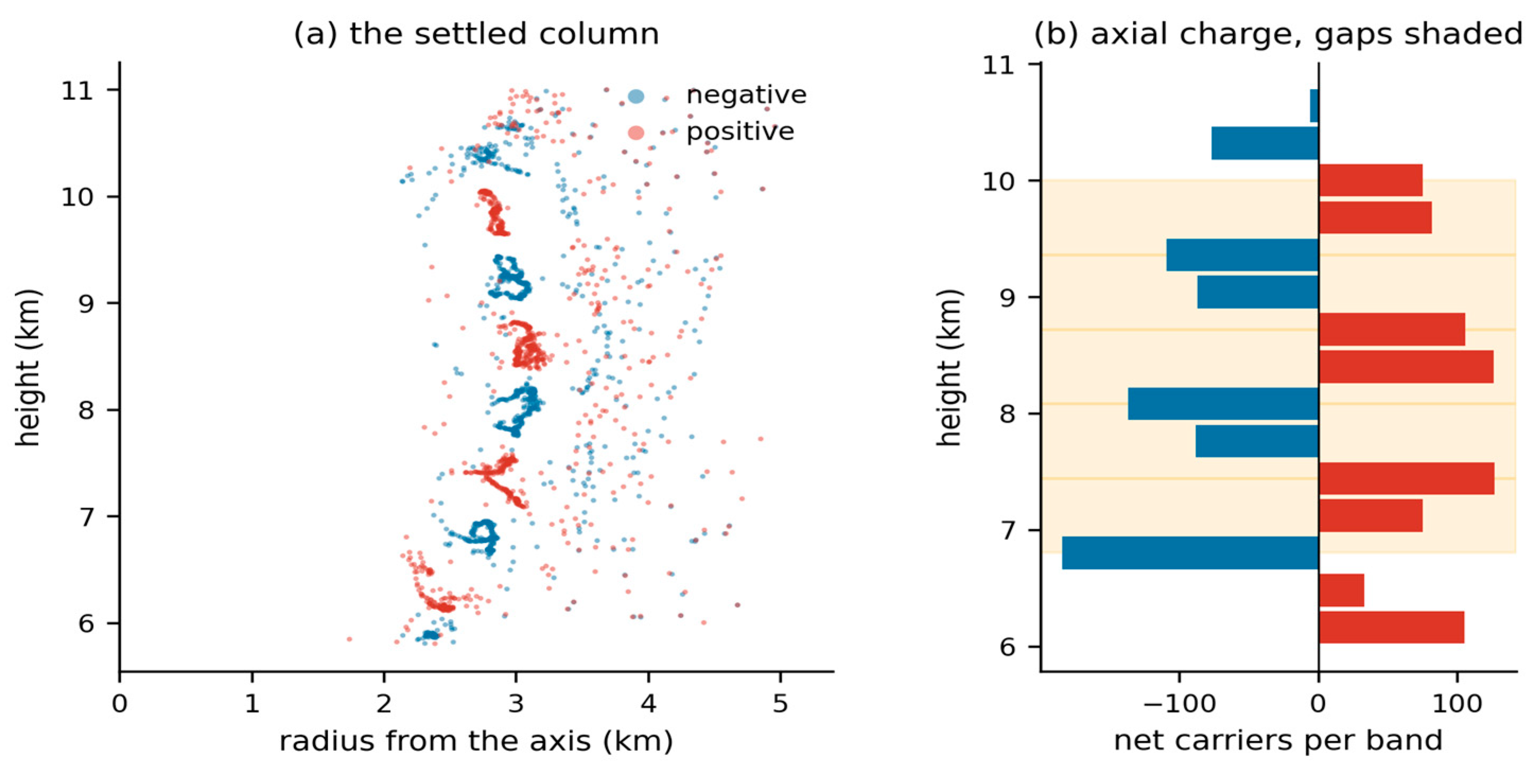
Table 1.
The charging model in full. Lengths are in model units of 40 m and the timestep is the product of dt and the speed multiplier. Nothing else is required to reproduce the column.
Table 1.
The charging model in full. Lengths are in model units of 40 m and the timestep is the product of dt and the speed multiplier. Nothing else is required to reproduce the column.
| Quantity | Value | Note |
|---|---|---|
| Carriers | 30,000 | sensitivity in Sect. 8.2 |
| Domain | 400 × 400 × 260 u | 16 × 16 × 10.4 km |
| Metres per unit | 40 | length anchor |
| Timestep | dt 0.05 × speed 20 | one host iteration ≈ 24 s |
| Column base, top | 150, 270 u | 6.0, 10.8 km |
| Core radius, base to top | 5 to 25 u | concavity exponent 0.7 |
| Circulation | spin 2.4 | Rankine, constant circulation |
| Updraft | 4 u/s | Gaussian about the core wall |
| Radial inflow strength | 55 | pressure-driven term |
| Gravity | 0 | see Sect. 8 |
| Coulomb constant | 12 | model units |
| Biot–Savart constant | 0.35 | small correction at these speeds |
| Interaction cutoff | 15 u | 600 m |
| Force softening | 6 u | 240 m, Sect. 2.7 |
| Contact radius | 2 u | 80 m |
| Refractory period | 60 steps | after a charge exchange |
| Charge anchor | 1 nC m⁻³ | gives 0.349 C per carrier |
Table 5.
Field response against distance from the firing gap, pooled over eleven seeds. Ignition was confined to the firing gap and its two bounding layers, so a response elsewhere is propagation rather than independent ignition. The firing gap itself falls 55.8 per cent, standard deviation 6.5.
Table 5.
Field response against distance from the firing gap, pooled over eleven seeds. Ignition was confined to the firing gap and its two bounding layers, so a response elsewhere is propagation rather than independent ignition. The firing gap itself falls 55.8 per cent, standard deviation 6.5.
| Separation | n | Mean response | sem | t |
|---|---|---|---|---|
| 0.6 – 0.7 km | 12 | −30.0% | 4.3 | −6.95 |
| 0.7 – 1.1 km | 5 | −23.5% | 3.7 | −6.34 |
| 1.1 – 1.6 km | 6 | −6.0% | 2.2 | −2.74 |
| 1.6 – 2.2 km | 4 | 0.0% | — | — |
| beyond 2.2 km | 3 | 0.0% | — | — |
Table 10.
Ten terminating discharges. Every one ended by exhausting its electrons; none reached the safety limit, so duration and reach are measurements rather than lower bounds. Attachment length 1.2 km, 30,000 carriers.
Table 10.
Ten terminating discharges. Every one ended by exhausting its electrons; none reached the safety limit, so duration and reach are measurements rather than lower bounds. Attachment length 1.2 km, 30,000 carriers.
| Quantity | Median | IQR | sd |
|---|---|---|---|
| Trigger field (kV m⁻¹) | 331 | 278 – 384 | 58 |
| Duration (ms) | 190 | 175 – 217 | 26 |
| Front speed, advancing (m/s) | 1.44 × 10⁴ | 1.18 – 1.75 × 10⁴ | 8.0 × 10³ |
| Final reach (m) | 856 | 780 – 886 | 83 |
| Hydrometeors neutralised | 167 | 135 – 180 | 31 |
| Impact ionizations | 402 | 302 – 438 | 117 |
| Charge transferred (C) | 58 | — | 39 – 71 range |
| Charge moment (C km) | 48 | — | 29 – 59 range |
Table 13.
Collapse of the field in the firing gap at three softening lengths, identical shortened protocol and identical seeds throughout. The softening also alters the settled column, so these are three columns rather than one column under three force laws; the discharge is measured on whatever column each condition produces.
| Seed | ε = 3 u (120 m) | ε = 6 u (240 m) | ε = 12 u (480 m) |
|---|---|---|---|
| 12345 | −37% | −30% | −50% |
| 13345 | −26% | −36% | −48% |
| mean | −31% | −33% | −49% |
Disclaimer/Publisher’s Note: The statements, opinions and data contained in all publications are solely those of the individual author(s) and contributor(s) and not of MDPI and/or the editor(s). MDPI and/or the editor(s) disclaim responsibility for any injury to people or property resulting from any ideas, methods, instructions or products referred to in the content. |
© 2026 by the author. Licensee MDPI, Basel, Switzerland. This article is an open access article distributed under the terms and conditions of the Creative Commons Attribution (CC BY) license.
Copyright: This open access article is published under a Creative Commons CC BY 4.0 license, which permit the free download, distribution, and reuse, provided that the author and preprint are cited in any reuse.