

Submitted:
10 September 2026
Posted:
14 September 2026
You are already at the latest version
Abstract
This paper investigates a nonlinear strong prescribed-time cooperative control theory, aiming to achieve spatio-temporal consistency in multi-agent control under disturbance. Taking multiple unmanned surface vessels(USVs) as the application object, a strong prescribed-time cooperative target-guided coordinate control(SPT-TACC) method is proposed to ensure that USVs can complete the cooperative target tracking task at the prescribed time. First, the error models of the cooperative kinematic subsystem and the kinetic subsystem are converted into periodic delayed forms, and a strong prescribed-time cooperative control system based on periodic delayed feedback is designed, enabling each USV to arrive at the desired tracking point simultaneously at the prescribed time. Second, a complete stability proof is provided for the nonlinear strong prescribed-time cooperative control theory with physical constraints. Finally, an empirical formula for the lower bound of the prescribed convergence time of the system with physical constraints is summarized, and the rules for setting the prescribed convergence time of each subsystem are summarized to avoid the divergence problem of the control system caused by unreasonable settings of multiple prescribed time. Simulation comparison results effectively verify the effectiveness of the proposed control method.
Keywords:
strong prescribed-time stability
; target-guided coordinate control
; unmanned surface vehicles
; distributed control
1. Introduction
With the continuous advancement of technologies such as sensors, network communication, automatic control, and artificial intelligence, unmanned systems technology has developed rapidly in recent years. However, facing increasingly complex and diverse task requirements, the limitations of individual intelligent agents are gradually becoming apparent: 1) limited endurance, small operating area, and low execution efficiency; 2) limited individual space, unable to carry the payload required for large tasks; 3) limited individual performance redundancy, unable to maintain operational continuity in the event of individual failures, and poor fault tolerance[1]. Therefore, the collaborative capabilities of multiple intelligent agents urgently need to be improved to adapt to the demands of future complex tasks[2].
As a typical type of unmanned maritime equipment, unmanned surface vessels are a key node in the future connection of unmanned swarm systems in the air, on the water, on land, and underwater. Multiple USVs can perform military and civilian tasks such as collaborative anti-submarine warfare, target encirclement, fleet escort, target guard, collaborative resource exploration, and collaborative search and rescue[3,4]. However, Multiple USVs cooperative control technology is still in the theoretical and model experiment stage, and there is still a gap before it can be applied on a large scale. Factors such as nonlinear disturbance[5], constraints on the physical characteristics of USVs[6], and spatio-temporal consistency of cooperative operations[7] will affect the success rate of mission execution, leading to serious consequences such as non-cooperative targets escaping, escort targets being interfered with, and search and rescue targets being lost.
Taking multi-USV target-guided coordinate control(TACC) as an example, the initial research on the convergence of the control system mainly focused on the speed of convergence, that is, how to enable each USV to reach the desired tracking point as soon as possible and achieve spatial consistency. Zhu et al.[8] proposed a finite-time TACC system, which enables each USV to form the desired tracking formation faster than the traditional asymptotic convergence control system. Gao et al. designed a fixed-time cooperative control system based on an edge-triggered extended state observer, which enables multiple USVs to quickly recover their original formation after communication is attacked[9]. Existing control methods based on asymptotic stability and finite/fixed-time stability theory cannot guarantee that the system error will converge at a time set by the user, i.e., they cannot achieve time consistency. To address this problem, Zhao et al. designed a prescribed-time extended state observer, which enables each USV to complete the estimation of time-varying disturbance before the prescribed time[10]. Yang et al. designed a distributed prescribed-time observer in the cooperative kinematic control subsystem to quickly estimate uncertain dynamics and target states, and a reduced-order prescribed-time estimator in the kinematic control subsystem to quickly estimate unmodeled dynamics[11]. Unlike the literature[10,11], Xing et al. designed a prescribed-time pursuit and escape control law, which enables the non-cooperative target to be intercepted before the prescribed time[12]. Li et al. designed a prescribed time cooperative encirclement control law, which enables each USV to surround the target before the prescribed time[13]. Nie et al. and Sui et al. designed time-varying prescribed performance functions and proposed an improved prescribed-time extended state observer to accurately estimate the unmeasurable velocity of the target and external disturbance, and improve the convergence speed of the control system[14,15]. Existing research based on prescribed time stability theory can only guarantee that each USV arrives at the mission area before the prescribed time, but it cannot achieve consistent convergence time.
Based on the prescribed-time control method, Ding et al. take the nonlinear single-input single-output control system as the research object, introduce the past state of the system into the model, formed a periodic delayed control system, and proposed a strong prescribed-time control method, which enables the system errors to converge accurately at a time set by human in an undisturbed environment[16]. Zhao et al. and Ding et al. design a strong prescribed-time controller for linear time-delay systems, achieving convergence of system errors at a prescribed time[17,18]. Dong et al., focusing on multi-input multi-output linear systems, design a fault-tolerant strong prescribed-time controller capable of achieving system errors convergence at a prescribed time even under actuator failure[19]. At the kinematic control layer, Zheng et al. design a strong prescribed-time guiding law, achieving precise convergence of desired angles and angular velocities at a manually set time[20]. At the dynamic control layer, Peng et al. designed a linear reduced-order strong prescribed-time observer, effectively achieving accurate estimation of disturbance at a prescribed time[21]. Zhang et al. further designed a nonlinear strong prescribed-time observer to accurately compensate for disturbance caused by model uncertainties and actuator failures[22].
Motivated by the above mentioned works, this paper aims to propose a SPT-TACC method for USVs, which consists of several key components: (i) a strong prescribed-time cooperative control system based on periodic delayed feedback is designed, enabling each USV to arrive at the desired tracking point simultaneously at the prescribed time. (ii) simultaneously considering nonlinear disturbance and individual physical constraint characteristics, the overall stability of SPT-TACC is analyzed based on Lyapunov theory, providing theoretical support for the nonlinear strong prescribed-time cooperative control method. (iii) empirical formulas and setting rules are provided for prescribed time parameters for multi-level collaborative control systems, effectively avoiding system divergence problems caused by unreasonable prescribed time parameters and enhancing the robustness of collaborative control systems.
Compared to the existing research, the salient features of the proposed method are as follows: (i) different from [8,9,10,11,12,13,14,15], this paper introduces strong prescribed-time theory into a multi-USV TACC system for the first time, effectively achieving spatio-temporal consistency by ensuring that each USV reaches the desired tracking point at the prescribed time. (ii) Compared to [16,17,18,19,20,21,22], this paper focuses on a nonlinear cooperative control system with physical constraints and underactuated characteristics and provides a complete stability analysis, verifying that the errors of this type of control system can converge at the prescribed time. (iii) Based on [16,17,18,19], this paper further presents empirical formulas and rules for setting the prescribed time parameters of each subsystem in a multi-level cooperative control system, providing theoretical support for the safe and stable application of this method in future practical engineering.
2. Preliminaries And Problem Formulation
2.1. Graph Theory
The communication topology diagram includes nodes and edges. Each USV can be considered as a node, and the communication links between USVs can be considered as edges. There are USVs labeled to , with as the node set and as the edge set. To facilitate the representation of whether a communication link exists between USVs, an adjacency matrix is defined. If , , otherwise, . To represent the links between USVs and the target, A matrix is defined. If the USV can directly detect the target's location, , otherwise, .
2.2. Kinematic and Kinetic Models for USVs
Assume that all USVs are isomorphic. Define as a position vector, where is the surge position, is the sway position, and is the heading angle. Define as a velocity vector, where is the surge velocity, is the sway velocity, and is the yaw velocity. The kinematic model of the USV can be described as:
The sideslip angle is defined as . Considering the effect of the drift angle, Equation 1 can be rewritten as:
where is the total velocity.
The kinetic model is given by:
where , , are the additional mass. , , are hydrodynamic damping. is the control force, including the surge force and the yaw moment . is the time-varying disturbance matrix.
2.3. Problem Formulation
The schematic diagram of the SPT-TACC system is shown in Figure 1. is the north-east-down coordinate and is the body-fixed coordinate. Define the position vector of the USV in the northeast coordinate system as . Define the position vector of the target as . Define the target's heading as 。Once one of USVs locates the target, each USV must proceed to its corresponding desired tracking point in the vicinity of the target. Define the desired tracking point position vector as , which is uniformly distributed on a circle with radius centered on the target. The desired tracking points adjust their orientation based on the target's real-time heading; that is, the formation is time-varying in the north-east-down coordinate system but can be regarded as a stable formation in the body-fixed coordinate system.
Taking the moment when the target is detected by USVs as the initial time, the position vector of the target at the initial time can be expressed as , and its initial heading as . The initial position vector of the desired tracking point can be expressed as:
where is the desired angle between the distance vector from the USV to the target and the target's heading.
Based on Equation 4, the position vector of the desired tracking point at subsequent time instants can be expressed as:
To implement SPT-TACC, the following four control objectives must be met.
(1)Prescribed-time location consistency target: Ensure that the USV arrives at the desired tracking point at the prescribed time , and maintains the TACC formation with the other USVs after :
where is the desired distance between USVs. is the desired distance among USVs and the target. is the tracking point position corresponding to the USV.
(2)Prescribed-time velocity consistency target: Ensure that the USV can keep up with the target's velocity at the prescribed time and maintain the same velocity after :
2.4. Definitions and Lemmas
Lemma 1.[16] Considering the following nonlinear delayed system:
where is the control input, is the state vector, is the initial condition.
Suppose that there is a positive definite function such that:
where , and are some constants, , is a self-defined periodic function and . Then, the system Equation 8 with is fixed-time stable with the settling time .
Lemma 2. Considering the following uncertain scalar nonlinear system:
Let be the prescribed time. The control law is designed as follows:
where , , and is estimated value of . If holds, the system consisting of Equation 10 and Equation 11 is strong fixed-time stable with the settling time .
Proof of Lemma 2. Choose the Lyapunov function . Then, it is obtained from Equation 10 and Equation 11 that:
If , then it is obtained from Equation 12 that:
According to Lemma 1, the system consisting of Equation 3 and Equation 4 is strong fixed-time stable with the settling time . □
Remark 1. When is independent of the system state , the prescribed convergence time of the disturbance estimate only needs to satisfy . In particular, when the disturbance estimate is related to the system state , the prescribed convergence time of the disturbance estimate must be consistent with the prescribed convergence time of the system.
Remark 2. Multi-USV cooperative control systems are typical strongly nonlinear control systems with state constraints. The convergence time of system errors has an explicit functional relationship with the system's initial state and state constraints. Taking the maximum resultant velocity constraint of the USV as an example, the USV needs time to travel to the desired tracking point at its maximum resultant velocity. If the prescribed convergence time is , the system will fail to meet the convergence condition, leading to system divergence. Therefore, the multi-USV strong prescribed-time cooperative control system needs to set a lower bound for the convergence time , and the prescribed convergence time of each error subsystem should not be less than .
Based on the maneuverability constraints of each USV, the empirical formula for the lower bound of the prescribed convergence time can be summarized as follows:
where is the prescribed convergence time for the error subsystem.
3. Strong Prescribed-Time Collaborative Controller Design
3.1. Strong Prescribed-time Kinematic Control Law Design
Based on graph theory, considering the position tracking errors and the velocity tracking errors among USVs and target, the collaborative kinematic control error is given as follows:
where is the position tracking error. is the velocity tracking error. is the coordinate rotation matrix.
The differentiation of Equation 15 follows that:
where is an identity matrix.
Note that Equation 16 does not include the heading information of USVs, and the distributed kinematic control law applicable to underactuated USVs cannot be derived solely from Equation 16. Therefore, an auxiliary variable is introduced into the collaborative kinematic error:
Substituting the differentiation of Equation 17 into Equation 16, it follows that:
where . . . is a small positive parameter.
To quickly and accurately estimate the time-varying sideslip angle in Equation 18, a prescribed-time extended state observer(PTESO) is introduced as follows:
where is the estimation error of heading angle. is the estimation error of sideslip angle. and are positive parameters. and are the estimated values of the heading angle and the sideslip angle, respectively. and are the predefined time. is a prescribed-time adjustment function, which is designed as follows:
Remark 3. All errors in Equation 19 converge before the prescribed time . The prescribed-time ESO of the above design and its stability proof can be found in our previous work[23].
Note that Equation 18 includes acceleration information for both USVs and the target. To avoid chattering in the distributed kinematic control output due to acceleration information, a first-order low-pass filter is introduced as follows:
where is the time constant. is the filtered speed value of USVs and the target.
Substituting Equations 19 and Equations 21 into Equation 18, the collaborative kinematic error model can be rewritten as follows:
According to Lemma 2, Equation 22 can be rewritten as follows:
Based on Equation 23, a nonlinear periodic delayed cooperative kinematic error is given as:
where is the value of periods of kinematic subsystem delayed. When , . is the Initial system state value.
Define the collaborative kinematic error as . Based on Equation 24, the following strong prescribed-time cooperative kinematic control law based on periodic delayed feedback can be designed as:
where is the desired velocity vector. is a positive parameter. is the estimated value of the time-varying disturbance. , and are defined as follows:
where , , and are positive parameters. is a 2-periodic function. and can be expressed as follows:
3.2. Strong Prescribed-time Kinetic Controller Design
The kinetic error is given as follows:
where is the surge velocity tracking error. is the yaw velocity tracking error.
Substituting the mathematical model Equation 3 into the differential of Equation 29, it gives that:
A prescribed-time Chebyshev orthogonal neural network(PTCONN) is introduced into Equation 30 to estimate the time-varying disturbance , which is given as:
where is the estimation of the weight vector . is the Chebyshev orthogonal polynomial vector. . is the number of nodes in the hidden layer of CONN. is the estimate value of disturbance. is the activation function. and are positive parameters. is the prescribed time.
Remark 4. The design process and stability proof of PTCONN can be found in our previous work[23].
Substituting Equation 31 into Equation 30 gives that:
Based on Equation 33, the following periodic delayed sliding mode reaching law can be designed as:
where , , , , are all positive parameters. is the value of periods of kinetic subsystem delayed. can be defined as follows:
Substituting Equation 3 and Equation 31 into Equation 33 gives that:
Substituting Equation 36 into Equation 34, a strong prescribed-time sliding mode controller(SPTSMC) is designed as follows:
Remark 5. The strong prescribed-time cooperative kinematic control law and SPTSMC introduce additional constant positive parameters and . Their function is to reduce the amplitude of the periodic delayed feedback term, preventing numerical explosion and thus making the control output smoother. Generally, and are taken as minimal positive values.
3.3. Stability Analysis
Based on Equation 31 and Equation 34, the following strong prescribed-time kinetic error subsystem is established as follows:
where is the optimal weight estimation error.
Theorem 1. Define the convergence time of the kinetic error subsystem as and the optimal weight estimation error of PTCONN converges before . When is satisfied, the error signals , , and contained in Equation 38 of the kinetic error subsystem will be strong prescribed-time stable at .
Proof of Theorem 1. Define the following Lyapunov function:
Differentiating Equation 39 and substituting it into Equation 38 gives that:
According to Lemma 2, For the kinetic error subsystem to converge at , must be satisfied. Therefore, when , Equation 40 can be rewritten as:
where is a positive parameter matrix, which can be represented as:
According to Lemma 2, the kinetic error subsystem is strong prescribed-time stable at . □
Theorem 2. Define the convergence time of the kinematic error subsystem as and the estimation errors and of PTESO converge before . If Theorem 1 holds and , are satisfied, then the error signal contained in the cooperative kinematic error subsystem is prescribed-time stable at . Furthermore, the SPT-TACC system is also prescribed-time stable at .
Proof of Theorem 2. Define the following Lyapunov function:
Define and is the estimation term of sideslip angle. Differentiating Equation 43 gives that:
where .
According to Lemma 2, For the kinematic error subsystem to converge at , must be satisfied. Therefore, when , . a is the kinetic residual error term. If Theorem 1 holds, then this term will eventually converge to before . Similarly, for the cooperative kinematic error subsystem to converge at , must be satisfied. When all the above conditions are met, Equation 44 can be rewritten as follows:
According to Lemma 2, the kinematic error subsystem is strong prescribed-time stable at . Combining Theorem 1 and Theorem 2, the entire cooperative SPT-TACC system is also strong prescribed-time stable at . □
4. Simulation Results
4.1. Simulation Condition Settings
To verify the effectiveness of the SPT-PACC control method proposed in this paper, a simulation comparison experiment is conducted as follows by using a distributed system consisting of four USVs and a target USV as the object:
A simulation comparison of the system convergence time and control accuracy between the SPT-TACC and the PT-TACC proposed in our previous work[XX].
The communication topology between USVs and the target is shown in Figure 2. The initial position of the target is set as and the velocity of the target is set as . The initial positions of the four USVs are set as , , , . The initial velocity of the four USVs are all set as . . The mathematical models for USVs are all Cybership II from the Norwegian University of Science and Technology[24]. The simulation control cycle is set to 0.1s. The control parameters of PT-TACC are the same in [23]. Define the prescribed convergence time under the PT-TACC method as . The main simulation parameters of SPT-TACC are shown in Table 1.
4.2. Results Analysis
Simulation Experiment 1: Comparison of convergence time and control accuracy between SPT-TACC and PT-TACC.
Figure 3 shows the trajectory of the target and four USVs under SPT-TACC. As can be seen from the figure, the USVs quickly form the desired tracking formation, which changes with the target's heading, and always maintains the formation.
Figure 4(a) and 4(b) show the position consistency and velocity consistency error curves under the SPT-TACC method, respectively. The cooperative kinematic errors of USVs converged precisely at 80s. In contrast, the position consistency and velocity consistency error curves of the PT-TACC method shown in Figure 5(a) and 5(b) can only guarantee that the cooperative kinematic errors of USVs converge after 80s. The convergence time of the consistency errors before 80s are not the same, meaning it cannot guarantee the spatio-temporal consistency of USVs performing the target tracking task.
Table 2 uses mean-square error(MSE) value of the cooperative kinematic error under the SPT-TACC method after as an evaluation index for quantitative analysis. Compared with the MSE values of the cooperative kinematic error under the PT-TACC method shown in Table 3, the MSE values of position consistency error and velocity consistency error of each USV under the SPT-TACC method are almost the same as those under the PT-TACC method. Although the SPT-TACC method fixes the convergence time of the cooperative kinematic error of each USV at 80s, the error amount does not increase significantly. This means that the SPT-TACC method can effectively ensure the synchronous and accurate convergence of the cooperative kinematic control subsystems of each USV.
Figure 6 shows the velocity tracking results under the SPT-TACC method. As can be seen from the figure, during the period from 0s to 55s, the actual speed of each USV rapidly tracks the desired speed. During the period from 55s to 80s, due to the strong prescribed-time control method, the actual speed signal exhibits slight jitter, reducing the convergence speed of the errors in the kinematic subsystems. At 80s, the actual speed of each USV converges to the desired speed and remains stable throughout the subsequent navigation.
Figure 7(a) shows the kinetic error curves under the SPT-TACC method. As can be seen from the figure, during the time period from 55s to 80s, the surge velocity error fluctuates slightly within an amplitude of , and the yaw velocity error fluctuates slightly within an amplitude of . The fluctuating phenomenon gradually decreases during the time period from 75s to 80s and converges to near 0 at 80s, effectively verifying that the strong prescribed-time control method can achieve accurate convergence of system errors. Figure 7(b) shows that the kinetic error curves under the PT-TACC method converge to near 0 before 80s, exhibiting a peak error of 0.65m/s for the surge velocity tracking and a peak error of for the yaw angular velocity tracking.
Table 4 uses the MSE value of kinetic error under the SPT-TACC method before 80s as the evaluation index for quantitative analysis. Compared with the MSE value of kinetic error under the PT-TACC method shown in Table 5, MSE value of the surge velocity tracking error under the SPT-TACC method is almost the same as that under the PT-TACC method. MSE value of the yaw velocity tracking error under the SPT-TACC method differs from that under the PT-TACC method by only 5%.
To further compare the control accuracy of the entire navigation process under the two methods, Table 6 uses the Integrated Time and Absolute Error(ITAE) value of kinetic error under the SPT-TACC method as an evaluation index for quantitative analysis. Compared with the ITAE value of kinetic error under the PT-TACC method shown in Table 7, the ITAE value of the surge velocity tracking error under the SPT-TACC method is almost the same as that under the PT-TACC method, while the ITAE value of the yaw velocity tracking error increases by 16.5% compared to the PT-TACC method. This is partly due to the effect of the strong prescribed-time control method, which extends the yaw convergence time of some USVs to 80s, inevitably increasing the accumulated error during this process. However, the accumulated error increase of the SPT-TACC method is limited and does not affect the convergence of the kinetic subsystem during navigation. On the other hand, the yaw velocity tracking performance needs to be adaptively adjusted in conjunction with the surge velocity tracking performance, ultimately converging at 80s.
The quantitative results in Table 6 and Table 7 show that although the SPT-TACC method extends the convergence time of some USV kinetic subsystems to 80s, the control error is very similar to that of the PT-TACC method. This means that the SPT-TACC method can also effectively ensure the synchronous and accurate convergence of the kinetic subsystems.
Figure 8 shows the kinetic control output results under the SPT-TACC method. Due to the chattering phenomenon in the desired speed of each USV during 55s~80s under the strong prescribed-time method, the kinetic control output also exhibits chattering during this period, although the amplitude and frequency of the chattering remain within the USV maneuverability constraints. At 80s, the kinetic control of each USV forms a smooth curve and remains stable throughout the subsequent navigation.
Based on the simulation results, the SPT-TACC method is similar to the PT-TACC method in terms of control accuracy. Although there is a slight increase within a reasonable range in the cumulative error evaluation index, it can effectively achieve spatio-temporal consistency in the TACC of multiple USVs. Furthermore, it demonstrates that the strong prescribed-time control method based on periodic lag feedback can be effectively applied to strong nonlinear systems with system state constraints, such as multiple USVs.
5. Conclusions
This paper innovatively proposes a nonlinear strong prescribed-time cooperative control method based on existing prescribed-time control theory. Taking multiple USVs as the research object, it effectively solves the spatio-temporal-consistency control problem of multiple USVs under nonlinear disturbance. First, a SPT-TACC control system is proposed, ensuring that both position consistency and velocity consistency errors converge at the prescribed time. Second, for a nonlinear multi-level strong prescribed-time cooperative control system with physical constraints, a complete stability analysis based on Lyapunov theory is presented, and an empirical formula for the lower bound of the system's prescribed convergence time is summarized, enabling the system to converge at a reasonable prescribed time. Finally, the setting rules for the prescribed convergence times of each subsystem are revealed, avoiding system divergence caused by unreasonable settings of multiple prescribed time parameters, effectively improving the robustness and universality of the nonlinear strong prescribed-time cooperative control system. Simulation results show that the SPT-TACC method can effectively achieve the spatio-temporal-consistency control objective of each USV while maintaining high control accuracy.
Currently, this paper only focuses on the theoretical research of the strong prescribed-time control method using multiple USVs as the research object, and further verification is needed in its application to other multi-agent cooperative control systems. Furthermore, the strong prescribed-time control method is prone to control output chattering at the prescribed time, requiring optimization to avoid severe wear on the actuators of each USV during experiments.
6. Patents
Author Contributions
Conceptualization, C. Li. and G. Sun.; methodology, C. Li.; software, C. Li.; validation, C. Li.; investigation, C. Li.; resources, C. Li.; data curation, C. Li.; writing—original draft preparation, C. Li.; writing—review and editing, C. Li., J. Zhang, G. Sun., Y. Mao., M. Yang., S. Yuan. and H. Hong. supervision, G. Sun. and M. Yang. All authors have read and agreed to the published version of the manuscript.
Funding
This research received no external funding.
Data Availability Statement
The original data presented in the study are openly available in FigShare at doi: 10.6084/m9.figshare.33436954.
Acknowledgments
The author appreciate the constructive suggestions from reviews and the Associate Editor. This paper has been produced while the author is an engineer at the China Ship Scientific Research Center from 2025-2026.
Conflicts of Interest
No potential conflict of interest was reported by the author(s).
Abbreviations
The following abbreviations are used in this manuscript:
| SPT-TACC | strong prescribed-time cooperative target-guided coordinate control |
| USV | Unmanned Surface Vehicle |
| PTESO | prescribed-time extended state observer |
| PTCONN | prescribed-time Chebyshev orthogonal neural network |
| SPTSMC | strong prescribed-time sliding mode controller |
| PT-TACC | prescribed-time cooperative control system |
| MSE | mean-square error |
| ITAE | Integrated Time and Absolute Error |
References
- Z. Liu.; Y. Zhang.; X. Yu.; C. Yuan. Unmanned surface vehicles: an overview of developments and challenges. Annual Reiviews in control, 2016, Volume 41, No. 5, pp. 71-93.
- Y. Ma.; K. Zhang.; B. Jiang. Prescribed time fault-tolerant control for fully actuated heterogeneous multiagent systems: a hierarchical design approach. IEEE transcations on aerospace and electronic systems, 2023, Volume 59, No. 5, pp. 6624-6636.
- B. Liu.; Z. Chen.; H. Zhang.; X. Wang.; T. Geng.; H. Su.; J. Zhao. Collective dynamics and control for multiple unmanned surface vessels. IEEE Transactions on Control Systems Technology, 2020, Volume 28, No. 6, pp. 2540-2547.
- R. Yan.; S. Pang.; H. Sun.; Y. Pang. Development and Missions of Unmanned Surface Vehicle. Journal of Marine Science and Application, 2010, Volume 9, No. 4, pp. 451-457.
- Z. Peng.; D. Wang.; Z. Chen.; X. Hu.; W. Lan. Adaptive dynamic surface control for formations of autonomous surface vehicles with uncertain dynamics. IEEE Transactions on Control Systems Technology, 2013, Volume 21, No. 2, pp. 513-520.
- J. Xu. Fault-tolerant finite-time leader-follower formation control for autonomous surface vessels with LOS range and angle constraints. Automatica, 2016, Volume 68, pp. 228-236.
- Y. Zhang.; X. Yan.; W. Zou.; Z. Xiang. Fuzzy optimal tracking control for autonomous surface vehicles with prescribed-time convergence analysis. IEEE Transactions on Fuzzy Systems, 2024, Volume 32, No. 11, pp. 6532-6533.
- Y. Zhu.; J. Bai.; S. Li.; G. Guo. Selection strategies and finite-time target tracking of multiple unmanned surface vehicles with mode uncertainty and disturbances. Ocean Engineering, 2023, Volume 283, pp. 115088.
- S. Gao.; Z. Peng.; L. Liu.; D. Wang.; Q. Long. Fixed-time resilient edge-triggered estimation and control of surface vehicles for cooperative target tracking under attacks. IEEE Transactions on Intelligent Vehicles, 2023, Volume 8, No. 1, pp. 547-556.
- J. Zhao.; C. Cai.; Y. Liu. Barrier Lyapunov function-based adaptive prescribed-time extended state observers design for unmanned surface vehicles subject to unknown disturbances. Ocean Engineering, 2023, Volume 270, pp. 113671.
- T. Yang.; P. Zhang.; H. Chen. Distributed prescribed-time leader-follower formation control of surface vehicles with unknowns and input saturation. ISA Transactions, 2023, Volume 134, pp. 16-27.
- N. Xing.; H. Zhang.; L. Zhu. Zhu L J. Prescribed-time collective evader-capturing for autonomous surface vehicles. Automatica, 2024, Volume 167, pp. 111761.
- S. Li.; Y. Zhang.; X. Wang. Prescribed-time bearing-based formation control of underactuated ASVs under external disturbance. IEEE Transactions on Circuits and Systems-II: Express Briefs, 2024, Volume 71, No. 3, pp. 1196-1200.
- J. Nie.; X. Zhang.; H. Wang.; C. Sheng.; C. Zhang.; C. Zhang. Anti-saturation distributed fixed-time prescribed performance sliding mode formation control based on FXESO for uncertain USVs. Ocean Engineering, 2025, Volume 318, pp. 120101.
- B. Sui.; J. Zhang.; Z. Liu. Extended state observer based prescribed-time trajectory tracking control for USV with prescribed performance constraints and input saturation. Ocean Engineering, 2025, Volume 316, pp. 120005.
- Y. Ding.; B. Zhou.; K. Zhang.; W. Michiels. Strong prescribed-time stabilization of uncertain nonlinear systems by periodic delayed feedback. IEEE Transactions on automatic control, 2024, Volume 69, No. 6, pp. 4072-4079.
- L. Zhao.; Z. Li.; B. Zhou.; W. Michiels. On the normal forms of linear time-delay systems with application to output feedback stabilization. Automatica, 2026, Volume 183, pp. 112678.
- Y. Ding.; B. Zhou.; K. Zhang. Prescribed-time control of the nonholonomic integrator with input-delay by periodic delayed feedback. Automatica, 2026, Volume 183, pp. 112649.
- J. Dong.; B. Zhou. Prescribed-time fault-tolerant control of linear time-varying systems by linear time-varying feedback. International Journal of Robust and Nonlinear Control, 2025, Volume 35, pp. 3509-3522.
- H. Zheng.; B. Zhou.; Y. Ding.; M. Hao. Prescribed-time chattering-free sliding mode guidance law with terminal angle constraint based on periodic delayed feedback. IEEE Transactions on Aerospace and Electronic Systems, 2025, Volume 61, No. 1, pp.932-942.
- Z. Peng.; K. Zhang.; B. Zhou. Finite-time stabilization of linear systems by reduced-order and dual observer-based bounded time-varying output feedback. Journal of Robust and Nonlinear Control, 2025, Volume 35, pp. 5611-5628.
- K. Zhang.; B. Zhou. Stabilization of feedforward nonlinear time-delay systems with vanishing actuator effectiveness by linear time-varying feedback. Automatica, 2026, Volume 183, pp. 112635.
- C. Li.; H. Xu.; W. Zhao.; Z. Du.; H. Li. Prescribed-time target-guided coordinate control of unmanned surface vehicles based on novel Chebyshev orthogonal neural network. Ships and Offshore Structures, 2025, pp. 1-13. [CrossRef]
- W. Yu.; H. Xu.; X. Han.; Y. Chen.; M. Zhu. Fault-tolerant control for dynamic positioning vessel with thruster faults based on the neural modified extended state observer. IEEE Transactions on Systems Man Cybernetics-Systems, 2021, Volume 51, No. 9, pp. 5905-5917.
Figure 1.
SPT-TACC system for USVs.
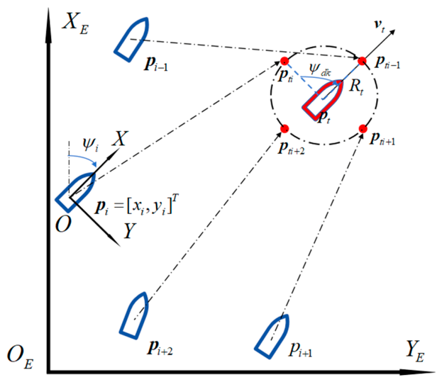
Figure 2.
Communication topology of the networked system.
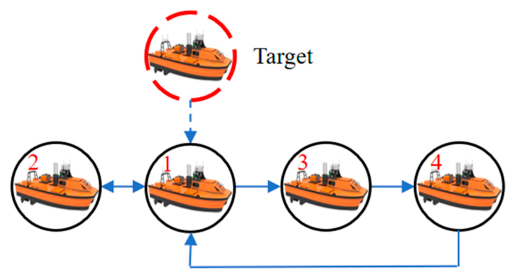
Figure 3.
USVs trajectory diagram under the SPT-TACC method.
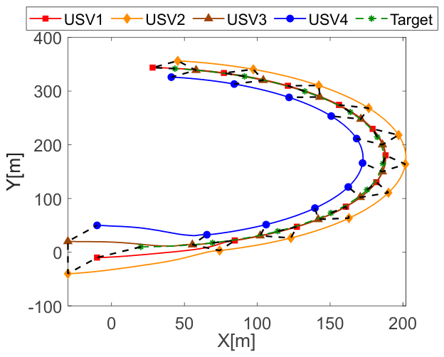
Figure 4.
kinematic errors between USVs and tracking points under the SPT-TACC method: (a) Position consistency errors; (b) Velocity consistency errors.
Figure 4.
kinematic errors between USVs and tracking points under the SPT-TACC method: (a) Position consistency errors; (b) Velocity consistency errors.
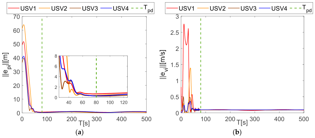
Figure 5.
kinematic errors between USVs and tracking points under the PT-TACC method: (a) Position consistency errors; (b) Velocity consistency errors.
Figure 5.
kinematic errors between USVs and tracking points under the PT-TACC method: (a) Position consistency errors; (b) Velocity consistency errors.
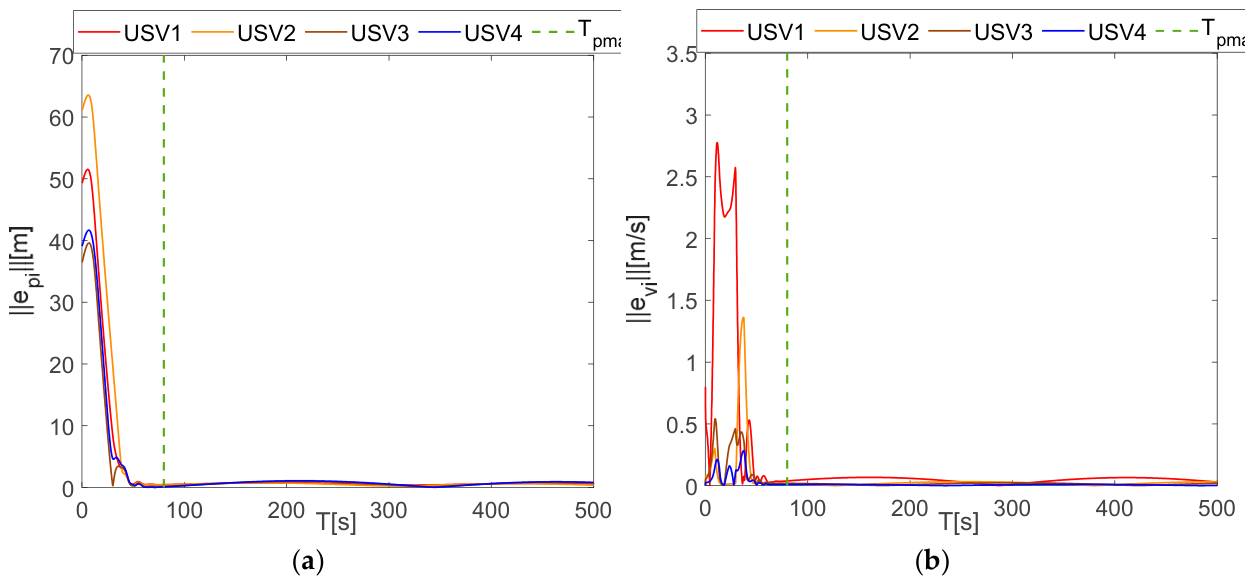
Figure 6.
Velocity tracking results under the SPT-TACC method.
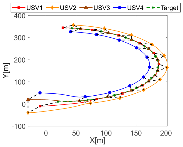
Figure 7.
kinetic error curves of USVs: (a) Kinetic errors under the SPT-TACC method; (b) Kinetic errors under the PT-TACC method.
Figure 7.
kinetic error curves of USVs: (a) Kinetic errors under the SPT-TACC method; (b) Kinetic errors under the PT-TACC method.
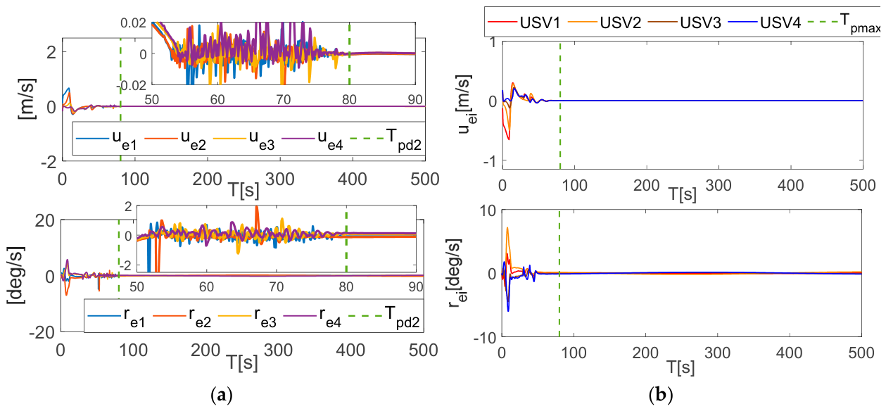
Figure 8.
Kinetic control outputs of 4 USVs.
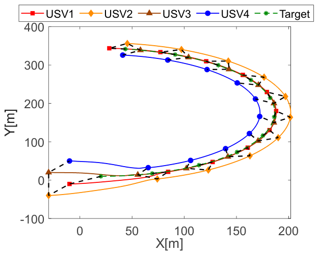

Table 1.
Main Simulation Parameters.
| Symbol | Value | Symbol | Value |
| 10 | 30 | ||
| 70 | 80 | ||
| 0.5 | 0.15 | ||
| 40 | |||
| 1 | 0.3 | ||
| 0.12 | 0.7 | ||
| 0.1 | 80 | ||
| 80 | 5 | ||
| 40 | |||
| 1.2 | 0.8 | ||
| 70 | 80 | ||
| 1 | 0.7 |
Table 2.
MSE value of cooperative kinematic error under the SPT-TACC method after 80s.
| USV1 | USV2 | USV3 | USV4 | Average value | |
| [m] | 0.5451 | 0.2755 | 0.4938 | 0.6340 | 0.4871 |
| [m/s] | 0.0076 | 0.0072 | 0.0074 | 0.0084 | 0.0077 |
Table 3.
MSE value of cooperative kinematic error under the PT-TACC method after 80s.
| USV1 | USV2 | USV3 | USV4 | Average value | |
| [m] | 0.5450 | 0.2754 | 0.4937 | 0.6341 | 0.4871 |
| [m/s] | 0.0075 | 0.0073 | 0.0075 | 0.0083 | 0.0077 |
Table 4.
MSE value of kinetic error under the SPT-TACC method before 80s.
| USV1 | USV2 | USV3 | USV4 | Average value | |
| [m] | 0.0418 | 0.0460 | 0.0044 | 0.0036 | 0.0165 |
| [°/s] |
Table 5.
MSE value of kinetic error under the PT-TACC method before 80s.
| USV1 | USV2 | USV3 | USV4 | Average value | |
| [m] | 0.0408 | 0.0164 | 0.0048 | 0.0038 | 0.0165 |
| [°/s] |
Table 6.
ITAE value of kinetic error under the SPT-TACC method.
| USV1 | USV2 | USV3 | USV4 | Average value | |
| [m] | |||||
| [°/s] | 29.86 | 161.68 | 49.25 | 82.63 | 80.86 |
Table 7.
ITAE value of kinetic error under the PT-TACC method.
| USV1 | USV2 | USV3 | USV4 | Average value | |
| [m] | |||||
| [°/s] | 22.21 | 129.34 | 43.08 | 75.53 | 67.54 |
Disclaimer/Publisher’s Note: The statements, opinions and data contained in all publications are solely those of the individual author(s) and contributor(s) and not of MDPI and/or the editor(s). MDPI and/or the editor(s) disclaim responsibility for any injury to people or property resulting from any ideas, methods, instructions or products referred to in the content. |
© 2026 by the authors. Licensee MDPI, Basel, Switzerland. This article is an open access article distributed under the terms and conditions of the Creative Commons Attribution (CC BY) license (http://creativecommons.org/licenses/by/4.0/).
Copyright: This open access article is published under a Creative Commons CC BY 4.0 license, which permit the free download, distribution, and reuse, provided that the author and preprint are cited in any reuse.