

Submitted:
10 September 2026
Posted:
14 September 2026
You are already at the latest version
Abstract
The parameters that determine practical applications oxide ferrimagnets are the values of saturation magnetizations and the magnitudes and signs of the magnetocrystalline anisotropy fields. Measuring magnetocrystalline anisotropy fields using ferromagnetic resonance (FMR) on single-crystal or textured polycrystalline hexaferrite samples is straightforward. However, these methods are not applicable for hexaferrite which typically synthesized as macroscopically magnetically isotropic polycrystalline or powder samples. This paper describes two methods to calculating the components of the permeability tensor of polycrystalline (or powder) hexaferrites in the independent grain approach. The proposed method is illustrated results of a FMR study of Y-type polycrystalline Ba2Ni2–xCuxFe12O22 (0.0 ≤ x ≤ 2.0) system, synthesized using a standard ceramic method. The measurements were performed on spherical samples in the frequency range of 37–50 GHz. The metod allows one to evaluate the magnitudes of the magnetocrystalline anisotropy fields and magnetomechanical ratios of both the target Y-phase and impurity phases. The phase composition estimates obtained from FMR data were compared with the results of X-ray phase analysis. It has been shown that up to a composition with x = 1.8, these materials are the ferroxplana-type hexaferrites. Hexaferrite Ba2Cu2Fe12O22 exhibits easy-axis type of the magnetocrystalline anisotropy.
Keywords:
polycrystalline hexaferrites
; ferromagnetic resonance
; magnetocrystalline anisotropy
; magnetomechanical ratio
1. Introduction
Oxide ferrimagnets with a hexagonal crystal structure (hexaferrites) are widely used in various fields of modern science and technology. The persistent interest of scientists and engineers to these materials is proven by the significant increase in the number of publications devoted to research on the physical properties and various aspects of their application, as noted in review papers [1,2,3,4].
Unlike ferrites with a spinel or garnet structure, hexaferrites exhibit high magnetocrystalline anisotropy (MCA) fields, as well as comparatively high saturation magnetization (MS) and Curie temperatures [5]. Based on their MCA type, hexaferrites are ranked into two main categories.
The first category includes magnetically hard materials (ferroxdures) with a positive anisotropy constant k1, large anisotropy field values (Hа1 = 2k1/MS), and the easy magnetization axis (EMA) type magnetic ordering aligned with the hexagonal c axis of the crystal. They are used for permanent magnets, as magnetic recording media and components in ultrahigh-frequency equipment. Ferroxdures include the simplest M-type hexaferrites BaxSr1–xFe12O19 (0.0 ≤ x ≤ 1.0) with a magnetoplumbite crystal structure. The production methods, magnetic properties, and applications of these materials are discussed in detail in [1,5] and in specialized reviews [6,7].
The second category consists of soft magnetic materials (ferroxplana) with a negative anisotropy constant k1 and easy magnetization plane (EMP) type of ordering. The six easy and intermediate magnetization directions for this group of materials are located in the basal plane of the crystal, perpendicular to the hexagonal c-axis. This category includes hexaferrites of more complex structural types: Y, W, Z, X, and U. The synthesis methods, crystallographic structure, and magnetic properties of ferroxplana are described in [1,5] and in a specialized review [8].
A distinctive feature of ferroxplana containing Co2+ ions is the presence of a sequence of spin-orientation phase transitions (SOPT) with decreasing temperature from the Curie point [5]. They exhibit EMA ordering near the Curie point as a rule. With decreasing temperature, a SOPT to magnetic ordering of the EMP type occurs through an intermediate phase of the easy magnetization cone (EMC) type. Further cooling leads to a SOPT from EMP to EMC. Typically, this SOPT occurs at temperatures below room temperature. In cobalt-containing W- and Z-type hexaferrites, the temperatures of these transitions were studied in detail in [9,10,11]. As a rule, the anisotropy field in the basal plane (HΦ) of ferroxplana is significantly smaller by approximately two orders of magnitude than the anisotropy field relative to the hexagonal axis (HΘ) [5]. Therefore, ferroxplana have higher permeability in the microwave range than EMA materials [5]. They are well suited for the fabrication of antenna substrates, as well as reciprocal and non-reciprocal microwave devices, with the ability to control their properties using an external magnetizing field. Furthermore, ferroxplana hold promise for the development of broadband radar-absorbing materials and coatings [12].
Thus, the knowledge of the magnitude and sign of the MCA fields and the saturation magnetization value is necessary for the targeted use of hexaferrites in a given frequency range. Determination MCA fields using ferromagnetic resonance (FMR) on single-crystal hexaferrite samples is straightforward [5,13,14]. However, hexaferrites are much more often manufactured and used in practice as polycrystals or powder fillers in composite materials.
Three methods are known for determining the magnitude of magnetocrystalline anisotropy fields from experiments on macroscopically isotropic polycrystalline or powder ferrimagnetic materials:
- the FMR method.
In the LAS method, the magnitude of the MCA field of uniaxial hexaferrites (Ha1) is estimated using the equation M(H)/MS =1– (1/15)(Ha1/H)2. It is obtained in the independent grain approach (IGA) under the assumption that the deviations of the magnetization vector from the direction of the magnetizing field (H) are small, i.e., in the case when H>>|Ha1|. Comparison of this equation with the "exact" solution within the IGA shows that an error in estimating |Ha1| of less than 5 % is achieved for magnetizing fields H ≥ 4.5|Ha1|.
The SPD method is based on measurement of the inflection point in the field dependence of magnetization M(H) of crystallites whose hard magnetization directions are close the direction of the magnetizing field. For uniaxial polycrystalline hexaferrites, this singularity appears at H=|Ha1| in the field dependence of the second derivative d2M(H)/dH2. Measurements are typically performed in pulsed magnetic field, and its maximum amplitude is H ≥ 2|Ha1|. The common disadvantages of these methods are:
- the need to use large magnetizing fields, significantly exceeding |Ha1|,
- the inability to determine the type of magnetic ordering of the material being studied (EMA or EMP), which is usually defined by the sign of the anisotropy constant k1.
The FMR method allows one to determine both the magnitude of the MCA fields and the type of magnetic ordering (EMA or EMP) of materials, as well as the magnitude of the effective magnetomechanical ratio γ = ge/(2mc). Here, g is the effective g-factor of the material under study, e is the electron charge, m is the electron mass, and c is the speed of light. This method is preferable for determining the MCA fields of materials with large anisotropy fields [10,21]. An undoubted advantage of the FMR method is its ability to measure magnetocrystalline anisotropy fields and estimate the content of individual phases in multiphase hexaferrites with magnetic ordering such as EMA [22] and EMP [23,24].
It is known that the optimal temperature ranges for the synthesis of hexaferrites of different structural types overlap, leading to the formation of impurity phases with a hexagonal crystal structure. Furthermore, the materials typically contain impurities of spinel phases with a low anisotropy field [1,5]. Therefore, the synthesis of single-phase samples is a challenging task, and it is of interest to analyze the MCA fields of the initial multiphase samples in order to select a material with the required MCA field value. After this, efforts can be concentrated on obtaining single-phase materials.
The results of a study of the structural, magnetic, and electromagnetic characteristics of planar hexaferrites of the Ba2Ni2–xCuxFe12O22 (Ni2–xCux–Y) system for compositions within range 0.0 ≤ x ≤ 2.0 are presented in [12]. The MCA fields of the Ni2–xCux–Y ferroxplana system for compositions 0.0 ≤ x ≤ 1.4 were determined using the FMR method in [24]. The measurements in this work were carried out using a waveguide method on powder samples placed in quartz tubes with an inner diameter of ≈ 0.7 mm. A magnetizing field was applied perpendicular to the tube axis, while an alternating magnetic field was applied along the sample axis. In this case, the contribution of the transverse demagnetization field of the cylindrical powder sample to the effective magnetic anisotropy field is difficult to control, what is the disadvantage of this experimental method.
The influence of demagnetizing fields of the sample can be eliminated when performing measurements on spherical samples. Therefore, the aim of this study is to measure the MCA fields of Ni2–xCux–Y hexaferrites system (0.0 ≤ x ≤ 2.0) using the FMR method on polycrystalline spherical samples with a diameter ≤ 1 mm in the frequency range of 36–50 GHz.
The second section of the paper presents the basic principles of constructing the FMR theory in polycrystalline hexaferrites in the independent grain approximation. The methods for calculating resonance curves of the polycrystalline samples are described. The third section is experimental and consists of two parts. The first part presents the results of X-ray phase analysis of the synthesized materials. The second part describes the method for processing the experimental FMR spectra of multiphase hexaferrite samples and presents the results of measurements of the MCA fields and the effective magnetomechanical ratios of the target Y-phase and impurity phases. The conclusion formulates the main results of the paper.
2. Materials and Methods
A polycrystalline (powder) material is a collection of single-crystal grains – crystallites, usually of irregular shape – separated by pores and magnetic and non-magnetic inclusions. The crystallographic axes of the grains are randomly oriented relative to each other. Thus, macroscopically, a polycrystals possesses all the properties of an isotropic medium. However, the experimentally observed FMR lines in polycrystals differ from the absorption curves of both isotropic materials and single crystals. First, the width of the FMR curve of polycrystals is much greater than that in single crystals of the same composition. Secondly, the shape of the resonance curve of a polycrystals differs significantly from the nearly Lorentzian FMR curve of a single crystal samples. It is typically asymmetric and may contain additional maxima and steps. The main causes of this distortion of the FMR curves of polycrystals are known:
- scatter in the directions of the MCA fields due to the random orientation of the crystallographic axes in different crystallites;
- demagnetizing fields arising from pores and nonmagnetic inclusions in polycrystals;
- variation in grain shape from crystallite to crystallite, leading to a distribution of demagnetizing fields within the grains;
- possible variation in the magnitude of the MCA fields in different grains.
Thus, to construct a theory of FMR in polycrystals, it is necessary to solve the problem of inhomogeneous, coupled magnetization oscillations in a large number of crystallites. This problem is extremely complex due to the irregular nature of the inhomogeneity’s in a polycrystals. Therefore, certain model concepts must be introduced. The most challenging aspect of constructing the theory is accounting for the interaction between magnetization oscillations in different crystallites, which is determined primarily by long-range magnetic dipole interactions. The currently developed models differ in role interpretation of this interaction. Moreover, the aforementioned sources of broadening are typically considered independently and are assumed to make an additive contribution to the parameters of the FMR resonance curve.
As noted earlier, hexaferrites, unlike spinel ferrites, have large anisotropy fields [5]. The relation |Ha| > 4πMS is generally satisfied for them and the magnetic dipole interaction between grains can be neglected. The theory of FMR in such materials is constructed within the approximation of non-interacting grains or independent grain approach in other words. The foundations of FMR theory in IGA were laid in the works of E. Schlömann for materials with cubic [25,26] and hexagonal [27] crystal structures. He solved the FMR problem analytically by expanding a system of transcendental equations into a series in a small parameter k = |Ha|/(ω/γ) << 1, which represents the ratio of the anisotropy field to the FMR field in an infinite isotropic medium which is equal to ω/γ. Here, ω = 2πf is the angular frequency and f is the linear frequency of the electromagnetic field.
E. Schlömann's approach to FMR theory in IGA approximation was generalized to the case of polycrystalline hexaferrites with arbitrary magnitude and sign of the MCA fields in article [10]. We assume that the polycrystalline sample consists of identical single-domain grains in the shape of an ellipsoid of revolution with a hexagonal MCA. The ellipsoid's axis of rotation coincides with the hexagonal c-axis. The crystallographic axes of the grains are randomly oriented relative to the direction of the magnetizing field. The density of the magnetic part of the free energy (U) consists of the contributions from the Zeeman energy (UZee), the energy of the demagnetizing fields (UM), and the energy of the magnetocrystalline anisotropy (UMCA). In a spherical coordinate system, it is written as follows:
Here, H is the magnitude of the external magnetizing field; Θ, Φ are its polar and azimuthal angles, relatively to the c-axis; ϑ, φ are the polar and azimuthal angles of the magnetization vector, relatively to the c-axis; ki is the i-th order magnetocrystalline anisotropy constant. N⊥, N‖ are the transverse and longitudinal demagnetization factors of an ellipsoidal particle, satisfying the normalization condition: 2N⊥+N‖=1. The anisotropy constant k1 describes the magnetocrystalline anisotropy relative to the hexagonal c-axis, the constants k1, k2, and k3 characterize the MCA relative to the basal plane, and the constant k4 characterizes the anisotropy in the basal plane of a monocrystalline grain.
In the first stage of solving the FMR problem in polycrystals, the equilibrium orientation angles of the magnetization vector (ϑ0(Θ, Φ), φ0(Θ, Φ)) and the magnitude of the resonant field H0(Θ, Φ) of an individual grain are calculated by solving a system of three transcendental equations. The first two equations determine the equilibrium orientation of the magnetization vector, and the third equation is the Smith–Suhl resonance condition:
Here, Hai = 2ki / MS (for i = 1, 2, 3), H’a1 = Ha1 – 4πMS(N‖– N⊥) , and HΦ = 36k4 / MS are the magnetocrystalline anisotropy fields, ω is the frequency of the applied electromagnetic field. The quantities Ω1, Ω2, Ω3 are defined as:
The system of Equation (2) is solved numerically at a fixed frequency ω by specifying the orientation of the magnetizing field over the angular ranges: 90° ≥ Θ ≥ 1°, 0° ≤ Φ ≤ 30°. These limits are determined by the symmetry of the MCA energy density. Practical experience in calculating resonance curves [10] has shown that varying the angles in 1° increments is sufficient. The calculations give a matrix of equilibrium angles ϑ0(Θ, Φ), φ0(Θ, Φ) and the resonant fields H0(Θ, Φ) for the given grid of magnetizing field orientations. The resonant field along the hexagonal axis (Θ = 0°, 0° ≤ Φ ≤30°) is calculated using the equation:
The imaginary part of the transverse diagonal component of the permeability tensor for a monocrystalline grain is calculated using the equation [14]:
Here, H is the magnitude of the applied external magnetic field, and α is dimensionless (dim.less) damping constant in the Landau-Lifshitz-Gilbert equation of motion for the monocrystalline grain. Compared to a single crystal, all unaccounted contributions to the additional broadening of the FMR curve in a polycrystal are incorporated by appropriately selecting the value of α when comparing theory with experiment.
The imaginary part of the permeability for a polycrystalline or powdered sample is proportional to the power absorbed by the sample at the FMR. It is calculated within the specified ranges of the magnetizing field (Hmin ≤ H ≤ Hmax) by averaging Eq. (5) over the angles Θ and Φ using the equation:
Here, cm is the concentration of the magnetic phase.
It should be noted that the approach proposed by E. Schlömann for analyzing the FMR curves of polycrystals, which is based on solving the system of Equation (2), has two main limitations. First, it is not applicable for analyzing FMR in single-domain particles with EMA ordering at frequencies below the natural ferromagnetic resonance (NFMR) frequency ωNFMR = γ H’a1. Second, this method does not allow for the calculating of FMR spectra during frequency sweeps at fixed magnetizing field values.
A method for calculating the components of the permeability tensor of uniaxial single-domain polycrystalline and powder materials within the IGA approximation, which is free from these drawbacks, was proposed in [28]. Crystals are considered uniaxial if their magnetocrystalline anisotropy in the basal plane is negligible compared to the magnetocrystalline anisotropy relative to the hexagonal axis, i.e., |HΘ| ≫ HΦ, where HΘ = H’a1 + Ha2 + Ha3. In uniaxial crystals, the magnetizing field and magnetization vectors are coplanar with the hexagonal c-axis. In this case, φ0 = Φ, and the starting point is the solution of the equation for the equilibrium polar angle of the magnetization vector ϑ0(H, Θ) for given values of the magnetizing field Hmin ≤ H ≤ Hmax and for angles Θ varying in a specified step from 0 to π/2:
The transverse diagonal component of the permeability tensor of the polycrystal obtained within the IGA, can be written as [28]:
The transverse diagonal components of the magnetic susceptibility tensor () for a monocrystalline grain in Eq. (8) are given by:
Here, ω0 is the resonance frequency of uniform precession and ωr is the relaxation frequency of a monocrystalline grain. The frequencies Ω1 and Ω2 are calculated using Eqs. (3) for φ0 = Φ and HΦ = 0. The Equations (7)–(9) can be used to calculate the FMR curve of a polycrystal both for a fixed magnetizing field with a frequency sweep, and for a variable magnetizing field within the range Hmin ≤ H ≤ Hmax at a given frequency ω.
Measurements of the MCA fields of Ni2–xCux–Y hexaferrite on powders samples (0.0 ≤ x ≤ 1.4) showed that the condition |HΘ| >> HΦ is satisfied for these materials [24]. Therefore, when comparing the experimental and calculated FMR curves to determine the MCA fields and magnetomechanical ratios in the following section, we used the FMR analysis technique based on Eqs. (7) – (9), which was developed for polycrystalline hexaferrites with uniaxial anisotropy.
3. Results and Discussion
3.1. Phase Composition of Ni2–xCux–Y Hexaferrite Samples
Polycrystalline Ba2Ni2–xCuxFe12O22 hexaferrite samples with 0.0 ≤ x ≤ 2.0 were synthesized using a standard two-stage ceramic technique. The resulting pellets were pre-annealed at 1150 °C for 6 hours, followed by a final annealing step at 1180 °C for 6 hours.
The phase composition of the hexaferrites was analyzed using a Shimadzu XRD 6000 X-ray diffractometer with Cu-Kα radiation at room temperature. The diffraction peaks were identified using the PDF4+ database and the Crystallographica Search-Match software package. Quantitative phase analysis of the diffraction patterns was performed using the PowderCell 2.4 software package. The results of the XRD phase analysis described in detail in [12,24] and presented in Table 1.
The second column of the Table 1 lists the content of the target Y-phase in the final synthesis products. The next three columns provide the concentrations of the identified impurity phases: the hexagonal M-phase (BaNiyCuzFe12-y-zO19), the spinel S-phase (NiyCuzFe3-y-zO4), and hematite α-Fe2O3. The concentrations y and z in these impurity phases were not determined in our experiments. As shown in the Table 1, the content of the target Y-phase in samples with different x values varies considerably, ranging from approximately 52 % to 97 %. All samples contain significant amounts of various impurity phases. This multiphase nature of the samples is expected to be clearly reflected in the measured FMR spectra. The designation "LA-phase" in Table 1 refers to phase (or phases) with low values of the MCA field estimated by the FMR method. The last column of the table shows the saturation magnetization per unit volume of the synthesized hexaferrite samples required for calculating the FMR curves. The magnetization values were calculated using the equation MS(x)=ρ(x)σS(x). The density ρ(x) of ferrites were calculated using the data in [5]. The values of specific saturation magnetization σS(x) were obtained by us in [12].
3.2. Phase Composition of Ni2–xCux–Y Hexaferrite Samples
The FMR absorption curves are proportional to the microwave power absorbed by the sample during resonance, which is, in turn, proportional to the imaginary part of the sample's permeability. To determine the MCA fields (H’a1, HΘ) and the magnetomechanical ratios (γ), the experimental FMR curves were measured using a waveguide transmission method at fixed frequencies in the range of 36 to 50 GHz with a sweep of the magnetizing field. These curves were then compared with the theoretical µ´´poli(H, ω) dependences calculated within the IGA. The method for processing the FMR spectra is described in detail in [10,21,23]. The procedure is as follows.
First, by varying the parameters H’a1, HΘ and γ, a match is achieved between the position of the maxima in the calculated and experimental FMR curves at several frequencies within the selected range. Next, by adjusting the damping constant α of the crystallite, which governs the linewidth and intensity of its resonance curve, a match between the shapes of the calculated and experimental resonance curves is ensured. According to Eqs. (5) and (9), the area under the µ´´poli(H, ω) curve is proportional to the saturation magnetization of the sample material.
When constructing the calculated FMR curves for the Y-phase, the MS values listed in Table 1 were used; these obtained for the Ni2–xCux–Y system based on data from [12]. Since estimating the MS values for the impurity phases from our data is difficult, a saturation magnetization of 380 G was used for the M-phase, corresponding BaFe12O19, and a value of 480 G was used for the S-phase, corresponding to magnetite (Fe₃O₄) [5]. The contribution of the antiferromagnetic hematite phase to the FMR absorption was neglected due to its expected insignificance.
Figure 1 shows the experimental and calculated FMR curves at a frequency of 36 GHz for Ni2–xCux–Y hexaferrites with compositions x = 0.0, 0.4, 0.8, 1.2, 1.6, and 2.0. The markers represent the experimental data, and the solid lines represent the calculated fits. It is known that most Y-type hexaferrites exhibit EMP magnetic ordering with a large negative anisotropy field HΘ [5]. The contribution of the Y-phase with EMP (curves 1 for compositions with x ≤ 1.8) to the total absorption manifests as broad, asymmetric resonance curves with a manifested maximum at fields lower than ω/γ and a step on the high-field side. In contrast, resonance curve 1 for the Cu2–Y hexaferrite (x = 2.0) exhibits two well-defined maxima, which is characteristic of FMR curves for materials with EMA ordering (H’a1 > 0). The partial contributions from the M-phase to the total absorption have a similar shape for the samples with x = 0.8 and 1.6. The FMR curves for all compositions, except x = 1.6, show an additional resonance feature (curves 2). This feature resembles a symmetric Lorentzian line, with a resonant field close to Hres = ω/γ = 12.85 kOe. This value corresponds to the resonance field of a spherical sample of an isotropic ferromagnetic material at frequency equal 36 GHz assuming a magnetomechanical ratio of γ/2π = 2.8 MHz/Oe (which corresponds to a g-factor of 2.0).
Therefore, it can be inferred that this contribution to the total absorption originates from the spinel S-phase, which has a small MCA field, and possibly from other impurity phases, provided their particles are small and are in a superparamagnetic state. We refer to this contribution as the low-anisotropy (LA) phase. The combined resonance curves for the three phases were constructed by adjusting the concentrations of the partial contributions from each phase to achieve the closest possible match with the experimental curves. The phase concentrations derived from the FMR data are presented in the corresponding columns of Table 1. Since the true magnetization values of the individual phases are not precisely known, these estimates are approximate. Nevertheless, regarding the content of the target Y-phase, they show good correlation with the X-ray phase analysis data, with the exception of the sample with x = 1.4.
The values of the MCA fields, magnetomechanical ratios, and dimensionless damping constant of the Y-, LA-, and M-phases, which were used to calculate the partial FMR curves in Figure 1, are presented in Table 2. The calculation errors of these values estimated during the fitting procedures presented in the Table 2 were: ± 0.1 kOe for anisotropy fields; ± 0.01 GHz/kOe for magnetomechanical ratios; < ± 0.005 for damping constants.
Table 2 shows that Ni2–xCux–Y hexaferrites exhibit EMP type magnetocrystalline anisotropy in the concentrations range 0.0 ≤ x ≤ 1.8, with the anisotropy field HΘ showing a tendency to decrease with increasing x. In contrast, the Cu2–Y hexaferrite (x = 2.0) exhibits EMA type anisotropy. A similar result for this material was reported in [29]. The anisotropy field for the Ni2-Y hexaferrite (x = 0.0) is close to the value of –14 kOe given in [5]. The estimated Ha values for the LA-phase are also consistent with the anisotropy fields of spinel ferrites reported in [5], such as Fe3O4 (–460 Oe), NiFe2O4 (–460 Oe), and CuFe2O4 (–889 Oe). The magnetocrystalline anisotropy fields of the impurity M-phases are significantly smaller than the 17 kOe value for pure barium hexaferrite (BaFe12O19) [5]. The magnetomechanical ratios for both the highly anisotropic and low-anisotropy phases are close to the value for a free electron spin (2.8 GHz/kOe). It should be noted that the undoubted advantage of the FMR method is the ability to estimate the contribution of the higher-order MCA fields (Ha2+ Ha3) to the HΘ anisotropy field.
It is of interest to compare the values of the MCA fields HΘ obtained in this work on spherical samples with the results of our HΘ measurements on cylindrical powder samples in [24]. The results are presented in Table 3.
The Table 3 shows that, with the exception of the sample with x = 1.4, measurements on cylindrical powder samples yield an anisotropy field HΘ that is, on average, overestimated by 0.4 kOe. This fact is explained by the contribution of the anisotropy of the cylindrical sample's shape to the resonant field.
4. Conclusions
The theoretical part of the paper examines two approaches to describing the FMR in polycrystalline and powder hexaferrites in the independent grain approximation. The first approach is applicable to materials with a non-zero MCA field in the basal plane HΦ, but fails at frequencies lower than the NFMR frequency. The second approach is developed for uniaxial materials with HΦ ≈ 0, but is applicable to analyzing magnetization oscillations in polycrystalline materials at arbitrary (but non-zero) magnetizing fields and frequencies.
In this study, the magnetocrystalline anisotropy fields and magnetomechanical ratios of polycrystalline hexaferrites in the Ba2Ni2–xCuxFe12O22 system were determined for Cu2+ ion concentrations in the range 0.0 ≤ x ≤ 2.0. This was achieved by comparing experimental FMR spectra with theoretical spectra calculated within the independent grain approximation. Measurements were carried out on samples of spherical shape in the frequency range from 36 GHz to 50 GHz.
Since specific synthesis regimes for obtaining single-phase samples were not developed, the synthesized materials were multiphase. According to X-ray diffraction data, in addition to the target Ni2–xCux–Y phase, the samples contained impurity phases, including a spinel ferrite, hematite, and the hexagonal Ba-M phase. It was demonstrated that FMR studies of multiphase hexaferrite samples enable the evaluation of the MCA fields, magnetomechanical ratios, and relative concentrations of the constituent phases.
Ni2–xCux–Y hexaferrites exhibit an EMP-type magnetic ordering up to the composition with x = 1.8. With increasing substitution of Cu2+ ions for Ni2+ ions, the MCA field relative to the basal plane HΘ exhibits a decreasing trend. Cu2–Y hexaferrite exhibits an EMA-type of magnetic ordering.
Author Contributions
Conceptualization, V.A.Z.; data curation, V.A.Z., D.V.W., O.A.D., K.V.K. and R.S.S.; formal analysis, V.A.Z., D.V.W. and O.A.D.; funding acquisition, V.A.Z.; investigation, V.A.Z., D.V.W., O.A.D., K.V.K. and R.S.S.; methodology, V.A.Z., D.V.W.; project administration, V.A.Z.; validation, V.A.Z., D.V.W., O.A.D. and K.V.K.; writing -original draft, V.A.Z., D.V.W.; writing - review & editing, D.V.W., O.A.D., K.V.K.; visualization, K.V.K., R.S.S.
Funding
This work was supported by the Russian Science Foundation [grant number 26-19-00908, https://rscf.ru/en/project/26-19-00908/].
Data Availability Statement
Not applicable.
Acknowledgments
The magnetic measurements of the hexaferrites were performed using the equipment of the TSU Center for Radiophysical Measurements, a Collective Use Center.
Conflicts of Interest
The authors declare no conflicts of interest.
Abbreviations
The following abbreviations are used in this manuscript:
| EMA | Easy magnetization axis |
| EMC | Easy magnetization cones |
| EMP | Easy magnetization plane |
| FMR | Ferromagnetic resonance |
| IGA | Independent grain approach |
| LA | Low anisotropy |
| LAS | Law approach to saturation |
| MCA | Magnetocrystalline anisotropy |
| NFMR | Natural ferromagnetic resonance |
| SPD | Singular point detection |
References
- Pullar, R.C. Hexagonal ferrites: A review of the synthesis, properties and applications of hexaferrite ceramics. Prog. Mater. Sci. 2012, 57, 1191–1334. [Google Scholar] [CrossRef]
- Koledintseva, M.Y.; Khanamirov, A.E.; Kitaitsev, A.A. Advances in Engineering and Applications of Hexagonal Ferrites in Russia. In Advances in Ceramics – Electric and Magnetic Ceramics, Bioceramics, Ceramics and Environment; Sikalidis, С., Ed.; InTechOpen, London, 2011; pp. 61–86. [Google Scholar]
- Harris, V.G.; Geiler, A.; Chen, Y.; et al. Recent advances in processing and applications of microwave ferrites. J. Magn. Magn. Mater. 2009, 321, 2035–2047. [Google Scholar] [CrossRef]
- Harris, V.G. Modern Microwave Ferrites. IEEE Trans. Magn. 2012, 48, 1075–1104. [Google Scholar] [CrossRef]
- Smit, J.; Wijn, H.P.J. Ferrites: Physical Properties of Ferrimagnetic Oxides in Relation to Their Technical Applications; Philips Technical Library: Eindhoven, 1959. [Google Scholar]
- Pereira, F.M.M.; Sombra, A.S.B. A review on BaxSr1-xFe12O19 hexagonal ferrites for use in electronic devices. Solid State Phenom. 2013, 202, 1–64. [Google Scholar] [CrossRef]
- Singh, V.P.; Jasrotia, R.; Kumar, R.; et al. A Current Review on the Synthesis and Magnetic Properties of M-Type Hexaferrites Material. World J. Condens Matter Phys. 2018, 8, 36–61. [Google Scholar]
- Sugimoto, M. Chapter 6 Properties of Ferroxplana-Type Hexagonal Ferrites. Handb. Ferromagn. Mater. 1982, 3, 393–440. [Google Scholar] [CrossRef]
- Naiden, E.P.; Maltsev, V.I.; Ryabtsev, G.I. Magnetic Structure and Spin-Orientational Transitions of Hexaferrites of the BaCo2-xZnxFe16O27 System. Phys. Status Solidi A 1990, 120, 209–220. [Google Scholar] [CrossRef]
- Zhuravlev, V.A.; Zhuravlev, A.V.; Atamasov, V.V.; Malenko, G.I. Magnetocrystalline Anisotropy and Spin-Orientation Phase Transitions of Co2Z Hexaferrite Doped by Ti4+ and Zn2+ Ions. Russ. Phys. J. 2020, 62, 1926–1936. [Google Scholar]
- Nakajima, H.; Kawase, H.; Kurushima, K.; et al. Observation of magnetic domain and bubble structures in magnetoelectric Sr3Co2Fe24O41. Phys. Rev. B 2017, 96, 024431. [Google Scholar] [CrossRef]
- Zhuravlev, V.A.; Wagner, D.V.; Dotsenko, O.A.; et al. Static and Dynamic Magnetic Properties of Polycrystalline Hexaferrites of the Ba2Ni2-xCuxFe12O22 System. Electronics 2022, 11, 2759. [Google Scholar] [CrossRef]
- Gurevich, A.G.; Sanina, V.A.; Golovenchic, Е.Е.; Starobinets, S.S. Resonance in Magnetically Ordered Crystals with Anisotropic g Factors. J. Appl. Phys. 1969, 40, 1512–1517. [Google Scholar] [CrossRef]
- Gurevich, A.G.; Melkov, G.A. Magnetization Oscillations and Waves, first ed.; CRC Press: London, 1996. [Google Scholar]
- Grossinger, R. A Critical Examination of the Law of Approach to Saturation I. Fit Procedure. Phys. Status Solidi A 1981, 66, 665–674. [Google Scholar] [CrossRef]
- Golubenko, Z.V.; Ol’khovik, L.P.; Popkov, Y.A.; et al. Magnetic Anisotropy of a System of Nanocrystalline BaO-6Fe2O3 particles. Phys. Solid State 1998, 40, 1718–1720. [Google Scholar] [CrossRef]
- Grossinger, R. Correlation between the inhomogeneity and the magnetic anisotropy in polycrystalline ferromagnetic materials. J. Magn. Magn. Mater. 1982, 28, 137–142. [Google Scholar] [CrossRef]
- Asti, G.; Rinaldi, S. Singular Points in the Magnetization Curve of a Polycrystalline Ferromagnet. J. Appl. Phys. 1974, 45, 3600–3610. [Google Scholar] [CrossRef]
- Grossinger, R. Generation, Measuring Technique and Application of Pulsed Fields. J. Alloys Compd. 2004, 369, 5–9. [Google Scholar] [CrossRef]
- Kreslin, V.Y.; Naiden, E.P. Automatic complex for a study of the characteristics of hard magnetic materials. In Instrum; Exp. Tech., 2002; Volume 45, pp. 55–57. [Google Scholar]
- Zhuravlev, V.A.; Itin, V.I.; Minin, R.V.; et al. Influence of Different Organic Fuels on the Phase Composition, Structure Parameters and Magnetic Properties of Hexaferrites BaFe12O19 Synthesized by the Sol-Gel Combustion. J. Alloys Compd. 2019, 771, 686–698. [Google Scholar] [CrossRef]
- Zhuravlev, V.A.; Minin, R.V.; Itin, V.I.; et al. Study of the magnetic anisotropy of the multiphase samples of the ferrimagnets with hexagonal crystal structure by the method of ferromagnetic resonance. IOP Conf. Ser. Mater. Sci. Eng. 2017, 168, 012081. [Google Scholar] [CrossRef]
- Zhuravlev, V.A.; Naiden, E.P. Dependence of the structural parameters and magnetic properties of nanoscale powders of hexaferrite Zn2Y on the mechanical activation regimes. Phys. Solid State 2009, 51, 327–333. [Google Scholar] [CrossRef]
- Zhuravlev, V.A.; Suslyaev, V.I.; Lopushnvak, Y.M.; et al. Magnetocrystalline Anisotropy of the Multiphase Samples of the Hexaferrites Ba2Ni2-xCuxFe12O22 Studied by the Ferromagnetic Resonance Method. IOP Conf. Ser. Mater. Sci. Eng. 2019, 479, 012073. [Google Scholar] [CrossRef]
- Schlömann, E. Ferromagnetic Resonance in Polycrystalline Ferrites with Large Anisotropy – I: General Theory and Application to Cubic Materials with a Negative Anisotropy Constant. J. Phys. Chem. Solids 1958, 6, 257–266. [Google Scholar]
- Schlömann, E. Ferromagnetic Resonance in Polycrystals. J. Phys. Radium 1959, 20, 327–332. [Google Scholar] [CrossRef]
- Schlömann, E.; Jones, R.V. Ferromagnetic resonance in polycrystalline ferrites with hexagonal crystal structure. J. Appl. Phys. 1959, 30, 177S–178S. [Google Scholar] [CrossRef]
- Zhuravlev, V.A.; Meshcheryakov, V.A. Magnetic Susceptibility Tensor of Anisotropic Ferromagnetic Magnetized Media. Russ. Phys. J. 2014, 56, 1387–1397. [Google Scholar] [CrossRef]
- Castelliz, L.M.; Kim, K.M.; Boucher, P.S. Preparation, stability range and high frequency permeability of some ferroxplana compounds. J. Can. Ceram. Soc. 1969, 38, 57–62. [Google Scholar]
Figure 1.
FMR curves of Ni2–xCux–Y hexaferrites with compositions x = 0.0, 0.4, 0.8, 1.2, 1.6, and 2.0 at a frequency of 36 GHz. The compositions are indicated in the figures. The markers represent experimental data, and the lines represent the calculated curves. The partial contributions to the total absorption are denoted as follows: 1 – Y-phase; 2 – LA-phase; 3 – total resonance curve; 4 – M-phase.
Figure 1.
FMR curves of Ni2–xCux–Y hexaferrites with compositions x = 0.0, 0.4, 0.8, 1.2, 1.6, and 2.0 at a frequency of 36 GHz. The compositions are indicated in the figures. The markers represent experimental data, and the lines represent the calculated curves. The partial contributions to the total absorption are denoted as follows: 1 – Y-phase; 2 – LA-phase; 3 – total resonance curve; 4 – M-phase.
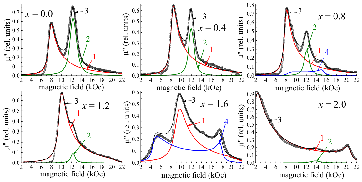

Table 1.
Phase composition of the synthesized Ni2–xCux–Y hexaferrites according to XRD data and estimated by the FMR method.
Table 1.
Phase composition of the synthesized Ni2–xCux–Y hexaferrites according to XRD data and estimated by the FMR method.
| Concent-ration | Results of X-ray phase analysis [12,24], % |
Phase composition according to FMR data, % |
MS, G | |||||
| x | Y-phase | M-phase | S-phase | α-Fe2O3 | Y-phase | M-phase | LA-phase | |
| 0.0 | 86.6 | - | 4.5 | 8.9 | 84.5 | - | 15.5 | 127.4 |
| 0.2 | 72.7 | 14.0 | 9.3 | 4.0 | 86.7 | - | 13.3 | 136.2 |
| 0.4 | 83.0 | 6.6 | 8.9 | 1.5 | 91.5 | - | 8.5 | 134.7 |
| 0.6 | 97.2 | - | - | 2.8 | 95.9 | - | 4.1 | 130.5 |
| 0.8 | 61.1 | 20.0 | 6.9 | 12.0 | 89.0 | 5.5 | 5.5 | 151.8 |
| 1.0 | 83.0 | 3.0 | 11.0 | 3.0 | 94.5 | - | 5.5 | 148.7 |
| 1.2 | 85.0 | 4.7 | 8.1 | 2.2 | 98.4 | - | 1.6 | 138.5 |
| 1.4 | 52.5 | - | 9.2 | 38.3 | 97.5 | - | 2.5 | 139.1 |
| 1.6 | 74.0 | 12.0 | 7.0 | 7.0 | 76.0 | 24.0 | - | 172.5 |
| 1.8 | 54.9 | 24.4 | 7.2 | 13.5 | 72.0 | 24.0 | 4.0 | 191.7 |
| 2.0 | 92.4 | 6.1 | - | 1.5 | 99.0 | - | 1.0 | 225.6 |
Table 2.
Magnetic parameters of the Y-, LA- and M- phases of synthesized materials determined from FMR experiments.
Table 2.
Magnetic parameters of the Y-, LA- and M- phases of synthesized materials determined from FMR experiments.
| x | 0.0 | 0.2 | 0.4 | 0.6 | 0.8 | 1.0 | 1.2 | 1.4 | 1.6 | 1.8 | 2.0 |
| Y-phase | |||||||||||
| HΘ, kOe | -12.5 | -12.4 | -10.7 | -12.5 | -11.6 | -10.6 | -6.5 | -7.6 | -8.2 | -9.2 | 12.5 |
| H’a1,kOe | -12.5 | -12.4 | -10.7 | -12.5 | -11.6 | -10.6 | -8.0 | -8.6 | -8.2 | -9.2 | 11.0 |
| Ha2+ Ha3, kOe | 0.0 | 0.0 | 0.0 | 0.0 | 0.0 | 0.0 | 1.5 | 1.0 | 0.0 | 0.0 | 1.5 |
| γ/2π, GHz/kOe | 2.88 | 2.88 | 2.88 | 2.88 | 2.89 | 2.89 | 2.85 | 2.84 | 2.82 | 2.85 | 2.80 |
| α, dim.less units | 0.04 | 0.04 | 0.04 | 0.03 | 0.04 | 0.04 | 0.05 | 0.04 | 0.08 | 0.05 | 0.05 |
| LA-phase | |||||||||||
| Ha, kOe | -0.7 | -0.6 | -0.6 | -0.5 | -0.5 | -0.3 | -0.3 | -0.2 | - | -0.5 | -0.5 |
| γ/2π, GHz/kOe | 2.91 | 2.95 | 2.99 | 3.02 | 2.97 | 2.89 | 2.93 | 2.84 | - | 2.95 | 2.60 |
| α, dim.less units | 0.05 | 0.05 | 0.04 | 0.03 | 0.04 | 0.07 | 0.04 | 0.05 | - | 0.09 | 0.08 |
| M-phase | |||||||||||
| H’a1,kOe | - | - | - | - | 4.5 | - | - | - | 8.5 | 7.3 | - |
| γ/2π, GHz/kOe | - | - | - | - | 2.80 | - | - | - | 2.78 | 2.80 | - |
| α, dim.less units | - | - | - | - | 0.04 | - | - | - | 0.04 | 0.03 | - |
Table 3.
Comparison of the values of the anisotropy fields HΘ.
| Concentration, x | 0.0 | 0.2 | 0.4 | 1.0 | 1.2 | 1.4 |
| HΘ, kOe (this work) | -12.5 | -12.4 | -10.7 | -10.6 | -6.5 | -7.6 |
| HΘ, kOe ([24]) | -12.9 | -12.6 | -11.0 | -11.3 | -7.1 | -7.5 |
| ΔHΘ, kOe | -0.4 | -0.2 | -0.3 | -0.7 | -0.6 | 0.1 |
Disclaimer/Publisher’s Note: The statements, opinions and data contained in all publications are solely those of the individual author(s) and contributor(s) and not of MDPI and/or the editor(s). MDPI and/or the editor(s) disclaim responsibility for any injury to people or property resulting from any ideas, methods, instructions or products referred to in the content. |
© 2026 by the authors. Licensee MDPI, Basel, Switzerland. This article is an open access article distributed under the terms and conditions of the Creative Commons Attribution (CC BY) license.
Copyright: This open access article is published under a Creative Commons CC BY 4.0 license, which permit the free download, distribution, and reuse, provided that the author and preprint are cited in any reuse.