

Submitted:
09 September 2026
Posted:
11 September 2026
You are already at the latest version
Abstract
Sequence models for RNA-binding proteins (RBPs) are evaluated against constructed negativewindows, but the influence of negative selection on estimated model contribution is poorlycharacterised. I compared GC-matched, dinucleotide-matched and bias-aware negatives across 94ENCODE eCLIP datasets, using the same source peaks and holding the model class, chromosome-blocked folds and estimator fixed. Contribution was defined as incremental AUROC over a19-feature composition baseline. For a 4-mer model, contribution varied 4.84-fold across protocols (95% CI 3.98–5.81) withthe primary cross-fitted estimator and 5.42-fold (4.43–6.58) with the conventional two-stageestimator. Two-stage spans ranged from 3.7- to 7.4-fold across the 4-mer, a convolutional neuralnetwork and SpliceBERT. Replacing GC-matched with dinucleotide-matched negatives reducedthe 4-mer AUROC from 0.798 to 0.688 in all 94 datasets, while increasing its contribution from0.027 to 0.066 in 88 datasets. The conventional estimator also produced a positive null contribution of +0.011 to +0.014for a 2-mer model whose features were contained in the baseline. Cross-fitting the scorecovariate reduced this floor by at least 95% in every protocol. In 135 held-out datasets from anindependently constructed benchmark, the two negative sets produced a 1.66-fold cross-fittedspan (95% CI 1.40–1.98), or 1.67-fold (1.40–2.00) after chromosome-blocked refolding. Protocoldependence replicated, whereas the inverse relation between apparent difficulty and contributiondid not.Incremental performance therefore depends on both the negative-set protocol and the baselineused to define it. I recommend cross-fitting score covariates, reporting composition-only per-formance under the same protocol, and avoiding direct comparisons of contributions estimatedunder different negative-set constructions.
Keywords:
RNA-binding proteins
; eCLIP
; benchmarking
; negative-set construction
; sequence composition
; incremental value
; AUROC
1. Introduction
Sequence models of RNA-binding protein (RBP) occupancy are commonly evaluated by the area under the receiver operating characteristic curve (AUROC) on held-out sequence windows. Positive windows are defined by crosslinking assays such as eCLIP [2,3]; negative windows must instead be constructed. Typical choices include unbound regions from the same transcripts [19], composition-matched genomic windows [6], and sites bound by other RBPs [4]. This choice determines the discrimination problem presented to the model, but it is often described only briefly.
The consequences can be substantial. Horlacher et al. [4] evaluated eleven RBP-prediction methods across hundreds of CLIP-seq experiments and showed that apparent performance depended on the negative-set definition. They proposed a bias-aware protocol in which sites bound by other RBPs serve as negatives, thereby reducing some of the compositional and accessibility differences between bound sites and genomic background. Related sensitivity has been observed in transcription-factor binding prediction: models trained with dinucleotide-shuffled negatives transferred less effectively to held-out high-quality data than models trained with genomic negatives [5]. More generally, evaluation-set construction can inflate apparent accuracy, alter method rankings and change the interpretation of genomic prediction models [7,8,10,11].
Raw AUROC combines two quantities: the signal captured by a model and the difficulty of the classification task defined by the benchmark. Uniform genomic negatives, for example, may differ markedly from crosslinked positives in nucleotide composition. A classifier can then achieve a high AUROC by exploiting composition alone. GC matching reduces one component of this difference, but GC content constrains only one linear combination of the sixteen dinucleotide frequencies. The remaining compositional degrees of freedom may still support substantial discrimination. Similar dependence of incremental performance on baseline strength has been described outside genomics [15].
I therefore distinguish a model’s apparent AUROC from its contribution beyond an explicit composition baseline. Apparent AUROC is the performance reported under a particular negative-set protocol. The nested contribution is the difference between two pooled out-of-fold AUROCs: one from a logistic model containing composition features and the sequence model’s score, and one from the same composition features alone. Both models are fitted on the same observations and folds. The primary baseline contains mono- and dinucleotide frequencies and sequence entropy, represented by 19 columns after removing redundant frequency levels. Because the resulting contribution depends on the baseline used to define it, I also evaluate higher-order composition models.
This analysis uses 94 ENCODE eCLIP datasets and three negative-set protocols: GC-matched genomic windows, dinucleotide-matched genomic windows, and a bias-aware set drawn from sites of other RBPs assayed in the same cell line. The protocols differ not only in composition matching but also in transcript-region constraints and transcriptional status. Across protocols I use the same source peaks and hold the model class and hyperparameters, chromosome-blocked fold assignment and estimator implementation fixed; the sequence model and composition baseline are refitted within each protocol. I examine a 4-mer logistic regression, a 7089-parameter convolutional neural network and a fully fine-tuned 19.78 M-parameter SpliceBERT model [20].
Within the study panel, stricter composition matching lowered apparent AUROC while increasing the estimated contribution beyond composition. The magnitude of this contribution varied several-fold across protocols and was comparable to the variation produced by changing model class. The dependence persisted across alternative performance measures and baseline orders, although its magnitude changed. I further identified a positive null floor in the conventional two-stage estimator and showed that cross-fitting the score covariate largely removed it. Finally, an analysis of 135 held-out datasets from Horlacher et al. [4] reproduced the protocol dependence but not the inverse relation between apparent difficulty and contribution.
Together, these results motivate three reporting practices: evaluate the composition baseline under the same protocol as the sequence model, cross-fit score covariates when estimating incremental performance, and avoid comparing contributions obtained under different negative-set constructions. The aim is not to identify a universally preferred negative set, but to make the scientific question posed by each benchmark explicit and its measurements interpretable.
2. Materials and Methods
2.1. Panel Selection
Candidate experiments were every released ENCODE eCLIP experiment in K562 and HepG2 (139 and 105 respectively). Where a protein had several peak files I took the one with the most biological replicates, breaking ties by ENCODE’s preferred_default flag, and required output_type=peaks, assembly=GRCh38, status=released and file_format=bed. Every candidate was preprocessed under both composition-matching protocols; datasets retaining at least 400 out-of-fold scored pairs were eligible.
The study panel was then defined once by the dinucleotide arm, which is the stricter control: the 189 eligible datasets were sorted by pair count with a stable sort and every second one retained, giving 95 datasets over 79 proteins. The set was halved rather than taken whole because the sweep trains three model classes over five folds and three protocols, and the full eligible set did not fit the compute budget the retained panel already consumes. Given that a reduction was necessary, I sampled systematically by rank rather than taking the largest N. AUROC correlates with dataset size in these data: negligibly for the composition baseline (Pearson r on of in the GC arm) but strongly for the models, reaching for SpliceBERT under dinucleotide matching. A size-truncated panel would therefore confound panel membership with the measured quantity. The retained panel spans the 0th to 99th percentile of the candidate size distribution. Of the 95, 94 also cleared the floor in the GC arm and constitute the paired panel used for every three-protocol result, giving 282 protocol-dataset cells. The 95th carries no three-protocol result, since it did not clear the out-of-fold pair floor in the GC arm, and every analysis reported here is on the 94. Panel membership was written once to a manifest that every downstream stage reads. Supplementary Table S1 lists every dataset with its ENCFF file and ENCSR experiment accession.
Sixteen proteins are assayed in both cell lines and contribute two datasets each, fifteen of them in the paired panel. All headline intervals therefore resample proteins rather than datasets.
2.2. Windows
Positive windows are 101 nt centred on the midpoint of each peak interval. Peak width and the significance columns are unused: I applied no further p-value, q-value or fold-change filter, because ENCODE’s released peaks files are already thresholded and across the 95 files the minimum log2 fold-enrichment is 3.0000 and the minimum is 3.0003, which are the criteria of Van Nostrand et al. [3]; 91.7% of the 463,091 peaks carry ENCODE’s IDR label. The positive set is therefore every peak ENCODE called and no weaker ones. Minus-strand windows are reverse-complemented and transcribed to RNA; every sequence is the strand the protein sees. Windows containing an ambiguous base, falling outside the assembly, duplicating an existing window by start coordinate, or carrying no region annotation are dropped and counted. Analysis is restricted to chr1 to chr22 and chrX; chrY and all scaffolds and alternates are excluded.
Region class is assigned from GENCODE v45 [9] as the first of (5′UTR, 3′UTR, CDS, non-coding exon, intron) whose interval set contains the window midpoint. Region intervals were built from all transcripts with no gene-type filter and merged, with strand disregarded at this step; introns were computed as the gaps between consecutive exons. GTF 1-based inclusive coordinates are converted to 0-based half-open.
2.3. The Three Negative-Set Protocols
Each protocol produces one negative per positive. All three use a single random stream seeded at 7 per protein.
GC-matched.
Candidates are windows of the same region class on the same chromosome, at least 500 nt from any peak of the target protein, drawn with probability proportional to the length of each free interval. A candidate is accepted if its GC content is within 0.05 of the positive’s. The matcher relaxes: after 25 unsuccessful draws the tolerance doubles to 0.10, and if 40 draws fail the best candidate seen is accepted provided it is within three times the nominal tolerance, that is 0.15. Only the target protein’s own peaks are excluded, and a GC-matched or dinucleotide-matched negative may be another protein’s binding site. The negative inherits the positive’s strand label; the consequences are quantified in the Results.
Dinucleotide-matched.
Positives are grouped by region and chromosome, and for each group a candidate pool of windows is sampled from the same free intervals the GC matcher draws on: same region class, same chromosome, and at least 500 nt from any peak of the target protein, the exclusion applied through the same code path and the same configured distance. The two composition-matched protocols therefore share one candidate universe and differ only in the statistic they match on. For each positive the nearest unused candidate is assigned greedily under the distance over the sixteen dinucleotide counts, searched with a k-d tree over the forty nearest neighbours. The distance is over counts, not frequencies, because integer distances are exactly representable, and each candidate carries an additional tiebreak column that increases strictly with genomic position and is bounded below 0.5, so it can never reorder candidates whose integer distances differ but resolves exact ties by position. Without both devices the choice among tied candidates depends on the floating-point behaviour of the k-d tree implementation and a different negative is selected for about 8% of pairs between CPU architectures. Assignment is greedy, not optimal; achieved distances are reported so the quality of the approximation is visible. Used coordinates are tracked across all groups, because one interval can be annotated as both a non-coding exon and a 3′UTR and so appear in two region pools. No maximum distance is imposed.
Bias-aware (other RBPs’ sites).
Following Horlacher et al. [4], negatives for a target are the positive windows of the other panel proteins assayed in the same cell line, sampled 1:1 without replacement, excluding any donor window within 500 nt of any of the target’s own positive windows. This implementation differs from Horlacher et al. [4] in two ways: the donor pool is the study panel (40 to 48 donor proteins per dataset, median 45) and not a full ENCODE survey, and exclusion is by distance from the target’s 101 nt windows, not from its full peak intervals. Both the donor pool and the target’s positives are read from the GC arm’s window tables; this arm inherits the GC matcher’s retained positive set and its pair count is identical to that arm’s. Sampling is performed within fold, and every pair stays inside one cross-validation fold. These negatives are transcribed, accessible to crosslinking and strand-correct by construction, and are not composition-matched in any respect.
Protocol-specific constraints.
The three protocols are not three settings of one knob, and the difference changes how their results should be read. Both composition-matched protocols draw candidates of the same transcript region class as the positive, so the region label carries no information about the class. The bias-aware protocol matches fold only, which leaves region free; how far region separates the two classes there is measured in Section 3.2. Only the bias-aware protocol’s negatives are transcribed RNA, and conversely 67.6% of GC-arm negatives lie in loci not transcribed on the strand the window is labelled with. Section 3.2 bounds what the region asymmetry contributes; the strand and transcription controls in the Results bound the other two; these are the tables the repository names strand_placebo and transcription_placebo.
2.4. Achieved Match Quality
Achieved matching was quantified over every pair in each arm, 456,734 in the GC and bias-aware arms and 457,998 in the dinucleotide arm (Table 1).
The GC matcher holds its nominal tolerance for 94.8% of pairs and its observed maximum, 0.1486, sits at the 0.15 fallback cap. “Dinucleotide-matched” likewise means a median of 0.220 rather than zero: the matcher improves composition distance 2.27-fold relative to the GC arm but does not eliminate it. The bias-aware arm is not composition-matched at all, with a median GC gap 4.7 times the GC arm’s.
The dinucleotide arm matches GC better than the GC arm does at the median, 0.0198 against 0.0297, and worse in the tail, a maximum of 0.4159 against 0.1486 and 85.0% within 0.05 against 94.8%. Both follow from the two matchers’ objectives and neither is an error. GC content is very nearly a linear functional of the sixteen dinucleotide counts, and a nearest-neighbour search minimising over all sixteen pins GC incidentally and tightly for a typical pair. The GC matcher instead performs a tolerance test and accepts the first candidate inside it, which leaves the achieved gap spread over the acceptance interval rather than driven toward zero. The tails invert for the complementary reason. The GC matcher imposes a hard fallback cap and so cannot exceed 0.15, whereas the dinucleotide matcher imposes no maximum distance and assigns greedily: a positive reached late in its group, once the nearby candidates are used, takes the nearest remaining one however far off it is. The two arms therefore differ in which moment of the GC distribution they control, and the asymmetry the design rests on is in the degrees of freedom each protocol constrains, not in which achieves the smaller GC gap.
The pair counts differ by 1,264 between the dinucleotide arm and the other two. A positive is retained only when its matcher finds an acceptable negative, the two matchers fail on different windows, and the bias-aware arm inherits the GC arm’s retained set; the resulting overlap between the composition-matched arms is quantified in the Limitations.
2.5. Cross-Validation
Evaluation is grouped 5-fold cross-validation over whole chromosomes. The chromosome-to-fold map is frozen once for all datasets in both cell lines; the fifteen proteins measured in both lines are evaluated on the same chromosomes and a between-line difference cannot be a partition artefact. The map was chosen by random-restart hill climbing on peak counts only, never on labels or model output, minimising the summed squared deviation from equal mass per fold with every dataset weighted equally; it was required to beat round-robin assignment, to hold the median per-dataset maximum deviation at or below 0.05, and to place no more than half of any dataset’s data in one fold. For the neural models, fold i is the test fold, fold is validation and the remaining three train, so each fold is test once, validation once and training three times, and no additional data is spent on model selection. The 4-mer and the two nested logistic fits need no validation fold and train on all four non-test folds. The neural models therefore see a fifth less training data than the 4-mer in the three-class comparison. The asymmetry runs against the result rather than towards it: both neural models are handicapped relative to the 4-mer and both still show larger contributions and larger protocol spans. I do not claim equalising it would widen the gap, which would require the contribution to be monotone in training-set size and I have not shown that; I claim only that the reported gap is not an artefact of giving the neural models more data, because they were given less.
Every window is scored exactly once out of fold and all AUROCs are computed on the pooled out-of-fold score vector. Pooling, instead of averaging per-fold AUROCs, weights every window equally rather than every fold equally, which matters because the least balanced dataset places 0.42 of its data in a single fold. It is not invariant to the partition: pooling ranks scores across folds, so a fold whose predictor is shifted relative to the others contributes comparisons that no within-fold analysis makes. Both alternatives, fold-averaging and rank-normalisation within fold before pooling, are computed and reported as sensitivities.
Leakage between folds was evaluated by exact 32-mer sharing. A 101 nt window contains 70 distinct 32-mers, two unrelated sequences share one with negligible probability, and a shared 32-mer therefore indicates common origin rather than coincidence. Over all 94 datasets of the dinucleotide arm and all five held-out folds, a median of 2.0% of held-out windows shared any 32-mer with a training window and at most 29.0%; at most 6.3% of a fold’s windows shared more than half of their 32-mers. A fold-0-only calculation gave the same median but a lower maximum of 24.3%; all reported summaries therefore use the complete five-fold partition.
Chromosome grouping therefore leaves a residue of homologous sequence across folds. Both sensitivity filters delete whole matched pairs: because negatives are matched 1:1 to positives, deleting a window without its partner would change class balance as well as sequence sharing.
Deleting every held-out window that shares more than half its 32-mers with a training window, and its partner, removes 0.44% of windows and leaves the panel means at , and , a span of 5.44. Deleting every held-out window that shares any 32-mer with a training window is the strongest form available: it removes all exact cross-fold sharing, which the code asserts by re-indexing every 32-mer at stride one afterwards and failing if one still crosses a fold. That costs 6.3% of windows and gives , and , a span of 5.25. The contribution falls by about 8% with the homology gone and the span by 3%, and the effect is plainly still there.
I do not report a homology-aware re-partition, because on these data none exists. Requiring a split to respect chromosome blocking and also to place every 32-mer-sharing pair in one fold means partitioning the graph whose nodes are chromosomes and whose edges are shared 32-mers, and repetitive sequence makes that graph nearly complete: its largest component holds 97.6% of a median dataset’s windows. Deleting the offending windows, as above, is the only way to satisfy both constraints at once. Neither control is a sequence-identity clustering with a tunable threshold, which would catch diverged homology that exact matching misses and remains the stronger instrument.
2.6. The Composition Baseline and the Nested Contribution
The composition baseline is a 19-column design matrix: three mononucleotide frequencies, fifteen dinucleotide frequencies and the Shannon entropy of the window’s base composition. One level is dropped from each frequency family because frequencies sum to one and retaining all of them makes the design singular; dropping a level does not change the space the block spans. Every column is standardised over the whole dataset, not within fold; the transform is label-free and identical in both terms of every comparison. It is not inert: at fixed C the scale of a column sets its effective penalty, so a transform fitted on rows that include the test fold can in principle move the result. Measured, it does not, at the resolution I can measure: refitting every transform inside the outer training rows moves panel means by less than in all six model-by-protocol cells of Section 3.13. GC content is not a feature: it is the spanned combination C+G, and mononucleotide counts are almost, but not exactly, marginals of dinucleotide counts: over a window of length L the dinucleotide counts sum to and recover each base’s count only up to whether the terminal base is that base. The linear block therefore has rank 18 and not 15, with a median 0.14% of each mononucleotide column’s variance lying outside the span of the dinucleotide columns (maximum 0.25% over 25 datasets), and the entropy column adds a nineteenth, nonlinear direction. What the two protocols constrain is nonetheless asymmetric by construction, and that asymmetry is what the design argument rests on: GC matching fixes a single linear functional of local composition, whereas dinucleotide matching fixes all fifteen degrees of freedom of the dinucleotide simplex, and leaves the baseline strictly less compositional variation to exploit. The baseline is refit on each protocol’s own windows and is never carried between protocols.
The nested contribution of a model is
Both terms were fitted by -penalised logistic regression (, lbfgs, at most 3000 iterations), once per fold on that fold’s training rows, and evaluated as pooled out-of-fold linear predictors on identical rows and folds. The model-score column is the out-of-fold score for every row, training rows included, so the nested model is never fitted on an in-sample score. Had it been, the fitted and the evaluated covariate would sit on different scales, and the mismatch would grow with how much the underlying model overfits. That differs sharply between a 256-column penalised logistic and a fully fine-tuned transformer.
Estimands
Write a dataset d as rows partitioned into five chromosome-blocked folds , with the fold containing row r. Let be the composition block and a base model of class m fitted on . The out-of-fold score is .
For test fold i, let be the logistic fit of y on over and the fit of y on Z alone over the same rows. Pooling the out-of-fold linear predictors over all five folds gives the two-stage contribution
This is what the surveyed literature computes, and it is biased upward for the reason set out below: for the covariate came from with , a model whose training set contained , so is fitted on a covariate that has seen the fold it will be evaluated on. The cross-fitted contribution is identical except that on outer-training rows the covariate is replaced by , from a base model fitted with both folds withheld. That is ten additional base fits per dataset for five folds, and it is the only difference between the two.
The panel quantities are the unweighted means over the datasets and the ratio of the extreme arms,
with a ranging over the three protocols. is defined only while all three arm means are positive; where one is not, I report the arm means and no ratio.
Unit of inference.
The only unit resampled by any interval in this paper is the protein. Every estimand above is therefore conditional on: the deterministic selection of 95 of 189 candidate datasets by pair rank; one negative draw per protocol; one chromosome-to-fold partition; the model class and its hyperparameters; the neural initialisation; and the retained positives, which differ slightly between the GC and dinucleotide arms. These are properties of the estimand and not omissions from it. A quantity that integrated over them would be a different quantity, would be wider, and is not what is reported anywhere here.
Primary and secondary estimands.
is the primary estimand: (95% CI to ). ( to ) is retained as a comparability analysis, because it is the quantity a reader recomputing the study panel with the standard recipe would obtain and permits comparison with the literature this study calibrates. The primary estimand is the cross-fitted one on the ordinary ground that where two estimators of the same quantity are available and one is shown to return a positive value when the truth is zero, the other is the estimate. Both are reported wherever the distinction changes a number.
For the convolutional network and SpliceBERT only exists. Cross-fitting them requires ten additional base fits per dataset per arm, which I did not run. At the rates this study measured over 940 recorded runs, $14.58 per million pairs for the convolutional network and $27.25 for SpliceBERT, one sweep of both models across all three arms is about $57, and cross-fitting them is about twice that. Every span reported for those two model classes is therefore exploratory: it is computed with an estimator this paper demonstrates is biased upward for a model the baseline spans, and the size of that bias is measured only for the k-mer classes. The capacity ladder in Section 3.11 shows that the channel is not monotone in k-mer order: it is large where the composition baseline spans the base model and negligible at higher orders. Its sign and magnitude are therefore unknown for the neural models, and the k-mer correction is not extrapolated to them. No conclusion in this paper rests on the neural spans alone.
The two-stage estimator contains an additional information route that is distinct from the sequence homology discussed above and is not removed by scoring out of fold. For test fold i the nested model is fitted on the rows of the other folds, and those rows carry scores from base models whose own training sets included fold i. Information about fold i therefore reaches the nested fit through the covariate, and the composition columns have no analogous route carrying label information; the whole-dataset standardisation described above is label-free and moves panel means by at most . I measure this channel by rerunning the estimator with the route closed. Section 3.13 reports that: for a 2-mer, whose true increment is zero, closing the route reduces what the estimator returns by at least 95% in every arm and lands within of the zero theory requires, while for the 4-mer it moves it by under and in the opposite direction. The direction observed for a model contained in the baseline does not generalise to a model carrying additional information, so the channel’s sign must be measured rather than assumed. Neither estimate bounds the route for the convolutional network or SpliceBERT, which would need about $115: ten extra base fits per dataset where a sweep already does five, so twice the base cost on each of three arms, at the $6.66 (convolutional network) and $12.44 (SpliceBERT) per arm those rates imply. It has not been run.
The composition-only and composition-plus-score predictors were compared by DeLong’s paired estimator [12], in the midrank form of Sun and Xu [13]. The paired estimator is necessary here because the two score vectors are fitted on overlapping training data and evaluated on identical rows, so they are strongly correlated and treating them as independent would overstate the variance of their difference: the median DeLong standard error of the difference is 0.26 times what independence gives. Confidence intervals on a single dataset’s contribution are Wald intervals on the DeLong standard error.
Demler et al. [14] show that DeLong’s test is not valid for strictly nested models, because under the null the added predictor’s contribution degenerates. This limitation does not affect the panel-level intervals, which use a protein-clustered bootstrap over per-dataset point estimates rather than the DeLong standard error. Where the DeLong standard error is used for per-dataset descriptive summaries, it is conservative relative to the recommended alternative: a penalised likelihood-ratio test on the same fits calls 89 of 94 datasets significant in the GC arm against DeLong’s 80. A third feature of the design might have cut the other way and does not: negatives are matched 1:1 to positives, so the rows are paired, while DeLong treats the two classes as independent samples. Resampling matched pairs instead reproduces the DeLong standard error to within 1% (median ratio 0.99 over 30 datasets), so the matching needs no correction.
I therefore treat every per-dataset DeLong interval and significance count in this paper as descriptive uncertainty on an AUROC difference, not as a test of the nested null. Showing that a penalised likelihood-ratio test rejects more often bounds the direction of the disagreement; it does not establish that either procedure is valid under a covariate that was itself fitted out of fold, a penalised baseline, matched rows and proteins contributing two datasets each. No claim in this paper rests on a count of significant datasets. Where a per-dataset count appears it describes how widely an effect is seen, and the protein-clustered bootstrap over point estimates is the inference.
Both arms are evaluated out of fold. An in-sample composition AUROC compared against an out-of-fold model AUROC flatters composition sufficiently to reverse the comparison on individual datasets.
2.7. Models
4-mer logistic regression.
Raw 4-mer counts over the RNA sequence (98 per window, 256 columns) into -penalised logistic regression (). One model per fold, out-of-fold score taken as the linear predictor. The result was not sensitive to the selected k-mer order: rebuilding the primary contrast from raw sequence at each order gives at , at , at and at , every interval excluding zero, with the dinucleotide arm larger in 90, 88, 89 and 91 of 94 datasets respectively and 82 of 94 datasets positive at every order. The minus difference is (paired Wilcoxon ). Order 4 is the smallest that spans the dinucleotide baseline strictly, and the contrast is smallest at , so the reported figure is not the most favourable order available.
Convolutional network.
A DeepBind-style architecture [18]: convolution (4 to 16 channels, width 12), ReLU, max-pool 4, convolution (16 to 32, width 8), ReLU, global max-pool over position, dense 32 to 64, ReLU, dropout 0.5, dense 64 to 1. 7089 parameters, all trained from scratch. Global max-pooling makes the model position-invariant, which is necessary here because the discriminative signal is not at the window centre. The mutual information in bits between the base at each of the 101 positions and the label, over every window and with no model fitted, puts the most informative position a median of 23 nt from the midpoint, interquartile range 11 to 29 nt and maximum 48. It lies within 5 nt of the midpoint in only 13 of 94 datasets. The midpoint itself carries 0.0058 bits against 0.0136 at the peak, so less than half. A position-sensitive architecture would therefore be fitting a location that moves from protein to protein.
SpliceBERT.
The pretrained nucleotide language model of Chen et al. [20], multimolecule/splicebert, fully fine-tuned; 19.78 M parameters, all trainable. The classification head is a mean pool over real nucleotide tokens, masking classification, separator and padding tokens, then dense to 128, ReLU, dropout 0.3, dense to 1. Weights are baked into the container image at build time.
Both neural models: AdamW, weight decay 0.01, batch size 32, binary cross-entropy, single precision, at most 12 epochs with early stopping on validation AUROC at patience 4, best checkpoint restored before test scoring. Learning rate for the head and for a fine-tuned encoder. Nominal epochs overstate the training performed: the median best epoch for SpliceBERT was 3 and most runs stopped by epoch 6 or 7, whereas the convolutional network typically ran the full 12. Initial weights were drawn before the seed was set, so initialisation is unseeded across all 2830 committed fold-runs. The measured cost is a per-dataset standard deviation of 0.006 to 0.010 in the nested contribution, inducing about 0.001 on a 94-dataset mean against a reported interval half-width of about 0.008. The convolutional and transformer arms were trained on different accelerators, which changes floating-point summation order and is covered by the same measurement.
2.8. Inference
Because fifteen of the 79 proteins contribute two datasets each and the within-protein correlation of the primary contrast is 0.92, every headline interval is a percentile interval from a bootstrap that resamples proteins and takes all datasets of each sampled protein, 4000 draws. Dataset-level intervals are 1.03 to 1.23 times narrower and are not reported as headline values.
What that bootstrap resamples is proteins, and nothing else, so every interval in this paper is conditional on the rest of the design being held at the value it took. Six things are held fixed and are therefore absent from the stated widths, each quantified where it is discussed. Three are design choices: the deterministic selection of 95 of 189 candidate datasets, which is a systematic subset by pair rank and not a probability sample; one chromosome-to-fold partition; and the choice of model and hyperparameters. Two are stochastic stages that were run once: one negative draw per protocol, now redrawn on all three arms, which widens the panel-mean standard error by 3.6% on the bias-aware arm, 0.81% on the GC arm and 0.49% on the dinucleotide arm; and unseeded neural initialisation, worth about 0.001 on a panel mean. The sixth is the small difference in retained positives between arms.
The negative draw is the only one of the six measured on every arm, and a design that propagated all six would give wider intervals than any stated below. I report the conditional interval because repeating the stochastic stages enough times to integrate over them was not affordable, not because the conditioning is negligible.
Two analyses are primary and are the only ones adjusted for multiplicity. This study was not formally preregistered: there is no public registration, locked protocol or independent timestamp. The first is the primary contrast, the difference in nested contribution between protocols, which the study was built to estimate. The second is the recommendation test of Section 3.15, whose two falsifying criteria were fixed in the analysis script and committed before the external data were scored, and whose interval is Bonferroni-corrected over the three protocol pairs; that commit is the only timestamp, it is a repository commit rather than an independent registry, and it establishes the order of the two events and nothing stronger. Everything else here is exploratory. That includes the baseline attribution, the family partition, the order-three contrast, the within-panel reversal and the caliper-matched nulls, all of which I report as point estimates with intervals rather than as decisions, and none of which is adjusted for the number of analyses performed. Readers should treat an exploratory interval that just excludes zero accordingly.
Two components of that standard error were measured rather than assumed (scripts/design_effect.py), because the DeLong estimator conditions on two fitted score vectors as if fixed and treats spatially clustered windows as independent. Resampling whole genomic blocks inflates the standard error of the contribution by a median factor of 1.100, insensitive to block length at 1.104 for 100 kb and 1.138 for 1 Mb, and permuting the model score within fold and refitting gives 1.048, for a measured product of 1.15 against the 1.35 fixed in advance. I report those factors because they describe the estimator, but do not use them to adjust per-dataset significance counts. A variance multiplier applied to an estimator that is not valid against a strictly nested null does not make the resulting count a test. The prevalence statements in the Results are sign counts and require no null model. This block bootstrap remains the one quantity the verification harness cannot check from released evidence, because it needs genomic coordinates that the published per-window score files do not carry.
Duplicate windows were rare. Across all four committed arms, no window appears twice in the GC-matched arm; fourteen rows of do in the dinucleotide arm across eleven datasets, three hundred of in the bias-aware arm across forty-six, and 724 of in the region-matched bias-aware arm across fifty-four. The gradient is mechanical rather than a fault in one arm, and it tracks how constrained the pool is: the composition-matched arms draw from free genomic intervals, the bias-aware arm from the finite set of other proteins’ binding sites, and the region-matched variant from that set further restricted to a matching transcript region, so the same window can be drawn twice.
The duplicates did not create cross-fold leakage. No duplicated window straddles a fold boundary in any arm, so none reaches held-out evaluation through a training copy; none carries conflicting labels; and all duplicate groups are internally identical in sequence, label and fold, so which copy any subsample retains cannot change the data. The effect is that one negative is double-weighted within one fold of one dataset, at a worst-arm rate of . I report it rather than remove it: the correction is far below the precision anything here is quoted to, and removing it would alter committed evidence.
2.9. The Negative-Set Survey
Table 6 is a targeted, non-systematic sample and is reported as one. It was assembled by hand on 2026-09-05, not by a database query, and it makes no claim to completeness or to representativeness of the field.
Selection. Starting from the methods this paper already cited or benchmarked against, I followed the negative-construction description of each to the dataset or predictor it inherited from, and added the two RBP benchmarks I had already used as external comparators. The resulting seven span 2014 to 2025 and cover both constructions this paper contrasts. Sources were read as primary publications; where a paper offered several negative constructions, the one used for its own reported benchmarks was recorded and the alternative noted in the same row. Two fields were abstracted per source: the construction of the negative set, and whether a composition-only AUROC is reported beside the headline AUROC. Ambiguous cases were resolved by recording the verbatim sentence the classification was read from, and every such sentence is committed in results/tables/negative_set_survey_per_method.csv beside a resolvable link, so a reader can check the classification rather than take it.
This design supports only a descriptive statement about the seven selected studies: five use positionally constructed negatives and none reports a composition-only baseline. Because the sample was assembled by hand, it cannot estimate the prevalence of either practice in the literature. The recommendation in the Discussion does not depend on such a prevalence estimate.
2.10. Reproducibility
Every published value is regression-checked offline by a single command against committed evidence, which is a different and weaker claim than rebuilding it from raw inputs. The harness runs 1156 numeric assertions against a frozen expectations file, and the harness asserts that no fewer than that number ran, so a check cannot silently skip. Two assertions are stronger than regression gates: 285 published AUROCs are rebuilt from committed per-example scores to a maximum absolute difference of , and the headline contrast is rebuilt from raw sequence to . Per-window out-of-fold scores for all three model classes are committed, so every cell of the model-class comparison is recomputable from the repository alone, and is not asserted against a hand-entered table.
Three devices guard against platform-dependent results: dinucleotide distances are computed on integer counts, candidate ties are broken by genomic position, and the panel sort is stable. Each was added after an observed discrepancy between CPU architectures or between runs.
Analyses used NumPy [21], SciPy [22], scikit-learn [23], PyTorch [24] and Matplotlib [25].
2.11. Use of AI tools
Generative AI tools (Anthropic Claude and OpenAI Codex) were used for coding and editorial assistance throughout this work: the analysis code, the verification harness, the manuscript source and the repository documentation. No AI tool meets authorship criteria and none is listed as an author. I reviewed their outputs, checked every reported value against the committed evidence, and take full responsibility for this work.
3. Results
3.1. Negative-Set Construction Changes Measured Contribution Several-Fold
Across 94 paired datasets, the estimated contribution of the same 4-mer model class differed when the negative windows were constructed in three ways (Table 2, Figure 1). The model is refitted under each protocol; the comparison therefore holds fixed the model class and its hyperparameters rather than a single fitted model.
Replacing GC-matched with dinucleotide-matched negatives reduced the 4-mer’s own AUROC in all 94 datasets (paired Wilcoxon ), from 0.7981 to 0.6879, while raising the nested contribution from to . The contrast in contribution was ( CI to , protein-clustered; positive in 88 of 94 datasets). The model’s own AUROC decreased, whereas its incremental contribution increased by a factor of 2.50 in panel means, or 2.94 as the geometric mean of the 88 per-dataset ratios in which both arms are positive. Across the three arms the contribution spanned 5.42-fold ( CI 4.43 to 6.58, protein-clustered).
Every span in this section is the two-stage estimator described in Section 2.6: one set of out-of-fold model scores fed into a second cross-validation, which is what this literature computes. It is not the primary estimator. Section 3.13 shows it carries an information route that a fully cross-fitted one does not, and that the route is enough to make it return to where the truth is zero; the primary estimand, defined in Methods, is the cross-fitted 4-mer span of -fold (95% CI to ). The two-stage figures are given throughout as the comparability analysis, because they are what all three model classes have, what the surveyed literature would produce, and what a reader recomputing this panel with the standard recipe would get. Where the distinction changes a number, both are given, and the cross-fitted one is the estimate.
The bias-aware protocol did not behave as I predicted. Because both classes are genuine crosslink sites, I expected composition alone to fall towards 0.5 and the contribution to rise. Neither occurred: composition alone was the highest of the three arms at 0.8248, the AUROC of composition plus the model was the highest at 0.8370, and the contribution was the lowest at , or 0.53 times the GC arm (geometric mean over the 83 datasets positive in both arms; the ratio of panel means is 0.46). Part of this is transcript-region mix and not site composition; the next subsection separates the two. The absolute value carries a further qualification established in Section 3.12: this arm’s is close to what the estimator returns for a model that contributes nothing, so it is the ordering and not the level that the comparison rests on.
The two AUROC rankings of the three protocols agree with each other, and the ranking by contribution is their exact reverse. Harder discriminations do reveal more of what a model adds; what does not follow is that a bias-aware protocol is the harder one. The starkest form of this is that the 19-feature composition baseline beat the 4-mer outright in 14 of 94 datasets under dinucleotide matching, 29 of 94 under GC matching, and 53 of 94 under the bias-aware protocol, where it also beat the model on the panel mean. The contribution is positive in 88 of the 94 datasets under GC matching, 93 under dinucleotide matching and 85 under the bias-aware protocol. Those are sign counts and not test results: as Methods sets out, DeLong’s estimator is not valid against a strictly nested null, so per-dataset significance counts are reported nowhere in this paper as evidence and the protein-clustered bootstrap over point estimates is the inference.
The direction of the GC-versus-dinucleotide contrast is what the design leads me to expect. The composition baseline reads local composition, and the two protocols constrain it asymmetrically: GC matching fixes a single linear functional of that composition, whereas dinucleotide matching fixes all fifteen degrees of freedom of the dinucleotide simplex, so the arm that constrains more is expected to leave the baseline weaker. That is an expectation and not a theorem: matching is approximate rather than exact, the retained positives differ slightly, and the baseline is penalised and fitted on finite samples, any of which can break the ordering on a given dataset. It holds on 88 of the 94, which is the evidence for it. The position of the bias-aware arm does not follow from the same argument at all. That protocol constrains none of those degrees of freedom, and its negatives are not composition-matched in any respect (median absolute GC difference 0.1387, against 0.0297 for the GC arm). It nonetheless has the highest composition baseline of the three.
I bounded two artefacts against matched negative controls, drawn to match region and GC, with twenty control seeds per dataset per arm. Both tests are on the GC-versus-dinucleotide contrast and on subpanels, and each percentage below is taken against its own subpanel’s contrast and not against the headline. Strand misassignment, which arises because a matched negative inherits its positive’s strand label, accounted for (CI to ) of the contrast on the 40 datasets where the test is possible, leaving 85.3%. Negatives drawn from untranscribed loci accounted for (CI to ) of the contrast on the 84 datasets with expression data, leaving 89.7%. The two mechanisms are correlated, and 0.853 and 0.897 should not be multiplied. On the transcription control, 40.1% of negatives lie in untranscribed loci and 67.6% are not transcribed on the strand the window is labelled with, but both fractions are balanced between the two arms, the first to within (), and a confound present equally in both arms cannot produce a difference between them. Counting all negatives, 42.8% of GC-matched negatives carry the strand of their own gene against 47.4% in the dinucleotide arm, which is the higher of the two in 37 of 40 datasets. On the paired per-dataset fractions a two-sided Wilcoxon signed-rank test gives ; the count and the test are separate statements, and the p belongs to the second. So the spurious directional cue is stronger in the arm with the smaller contribution and acts against the reported direction.
The strand test admits a stronger reading, which I report here so that it is not left to be found. Within the panel, regressing the contrast on the sense-strand fraction gives a slope of , and extrapolating to a fully sense-correct arm gives , a sign reversal. That extrapolation carries no weight: over the negatives whose strand is determinable, the fraction spans only 0.433 to 0.615 across datasets, so the leverage available is 0.18 and the extrapolation runs far outside it, the interval on the extrapolated value is to , and the direct test, the correlation between the sense fraction and the contrast, is () and null. The point estimate is nonetheless the one number in this paper whose naive reading reverses the headline. None of these three controls covers the three-arm ordering, only the composition-matched pair; Section 3.2 is the corresponding bound for the bias-aware arm.
3.2. Transcript-Region Imbalance Partly Explains the Bias-Aware Baseline
The bias-aware arm’s position is the one result here that the design does not imply, and it is the one most exposed to a design asymmetry, and there is one. Both composition-matched protocols draw candidates of the same region class as the positive; region carries nothing: a classifier given only the five region dummies scores exactly 0.5000 in both arms, in all 94 datasets. The bias-aware protocol matches fold only, and there region alone separates the two classes at a median AUROC of 0.748, above 0.70 in 67 of 94 datasets, with the positive and negative region marginals differing at a median total variation distance of 0.419 (Table 3). The effect is graded, not uniform: the more region separates in a dataset, the more its bias-aware baseline exceeds its GC baseline (Spearman , ) and the larger its contribution deficit against that arm (Spearman , ).
Both statements rest on region labels, and the label a matched negative carries is the region pool the matcher drew it from rather than a classification of the window drawn. Merged per-region intervals overlap, because a position can be a coding exon of one isoform and a 3′UTR of another, and the two need not agree. Recomputing the annotation rule from the same GENCODE index reproduces the committed label for every one of the 2,251,282 positives across all three arms and differs for 10.33% and 10.17% of the GC and dinucleotide arms’ negatives. It differs for 0.00% of the bias-aware arm’s, whose negatives are other proteins’ positives and so carry genuine classifications.
That distinction matters for the exact 0.5000 above, and both readings are reported. For the region the matcher enforced it is exact, and that is the right quantity for what the matcher did. If instead both classes are re-annotated by one rule applied afresh, the composition-matched arms sit at a median 0.5483 and 0.5452 rather than at a half: close to uninformative on region but not exactly so. The bias-aware arm’s 0.7484 is unchanged by that re-annotation, since its labels were already classifications.
The asymmetry itself does not depend on the annotation rule, and I checked this against three alternatives a careful analyst could have chosen instead: the priority order reversed, coding classes first, and majority overlap, which ignores the midpoint and takes the region covering most of the window. These change a fraction 0.4122, 0.1080 and 0.1119 of all labels. The gap between the bias-aware arm and the composition-matched arms is positive under all five annotations, ranging from on the enforced labels to under the reversed priority, which is the least favourable and also the least defensible of the four rules, since it prefers the intron call over the more specific exonic one. The bias-aware arm’s own figure is not rule-invariant either, running from 0.6622 to 0.7617. So region separates the bias-aware classes and does close to nothing in the matched arms under every rule tried, while the magnitude of that difference is annotation-dependent by roughly a factor of two.
I therefore rebuilt the arm with region matched, stratifying the donor draw on region class instead of drawing uniformly within the fold. Every other element of the construction is unchanged, and the rebuild keeps all 456,734 pairs, with no pair lost to subsampling. It achieves the match exactly, at a region-only AUROC of 0.5000 and a total variation distance of 0.0000. The composition baseline falls from 0.8248 to 0.8052 and the contribution from to , so 46% of the arm’s baseline excess over the GC arm is region mix and the rest is not. The ordering is unchanged: the region-matched arm still carries the highest composition baseline of the three and still yields the lowest contribution.
Because this reconstruction was initially evaluated only for the 4-mer, it did not establish whether a convolutional network or pretrained language model might depend on transcript region in a different way. I therefore trained both neural models on the region-matched arm across all 94 datasets and five folds, on the same code path and hardware as the published sweeps, 940 fold-runs in total. The 4-mer column recomputed here reproduces the independently computed value above to , and the neural columns beside it are measured on the same arm.
Region matching did not alter the conclusion and moved the result in the opposite direction to that predicted by a confounding explanation. The contributions are , and for the 4-mer, the convolutional network and SpliceBERT; the first two lie below the estimator floor of Section 3.12 and should be read as upper bounds rather than as measured increments, and the region-matched arm still gives the smallest of the three protocols for every one of them. The span against the dinucleotide arm widens in all three cases, from 5.42 to 7.20, from 7.42 to 8.40 and from 3.72 to 4.93. A result driven by the region confound would have narrowed when the confound was removed. SpliceBERT loses the most to the repair, against and : the pretrained model was the one leaning hardest on transcript annotation, which is the direction the objection anticipated even though the conclusion is unaffected.
The relative ordering of the 4-mer and convolutional network does change. In the published bias-aware arm the 4-mer leads the convolutional network by with an interval spanning zero, which I describe as the protocol destroying the ranking between them rather than reversing it. Matching region flips the sign of that difference, to against . A ranking that changes direction under a correction this small is a ranking the arm does not determine.
Both alternative constructions agree. Reweighting the donors already drawn, instead of redrawing them, gives 0.8017 and from a construction that discards 30% of the rows. And on the half of the panel where region separates least, which requires no rebuild at all, the bias-aware baseline is still the higher (0.8184 against 0.7962 for the same datasets’ GC arm) and the contribution ratio is still below one at 0.641.
I do not propose this arm as a fourth protocol. Horlacher et al. [4]’s negative-2 does not match region either, and a region-matched version of it is not the design the field proposed. Its purpose is to measure how much of the arm’s baseline is transcript annotation and how much is binding-site composition.
The explanation for the arm’s position is therefore narrower than that distinct RBPs occupy compositionally distinct sites. Distinct RBPs occupy distinct transcript regions, which the composition baseline reads through the base composition characteristic of each region, and they also occupy compositionally distinct sites within a region. Both contribute, and only the second is about binding-site composition.
One non-compositional explanation for the arm’s deficit is residual co-binding. Many RBPs co-bind the same transcripts, and a negative drawn from another protein’s binding site may be a site the target also binds, which is a mislabelled positive rather than a hard negative, and label noise of that kind depresses any model’s measured contribution on its own. The construction excludes a donor window within 500 nt of the target’s own positive windows, which is not the same as excluding it from the target’s peaks, because a positive is one 101 nt window on a peak midpoint and a wide peak extends beyond it. I measured the residual directly: the fraction of bias-aware negatives whose midpoint falls inside a called peak of the target protein has median 0.0000, mean 0.0001 and maximum 0.0029 across the 94 datasets. At three negatives in a thousand at worst, there is not enough mislabelling present to account for the arm’s deficit of 0.0143 against the GC arm.
The association also runs counter to this explanation. Sorting datasets by that residual, the third with the most overlap has the smallest deficit, against for the third with the least, a difference of in the opposite direction to what co-binding predicts. The across-dataset correlation is (), again in the opposite direction, although with a residual this near zero throughout I would not read much into its size either. The claim I make is the negative one: co-binding is too rare here to be the explanation, and what variation it has does not point the way the explanation requires.
3.3. Standard Reparameterisations Do Not Eliminate Protocol Dependence
AUROC is compressive near unity: a contribution measured against a baseline of 0.82 is arithmetically smaller than the same contribution measured against 0.63, and part of the 5.42-fold span comes from the scale itself (Figure 2).
I compared eight rescalings of the same 282 protocol-dataset cells, and they are of two kinds. Six take the increment on a transformed AUROC scale: the raw difference, Somers’ D [16], the binormal , and the logit, arcsine and complementary log-log links. Two are not transformations of the contribution at all but normalisations of it by a baseline-dependent quantity, namely division by the headroom and by the excess over chance . Both are kept in the comparison because they are what a reader reaches for. Five of the eight reduced the span without closing it, two are controls that return the raw span by construction, and one increased it. Somers’ D is an affine map of AUROC and so returns 5.42 exactly, alongside the raw difference, which is the reference. Links that stretch the upper tail reduced the span in proportion to how far they stretch it: arcsine 3.99, complementary log-log 3.94, binormal 3.18, logit 2.72. The smallest span, 2.00 (CI 1.67 to 2.46), was obtained by dividing the contribution by the headroom of its own baseline, 1 minus the composition AUROC. Normalising by the excess over chance instead increased the span to 18.2, because that denominator varies with protocol and approaches zero on some datasets.
A span of 2.00 should not be compared against unity. The ratio of the largest to the smallest of three sample means is bounded below by one and is upward-biased, so some span is expected under any sampling. Simulating equal true arm means while preserving the observed between-arm dataset pairing gave a null distribution with median 1.064 and 95th percentile 1.175, so the residual span lies outside what sampling alone produces.
Division by headroom belongs to a family of baseline-dependent normalisations, the member of , where g is the contribution and c the composition AUROC, and the minimum of the sweep above falls on the member. Over the family the span falls to 1.004 at (Table 4, first row), which reads as an exponent that equalises the three protocols. This interpretation is not robust to the aggregation rule because the denominator approaches zero for some datasets.
Every span in this paper aggregates by taking, for each arm, the mean over datasets of that dataset’s ratio, and then the largest of the three arm means over the smallest. When the ratio is just the contribution and the aggregation is innocuous. As p grows it is not, because is small on many cells: it reaches 0.0267 in the bias-aware arm and 0.0335 in the GC arm, 62 of the 282 cells fall below 0.15 and 10 below 0.05, so a mean of is dominated by a handful of high-baseline datasets, and increasingly so with p. Aggregating in any way that is not a mean of a ratio removes the effect. The median of the per-dataset ratios bottoms out at 1.238 at , and the ratio of the panel means, over , at 1.278 at . Neither approaches unity anywhere in the family. The equalising exponent is therefore a property of one aggregation interacting with a near-zero denominator, not a coordinate in which these three protocols agree.
Even taken at face value the exponent describes this benchmark only. Fitted to the two negative sets of Horlacher et al. [4] the equalising exponent is 3.649, and the exponent fitted here leaves their benchmark at 2.340 against the 2.381 it started from. A normalisation strong enough to equalise one benchmark therefore has to be refitted on the next.
Extending the sweep to the other two model classes qualifies the headline figure. The floor over the eight reparameterisations is 2.00 for the 4-mer, 2.78 for the convolutional network and 1.65 for SpliceBERT: no model class reaches protocol independence among fixed coordinates and all three exceed the equal-means null, but 2.00 is the 4-mer’s floor, and each model class has its own. The fitted exponent also performs worse for the neural models, reaching 1.241 for the convolutional network and 1.133 for SpliceBERT against 1.004 for the 4-mer, and the equalising exponent itself differs by a factor of 1.21 between model classes measured on the same benchmark (1.544, 1.793 and 1.485).
3.4. Composition Explains More Variation Than Protocol Labels for a k-mer Model
How difficult a protocol looks and how difficult it is for composition alone are close to the same thing on this panel. Pooled over the 282 protocol-dataset cells, the 4-mer’s own AUROC and the composition-only AUROC correlate at Pearson (protein-clustered interval to ; Spearman ), and within arms at , and for the GC, dinucleotide and bias-aware protocols. A protocol that is hard for a 4-mer is hard for composition, which is why the composition baseline is a candidate for the thing through which the protocol acts.
Pooled over the same 282 cells the contribution was inversely related to the composition baseline (Spearman , protein-clustered interval to ), so much of what a protocol does is set how much room the baseline leaves (Figure 3). I quote an interval and not the nominal p, which treats the 282 cells as independent when each dataset appears once per arm and fifteen proteins contribute two datasets, so between three and six correlated cells share a protein.
Regressing contribution on a quadratic in the composition baseline over all 282 cells and then adding protocol indicators, the protocol label contributed 1.0% of variance given the baseline and the baseline contributed 11.0% given the label. Neither increment is corrupted by collinearity, since the baseline recovers the arm with only 58.5% accuracy against a chance rate of 33.3% and the protocol dummies regressed on the baseline curve give variance inflation factors of 1.11 and 1.32. The two increments answer different questions, though, and their ratio is not a decomposition of one variance into two competing causes: the first is a protocol-specific offset after a smooth baseline curve, the second a pooled within-arm gradient. The protocol’s actual manipulation is within dataset, where the dinucleotide baseline is below the GC baseline in 94 of 94 datasets, so the first increment is estimated almost entirely from between-dataset variation. With dataset fixed effects the two increments become 0.33% and 6.33%.
The bias-aware protocol usually raises the baseline relative to GC matching, but lowers it in 27 of 94 datasets, which permits a within-panel test. Where it raised the baseline its contribution deficit was (CI to ); where it lowered the baseline the deficit was abolished and the point estimate changed sign, at (CI to , a dataset bootstrap whose interval therefore just includes zero; the protein-clustered interval is to and excludes it). Within datasets, the change in baseline and the change in contribution were related at Spearman ().
Matching on the baseline directly is possible only across datasets, because the dinucleotide baseline is below the GC baseline in all 94 datasets and the two are therefore perfectly rank-confounded within a dataset. Under nearest-baseline matching, with a caliper of 0.02 AUROC, the contrast fell to (CI to , pairs; the interval is to when the bootstrap is clustered on the reused GC partners). This comparison is limited in two respects. The retained pairs are drawn from opposing tails of their respective distributions: mean baseline 0.6875 against a panel mean of 0.6274 for the dinucleotide members, and 0.6904 against 0.7827 for their GC partners. The 41 comparisons are served by 24 distinct GC partners, one of them reused eleven times, and proteins are not matched; the common support for this pair is 0.073 AUROC wide over 33 of 188 cells. More fundamentally, the composition baseline is the mediator this paper proposes for the protocol’s effect, so matching on it estimates a controlled direct effect, and a null direct effect is what the mechanism predicts, not evidence against it.
The GC-versus-bias-aware pair overlaps by 0.212 AUROC over 130 of 188 cells, where the same design is better conditioned. There, with a caliper of 0.01, the bias-aware arm retained a deficit of (CI to ) under nearest-baseline matching and (CI to ) as a within-dataset intercept at zero baseline shift. Decomposed by pair, the protocol label contributed 0.05% of incremental variance for GC versus dinucleotide and 3.40% for GC versus bias-aware, so the pooled 1.0% averages a comparison that is not identified with one that is.
Within arms, the relation between baseline and contribution was present for composition-matched negatives and not detectable otherwise, on protein-clustered intervals: Spearman ( to ) in the GC arm, ( to ) in the dinucleotide arm and ( to ) in the bias-aware arm, where the interval includes zero. Point estimates here are the direct statistic and the intervals are protein-clustered percentiles, so an interval is not centred on its point estimate. Read on that axis this would suggest two protocol families rather than three interchangeable protocols, with a residual of 0.004 to 0.008 AUROC between them. It does not survive a change of axis. The statistic correlates a difference with its own subtrahend, which is legitimate but not invariant to which term is placed on the horizontal axis, and one arm changes family under the change. Putting the composition-plus-model AUROC there instead gives (GC), (dinucleotide) and (bias-aware); at the midpoint of the two, , and . Under either alternative the dinucleotide arm behaves like the bias-aware arm and not like the GC arm, so the family partition that survives every choice is the GC arm against the two others, not the composition-matched pair against the bias-aware arm. The variance ratio explains why: (contribution) over (baseline) is 0.61 in the dinucleotide arm against 0.09 and 0.03 in the other two, so neither axis is uncontaminated there.
These analyses do not generalise across model classes (Table 5). For the convolutional network the ordering reverses, the protocol label contributing 4.60% of variance against the baseline’s 3.47%, a narrower gap than the 4-mer’s in the other direction. For SpliceBERT the within-arm relation is strong in all three arms, including the bias-aware arm at where the 4-mer shows , so no two-family structure is apparent in that measurement. The variance attribution, the within-panel reversal and the family structure hold for the 4-mer measurement and should not be read as properties of the quantity.
3.5. Sequence Shuffling Removes the Composition Baseline
To place a sequence-shuffled control in context, I reviewed a targeted, non-systematic sample of seven methods and benchmarks (Table 6; the selection rule is in Methods). Five of them construct negatives by relocating genomic intervals. GraphProt shuffles the coordinates of bound sites within genes carrying at least one site, and the RBP-24 dataset behind several later models does the same with BedTools. DeepCLIP and RNAProt sample unbound regions of the same gene or transcript, and RBPsuite 2.0 shuffles to non-peak regions of the same transcript. Two draw negatives from other proteins’ binding sites. None of the seven permutes the positive’s own sequence as its primary construction; sequence shuffling appears only as an option for FASTA input in RNAProt and as an alternative in DeepCLIP. The dominant construction is therefore positional, and it leaves composition entirely unconstrained, which is why the composition baseline is free to vary across protocols in the first place.
None of the seven reports a composition-only AUROC beside its headline. DeepCLIP comes closest, observing a significant relationship between GC content and its own AUROC () and attributing it to crosslinking bias rather than treating it as a baseline to report.
A sequence-permuting arm is still worth building, as the limiting case rather than as common practice. Dinucleotide-preserving shuffling is the construction Tourne et al. [5] indicts, and it is not a matching procedure at all. Because each negative is a permutation of its positive with dinucleotide counts held exactly, mononucleotide frequencies, dinucleotide frequencies, GC content and sequence entropy are identical between the two members of every pair. The nineteen-feature composition baseline takes the same value on both.
I built that fourth arm on the same 94 datasets and the same folds, taking its positives from the GC arm (Table 7). Its negatives are permutations of those same positives, so within this arm the positive set is shared with the GC arm exactly rather than near-identically. The construction held: dinucleotide counts were preserved for every pair on the panel, and the composition feature vector was identical to nine decimal places in 100.00% of pairs. The composition baseline is therefore not approximately uninformative but exactly so, at 0.5000 in every dataset, since no threshold on a tied feature separates the classes. The 4-mer’s nested contribution over it is , and it equals the model’s own standalone AUROC less a half to within : with an uninformative baseline the increment is not an increment over anything, it is the model’s apparent performance relabelled.
Adding the shuffled arm widens the observed range. Across the three matched protocols the contribution spans 5.42-fold; adding the shuffled arm makes it 20.62-fold. The measured quantity is therefore not comparable across these four constructions, and the widest part of that incomparability involves the one that constrains composition most tightly.
It also defines a boundary for the inverse relation. Across the three matched protocols a lower composition baseline goes with a larger contribution, which is the relation the title describes. The shuffled arm has the lowest baseline of the four, by , and the largest contribution, by , so it falls on the same side of that relation rather than contradicting it. But it does not extend the relation either, because shuffling is a different operation from matching. Matching makes negatives compositionally similar to positives in distribution, which raises the baseline; shuffling makes them identical pairwise, which removes the baseline. The two look alike, are described in similar language in method sections, and act on the measurement in opposite ways. This is the clearest case of the mechanism Section 3.4 identifies: what a negative-set protocol moves is the baseline, and the contribution follows.
No dataset was lost to the construction. Dinucleotide-preserving shuffling can return a near copy of a low-complexity window, which then has to be discarded as a negative; on this panel no positive was discarded either for a failed shuffle or for coming back more than 90% identical to its source.
3.6. Protocol Dependence Is Consistent Across Model Classes
Both neural models were trained on all three arms under the same folds and code path, and under the same configured seed after initialisation, which was itself unseeded, with per-window out-of-fold scores retained (Figure 4, Table 8).
The span was present for every model class and was smallest, at 3.72-fold, for the largest model. The bias-aware protocol yielded the lowest contribution for all three model classes while carrying the highest composition baseline, so the inversion between apparent difficulty and measured contribution is not specific to a bag-of-k-mers measurement.
The apparent side of that inversion needs its own table, because until now it was reported for the 4-mer alone (Table 9). Dinucleotide matching is the hardest discrimination for all three model classes, by 0.11, 0.10 and 0.07 AUROC against GC matching. The bias-aware arm is the easiest for two of the three, and for SpliceBERT it is not: there GC matching is higher by 0.0039. So the ordering that makes the bias-aware protocol the easiest of the three is unambiguous on the composition baseline, where it leads by 0.042, and marginal on a strong model’s own AUROC. The inversion itself survives either reading, because the bias-aware arm yields the smallest contribution for every model while never being the hardest for any of them; what does not survive is the shorter statement that it is simply the easiest protocol.
Within a protocol the three model classes themselves span 2.62-fold (dinucleotide), 3.36-fold (GC) and 4.14-fold (bias-aware), which is the like-for-like comparison: the protocol effect is of the same order as the effect of changing model class, not larger than it. The two-arm contrast was (CI to ) for the 4-mer, (CI to ) for the convolutional network and (CI to ) for SpliceBERT. The bias-aware arm also reorders two of the three model classes: the 4-mer’s there exceeds the convolutional network’s , where the network is ahead of it in both other arms. The difference is with a protein-clustered interval of to , so what the protocol does is not so much reverse the ranking as destroy it, leaving two model classes that the other two protocols separate confidently indistinguishable. Ranking methods is what a benchmark is for, so this is the most direct cost I can show. On the ratio scale SpliceBERT moves from largest to smallest, with multipliers of 3.08, 3.35 and 2.33 (geometric mean over the 77 datasets positive in both arms for all three models), so the contrast does not increase along this ladder. The three classes differ in architecture, receptive field, pretraining and parameter count at once, so this is evidence that the effect is not specific to a bag-of-k-mers measurement, and not a controlled experiment on capacity.
Decomposing the log multiplier over the 262 dataset-by-model cells in which that model was positive in both arms, a looser rule than the 77-dataset intersection above, RBP identity accounted for 64.7% of variance, cell line for 0.1% and model class for 2.5%, with 33.3% residual. These shares are not directly comparable, and with type-II sums of squares they do not sum to one: a 79-level factor absorbs 29.7% of the variance of relabelled data whereas a three-level factor absorbs 0.8%. Against a stricter null that permutes protein labels between datasets while preserving dataset-by-model blocks, and which therefore absorbs 57.4% by itself, the excess attributable to protein identity was points ().
The variance component and the direct test below are not independent, because the protein factor is nearly the dataset factor at 79 levels against 94, so both rest on the fifteen proteins measured in both cell lines. The direct test is that the same protein’s log multiplier agreed between cell lines at (Spearman 0.605) over 40 protein-by-model pairs. Those rows are not independent, since they come from fifteen proteins by three models sharing windows, labels and folds, so I report the protein-collapsed version as primary: averaging over models gives (, Spearman 0.564, , ), an order of magnitude weaker in p than the uncollapsed 0.0001 and the figure consistent with this paper’s own standard of resampling proteins. At fifteen proteins that point estimate carries very little: its Fisher z interval is to , and a bootstrap over the same fifteen proteins gives to , which includes zero. I therefore read this as consistent with reproducibility across cell lines rather than as evidence for it, and the design has too few shared proteins to do better. Per model the agreement is for the 4-mer and for SpliceBERT but only () for the convolutional network, so it is not a property of all three. Cell line was not detectable, although with fifteen proteins measured in both lines the design has little power. Model class was small but detectable (), consistent with SpliceBERT’s lower multiplier, and robust to the censoring induced by requiring both arms positive.
I do not decompose the span into a compression term and a residual protocol effect. That decomposition requires transplanting a model’s discriminability increment across baselines, and its central assumption, that the increment is invariant to the baseline against which it is measured, is violated in these data. Two grids show it, and they are different grids. The first varies the transformation: six links, arcsine, complementary log-log, log, log-error, logit and probit, by the two transplant directions, twelve specifications in all. The residual is positive in every one of the twelve for all three models, from to . The second varies the slope the transplant requires, over its three defensible sources, the GC arm’s, the dinucleotide arm’s and their mean, by the same two directions, so six specifications. There the residual’s bootstrap interval excludes zero in 4 of 6 for the 4-mer, 6 of 6 for the convolutional network and none of the 6 for SpliceBERT, and the point estimates span zero for two of the three models. The log-odds link reverses the sign entirely, which is the behaviour Mood [17] describes for odds ratios under unobserved heterogeneity. With three arms the residual’s sign follows the direction of transplant, carrying an increment from a high-baseline arm to a low-baseline one and in reverse. I report the raw contrast, which requires no transplant, link or transportability assumption.
All 564 score sets, across three arms and both neural model classes, were checked against the frozen fold assignment. Every score set is chromosome-grouped, with at most five chromosomes in a fold and no row having a same-strand neighbour within 1 kb assigned to a different fold. The fold-integrity check is implemented in scripts/fold_integrity.py and runs as part of the verification suite.
I evaluated two additional specifications of the nested fit on the full panel.
The first is the covariate scale. The 4-mer’s out-of-fold score is a log odds and the neural models’ are sigmoid probabilities, and logistic regression is not invariant to a nonlinear transform of a covariate, so the model-class comparison put different scales in different arms. Putting the neural scores on the logit scale raises their contributions in every arm, by and in the GC arm, and in the dinucleotide arm and and in the bias-aware arm for the convolutional network and SpliceBERT respectively, with a maximum of 0.0219 on any single dataset. The two-arm contrast moves by and . I retain the published scale because the effect is one-directional and raises the neural contributions, so every neural figure here is the conservative one, and because the contrast the paper is about moves in the fourth decimal against a protein-clustered half-width near 0.009. AUROC itself is invariant to monotone transforms, so no model-alone number is affected either way.
The second is the standardisation window. Columns are centred and scaled over the whole dataset before the out-of-fold loop, so a test row’s own mean and standard deviation reach its features. This is improper, and it is also label-free and applied identically to every arm. That does not make it inert, since at fixed C a column’s scale sets its effective penalty, so the question is empirical rather than logical. Standardising instead on each fold’s training rows changes the panel-mean contribution by at most 0.00004 in any arm for any model, and by at most 0.0013 on any single dataset. This is below the fourth decimal reported in the paper, so the whole-dataset form was retained.
3.7. The Protocol Ordering Is Stable Across Performance Measures
Every quantity so far is an AUROC increment, and an AUROC increment is bounded above by for a baseline c, which is the objection Section 3.3 spends its length answering. If the ordering is an artefact of that ceiling it should weaken or vanish on a scale with no ceiling. I therefore recomputed the same nested comparison on four further estimands, from the same two out-of-fold predictors so nothing is refitted (Table 10): the likelihood-ratio statistic , which is unbounded above; McFadden’s increment, which normalises it by the null deviance; the average-precision increment, which is prevalence-sensitive rather than rank-only; and the integrated discrimination improvement, a calibration-sensitive summary from the risk-prediction literature.
The ordering is the same on all five, for all three model classes: dinucleotide matching yields the most, GC matching next, the bias-aware protocol least, in 15 of 15 estimand-by-model cells. It survives on the deviance scale in particular, where no ceiling exists, so the direction of the protocol effect is not an artefact of measuring in AUROC.
The magnitude is scale-dependent. The 4-mer’s three-protocol span is 5.42-fold in AUROC and 2.09-fold in deviance, 2.13 in McFadden, 3.70 in average precision and 2.40 in IDI; for the convolutional network the same figures run 7.42 down to 3.09, and for SpliceBERT 3.72 down to 2.06. The unbounded scales give the smaller spans in every case, which is what the ceiling objection predicts, so the fivefold figure this paper reports is a property of the AUROC scale and roughly a two-fold effect on scales without a ceiling. What is scale-free is the ordering, not the size.
Alternative methods of aggregating AUROC across folds do not change the ordering. Every AUROC here pools the five folds’ out-of-fold scores into one ranking; computing an AUROC per fold and averaging instead, or rank-normalising each fold’s scores to before pooling, leaves dinucleotide > GC > bias-aware for all three model classes in all three aggregations. What the choice does affect is the level, and only for the neural models: pooling costs the convolutional network 0.0083 of contribution in the dinucleotide arm and SpliceBERT 0.0082, against 0.0002 for the 4-mer. The two alternatives agree with each other to within 0.0007, which is what one would expect if the cause is the five independently trained fold models not sharing a scale, since averaging within fold and rank-normalising within fold are two different repairs for exactly that. The 4-mer, whose fold predictors are linear scores from the same estimator, barely moves. Pooling is retained because it weights each row once rather than weighting a small fold as heavily as a large one, and the cost of retaining it is the figure above.
A complementary diagnostic asks whether the component of a model score orthogonal to composition discriminates at all. Regressing each model’s score on the composition block and taking the AUROC of the residual shows discrimination in every arm: 0.63, 0.60 and 0.58 for the 4-mer under dinucleotide, GC and bias-aware negatives, 0.67, 0.66 and 0.63 for the convolutional network and 0.77, 0.76 and 0.72 for SpliceBERT. So a small increment is not the same as an absent signal, and the same ordering appears here too.
3.8. Higher-Order Baselines Reduce Contributions But Not Protocol Dependence
The composition baseline stops at order two because that is what a dinucleotide-preserving shuffle holds fixed. It is a defensible stopping point and it is a choice, so the same nested comparison was refit with the 63 trinucleotide frequencies added, on the full panel, in all three arms, for all three model classes, from the same out-of-fold model scores with nothing retrained (Table 11). At order two this recomputation returns spans of 5.42, 7.42 and 3.72, which are Table 8’s spans to four decimal places, so what follows is the paper’s own quantity measured one order up rather than a different quantity.
Every contribution shrinks, and by an amount that depends on the model class rather than on the protocol. The 4-mer retains between 0.154 and 0.217 of what it measured over an order-two baseline, depending on the arm; SpliceBERT retains between 0.685 and 0.750. For a bag of 4-mer counts this is close to tautological, since trinucleotide counts are linear aggregates of 4-mer counts and the only information a 4-mer model holds beyond a trinucleotide baseline is order four. Thus, most of what such a model contributes beyond a composition baseline is one further order of composition, not motif recognition and not any positional feature.
Protocol dependence nevertheless persists. The span across the three protocols is 6.60, 8.43 and 3.54 at order three against 5.42, 7.42 and 3.72 at order two, and the two-arm contrast remains , and with every interval excluding zero. The direction of the movement is not uniform: for the 4-mer and the convolutional network the span grows, for SpliceBERT it falls slightly. Raising the baseline therefore removes much of the magnitude of what these benchmarks report and none of its protocol dependence, which is the same dissociation Section 3.7 found on the estimand axis.
Two cautions apply to the order-three results. First, the spans of 6.60 and 8.43 have a near-zero denominator: the bias-aware arm’s 4-mer contribution is and is positive in only 60 of 94 datasets, against 71 of 94 for the convolutional network and 92 of 94 for SpliceBERT. The 4-mer span’s interval runs to 10.05 for that reason and the ratio should not be read as a magnitude; the absolute differences in Table 11 provide the more interpretable summary. This is the same instability that disqualifies normalising by the excess over chance in Section 3.3. Second, the surviving contribution is concentrated in a few datasets. On a 30-dataset subsample the three largest datasets held 51% of the GC arm’s positive mass; on the full panel they hold 21%. That fall is panel size and not dispersion, and reporting it alone would understate the caution: as a multiple of the share three datasets would hold if the mass were spread evenly, concentration is 4.66-fold on the full panel against 3.07-fold on the subsample. The mass is more concentrated here, not less.
Correcting for the headroom the raised baseline removes changes which model looks fragile, and does so inconsistently across arms. A nested increment is bounded above by , and the order-three baseline raises c, so part of every drop above is arithmetic. Transplanting each model’s order-two discriminability increment onto its order-three baseline and taking the residual, the 4-mer loses 1.29 times what SpliceBERT loses in the GC arm and 1.37 times in the dinucleotide arm, but 0.91 times in the bias-aware arm, where SpliceBERT loses marginally more. The reading that a k-mer model is the more fragile of the two under a raised baseline therefore holds in two of the three arms and reverses in the third, which is the same two-of-three pattern the apparent-difficulty ordering shows in Section 3.6.
Reporting two orders invites the question of why not a third, and answering it one order at a time invites it again, so I report the whole profile: orders one to four, all three arms, all three model classes, from the same out-of-fold scores (Table 12, Figure 5). Orders two and three reproduce the two published tables to machine precision, , so the profile passes through both points already in the paper rather than being a smooth curve near them.
Over the three orders at which the baseline is a baseline, every contribution declines monotonically and the protocol dependence does not. The two-arm contrast is positive with an interval excluding zero in all nine order-by-model cells at these three orders, and the three-arm span over the same three runs from 2.78 to 6.60 for the 4-mer, 3.98 to 8.43 for the convolutional network and 2.85 to 3.72 for SpliceBERT. Adding order four leaves all twelve contrasts positive with intervals excluding zero, but its spans belong to the calibration discussed below rather than to this range. Where the baseline stops therefore sets the magnitude of what is reported and not whether the protocol matters.
Order four is a different object, and it is the most useful number in this section. A bag of 4-mer counts holds no information beyond an order-four composition block: at that order the baseline spans the model’s entire feature space, so the model’s true contribution is exactly zero by construction. The estimator does not report zero. It reports , and in the dinucleotide, GC and bias-aware arms, positive on all 94 datasets in each, which is 2.18, 3.72 and 7.35 times the contribution the same estimator reports for the same model at order two. With the truth known, that is the instrument’s error, and it is larger than most of the increments this literature publishes.
The cause is measurable, and it explains why the effect is largest here rather than why it is absent elsewhere. A 337-column baseline overfits at these sample sizes: the baseline’s own out-of-fold AUROC falls from order three to order four on 34, 52 and 64 of the 94 datasets, in that same arm order, while from order one to order two it falls on 3, 2 and 1. A pre-fit model score is a one-column, well-regularised summary of the same information, so adding it repairs a fit the baseline could not achieve on its own, and the repair is credited as contribution. Two predictions follow and both hold: the effect should shrink as the sample grows, and it does, with Spearman correlations of , and between dataset size and the floor; and it should appear only for the model whose features the block spans, which is why the 4-mer’s contribution jumps at order four while the convolutional network’s and SpliceBERT’s continue to fall.
This qualifies the recommendation above. Raising the order of a composition baseline sharpens the comparison until the baseline itself stops fitting, and on panels of this size that happens before order four. A study raising its baseline should report whether the baseline’s own out-of-fold performance still improves, which costs nothing and is the diagnostic that separates a sharper instrument from a broken one. That diagnostic is necessary and not sufficient: the next section shows a floor at order two, where the baseline is still improving.
3.9. Evaluation Data Account for Most Protocol-Associated Variation
Each protocol changes the negatives that a model trains on and the negatives it is scored against, at the same time. Every contrast reported above therefore estimates the effect of changing the whole benchmarking protocol, and cannot say whether a smaller measured contribution means the model learned less from those training negatives or that the measurement itself moved. The two are separable at no cost for the 4-mer, by fitting on one arm’s windows and scoring another’s.
The chromosome-to-fold map is frozen across arms, so the model applied to fold i of the evaluation arm was fitted on folds of the training arm and has seen none of those chromosomes. The training arm’s k-mer vocabulary transforms the evaluation arm’s sequences; refitting it would put the training arm’s coefficients against different columns.
Table 13 gives all nine combinations. Its diagonal reproduces the published within-arm contributions exactly, which is what makes the off-diagonal cells comparable to them. Holding the evaluation arm fixed and varying the training arm moves the contribution by 0.0141; holding the training arm fixed and varying the evaluation arm moves it by 0.0438.
A balanced two-way decomposition puts a number on that, and there are two of them. They are different estimands rather than two weightings of one quantity, so I give both and name each.
The first decomposes each dataset’s own matrix and averages the resulting shares over datasets, which weights every dataset equally: of the variance to the evaluation protocol (95% CI 56.6 to 68.4), to the training protocol (12.7 to 17.8) and to their interaction (18.2 to 26.4). The second decomposes the single matrix of panel means: (73.0 to 86.9), (6.2 to 12.9) and (6.8 to 14.4). Both intervals are protein-clustered percentile bootstraps over 4000 draws, resampling proteins and, for the second, recomputing the panel means inside each draw. The panel-mean decomposition is not equivalent to a weighted average of the dataset-level shares; averaging can cancel heterogeneous effects rather than weight them.
Leave-one-protein-out across all 79 proteins moves the evaluation share by at most percentage points under the panel-mean decomposition and under the per-dataset one, so neither is carried by a single protein. The evaluation protocol dominates under both, and the interaction is between a tenth and a fifth of the variance rather than negligible.
The two effects are not merely unequal, they are different in kind. Training on GC-matched or dinucleotide-matched negatives is nearly interchangeable: evaluated on the GC arm the two give and . Training on the bias-aware arm is not, and costs about half the contribution wherever it is evaluated, which is the one place a training-distribution effect is clearly visible: negatives drawn from other proteins’ binding sites are a harder and less informative contrast to learn from. What the composition-matching choice moves is predominantly the measurement rather than the model, though not exclusively: the interaction term is where the remainder sits.
The interaction is not negligible and I do not treat it as such: a tenth to a fifth of the variance is in how a particular training protocol meets a particular evaluation protocol, which is what the bias-aware row shows concretely. The comparison is descriptive rather than causal. Off-diagonal cells evaluate a model on windows drawn under a protocol it was not fitted for, which is a distribution shift as well as a protocol change, and the contributions themselves come from the two-stage estimator whose information route Section 3.13 identifies. What the table supports is that a contribution measured under one protocol does not transfer to another mainly because the protocols disagree about what the model is asked to discriminate, rather than because they produce different models. Reporting the composition-only AUROC under the same protocol is therefore the right correction: it names the evaluation problem, which is where the variation is.
This analysis is limited to the 4-mer because transporting a fitted neural model across arms would require new sweeps. The diagonal agreement bounds how much the distribution shift noted above costs, at the point where the two protocols coincide.
3.10. External Validation in 135 Held-Out Datasets
The preceding analyses use windows and negatives generated by the analysis pipeline. To test whether the observed dependence was specific to that construction, I analysed the two negative sets released by Horlacher et al. [4] for 223 ENCODE eCLIP datasets. Their negative-1 set contains uniformly sampled positions from transcripts with a site of the target RBP; negative-2 contains crosslink sites of other RBPs. I retained their windows, peak calls, negatives and supplied five-fold partition and applied the same 19-column composition baseline, 4-mer model and estimator without modification.
The supplied partition is locus-blocked but not chromosome-blocked: every chromosome occurs in every fold of all 135 held-out datasets. The direct leakage diagnostic, the fraction of positives whose same-strand neighbour within 1 kb lies in another fold, was among 1.32 million positives. I therefore report results under both the supplied folds and a chromosome-blocked reconstruction. I also apply both the conventional two-stage estimator and the cross-fitted estimator used for the primary analysis.
135 of their datasets, covering 108 proteins, are not in the study panel. On those, the nested contribution is (95% CI to ) under negative-1 and ( to ) under negative-2, a span of -fold (95% CI to ), with the composition baseline moving to in the same direction as in the study panel. The criteria for calling that a replication were fixed in docs/EXTERNAL_BENCHMARK_PROTOCOL.md and committed before this disjoint subset was scored: a span above with a lower interval bound above . Both hold.
The external benchmark was already known because I had previously scored the 45-dataset intersection with the study panel. The eligibility rule and decision thresholds were fixed before the previously unscored 135-dataset complement was analysed. This is therefore a pre-specified analysis of a held-out subset of a known benchmark, not a prospective search across independent benchmarks.
Pre-Specified Sensitivity Analyses
Post hoc review identified three limitations in the initial external analysis. First, the prewritten estimand, , is bounded below by one, making an interval containing 1.0 an unsuitable failure criterion. Second, the eligibility rule required chromosome-blocked folds or coordinates from which to build them, whereas the supplied folds were accepted on the basis of the subsequent near-neighbour diagnostic. Third, the external analysis initially used the two-stage estimator while the primary estimator is cross-fitted.
I corrected the estimand in docs/EXTERNAL_BENCHMARK_AMENDMENT.md, committed before either analysis below was run. The estimand is now directional, , with numerator and denominator fixed by the deposit’s own labels, so is attainable and means the ordering is the reverse of the internal ordering. The thresholds are the original protocol’s, carried over unchanged: support requires with a lower bound . The other two limitations were addressed by cross-fitting the external score covariate and rebuilding the folds by chromosome. All four estimator and fold combinations are reported in Table 14.
Cross-fitting the external covariate makes the comparison like-for-like with the primary estimand. It gives against the two-stage , a reduction, where the same change internally moved the 4-mer span from to , a reduction. So the external figure is now comparable with the internal 4.84-fold and 5.42-fold estimates, and the choice of estimator does not carry it.
The chromosome-blocked refold answers the literal criterion. Their coordinates were repartitioned into five folds by assigning whole chromosomes largest-first to the emptiest fold, a deterministic rule that never splits a chromosome, applied to positives and negatives together. It succeeded on all 135 datasets with no exclusions, every chromosome falls in exactly one fold, and both arms receive the identical map, which is the property that makes this a fold-design change held constant across the comparison rather than a second variable. The fraction of windows whose nearest same-strand neighbour within 1 kb sits in a different fold falls to exactly zero in both arms, from of 1,619,751 under negative-1 and of 1,834,873 under negative-2. The result is two-stage and cross-fitted, slightly larger than under their own folds rather than smaller, so closing the channel does not remove the effect.
Chromosome maps were derived from the positives shared by both arms, with negative-only chromosomes assigned from their union, so the arm comparison uses an identical partition. Automated checks require map identity and preservation of strand in the leakage calculation (minus-strand fraction ). The implementation and validation checks are documented in docs/EXTERNAL_CORRECTION_1.md.
These amendments do not make the external component prospective. The benchmark and its intersection with the study panel were known before the original protocol was written, and the two sensitivity analyses were specified only after the first external result.
It is disjoint in datasets, and the windows, the negative construction and the fold assignment are external while the analysis code is this repository’s. It is therefore an externally constructed benchmark analysed with the present pipeline, not an independent pipeline. The 45-dataset comparison I report elsewhere is not disjoint at all: that one is restricted to the intersection with the study panel by design, so it is an independent construction on the same proteins. Both are useful and they answer different questions.
It is not, however, an independent sample of proteins. Thirty-one of the 108 proteins in the external complement also appear among the 79 proteins in the study panel, in different cell lines or different experiments, so the two panels share biology even where they share no dataset. Excluding every shared protein leaves 104 datasets over 77 proteins and gives contributions of and , a span of -fold (95% CI to ); the other three estimator-by-fold cells of Table 14 give , and , so all four still meet the pre-specified criteria. The replication is therefore not carried by the overlap, and the claim it supports is disjointness of datasets and of processing, not independence of biology.
The external magnitude is much smaller than the internal estimate, against , and should be. Their two constructions are closer together than the three used here: both are transcript-resident, neither is composition-matched, and there are two rather than three. What transports is that the choice moves the measurement by a factor whose interval clears one, not the size of the factor.
It remains ENCODE eCLIP in K562 and HepG2. It is not an independent assay, organism or cell type, so the scope of the claim is unchanged: it is calibrated for eCLIP-derived panels. And it bears on protocol dependence only. The directional relation of Section 3.4, that harder apparent discrimination yields larger measured contribution, still does not replicate on this benchmark and is still reported as not replicating.
3.11. Sensitivity to Aggregation, Subsets and Class Ratio
The headline is a ratio of panel means over all 94 datasets with both cell lines pooled and every dataset weighted equally. Four choices, made once, none of them preregistered and none argued for above. This subsection reports the alternatives. Every row is the same estimand under a different aggregation or a different subset, and all of them were run after the result was known, which makes them robustness checks rather than pre-specified analyses; the table records that per row.
The three arms keep their order, dinucleotide above GC above bias-aware, in all twelve combinations of aggregator and stratum tested. The magnitudes move and not always downwards. Under the median the 4-mer’s span is against the published , and under a 10% trimmed mean it is ; the convolutional network’s is under the median against published, so the mean is not systematically the flattering choice. Split by cell line the 4-mer’s span is in HepG2 () and in K562 (), and no model’s span falls below in either.
Size does not carry it. The largest ten datasets hold of all pairs, but dropping the largest quartile leaves the 4-mer at and keeping only that quartile gives . Achieved match quality does not carry it either, and moves it the way this paper’s own argument predicts: dropping the decile of datasets whose GC matching left the largest residual gap raises the 4-mer’s span to , and the worst quartile to , because better matching leaves a higher baseline and a higher baseline leaves more for the protocol to move. Leave-one-protein-out over all 79 proteins displaces a span by at most fold units, for the convolutional network, and for the 4-mer.
Four earlier sensitivity analyses provide complementary evidence: the ordering holds on an unbounded estimand (Section 3.7), it survives raising the composition baseline to order three (Section 3.8), it is not explained by dataset size, and the contrast replicates across cell lines on the 15 proteins measured in both. Two further sensitivities need the window sequences rather than the released per-dataset tables, and were specified in docs/SENSITIVITY_SPEC.md before being run.
The first varies the class ratio. Every nested fit here is estimated at one negative per positive, and a genome-wide screen faces a far smaller positive fraction; AUROC is invariant to prevalence but the fitted logistic is not, and the estimand is a difference between two fits. Subsampling within fold to 1:2, 1:4 and 2:1 leaves the arm ordering intact in all four conditions including the control, and the span is , , and respectively. The 1:1 condition recomputes the published two-stage span through an independent code path and lands within of it, which is what makes the other three readable. The span therefore widens rather than collapses as the positive fraction falls.
These subsampling results require three qualifications. First, they are based on one draw, and the spans are sensitive to that draw. The positives kept at each ratio are chosen by a hash of the full window identity, chrom:start:end:strand, so a positive present in two arms is retained in both. Alternative deterministic selections moved individual spans by up to fold units without affecting the control or the ordering. The supported finding is therefore the ordering and direction, not the magnitude: a single subsample carries draw variability of roughly four tenths of a fold unit, which is larger than the differences between the ratios themselves. The sparser ratios are still reached by cutting positives, so they also shrink the dataset and this design cannot separate size from balance. Finally, 15 of 282 dataset-arm cells are dropped at 1:4, where a fold would hold fewer than 20 rows of a class, leaving 89 of 94 datasets present in all three arms; every figure at that ratio is computed on those 89. No interval is quoted for the subsampled conditions, because the subsample adds a variance component a one-draw protein-clustered bootstrap does not represent.
The second analysis examines the outer-fold channel across model capacity. Measuring the channel at in all three arms, on a systematic every-fourth subsample of 24 datasets by pair rank, shows the relationship is not monotone in any arm. Averaged over the three arms the channel is at , at , at , at and at . It is large and positive exactly where the composition baseline spans the base model, changes sign once the model carries information the baseline does not, and above that reaches at most in any single arm against to at . The channel on this subsample is , and in the GC, dinucleotide and bias-aware arms against , and on the full panel, which is the control that makes the rest of the rung readable.
These results indicate that the channel is a property of the overlap between base model and baseline rather than of model capacity, consistent with the floor experiment. The neural channel is therefore unknown in sign as well as in size for the neural models. The three-arm span itself is stable across the ladder under the primary estimator, at , , and for to 6, so the headline does not depend on the k-mer order chosen. No span is quoted for the cross-fitted rung: its panel means are a few times , since its true contribution is zero, and a ratio of two such numbers is arithmetic rather than a magnitude.
3.12. The Two-Stage Estimator Has a Positive Null Floor
Section 3.8 shows that a nested increment need not be zero when the truth is zero, but it shows it at a 337-column baseline, and every number reported here uses the nineteen-column one. The same construction gives an exact null at the order I actually use. A 2-mer model scores a window by its sixteen dinucleotide counts; windows are a fixed 101 nt, so those counts are one hundred times the dinucleotide frequencies, and the fifteen frequency columns in the baseline together with the intercept span all sixteen exactly. A 2-mer’s score is therefore a linear function of features the baseline already contains, and its true nested contribution is zero by construction.
It does not measure zero. Fitting the 2-mer out of fold and passing its score through the same estimator gives , and in the GC, dinucleotide and bias-aware arms (Table 15). Two mechanisms could produce that, and they are separated in Section 3.13. The first is the one Section 3.8 identifies: a supervised, out-of-fold projection of information the baseline already holds is a better conditioned summary of that information than the penalised nineteen-column fit achieves on its own, so adding it improves the fit without adding anything. The second is the outer-fold information route of Section 2.6. Closing the second removes almost all of the floor, so the floor reported here is that route rather than conditioning; the discussion below of what the floor does and does not survive is unaffected, because it concerns the size of the number and not its cause.
The floor has different implications for the across-protocol span and the absolute contribution. A bias that is the same in every arm cannot produce a difference between arms, and this one very nearly is: the floor spans 1.24-fold across the three protocols while the contributions span 5.42-fold, so the floor covers 23% of the range it would have to explain. The protocol ordering is not manufactured by it.
Absolute levels are more strongly affected. The floor is 44.7% of the GC arm’s reported contribution, 20.7% of the dinucleotide arm’s, and 90.4% of the bias-aware arm’s. The bias-aware arm’s is therefore not distinguishable from what this estimator returns on a model that contributes nothing, and every statement about that arm’s absolute contribution should be read as an upper bound. The arm’s position relative to the other two is unaffected, since the floor is nearly common to all three, but relative magnitudes are not: a floor-subtracted span would be far larger than the reported one, which is why I report the span without subtracting it. The 23% figure above is a ratio of fold-spans, so a floor with no across-arm variation at all would read 18% rather than zero; it bounds the contribution of the floor to the span conservatively rather than exactly.
I interpret this as a property of the two-stage procedure commonly used to compute this quantity, rather than as a peculiarity of this codebase. The quantity is the standard one in this literature: an increment in cross-validated AUROC from adding a model’s score to a baseline. A study computing it the usual way, with one set of out-of-fold scores fed into a second cross-validation, inherits a floor of this kind; the next section shows that a study which cross-fits the covariate does not, so the floor is a property of the procedure and not of the estimand. Its size and sign in any particular study are not predictable from the estimates reported here. None of the seven sources in Table 6 reports a calibration that would reveal it either way.
3.13. Cross-Fitting Removes the Null Floor
Section 2.6 names an information route that scoring out of fold does not close, and defines it: the nested model’s training rows carry base scores from models that saw the outer test fold. I attributed the floor above to a different cause, conditioning: a pre-fitted one-column summary is better conditioned than the penalised nineteen-column block and improves the fit without adding information. Both mechanisms predict a positive floor, both predict it shrinking with sample size, and both predict it appearing only for a model the baseline spans. They are separated by removing one of them.
I reran the estimator with the route closed. For each outer test fold i, the covariate on every outer-training row j now comes from a base model fitted on the folds excluding both i and j, so no information from the outer test fold reaches the fitted coefficients; the outer-test covariate is unchanged, being already out of fold for those rows. With five folds that is ten additional base fits per dataset. The composition block is untouched, so the two runs differ in exactly one thing. Run on the published path the same code reproduces every published panel mean to , which is what makes the comparison like for like.
The floor is almost entirely this route. Cross-fitted, the 2-mer’s contribution is , and in the GC, dinucleotide and bias-aware arms, against , and as published, a reduction of 95.7%, 100.7% and 97.6% – the dinucleotide arm’s cross-fitted value is very slightly negative, which is why its reduction exceeds a hundred per cent – on 91, 93 and 91 of the 94 datasets individually. The remainder is not distinguishable from zero, which is the value theory requires, and recovering a known zero to within is the strongest available check that the cross-fitting is doing what it claims. Conditioning, which cross-fitting leaves in place, therefore accounts for almost none of the floor. The earlier attribution to conditioning was not supported, although the estimated floor itself remains.
For the 4-mer the route is small and runs the other way. Cross-fitting raises the contribution, by , and in the three arms, lowering it on only 4, 14 and 2 of the 94 datasets. A unidirectional bias is expected for a model the baseline spans, where the route is the only thing the covariate can add. This reasoning does not extend to a model carrying additional information: there the published fit pairs a training covariate and a test covariate from equally sized training sets, and the cross-fitted fit does not. The sign therefore depends on the model and cannot be inferred from the information route alone.
The headline survives and narrows (Table 16). The three-arm span for the 4-mer is 4.84-fold cross-fitted against 5.42-fold as published, so about a ninth of the reported span was this route and eight-ninths was not. That is the quantity a bias common to all three arms cannot produce, and it does not become one when the bias is removed.
This analysis is limited to the k-mer models. Closing the route for the convolutional network and SpliceBERT would cost about $115, twice the cost of one sweep of both models across the three arms (Methods), and was not run; the result therefore does not bound the route for a fine-tuned transformer. Cross-fitting also trades one asymmetry for another, since the outer-training covariate now comes from a model fitted on one fewer fold than the outer-test covariate; the 2-mer result bounds what that trade costs, because a covariate-strength artefact large enough to matter would have moved a known zero and did not.
Read together with Section 3.12, this changes the recommendation there in one respect. The floor is not an intrinsic property of the estimand; it is a property of the usual two-stage way of computing it, and it is removable at the cost of ten extra fits per dataset for a model of this size. A study reporting a nested increment should cross-fit the covariate, and one that does not should report what its estimator returns on a model the baseline spans.
3.14. Replication on an Externally Constructed Benchmark
I applied the same decomposition to the negative sets released by Horlacher et al. [4], using their positives, peak calling, negative-set construction and fold assignments, over the 45 datasets shared with the study panel (Table 17, Figure 6). The benchmark is external in its construction and not in its biology: the underlying experiments overlap the study panel, so this tests whether the same measurement behaves the same way when somebody else builds the negatives, not whether it behaves the same way on new proteins. Their released sets are released without a model-only AUROC, so difficulty there is read from the composition baseline unless one computes it, which is a weaker proxy than the one I use internally. I compute it below.
The span on their benchmark was 2.381, against 2.17 for the corresponding family-matched pair in the study data, the GC-versus-bias-aware comparison. Their negative-2 is constructed like the bias-aware arm used here, which makes that the appropriate comparison and not the dinucleotide-versus-GC span of 2.50.
The two-family structure of the preceding subsection reproduced arm for arm. The within-arm relation between baseline and contribution was () for their composition-matched transcript-background arm and () for their other-RBPs’-sites arm, against and for the two composition-matched arms used here and for the bias-aware arm. Two findings did not replicate. The pooled relation across their two arms, the external counterpart of the internal , is (, ), which is null at their sample size. And the direction of the level relation is reversed: their negative-2 has both the lower baseline and the lower contribution, so on their benchmark apparent difficulty and measured contribution move in the same direction rather than in opposite directions. A cross-family residual is consistent with that and a single-family headroom relation is not, but the ordering was not predicted in advance and I do not present it as a confirmation.
That second failure was previously read off the composition baseline, which is not the quantity the directional relation is defined on, so I computed the 4-mer’s own AUROC on their negative sets directly, because their release did not supply one. It confirms the failure on the correct axis and sharpens it. Their negative-2 is harder for the 4-mer than their negative-1, 0.7647 against 0.8594 and harder in 41 of 45 datasets, and it also yields the smaller contribution, so the two move together. Per dataset the picture is not a reversed relation but no relation: the change in the model’s own AUROC and the change in contribution point in opposite directions in only 11 of 45 datasets, at Spearman (). In the study data the same two quantities point oppositely in 88 of 94 datasets for the GC-to-dinucleotide step and 57 of 94 for GC-to-bias-aware. So the inversion is a strong per-dataset regularity within this panel and is absent on the one benchmark I did not build.
A related qualification applies within the study panel. The inversion concerns direction rather than covarying magnitudes: the GC-to-dinucleotide step moves the two oppositely in 88 of 94 datasets, but across datasets the correlation between how much difficulty rose and how much contribution rose is (), not negative. The datasets where a protocol costs the most apparent AUROC are not the datasets where it buys the most contribution, and nothing here claims they are.
3.15. Headroom Normalisation Does Not Replicate out of Sample
The recommendation this paper arrives at has two parts, and only one of them is testable. The first is to REPORT the composition-only AUROC obtained under the same protocol alongside every headline AUROC. That is a disclosure requirement rather than an empirical claim: it adds a number a reader can act on and removes none, so no experiment here could falsify it, and I do not present one. The second is to NORMALISE by that baseline’s headroom, dividing the contribution by , in the hope of putting contributions from different protocols on a comparable scale. That is a substantive claim, I pre-specified two criteria that would falsify it, and this subsection is the test. It is the second part that fails, and the rest of this subsection is about the second part only.
I tested it in the situation it is intended for, a reader holding two studies that used different protocols and wishing to compare what the models contributed (Figure 7).
In the study data, normalising by headroom improved cross-protocol rank agreement in 3 of 3 protocol pairs and reduced disagreement on a common scale in 3 of 3, by 58%, 10% and 48%. Rank agreement is scale-free and cannot be flattered by normalisation. This held for all three model classes, with mean changes in rank agreement of (4-mer), (convolutional network) and (SpliceBERT).
The improvement is weaker than it looks. Only the GC-versus-dinucleotide improvement has an interval excluding zero (, CI to ); the remaining two pairs are consistent in direction and individually null, and the pair that reaches significance is the one in which the protocol label contributes 0.05% of variance. That interval is marginal, not comfortable, and it does not survive adjustment for the three protocol pairs: the Bonferroni-corrected 98.33% interval is to . The supporting sign evidence is weaker than it looks too, since three of three pairs has under an exchangeable null, and the nine cells over three pairs by three model classes are not nine independent successes because they are drawn from the same 94 datasets and three arms. The test also fails to replicate out of sample, which matters more. On the 45 datasets of Horlacher et al. [4], rank agreement fell from 0.706 to 0.656 under normalisation and disagreement rose from 0.860 to 0.908, which are the two criteria I fixed before the external data were scored as falsifying. The change in rank agreement was (CI to ), so at this is a failure to replicate rather than a refutation.
The two parts therefore separate cleanly. I recommend reporting the composition-only AUROC obtained under the same protocol alongside every headline AUROC, on the grounds that it is the only summary of the protocol’s effect a reader can act on, and I note that this rests on that argument and not on a test. I do not recommend treating any normalisation, this one included, as rendering contributions comparable across protocols.
4. Discussion
This study shows that a sequence model’s incremental performance is not determined by the model alone. When the same source peaks were used and the model class, fold assignment and estimator were held fixed, changing the construction of the negative set altered the estimated contribution of a 4-mer model by 5.42-fold under the conventional two-stage estimator and by 4.84-fold under the primary cross-fitted estimator. The corresponding two-stage spans ranged from 3.7- to 7.4-fold across three model classes. Within the study panel, the protocol yielding the lowest apparent AUROC produced the largest increment over composition, whereas the protocol yielding the highest apparent AUROC produced the smallest increment. Negative-set construction therefore changes both the difficulty of the task and the quantity being measured; the two should not be treated as interchangeable indicators of stringency.
Five reporting practices follow from these results.
- 1.
- Describe how negatives were constructed. The candidate pool, matching variables, tolerances, achieved match quality and unconstrained covariates should be reported in enough detail to reproduce the set. Nominal tolerances alone did not capture the achieved matching in the study data.
- 2.
- Report the composition-only AUROC under the same protocol. This baseline is inexpensive to fit and provides a direct measure of the discrimination available from composition. In the bias-aware arm, the 19-feature composition model outperformed the 4-mer in 53 of 94 datasets.
- 3.
- State the order of the composition baseline. Incremental performance is defined relative to the features already represented. Raising the baseline from dinucleotide to trinucleotide composition reduced every contribution, although protocol dependence remained.
- 4.
- Confirm that the baseline remains estimable as its order increases. In this panel, out-of-fold baseline performance improved through order three but not at order four. Beyond that point, apparent increments can reflect estimation error in the baseline rather than additional information in the sequence model.
- 5.
- Calibrate the estimator with a null model. A 2-mer model provides such a control because its information is already contained in the dinucleotide baseline. The conventional estimator nevertheless returned to (Section 3.12), showing that increments of this magnitude cannot be interpreted without an estimator-specific null.
These recommendations imply that contributions estimated under different negative-set protocols should not be compared directly. Each protocol defines a different classification problem, and an increment is meaningful only relative to the baseline and observations used to estimate it.
The bias-aware protocol illustrates why this distinction matters. Drawing negatives from sites bound by other RBPs can reduce broad accessibility and composition artefacts, but it also poses a biologically different task from separating bound sites from genomic background. RBPs differ in their preferred transcript regions, and transcript regions have characteristic nucleotide composition. Stratifying the donor draw by region reduced the bias-aware composition baseline by 0.020 AUROC, accounting for 46% of its excess over the GC arm, and decreased its measured contribution by approximately one quarter. The arm nevertheless remained the lowest of the three in incremental performance. Thus, transcript region explains part, but not all, of the bias-aware baseline. This is not an argument against bias-aware negatives; it shows that their results answer a different question and require protocol-specific interpretation.
No standard reparameterisation made the contributions comparable across protocols. Dividing by the baseline’s remaining headroom reduced the span, but the fitted exponent depended on the aggregation rule, benchmark and model class. It therefore cannot serve as a transferable normalisation. The protocol ordering was also preserved for likelihood-ratio statistics, McFadden’s , average precision and integrated discrimination improvement. The magnitude was scale-dependent: for the 4-mer, the three-protocol span was 5.42-fold in AUROC and approximately two-fold on the unbounded scales. The qualitative dependence is consequently not an artefact of the AUROC ceiling, although the headline fold change is specific to the AUROC scale.
The baseline order introduces a second source of dependence. A 4-mer model evaluated against a trinucleotide baseline largely measures the remaining fourth-order composition rather than a general notion of motif recognition. Increasing the baseline order is therefore informative but not neutral: it is structurally less favourable to k-mer models than to models that can use position or longer-range context. I interpret these analyses as a characterisation of what the baseline absorbs, not as a model-capacity ranking.
These findings extend the observation by Horlacher et al. [4] that negative-set construction changes apparent RBP-prediction performance. The present analysis shows that the same choice also changes incremental performance relative to an explicit baseline. In the study panel, the magnitude of protocol-associated variation was comparable to that produced by changing model class: within-protocol model spans were 2.62- to 4.14-fold, whereas within-model protocol spans were 3.7- to 7.4-fold. Similar sensitivity has been reported in transcription-factor binding prediction [5], suggesting that the issue may extend beyond eCLIP, although the current study does not test that generalisation directly.
Limitations
The estimated magnitudes are conditional on the 19-feature mono- and dinucleotide baseline. Every contribution decreased when the baseline was extended to trinucleotides, while the protocol ordering persisted. The existence of protocol dependence was therefore robust to the tested baseline orders, but its size was not. Neither the present data nor a transformation can define a protocol-independent contribution.
The conventional two-stage estimator introduced an additional limitation. For a 2-mer model whose information is contained in the baseline, it produced a positive contribution rather than the expected zero. The source was an information route between the inner score generation and outer evaluation folds. Cross-fitting the score covariate reduced the floor by at least 95% in every arm and narrowed the 4-mer span from 5.42-fold to 4.84-fold without removing it. This correction was not run for the convolutional network or SpliceBERT because it would require new neural training. Their spans are therefore exploratory two-stage estimates and should not be compared numerically with the primary cross-fitted 4-mer result.
External validation supports the general dependence on negative-set construction but narrows its interpretation (Section 3.10). In 135 datasets from Horlacher et al. [4] that were absent from the study panel, the two negative sets produced a 1.69-fold two-stage span (95% CI 1.41–2.03) and a 1.66-fold cross-fitted span (1.40–1.98). Chromosome-blocked refolding gave corresponding estimates of 1.73 (1.43–2.10) and 1.67 (1.40–2.00). These datasets did not overlap the study datasets, but 31 of the 108 proteins overlapped; excluding all shared proteins still gave a 1.66-fold span. The analysis is therefore external in dataset construction and processing, not in assay, organism or all biological entities. It remains ENCODE eCLIP from K562 and HepG2 cells.
The inverse relation between apparent difficulty and incremental contribution did not replicate externally. In the Horlacher benchmark, the more difficult arm also yielded the smaller contribution, and the per-dataset association was null. The transferable result is therefore that negative-set construction changes the measured contribution, not that apparent AUROC and contribution must move in opposite directions. The external benchmark was also known before the held-out subset was scored. Its criteria were specified before analysis of that subset, but the study should not be interpreted as a prospective search across independent benchmarks.
The study covers three model classes, two cell lines and one assay. The 4-mer model, small convolutional network and 19.78 M-parameter SpliceBERT form a capacity ladder rather than a survey of published RBP predictors. No model larger than 20 M parameters was tested. The cross-protocol training and evaluation analysis (Section 3.9) was limited to the 4-mer; extending it to the neural models would require retraining. Its off-diagonal cells also combine a protocol change with distribution shift, so the estimated training and evaluation shares are descriptive and not causal.
Several design choices were fixed before analysis. All primary arms used a 1:1 class ratio, whereas genome-wide applications are much more imbalanced. AUROC is prevalence-invariant, but precision-based measures are not. Sensitivity analyses at 1:2, 1:4 and 2:1 preserved the protocol ordering, although the magnitudes varied. Window length was fixed at 101 nt and was not systematically varied. A longer window would provide more sequence for estimating composition and could alter both baseline and incremental performance.
Chromosome-blocked folds prevent loci from being divided across training and test sets, but they do not eliminate similarity between homologous loci on different chromosomes. Only 176 of 2.7 million windows belonged to gene names represented in more than one fold, primarily pseudo-autosomal and multicopy small-RNA genes. Gene-clustered refitting changed the two-arm contrast by . Three alternative chromosome assignments varied it by . These results indicate limited sensitivity to the fold assignment for the 4-mer, but the neural models were evaluated only on the frozen chromosome partition.
Window centring had a larger effect. The discriminative signal occurred a median of 23 nt from the peak midpoint, and summit-centred windows could not be tested because the required summit field was absent from the examined peak files. Across midpoint, transcript-oriented boundary and displaced-midpoint definitions, the two-arm contrast varied by in ten datasets. The published midpoint definition produced the largest of the three estimates, so window centring remains an important source of uncertainty.
Negative construction is stochastic. Independent redraws changed panel means less than the between-protein sampling uncertainty: incorporating draw variability increased interval widths by 0.49–0.81% in the composition-matched arms and by 3.6% in the bias-aware arm. The ordering of protocols was unchanged. For the composition-matched arms, redraws condition on the positive windows retained by the original matching pass and therefore quantify variability in negative selection rather than the complete construction process.
Neural-model initialisation was not seeded across the 2830 committed fold runs. A repeated CNN fit on one dataset, using identical observations and folds on two hardware platforms, produced per-window score correlations of 0.9903 and fold-AUROC differences no larger than 0.0007. This experiment combines hardware and initialisation effects and does not establish complete neural reproducibility. All downstream analyses are deterministic given the released scores.
The positive sets in the two composition-matched arms were nearly, but not perfectly, identical because a positive was discarded when its matcher found no acceptable negative. Their median Jaccard similarity was 0.9972. Restricting both arms to the common positive set removed 0.23% of positives and changed the contrast from to , preserving its sign in the same 88 of 94 datasets. Because matching failures are composition-dependent, this intersection analysis is a sensitivity check rather than the primary estimand.
Finally, the released ENCODE peaks were already thresholded, and I applied no additional significance filter. Fixed 101-nt windows discard peak width and may omit the crosslink site for wide peaks. Negatives were not filtered by gene expression, and transcript region was assigned from the window midpoint under a fixed annotation precedence. These choices may affect the absolute measurements even though the same rules were applied across the paired protocols where applicable.
The repository’s verification suite provides regression and provenance checks, not independent confirmation of the original analysis. Most assertions compare reported values with committed evidence from the same run; two checks independently reconstruct 285 AUROCs from per-window scores and the headline contrast from raw sequence. The manuscript-number trace can identify an unsupported value but cannot determine whether a valid value has been attached to the correct claim. These safeguards reduce transcription and drift errors, but scientific validity still depends on the design, assumptions and limitations described above.
5. Conclusions
The contribution of an RBP sequence model beyond nucleotide composition depends jointly on the model, the baseline and the negative-set protocol. In the study panel, the protocol yielding the highest apparent AUROC left the least incremental signal for the sequence model, while stricter composition matching lowered apparent AUROC and increased the measured contribution. The protocol-associated variation was comparable in scale to that produced by changing model class.
Estimator design also mattered. The conventional two-stage procedure returned a positive increment for a model whose information was already contained in the baseline. Cross-fitting the score covariate reduced this null floor by at least 95% and preserved a 4.84-fold span across protocols. The externally constructed benchmark reproduced the protocol dependence, but not the inverse relation between apparent difficulty and contribution.
These findings support a practical reporting standard. Studies should describe the negative-set construction in reproducible detail, report the composition-only performance under the same protocol, state the baseline order, and calibrate the incremental estimator with a null model. Score covariates should be cross-fitted when feasible. Most importantly, contributions measured under different negative-set protocols should not be interpreted as directly comparable. The negative set is part of the scientific question posed by the benchmark, not merely a technical setting used to evaluate it.
6. Data Availability
All primary data are public. Positive windows derive from ENCODE eCLIP narrowPeak files [1,3]; every dataset used, with its ENCFF file accession and ENCSR experiment accession, is listed in Supplementary Table S1 (95 datasets, 79 proteins, 95 experiments). Gene annotation is GENCODE v45 [9]. Cell-line expression used in the transcription control comes from four ENCODE polyA RNA-seq quantification files: ENCFF286KKZ and ENCFF829LCN for K562 (ENCSR115PIZ), and ENCFF863QWG and ENCFF376IXQ for HepG2 (ENCSR245ATJ and ENCSR813BDU). The external validation uses the negative sets and fold assignments released by Horlacher et al. [4] at https://doi.org/10.5281/zenodo.10600977, downloaded and md5-verified.
results/tables/raw_inputs.csv records all 251 staged objects, including file size, base64 MD5, storage timestamp, source URL, assembly and annotation release. The recorded sizes and checksums match the stored objects, and the 244 peak files cover every accession in Supplementary Table S1. The timestamps refer to writes to the project storage bucket, not to provider download times. Because provider checksums were not recorded during retrieval, the MD5 values identify the files used in this study but do not independently verify the bytes served by ENCODE or GENCODE. URL provenance is recorded explicitly for each object.
Derived data are released with the code under CC BY 4.0, including per-window out-of-fold scores for all three model classes and all per-dataset result tables. Intermediate window tables that contain genomic sequence are not redistributed. Given a reference genome and cloud credentials, ./run.sh all rebuilds the dinucleotide arm from the listed accessions. The GC and bias-aware neural sweeps use separate drivers under cloud/modal/; their per-window scores are included in the release. results/tables/PROVENANCE.csv classifies each table by whether it is reproducible from raw inputs, recomputable from released evidence, a frozen input, or dependent on the window store.
Supplementary Table S1 lists all 95 panel datasets. One of them, NCBP2 in K562, did not clear the out-of-fold pair floor in the GC arm, so it carries no three-protocol results; its in_three_arm_panel field is false and its result columns are empty.
A permanently archived snapshot of the code and derived data is deposited at Zenodo. This version, tag v1.0.0, is https://doi.org/10.5281/zenodo.22679285, and all versions resolve through https://doi.org/10.5281/zenodo.22679284. That deposit is the tagged release of the repository named below, so the archived snapshot and the state that produced these numbers are the same object.
Code Availability The exact snapshot these results come from is archived at https://doi.org/10.5281/zenodo.22679285 (tag v1.0.0; all versions: https://doi.org/10.5281/zenodo.22679284). All analysis code is available in the project repository under the MIT licence, with results/ and data/evidence/ under CC BY 4.0. The repository includes a documented analysis environment, automated checks of reported values, and end-to-end recomputations of 285 AUROCs from per-window scores and of the headline contrast from raw sequence. results/tables/PROVENANCE.csv identifies the evidence available for each released table. Reproducing the block-bootstrap design effect additionally requires genomic coordinates from the regenerated window store.
Use of AI tools I used generative AI tools (Anthropic Claude and OpenAI Codex) for coding and editorial assistance. I reviewed their outputs and take full responsibility for this work.
Supplementary Materials
The following supporting information can be downloaded at the website of this paper posted on Preprints.org.
Funding
This research received no external funding.
Institutional Review Board Statement
This study is a secondary analysis of publicly released data. It involved no human participants, no animals and no identifiable personal information, so no ethical approval was required. The ENCODE eCLIP experiments and the GENCODE annotation were produced and released by their respective consortia under their own governance; this work reanalyses those public releases and generated no new experimental data.
Acknowledgments
I thank Horlacher and colleagues for making their processed negative sets and fold assignments publicly available, which enabled the external validation in this study.
Conflicts of Interest
I declare no conflicts of interest.
References
- ENCODE Project Consortium. An integrated encyclopedia of DNA elements in the human genome. Nature 2012, 489, 57–74. [Google Scholar] [CrossRef]
- Van Nostrand, E. L.; Pratt, G. A.; Shishkin, A. A.; et al. Robust transcriptome-wide discovery of RNA-binding protein binding sites with enhanced CLIP (eCLIP). Nat. Methods 2016, 13, 508–514. [Google Scholar] [CrossRef]
- Van Nostrand, E. L.; Freese, P.; Pratt, G. A.; et al. A large-scale binding and functional map of human RNA-binding proteins. Nature 2020, 583, 711–719. [Google Scholar] [CrossRef]
- Horlacher, M.; Cantini, G.; Hesse, J.; et al. A systematic benchmark of machine learning methods for protein–RNA interaction prediction. Brief. Bioinform. 2023, 24(5), bbad307. [Google Scholar] [CrossRef]
- Tourne, N.; De Waele, G.; Vermeirssen, V.; Waegeman, W. How negative sampling shapes the performance of transcription factor binding site prediction models. Bioinformatics 42(2), btag048, 2026. [CrossRef]
- Khan, A.; Riudavets Puig, R.; Boddie, P.; Mathelier, A. BiasAway: command-line and web server to generate nucleotide composition-matched DNA background sequences. Bioinformatics 2021, 37(11), 1607–1609. [Google Scholar] [CrossRef]
- Krützfeldt, L.-M.; Schubach, M.; Kircher, M. The impact of different negative training data on regulatory sequence predictions. PLoS ONE 2020, 15(12), e0237412. [Google Scholar] [CrossRef]
- Cohen-Davidi, E.; Veksler-Lublinsky, I. Benchmarking the negatives: effect of negative data generation on the classification of miRNA-mRNA interactions. PLoS Comput. Biol. 2024, 20(8), e1012385. [Google Scholar] [CrossRef]
- Frankish, A.; Carbonell-Sala, S.; Diekhans, M.; et al. GENCODE: reference annotation for the human and mouse genomes in 2023. Nucleic Acids Res. 2023, 51(D1), D942–D949. [Google Scholar] [CrossRef]
- Grimm, D. G.; Azencott, C. A.; Aicheler, F.; et al. The evaluation of tools used to predict the impact of missense variants is hindered by two types of circularity. Hum. Mutat. 2015, 36(5), 513–523. [Google Scholar] [CrossRef]
- Whalen, S.; Schreiber, J.; Noble, W. S.; Pollard, K. S. Navigating the pitfalls of applying machine learning in genomics. Nat. Rev. Genet. 2022, 23, 169–181. [Google Scholar] [CrossRef]
- DeLong, E. R.; DeLong, D. M.; Clarke-Pearson, D. L. Comparing the areas under two or more correlated receiver operating characteristic curves: a nonparametric approach. Biometrics 1988, 44, 837–845. [Google Scholar] [CrossRef]
- Sun, X.; Xu, W. Fast implementation of DeLong’s algorithm for comparing the areas under correlated receiver operating characteristic curves. IEEE Signal Process. Lett. 2014, 21(11), 1389–1393. [Google Scholar] [CrossRef]
- Demler, O. V.; Pencina, M. J.; D’Agostino, R. B., Sr. Misuse of DeLong test to compare AUCs for nested models. Stat. Med. 2012, 31(23), 2577–2587. [Google Scholar] [CrossRef]
- Pencina, M. J.; D’Agostino, R. B., Sr.; Pencina, K. M.; Janssens, A. C. J. W.; Greenland, P. Interpreting incremental value of markers added to risk prediction models. Am. J. Epidemiol. 2012, 176(6), 473–481. [Google Scholar] [CrossRef]
- Somers, R. H. A new asymmetric measure of association for ordinal variables. Am. Sociol. Rev. 1962, 27(6), 799–811. [Google Scholar] [CrossRef]
- Mood, C. Logistic regression: why we cannot do what we think we can do, and what we can do about it. Eur. Sociol. Rev. 2010, 26(1), 67–82. [Google Scholar] [CrossRef]
- Alipanahi, B.; Delong, A.; Weirauch, M. T.; Frey, B. J. Predicting the sequence specificities of DNA- and RNA-binding proteins by deep learning. Nat. Biotechnol. 2015, 33, 831–838. [Google Scholar] [CrossRef]
- Maticzka, D.; Lange, S. J.; Costa, F.; Backofen, R. GraphProt: modeling binding preferences of RNA-binding proteins. Genome Biol. 2014, 15, R17. [Google Scholar] [CrossRef]
- Chen, K.; Zhou, Y.; Ding, M.; et al. Self-supervised learning on millions of primary RNA sequences from 72 vertebrates improves sequence-based RNA splicing prediction. Brief. Bioinform. 2024, 25(3), bbae163. [Google Scholar] [CrossRef]
- Harris, C. R.; Millman, K. J.; van der Walt, S. J.; et al. Array programming with NumPy. Nature 2020, 585, 357–362. [Google Scholar] [CrossRef]
- Virtanen, P.; Gommers, R.; Oliphant, T. E.; et al. SciPy 1.0: fundamental algorithms for scientific computing in Python. Nat. Methods 2020, 17, 261–272. [Google Scholar] [CrossRef]
- Pedregosa, F.; Varoquaux, G.; Gramfort, A.; et al. Scikit-learn: machine learning in Python. J. Mach. Learn. Res. 2011, 12, 2825–2830. [Google Scholar]
- Paszke, A.; Gross, S.; Massa, F.; et al. PyTorch: an imperative style, high-performance deep learning library. Adv. Neural Inf. Process. Syst. 32 2019, 8024–8035. [Google Scholar]
- Hunter, J. D. Matplotlib: a 2D graphics environment. Comput. Sci. Eng. 2007, 9(3), 90–95. [Google Scholar] [CrossRef]
- Pan, X.; Rijnbeek, P.; Yan, J.; Shen, H.-B. Prediction of RNA-protein sequence and structure binding preferences using deep convolutional and recurrent neural networks. BMC Genom. 2018, 19(1), 511. [Google Scholar] [CrossRef]
- Budach, S.; Marsico, A. pysster: classification of biological sequences by learning sequence and structure motifs with convolutional neural networks. Bioinformatics 2018, 34(17), 3035–3037. [Google Scholar] [CrossRef]
- Grønning, A. G. B.; Doktor, T. K.; Larsen, S. J.; et al. DeepCLIP: predicting the effect of mutations on protein–RNA binding with deep learning. Nucleic Acids Res. 2020, 48(13), 7099–7118. [Google Scholar] [CrossRef]
- Uhl, M.; Tran, V. D.; Heyl, F.; Backofen, R. RNAProt: an efficient and feature-rich RNA binding protein binding site predictor. GigaScience 2021, 10(8), giab054. [Google Scholar] [CrossRef]
- Pan, X.; Fang, Y.; Liu, X.; Guo, X.; Shen, H.-B. RBPsuite 2.0: an updated RNA-protein binding site prediction suite with high coverage on species and proteins based on deep learning. BMC Biol. 2025, 23, 74. [Google Scholar] [CrossRef]
Figure 1.
Nested contribution of a 4-mer model under three negative-set protocols, datasets. (a) Panel means by protocol, , and , a 5.4-fold span for one model class on near-identical positive sets, refitted per protocol; bars are 95% percentile intervals from a bootstrap over the 79 proteins, taking all datasets of each sampled protein (4000 draws), as everywhere else in this paper. (b) Per dataset, the contribution under each of the other two protocols against its value under GC matching. Dinucleotide matching lies above the diagonal in 88 of 94 datasets and the bias-aware protocol below it in 64 of 94. The same contributions plotted against the composition-only AUROC each protocol leaves are Figure 3a, where that gradient is the subject.
Figure 1.
Nested contribution of a 4-mer model under three negative-set protocols, datasets. (a) Panel means by protocol, , and , a 5.4-fold span for one model class on near-identical positive sets, refitted per protocol; bars are 95% percentile intervals from a bootstrap over the 79 proteins, taking all datasets of each sampled protein (4000 draws), as everywhere else in this paper. (b) Per dataset, the contribution under each of the other two protocols against its value under GC matching. Dinucleotide matching lies above the diagonal in 88 of 94 datasets and the bias-aware protocol below it in 64 of 94. The same contributions plotted against the composition-only AUROC each protocol leaves are Figure 3a, where that gradient is the subject.
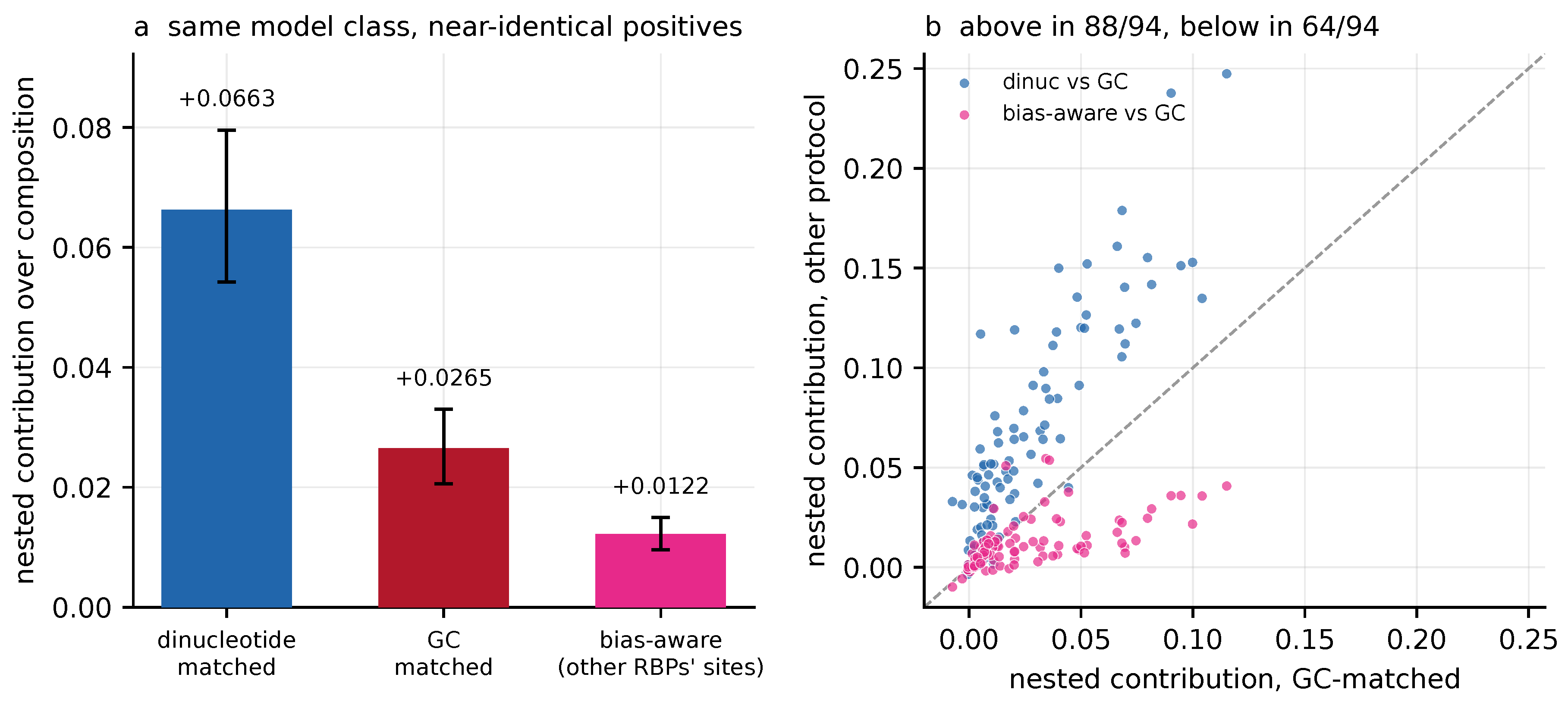
Figure 2.
Fold span in nested contribution across the three protocols under eight monotone rescalings of the same 282 protocol-dataset cells. Seven of the eight are shown; normalising by the excess over chance is omitted because its span of 18.2 is off scale. Points are the span and bars are 95% percentile intervals from a bootstrap over the 79 proteins (4000 draws); the dashed line marks protocol independence. Somers’ D is an affine map of AUROC and returns the raw value by construction, serving as an internal control. The smallest span, 2.00 (1.67–2.46), is obtained by dividing by the headroom of the baseline.
Figure 2.
Fold span in nested contribution across the three protocols under eight monotone rescalings of the same 282 protocol-dataset cells. Seven of the eight are shown; normalising by the excess over chance is omitted because its span of 18.2 is off scale. Points are the span and bars are 95% percentile intervals from a bootstrap over the 79 proteins (4000 draws); the dashed line marks protocol independence. Somers’ D is an affine map of AUROC and returns the raw value by construction, serving as an internal control. The smallest span, 2.00 (1.67–2.46), is obtained by dividing by the headroom of the baseline.
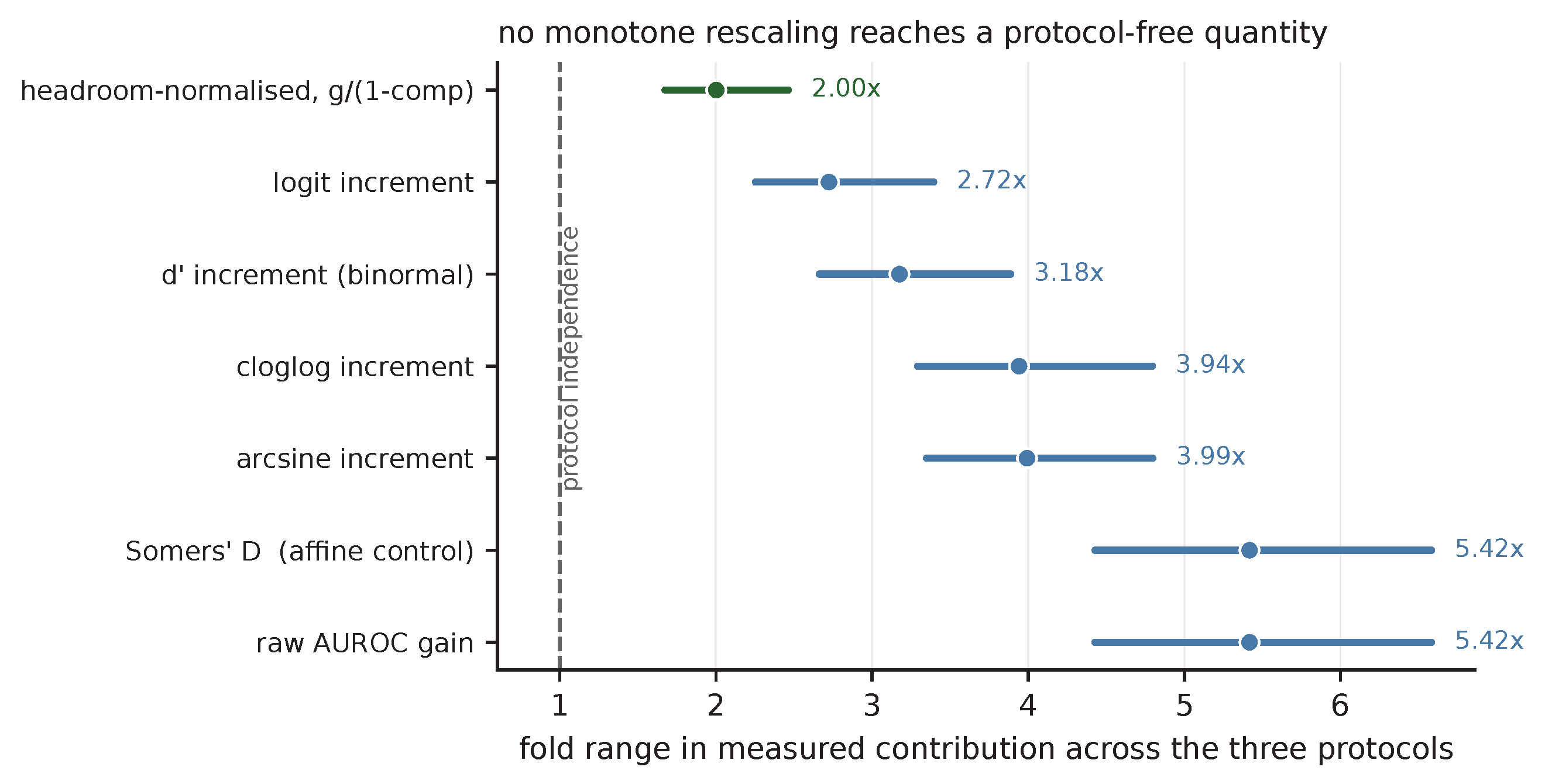
Figure 3.
(a) All 282 protocol-dataset cells: nested contribution against the composition-only AUROC left by the protocol, by protocol (pooled Spearman , ). (b) Datasets partitioned by whether the bias-aware protocol raised or lowered the composition baseline relative to GC matching ( and 27); points are stratum means and bars are 95% percentile intervals from a bootstrap over datasets (4000 draws). The contribution deficit is abolished where the baseline falls.
Figure 3.
(a) All 282 protocol-dataset cells: nested contribution against the composition-only AUROC left by the protocol, by protocol (pooled Spearman , ). (b) Datasets partitioned by whether the bias-aware protocol raised or lowered the composition baseline relative to GC matching ( and 27); points are stratum means and bars are 95% percentile intervals from a bootstrap over datasets (4000 draws). The contribution deficit is abolished where the baseline falls.
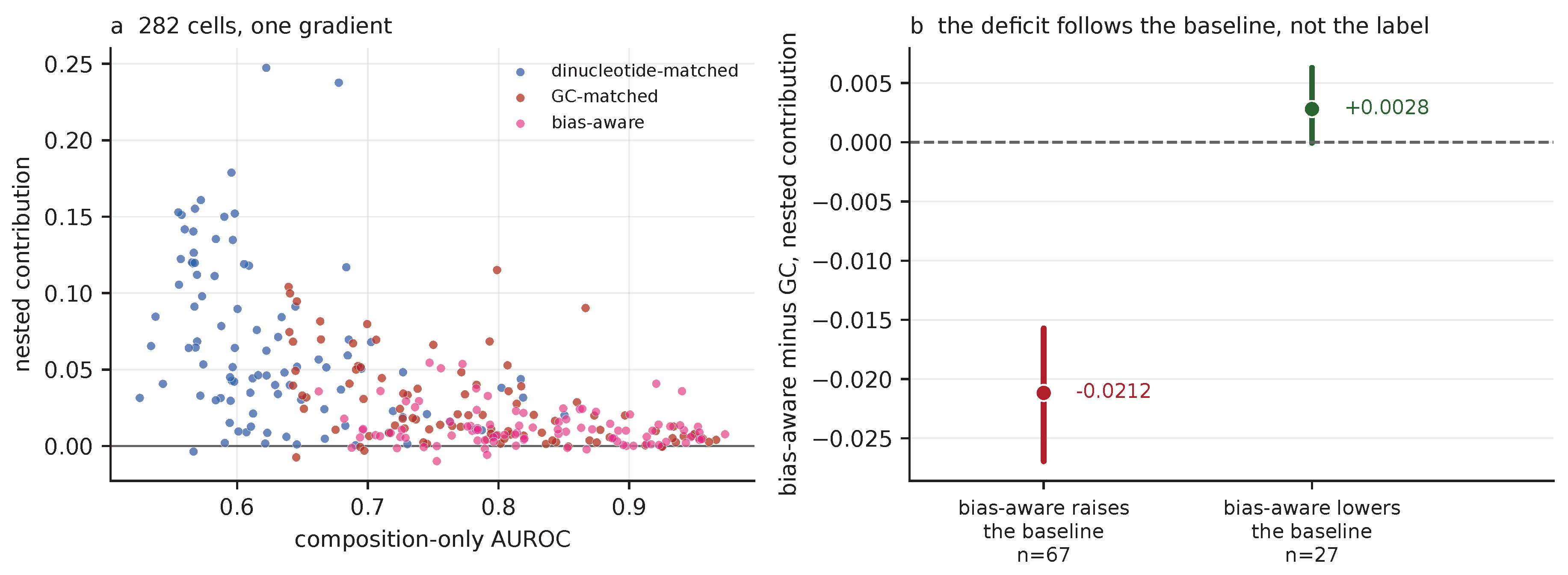
Figure 4.
Three model classes on identical rows and folds within each arm, datasets: a 4-mer logistic regression, a 7089-parameter convolutional network and a fully fine-tuned 19.78 M-parameter SpliceBERT. (a) Nested contribution in each composition-matched arm, per model; bars are 95% protein-clustered percentile intervals, as in panel (b). (b) The two-arm contrast per model, with 95% percentile intervals from a bootstrap over the 79 proteins taking all datasets of each sampled protein (4000 draws). The hatched band spans the protocol effect obtained by transplanting a discriminability increment in either direction, to for the 4-mer, to for the convolutional network and to for SpliceBERT: every member keeps the sign, so the contrast is not an artefact of AUROC compression, but its width is why I report the raw contrast and decline the decomposition in the text. (c) The contrast per dataset, SpliceBERT against the 4-mer; it is larger for SpliceBERT in all 94.
Figure 4.
Three model classes on identical rows and folds within each arm, datasets: a 4-mer logistic regression, a 7089-parameter convolutional network and a fully fine-tuned 19.78 M-parameter SpliceBERT. (a) Nested contribution in each composition-matched arm, per model; bars are 95% protein-clustered percentile intervals, as in panel (b). (b) The two-arm contrast per model, with 95% percentile intervals from a bootstrap over the 79 proteins taking all datasets of each sampled protein (4000 draws). The hatched band spans the protocol effect obtained by transplanting a discriminability increment in either direction, to for the 4-mer, to for the convolutional network and to for SpliceBERT: every member keeps the sign, so the contrast is not an artefact of AUROC compression, but its width is why I report the raw contrast and decline the decomposition in the text. (c) The contrast per dataset, SpliceBERT against the 4-mer; it is larger for SpliceBERT in all 94.
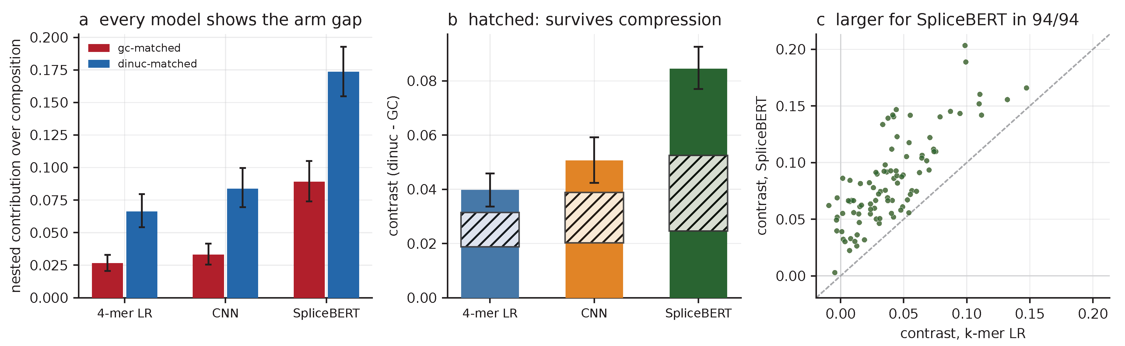
Figure 5.
Nested contribution against the order of the composition baseline, datasets, in each negative-set protocol: (a) dinucleotide-matched, (b) GC-matched, (c) bias-aware. Top row, contribution for each model class, with 95% protein-clustered percentile intervals as bands; the step from order three to order four is dashed because it crosses out of the range where the baseline is a baseline. Bottom row, the composition baseline’s own out-of-fold AUROC, which is the diagnostic: the shaded region marks order four, where a 337-column block overfits and its own AUROC falls on 34, 52 and 64 of the 94 datasets. The 4-mer’s contribution rises there while the two neural models’ continue to fall, because the order-four block spans the 4-mer’s feature space and its pre-fit score repairs a fit the baseline cannot achieve alone. Panel means can still rise where the per-dataset AUROC falls on a minority of datasets, which is why the counts are given.
Figure 5.
Nested contribution against the order of the composition baseline, datasets, in each negative-set protocol: (a) dinucleotide-matched, (b) GC-matched, (c) bias-aware. Top row, contribution for each model class, with 95% protein-clustered percentile intervals as bands; the step from order three to order four is dashed because it crosses out of the range where the baseline is a baseline. Bottom row, the composition baseline’s own out-of-fold AUROC, which is the diagnostic: the shaded region marks order four, where a 337-column block overfits and its own AUROC falls on 34, 52 and 64 of the 94 datasets. The 4-mer’s contribution rises there while the two neural models’ continue to fall, because the order-four block spans the 4-mer’s feature space and its pre-fit score repairs a fit the baseline cannot achieve alone. Panel means can still rise where the per-dataset AUROC falls on a minority of datasets, which is why the counts are given.
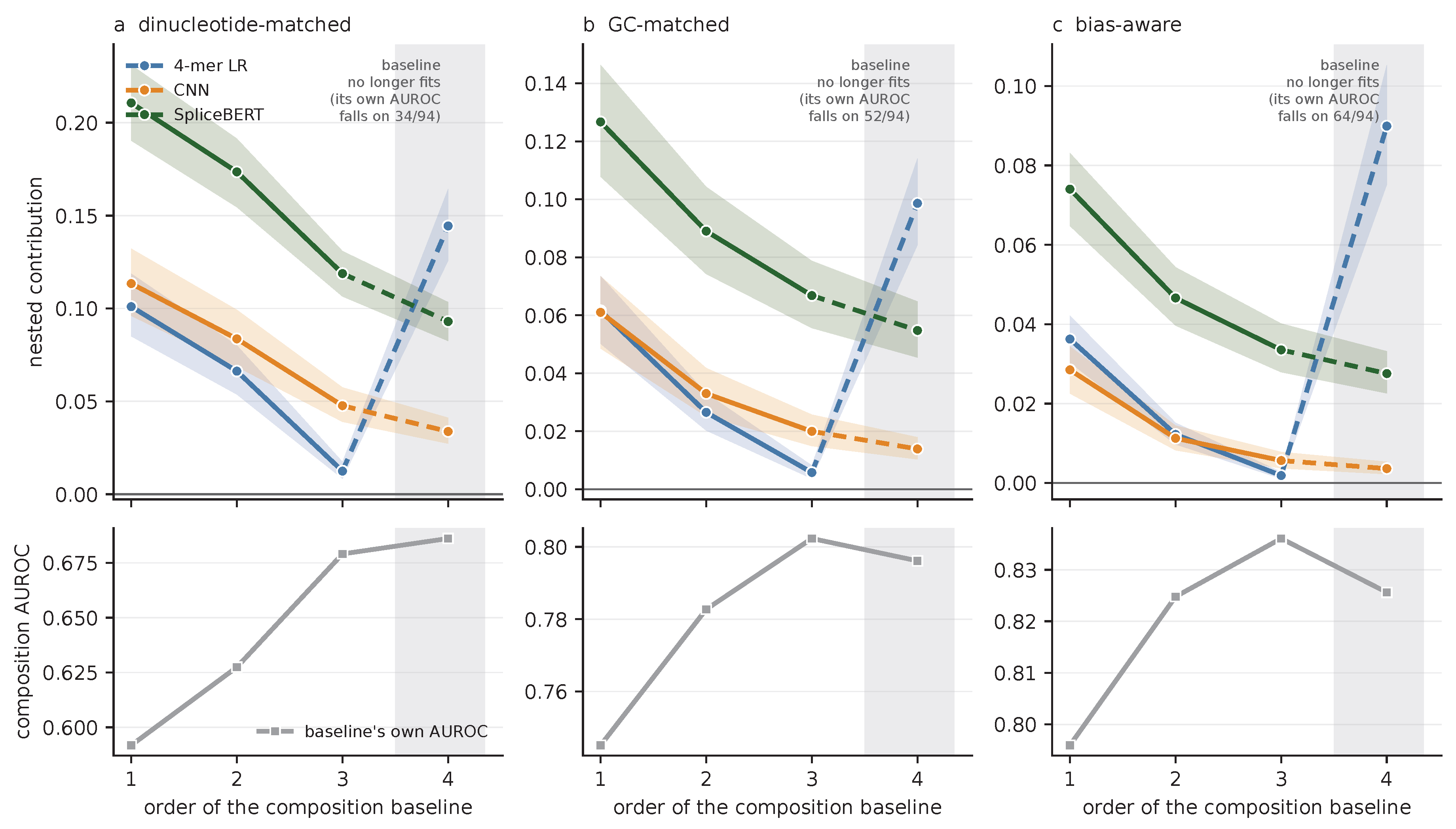
Figure 6.
Replication using the released negative sets, peak calling and fold assignments of Horlacher et al. [4], over the 45 datasets shared with the study panel; only the measurement was performed in this study. (a) Nested contribution under their negative-2 against their negative-1, paired by dataset; 36 of 45 lie below the diagonal. (b) Within-arm Spearman correlation between the composition baseline and the contribution, for the composition-matched arms of both benchmarks and the other-RBPs’-sites arms of both, with percentile intervals over resampled proteins. The three composition-matched arms exclude zero and the two other-RBPs’-sites arms do not, independently in each benchmark. The grouping this invites is not stable to which term is placed on the horizontal axis and is not endorsed in Section 3.4; what the panel supports is the narrower statement about where the gradient is detectable.
Figure 6.
Replication using the released negative sets, peak calling and fold assignments of Horlacher et al. [4], over the 45 datasets shared with the study panel; only the measurement was performed in this study. (a) Nested contribution under their negative-2 against their negative-1, paired by dataset; 36 of 45 lie below the diagonal. (b) Within-arm Spearman correlation between the composition baseline and the contribution, for the composition-matched arms of both benchmarks and the other-RBPs’-sites arms of both, with percentile intervals over resampled proteins. The three composition-matched arms exclude zero and the two other-RBPs’-sites arms do not, independently in each benchmark. The grouping this invites is not stable to which term is placed on the horizontal axis and is not endorsed in Section 3.4; what the panel supports is the narrower statement about where the gradient is detectable.
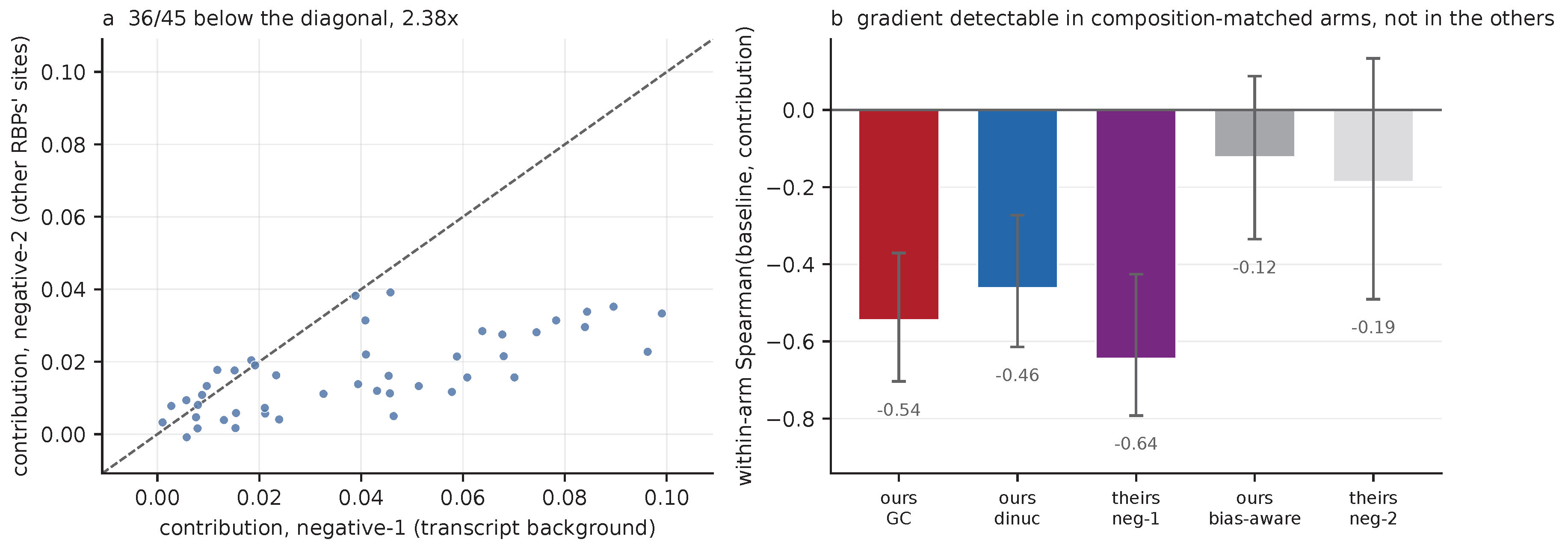
Figure 7.
(a) Cross-protocol rank agreement between nested contributions before and after division by the headroom of the baseline, for each of the three protocol pairs in the study data. Agreement improves in 3 of 3 pairs; only the GC-versus-dinucleotide improvement has a protein-clustered interval excluding zero. (b) The same test on the externally constructed benchmark of Figure 6, : rank agreement falls and disagreement rises under normalisation, the two criteria fixed before the external data were scored as falsifying. The change in rank agreement is ( to ), a failure to replicate rather than a refutation.
Figure 7.
(a) Cross-protocol rank agreement between nested contributions before and after division by the headroom of the baseline, for each of the three protocol pairs in the study data. Agreement improves in 3 of 3 pairs; only the GC-versus-dinucleotide improvement has a protein-clustered interval excluding zero. (b) The same test on the externally constructed benchmark of Figure 6, : rank agreement falls and disagreement rises under normalisation, the two criteria fixed before the external data were scored as falsifying. The change in rank agreement is ( to ), a failure to replicate rather than a refutation.
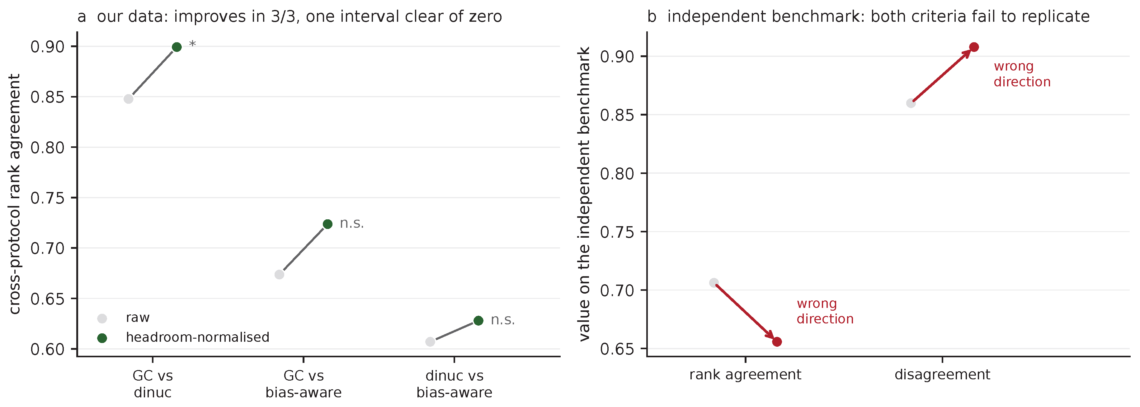

Table 1.
Achieved match quality between each positive and its assigned negative, all pairs. Columns three to six describe the absolute GC difference between the pair; is over the sixteen dinucleotide frequencies, on a 0 to 2 scale. The 0.05 column is a common yardstick and is the GC matcher’s nominal tolerance; the dinucleotide matcher has no GC tolerance to hold.
Table 1.
Achieved match quality between each positive and its assigned negative, all pairs. Columns three to six describe the absolute GC difference between the pair; is over the sixteen dinucleotide frequencies, on a 0 to 2 scale. The 0.05 column is a common yardstick and is the GC matcher’s nominal tolerance; the dinucleotide matcher has no GC tolerance to hold.
| arm | pairs | med. GC| | p90 | p99 | max | GC | med. |
|---|---|---|---|---|---|---|---|
| GC-matched | 456,734 | 0.0297 | 0.0495 | 0.1089 | 0.1486 | 94.8% | 0.500 |
| dinucleotide-matched | 457,998 | 0.0198 | 0.0693 | 0.1485 | 0.4159 | 85.0% | 0.220 |
| bias-aware | 456,734 | 0.1387 | 0.3169 | 0.4555 | 0.6733 | 20.4% | 0.700 |
Table 2.
Composition-only AUROC, the 4-mer’s own AUROC, the AUROC of the two together, and the nested contribution, under three negative-set protocols. The nested contribution is the composition-plus-4-mer column minus the composition-alone column by construction. The 4-mer’s own AUROC is what a study would report as its headline. Model class, folds and estimator are identical across arms and the model is refitted under each; positives are identical in 10 of 94 datasets and share a median Jaccard of 0.997, as the Limitations set out. datasets.
Table 2.
Composition-only AUROC, the 4-mer’s own AUROC, the AUROC of the two together, and the nested contribution, under three negative-set protocols. The nested contribution is the composition-plus-4-mer column minus the composition-alone column by construction. The 4-mer’s own AUROC is what a study would report as its headline. Model class, folds and estimator are identical across arms and the model is refitted under each; positives are identical in 10 of 94 datasets and share a median Jaccard of 0.997, as the Limitations set out. datasets.
| protocol | composition | 4-mer alone | composition + 4-mer | contribution |
|---|---|---|---|---|
| dinucleotide-matched | 0.6274 | 0.6879 | 0.6937 | |
| GC-matched | 0.7827 | 0.7981 | 0.8092 | |
| bias-aware | 0.8248 | 0.8169 | 0.8370 |
Table 3.
What the region label alone achieves in each arm, and the bias-aware arm rebuilt with region matched. Region is matched by construction in both composition-matched arms and free in the bias-aware arm. The rebuilt arm is a diagnostic, not a fourth protocol; the reweighted row is a second estimate from a different construction, which discards 30% of the rows. datasets.
Table 3.
What the region label alone achieves in each arm, and the bias-aware arm rebuilt with region matched. Region is matched by construction in both composition-matched arms and free in the bias-aware arm. The rebuilt arm is a diagnostic, not a fourth protocol; the reweighted row is a second estimate from a different construction, which discards 30% of the rows. datasets.
| arm | pairs kept | region AUROC | region TV | composition | contribution |
|---|---|---|---|---|---|
| dinucleotide-matched | 100% | 0.5000 | 0.0000 | 0.6274 | |
| GC-matched | 100% | 0.5000 | 0.0000 | 0.7827 | |
| bias-aware | 100% | 0.7484 | 0.4192 | 0.8248 | |
| bias-aware, region-matched | 100% | 0.5000 | 0.0000 | 0.8052 | |
| the same, by reweighting | 70% | 0.5026 | 0.0043 | 0.8017 |
Table 4.
Fold span across the three protocols for , where g is the nested contribution and c the composition-only AUROC, under three ways of aggregating the same 282 cells. Only the mean of per-dataset ratios, the aggregation used throughout this paper, approaches unity; it is also the one a denominator of 0.027 can dominate. The final column is the minimum over p on and the exponent attaining it.
Table 4.
Fold span across the three protocols for , where g is the nested contribution and c the composition-only AUROC, under three ways of aggregating the same 282 cells. Only the mean of per-dataset ratios, the aggregation used throughout this paper, approaches unity; it is also the one a denominator of 0.027 can dominate. The final column is the minimum over p on and the exponent attaining it.
| p | 0 | 0.5 | 1.0 | 1.25 | 1.544 | 1.75 | 2.0 | min | at p |
|---|---|---|---|---|---|---|---|---|---|
| mean of ratios | 5.42 | 3.43 | 2.00 | 1.48 | 1.004 | 1.34 | 1.95 | 1.004 | 1.54 |
| median of ratios | 5.09 | 3.92 | 2.61 | 2.34 | 1.70 | 1.37 | 1.29 | 1.238 | 2.17 |
| ratio of means | 5.42 | 3.62 | 2.55 | 2.17 | 1.82 | 1.61 | 1.44 | 1.278 | 2.64 |
Table 5.
Attribution of variance in the nested contribution, and the within-arm relation between baseline and contribution, by model class ().
Table 5.
Attribution of variance in the nested contribution, and the within-arm relation between baseline and contribution, by model class ().
| incremental | within-arm Spearman | ||||
|---|---|---|---|---|---|
| model | protocol ∣ base | base ∣ protocol | dinuc | GC | bias-aware |
| 4-mer | 1.00% | 11.05% | |||
| CNN | 4.60% | 3.47% | |||
| SpliceBERT | 1.12% | 25.62% | |||
Table 6.
Negative-set construction and baseline reporting in a targeted, non-systematic sample of seven methods and benchmarks. Coordinate: negatives are genomic intervals relocated within genes or transcripts that carry a positive. Other RBPs: negatives are binding sites of different proteins. The composition-baseline column records whether a composition-only AUROC is reported alongside the method’s headline AUROC.
Table 6.
Negative-set construction and baseline reporting in a targeted, non-systematic sample of seven methods and benchmarks. Coordinate: negatives are genomic intervals relocated within genes or transcripts that carry a positive. Other RBPs: negatives are binding sites of different proteins. The composition-baseline column records whether a composition-only AUROC is reported alongside the method’s headline AUROC.
| source | year | negatives | composition baseline |
|---|---|---|---|
| GraphProt [19] | 2014 | coordinate | no |
| RBP-24 dataset [26] | 2018 | coordinate | no |
| pysster [27] | 2018 | other RBPs | no |
| DeepCLIP [28] | 2020 | coordinate | no |
| RNAProt [29] | 2021 | coordinate | no |
| Horlacher et al. benchmark [4] | 2023 | other RBPs | no |
| RBPsuite 2.0 [30] | 2025 | coordinate | no |
Table 7.
Four negative-set constructions, the 4-mer logistic regression, datasets, identical folds. The shuffled arm uses the GC arm’s positives exactly; the GC and dinucleotide arms’ retained positives are near-identical rather than identical, because each arm keeps only the positives its own matching could pair (median Jaccard , minimum , identical in 10 of 94; results/tables/positive_set_overlap.csv). The three matched arms are Table 8’s first row; the shuffled arm generates each negative from its own positive.
Table 7.
Four negative-set constructions, the 4-mer logistic regression, datasets, identical folds. The shuffled arm uses the GC arm’s positives exactly; the GC and dinucleotide arms’ retained positives are near-identical rather than identical, because each arm keeps only the positives its own matching could pair (median Jaccard , minimum , identical in 10 of 94; results/tables/positive_set_overlap.csv). The three matched arms are Table 8’s first row; the shuffled arm generates each negative from its own positive.
| construction | composition alone | contribution | standalone AUROC |
|---|---|---|---|
| dinucleotide-shuffled | 0.5000 | 0.7528 | |
| dinucleotide-matched | 0.6274 | ||
| GC-matched | 0.7827 | ||
| bias-aware | 0.8248 |
Table 8.
Nested contribution under three negative-set protocols for three model classes, datasets. Within each arm the three model classes are scored on identical rows and folds, which is what makes the across-model comparison exact; rows differ between arms by construction. Spans are ratios of panel means with protein-clustered percentile intervals.
Table 8.
Nested contribution under three negative-set protocols for three model classes, datasets. Within each arm the three model classes are scored on identical rows and folds, which is what makes the across-model comparison exact; rows differ between arms by construction. Spans are ratios of panel means with protein-clustered percentile intervals.
| model | dinucleotide | GC | bias-aware | span |
|---|---|---|---|---|
| 4-mer | 5.42 (4.43–6.58) | |||
| CNN | 7.42 (6.07–9.31) | |||
| SpliceBERT | 3.72 (3.23–4.30) | |||
| composition alone | 0.6274 | 0.7827 | 0.8248 |
Table 9.
Model-alone out-of-fold AUROC, three model classes under three protocols, datasets, with the composition-only baseline for reference. Each model’s figure is pooled over every row that model covers, which is what a benchmark reports and which differs between models by 0.06% of rows. The rightmost column is the protocol each model finds easiest.
Table 9.
Model-alone out-of-fold AUROC, three model classes under three protocols, datasets, with the composition-only baseline for reference. Each model’s figure is pooled over every row that model covers, which is what a benchmark reports and which differs between models by 0.06% of rows. The rightmost column is the protocol each model finds easiest.
| dinucleotide | GC | bias-aware | easiest | |
|---|---|---|---|---|
| composition alone | 0.6274 | 0.7827 | 0.8248 | bias-aware |
| 4-mer | 0.6879 | 0.7981 | 0.8169 | bias-aware |
| CNN | 0.7076 | 0.8084 | 0.8162 | bias-aware |
| SpliceBERT | 0.8099 | 0.8771 | 0.8732 | GC |
Table 10.
The same nested comparison on five estimands, panel means over datasets. The ordering dinucleotide > GC > bias-aware holds in all 15 estimand-by-model cells. Spans are the largest arm mean over the smallest. Deviance and McFadden are computed on the scale the model is fitted on and are unbounded above, so they carry no ceiling.
Table 10.
The same nested comparison on five estimands, panel means over datasets. The ordering dinucleotide > GC > bias-aware holds in all 15 estimand-by-model cells. Spans are the largest arm mean over the smallest. Deviance and McFadden are computed on the scale the model is fitted on and are unbounded above, so they carry no ceiling.
| estimand | model | dinucleotide | GC | bias-aware | span |
|---|---|---|---|---|---|
| AUROC increment | 4-mer | 0.0663 | 0.0265 | 0.0122 | 5.42 |
| CNN | 0.0837 | 0.0330 | 0.0113 | 7.42 | |
| SpliceBERT | 0.1735 | 0.0890 | 0.0466 | 3.72 | |
| deviance | 4-mer | 967 | 761 | 462 | 2.09 |
| CNN | 1659 | 1185 | 536 | 3.09 | |
| SpliceBERT | 3524 | 2944 | 1656 | 2.13 | |
| McFadden increment | 4-mer | 0.0520 | 0.0380 | 0.0244 | 2.13 |
| CNN | 0.0784 | 0.0523 | 0.0240 | 3.27 | |
| SpliceBERT | 0.1905 | 0.1543 | 0.0925 | 2.06 | |
| average precision increment | 4-mer | 0.0551 | 0.0276 | 0.0149 | 3.70 |
| CNN | 0.0755 | 0.0355 | 0.0131 | 5.78 | |
| SpliceBERT | 0.1580 | 0.0917 | 0.0497 | 3.18 | |
| IDI | 4-mer | 0.0669 | 0.0448 | 0.0279 | 2.40 |
| CNN | 0.1038 | 0.0666 | 0.0320 | 3.25 | |
| SpliceBERT | 0.2419 | 0.1851 | 0.1129 | 2.14 |
Table 11.
Nested contribution over an order-three composition baseline, datasets, identical rows, folds and model scores to Table 8. Surviving is the order-three contribution as a fraction of the order-two one, as a ratio of panel means; the range is over the three arms. Spans are ratios of panel means with protein-clustered percentile intervals.
Table 11.
Nested contribution over an order-three composition baseline, datasets, identical rows, folds and model scores to Table 8. Surviving is the order-three contribution as a fraction of the order-two one, as a ratio of panel means; the range is over the three arms. Spans are ratios of panel means with protein-clustered percentile intervals.
| model | dinucleotide | GC | bias-aware | span | surviving |
|---|---|---|---|---|---|
| 4-mer | 6.60 (4.71–10.05) | 0.154–0.217 | |||
| CNN | 8.43 (6.49–11.64) | 0.502–0.605 | |||
| SpliceBERT | 3.54 (3.05–4.11) | 0.685–0.750 | |||
| composition alone | 0.6791 | 0.8023 | 0.8361 | ||
| rise from order two |
Table 12.
Nested contribution against the order of the composition baseline, datasets. Baseline width counts columns after one is dropped per frequency family and entropy is appended. Order four is not a baseline: see the text.
Table 12.
Nested contribution against the order of the composition baseline, datasets. Baseline width counts columns after one is dropped per frequency family and entropy is appended. Order four is not a baseline: see the text.
| order 1 | order 2 | order 3 | order 4 | ||
|---|---|---|---|---|---|
| baseline width | 4 | 19 | 82 | 337 | |
| dinucleotide | composition alone | 0.5918 | 0.6274 | 0.6791 | 0.6861 |
| 4-mer | |||||
| CNN | |||||
| SpliceBERT | |||||
| GC | composition alone | 0.7451 | 0.7827 | 0.8023 | 0.7961 |
| 4-mer | |||||
| CNN | |||||
| SpliceBERT | |||||
| bias-aware | composition alone | 0.7959 | 0.8248 | 0.8361 | 0.8256 |
| 4-mer | |||||
| CNN | |||||
| SpliceBERT |
Table 13.
Nested contribution of a 4-mer when the training and evaluation protocols are varied separately, datasets. Rows are the protocol whose windows the model was fitted on; columns are the protocol whose windows it was scored on. The diagonal is the published within-arm result. Varying the row moves the contribution by 0.0141, varying the column by 0.0438.
Table 13.
Nested contribution of a 4-mer when the training and evaluation protocols are varied separately, datasets. Rows are the protocol whose windows the model was fitted on; columns are the protocol whose windows it was scored on. The diagonal is the published within-arm result. Varying the row moves the contribution by 0.0141, varying the column by 0.0438.
| evaluated on | |||
|---|---|---|---|
| trained on | GC | dinucleotide | bias-aware |
| GC | |||
| dinucleotide | |||
| bias-aware | |||
Table 14.
The external analysis under both estimators and both fold partitions. All four cells meet the numerical thresholds fixed in the original protocol, before the 135-dataset complement was scored. The directional estimand and the two repairs were specified afterwards, in a dated amendment, and before those two cells were computed. The first row is the published analysis recomputed, and reproduces it to , which is what makes the other three readable. Intervals are 95% protein-clustered percentile bootstraps over 4000 draws, seed fixed in the amendment.
Table 14.
The external analysis under both estimators and both fold partitions. All four cells meet the numerical thresholds fixed in the original protocol, before the 135-dataset complement was scored. The directional estimand and the two repairs were specified afterwards, in a dated amendment, and before those two cells were computed. The first row is the published analysis recomputed, and reproduces it to , which is what makes the other three readable. Intervals are 95% protein-clustered percentile bootstraps over 4000 draws, seed fixed in the amendment.
| folds | estimator | R (95% CI) | verdict |
|---|---|---|---|
| supplied | two-stage | 1.69 (1.41–2.03) | supports |
| supplied | cross-fitted | 1.66 (1.40–1.98) | supports |
| chromosome-blocked | two-stage | 1.73 (1.43–2.10) | supports |
| chromosome-blocked | cross-fitted | 1.67 (1.40–2.00) | supports |
Table 15.
The nested estimator applied to a model whose information the baseline already contains, so the true contribution is zero. datasets, order-two baseline, the same rows, folds and estimator as every other result here. Intervals are protein-clustered.
Table 15.
The nested estimator applied to a model whose information the baseline already contains, so the true contribution is zero. datasets, order-two baseline, the same rows, folds and estimator as every other result here. Intervals are protein-clustered.
| arm | measured floor | 95% interval | reported contribution |
|---|---|---|---|
| dinucleotide | to | ||
| GC | to | ||
| bias-aware | to |
Table 16.
The outer-fold information route, measured by closing it. Contribution as published and fully cross-fitted, datasets, protein-clustered intervals. The 2-mer’s true contribution is zero by construction; the 4-mer’s is not known. Positive channel means the published value was inflated.
Table 16.
The outer-fold information route, measured by closing it. Contribution as published and fully cross-fitted, datasets, protein-clustered intervals. The 2-mer’s true contribution is zero by construction; the 4-mer’s is not known. Positive channel means the published value was inflated.
| model | arm | as published | cross-fitted | channel |
|---|---|---|---|---|
| 4-mer | dinucleotide | |||
| GC | ||||
| bias-aware | ||||
| 2-mer | dinucleotide | |||
| GC | ||||
| bias-aware |
Table 17.
The same decomposition applied to the released negative sets of Horlacher et al. [4], datasets. Their release does not supply a model-only AUROC, so difficulty in this table is read from the composition baseline; the 4-mer’s own AUROC on their negative sets is computed by this study and reported in the text below.
Table 17.
The same decomposition applied to the released negative sets of Horlacher et al. [4], datasets. Their release does not supply a model-only AUROC, so difficulty in this table is read from the composition baseline; the 4-mer’s own AUROC on their negative sets is computed by this study and reported in the text below.
| negative set | composition | composition + 4-mer | contribution |
|---|---|---|---|
| negative-1 (transcript background) | 0.8211 | 0.8606 | |
| negative-2 (other RBPs’ sites) | 0.7560 | 0.7726 |
Disclaimer/Publisher’s Note: The statements, opinions and data contained in all publications are solely those of the individual author(s) and contributor(s) and not of MDPI and/or the editor(s). MDPI and/or the editor(s) disclaim responsibility for any injury to people or property resulting from any ideas, methods, instructions or products referred to in the content. |
© 2026 by the author. Licensee MDPI, Basel, Switzerland. This article is an open access article distributed under the terms and conditions of the Creative Commons Attribution (CC BY) license.
Copyright: This open access article is published under a Creative Commons CC BY 4.0 license, which permit the free download, distribution, and reuse, provided that the author and preprint are cited in any reuse.