

Submitted:
09 September 2026
Posted:
10 September 2026
You are already at the latest version
Abstract
The objective of this study was to evaluate the effect of the carbon source (CS), the nitrogen source (NS), the percentage of pumpkin (PJ) in the juice, and heat treatment (TT) on the growth of Streptococcus thermophilus and Lactobacillus delbrueckii subsp. bulgaricus, in order to develop an inoculum adapted to a plant-based matrix. The experimental process included a screening design, maximum rise trajectory, and response surface optimization, supplemented by principal component analysis (PCA). Cell viability was determined by microbiological count (CFU/mL) and expressed as the logarithmic increase in cell viability (LIV). The screening identified CS, NS, and PJ as significant factors (p = 0.003). The optimization predicted a maximum LVI of 8.17 with 8.0% CS, 7.26% NS, and 7.28% PJ. The model had an R2 of 89.22% and a standard error of less than 10%. PCA explained 79.81% of the variability through two components (PC1 = 61.02% and PC2 = 18.80%), associating PC1 with conductivity, salinity, and suspended solids, and PC2 with pH, total solids, and titratable acidity, demonstrating the relationship between microbial growth and physicochemical changes during fermentation.
Keywords:
lactic acid bacteria
; fermentation
; inoculum
; pumpkin juice
; optimization
1. Introduction
Pumpkin (Cucurbita moschata) is a species of the Cucurbitaceae family that originated in tropical and subtropical regions [1]. Pumpkin pulp is characterized by a broad nutritional profile, with protein contents ranging from 0.52 to 13.42% [2], fat contents of up to 16.7% [3], carbohydrate contents ranging from 7.52 to 40.32% [4], fiber contents ranging from 1.6 to 13.35% [5] , and minerals such as magnesium, zinc, calcium, sodium, potassium, and iron [6,7,8]. This nutritional profile supports the use of pumpkin pulp as a promising plant matrix for biotechnological processes focused on the production of ingredients, fermented foods, and products with functional potential.
Lactic acid bacteria (LAB) have been studied in various plant matrices for kinetic modeling, fermentation processes, storage studies, and the formulation of probiotic beverages [9,10,11]. Research on pumpkin juice has examined different LAB strains by determining microbial viability, physicochemical changes, functional properties, and the probiotic potential of the resulting products [12,13,14]. These studies demonstrate the potential of plant matrices as substrates for lactic acid fermentation. However, they also indicate that microbial responses depend on matrix composition, the strain used, and the activation and incubation conditions.
The development of LAB inoculum in plant matrices represents a technologically relevant strategy as it facilitates the evaluation of cell viability in nonconventional substrates and promotes the physiological adaptation of microorganisms to the medium in which they will subsequently grow. Such adaptation may improve the utilization of nutrients present in the matrix, increase the stability of fermentation processes, and improve process reproducibility. Moreover, using plant matrices as media for microbial activation or propagation may reduce dependence on conventional microbiological media, which are generally more expensive, without restricting the synthesis of functional metabolites relevant to food applications.
Plant matrices, however, are complex and variable systems whose composition may not fully satisfy the nutritional requirements of LAB. Supplementation with carbon and nitrogen sources is therefore necessary to support the viability, stability, and metabolic activity of the inoculum [15,16,17], given that microbial growth is governed by both substrate availability and incubation conditions [16].
The carbon source provides the primary energy supply for cellular maintenance and microbial growth. Together with the nitrogen source, it may also influence the synthesis of functional metabolites such as exopolysaccharides (EPS), which are of interest because of their potential effects on the rheological, technological, and functional properties of fermented systems. The concentration and origin of these nutritional sources may modify the molecular weight of EPS, the concentration of the metabolite produced, and its production kinetics [15,18,19,20]. Fructose, lactose, glucose, and sucrose are among the most extensively studied carbon sources [20], Depending on the microbial species and process conditions, these sugars may be metabolized through homofermentative or heterofermentative pathways [19].
The nitrogen source supplies amino acids, peptides, nitrogenous bases, vitamins, and other growth factors required for LAB metabolism. Previous studies have examined substrates such as casein hydrolysate, peptone, meat extract, soybean flour, and yeast extract [15,16,17]. Yeast extract has been identified as one of the most efficient nitrogen sources, due to its high content of nitrogenous compounds, purine and pyrimidine bases, and vitamins [20,21]. However, the cost of yeast extract may limit process scalability and reproducibility. Consequently, the exploration of lower-cost and widely available alternatives capable of providing the nutrients required for inoculum development remains necessary [22,23].
In this context, optimizing inoculum activation conditions is essential to ensure the development of a viable LAB population in a plant-based matrix such as pumpkin. However, interactions among medium components can make microbial responses difficult to interpret when factors are evaluated individually. Therefore, sequential statistical approaches, such as response surface methodology, are useful to identify the most influential variables, guide the exploration of improved conditions, and determine an optimized formulation while reducing the number of experimental runs required.
This study aimed to develop and optimize a LAB inoculum in pumpkin juice through a sequential response surface methodology. The experimental design consisted of three stages: (i) a screening design to identify the formulation and process factors with the greatest influence on inoculum viability; (ii) construction of the path of steepest ascent based on the selected first-order model; and (iii) application of a response surface design to examine system curvature, optimize the formulation, and experimentally validate the predicted condition.
2. Materials and Methods
2.1. Materials
Pumpkin (Cucurbita moschata) was purchased from a supermarket in Cali, Valle del Cauca, Colombia. The raw material was selected based on the absence of mechanical damage, visible microbial deterioration, pests, and other contaminants. The pumpkin was then transported to the Bioprocess Laboratory at Universidad del Valle (Cali, Valle del Cauca) and disinfected by immersion in a 2% sodium hypochlorite solution for 15 min.
A commercial freeze-dried starter culture for yogurt production (Frutaroma–Delix), containing Streptococcus thermophilus and Lactobacillus delbrueckii subsp. bulgaricus, was used. Commercial sucrose and powdered milk (El Rodeo) served as the carbon source (CS) and nitrogen source (NS), respectively.
2.2. Technological Processes
2.2.1. Juice Preparation
The disinfected pumpkin was peeled and cut into cubes. Pumpkin juice was prepared using a blender (Black+Decker, Beijing, China) with the quantities of pumpkin and water specified for each experimental treatment, as described in Section Screening Design. Under sterile conditions, 180 mL portions of juice were transferred into sterile airtight containers. The juice was thermally treated in an autoclave (Trident, Taipei, Taiwan) at 121 °C for 15 min. After thermal treatment, the samples were cooled at room temperature to approximately 18 °C.
2.3. Fermentation
2.3.1. Stock Culture Suspension
The commercial starter culture was prepared by suspending 1.2 g of the freeze-dried microbial mixture in 100 mL of peptone water. The suspension was mixed until complete dispersion and incubated at 42 °C for 15 min in an incubator (Binder, Berlín, Alemania).
2.3.2. Inoculation
The quantities of CS and NS required for each treatment were weighed in previously disinfected containers. Each supplement was added to the corresponding juice treatment and mixed until a homogeneous system was obtained.
Following incubation of the stock culture suspension, each treatment was inoculated with 1 mL of the suspension to obtain a comparable initial microbial concentration across treatments. Microbial initial counts were determined immediately after inoculation. The containers were then sealed and incubated for 48 h, after which the final microbial population was quantified.
2.4. Analytical Methods
2.4.1. Microbial Viability
Microbial populations were quantified through serial dilution by transferring 1 mL of each sample into 9 mL of peptone water (Scharlau, Barcelona, Spain). Microbial counts were determined using the microdrop plating method [24]. Dilutions from 10−1 to 10−6 were plated on de Man, Rogosa, and Sharpe agar (MRS; Scharlau, Barcelona, Spain) and incubated at 42 °C according to [25]. Results were expressed as colony-forming units per milliliter (CFU/mL).
2.4.2. pH
The pH of the inoculated juice was measured at the beginning and end of each fermentation process according to AOAC Method 981.12 [26] using a calibrated pH meter (Thermo Scientific, EE. UU).
2.4.3. Titratable Acidity
Titratable acidity was determined after diluting the juice with distilled water at a ratio of 1:10 (v/v). The diluted sample was titrated with 0.0997 N sodium hydroxide using phenolphthalein as the endpoint indicator. Results were expressed as lactic acid equivalents according to AOAC Method 942.15 [26].
2.4.4. Soluble Solids
Soluble solids content (°Brix) was measured in the inoculated juices at the beginning and end of fermentation using a portable digital refractometer (Atago, Tokyo, Japan), according to AOAC Method 932.12 [26].
2.4.5. Suspended Solids, Conductivity and Salinity
Total dissolved solids (mg/L), electrical conductivity (µS/cm), and salinity (%) were measured in the inoculated juices at the beginning and end of fermentation using a previously calibrated portable multiparameter meter for water and aqueous solutions (Beijing, China). The measurements followed APHA Standard Methods 2540 C, 2510 B, and 2520 B, respectively [27].
2.5. Experimental Methods
2.5.1. Sequential Optimization of the Lactic Acid Bacteria Inoculum
The lactic acid bacteria (LAB) inoculum was optimized using the sequential response surface methodology described by Gutiérrez Pulido and de la Vara Salazar (2008). The strategy consisted of three stages: (i) a screening design to identify the formulation and process factors with the greatest influence on inoculum viability; (ii) construction of the path of maximum ascent from the selected first-order model; and (iii) application of a response surface design to examine curvature, optimize the formulation through a desirability function, and experimentally validate the predicted condition.
The logarithmic viability increment (LVI) was selected as the primary response variable and calculated as the difference between final and initial viability on a logarithmic scale:
where and represent final and initial viability, respectively, expressed as log CFU/mL.
The LVI quantifies the change in the viable microbial population during inoculum activation. Positive LVI values indicate an increase in cell viability, values close to zero indicate maintenance of the viable population, and negative values indicate a reduction in viability.
First Stage: Screening Design
A screening design was conducted to identify the formulation and process factors with the greatest influence on the LVI of the LAB inoculum. The factors included the proportion of pumpkin juice in the activation medium (PJ), commercial sucrose as the carbon source (CS), powdered milk as the nitrogen source (NS), and thermal treatment (TT).
The quantitative factors were examined within the ranges presented in Table 1. Thermal treatment was included as a categorical factor with two levels: untreated and treated.
The quantitative factors were coded to permit comparison on a common scale and facilitate statistical analysis:
where is the coded value of the factor, is the actual value, is the value at the center of the experimental range, and is the experimental half-range. This transformation converted the actual factor levels into coded values of (-1), (0), and (+1), which facilitated comparison of the model coefficients and identification of the factors with the greatest influence on the response.
The experimental matrix consisted of 14 runs, including combinations of the low, high, and intermediate levels of the quantitative factors.

Table 2.
Experimental matrix of the screening design.
| Run | TT | CS (%) | NS (%) | PJ (%) |
| 1 | Untreated | 8 | 8 | 15 |
| 2 | Treated | 4 | 4 | 15 |
| 3 | Treated | 6 | 6 | 10 |
| 4 | Treated | 4 | 8 | 10 |
| 5 | Untreated | 6 | 4 | 15 |
| 6 | Treated | 8 | 6 | 15 |
| 7 | Untreated | 8 | 4 | 10 |
| 8 | Untreated | 4 | 6 | 5 |
| 9 | Untreated | 6 | 6 | 10 |
| 10 | Treated | 8 | 4 | 5 |
| 11 | Treated | 4 | 4 | 5 |
| 12 | Treated | 6 | 8 | 5 |
| 13 | Untreated | 8 | 8 | 5 |
| 14 | Untreated | 4 | 8 | 15 |
The experimental runs were performed in randomized order to minimize potential bias associated with preparation time, sample handling, and environmental conditions. Initial and final LAB viability were quantified in each run and expressed as log CFU/mL. The corresponding LVI was subsequently calculated using Equation (1).
Statistical Analysis of the Screening Design
The screening results were analyzed using a first-order linear model that initially included all experimental factors:
where LVI is the logarithmic viability increment, () is the intercept, () represents the coefficient associated with each factor, and () is the experimental error.
Analysis of variance (ANOVA) was used to determine the significance of the overall model and each model term at a significance level of (p<0.05). The analysis identified statistically significant terms and the factors with the largest contributions to the response. Selection of the final terms also considered the magnitude and sign of each coefficient, biological plausibility, and the contribution of each term to the goodness of fit.
Model performance was examined through the coefficient of determination (), adjusted coefficient of determination , and predicted coefficient of determination ):
where is the experimental value, is the value predicted by the fitted model, is the value predicted through leave-one-out cross-validation, is the mean of the experimental values, (n) is the total number of observations, and (p) is the number of model parameters.
Second Stage: Path of Maximum Ascent
The selected first-order model from the screening stage was used to construct the path of steepest ascent. This procedure was applied because the experimental objective was to maximize LVI and thereby increase the viable LAB population in the inoculum.
The factor with the largest positive coefficient in the coded model was selected as the reference factor. Changes in the remaining factors were calculated in proportion to the ratio between their coefficients and the coefficient of the reference factor. When CS served as the reference factor, the increments for NS and PJ were calculated as follows:
where represents the change in a factor expressed in coded units, and represents the coefficient estimated from the first-order model.
The step size was defined according to experimental, technological, and microbiological criteria. The points along the path were examined sequentially in the direction predicted by the model. Progression continued until LVI ceased to increase or the formulation reached technologically unsuitable conditions, including excessive solids content, potential osmotic stress, phase separation, pronounced changes in viscosity, or loss of inoculum stability.
The experimental point with the highest LVI along the path was selected as the new region of interest. This point could serve as the selected inoculum condition or as the center of a new experimental region for fitting a second-order response surface model.
Third Stage: Response Surface Design
After identification of a favorable experimental region through the path of steepest ascent, a response surface design was applied to examine system curvature and fit a second-order model. This stage provided a more detailed description of the response near the selected region and permitted estimation of an optimal inoculum formulation.
The design included the quantitative factors identified as most relevant during the screening stage and the path of steepest ascent. Factors with no significant contribution or limited technological relevance were fixed at previously defined conditions. This approach reduced the number of experimental runs and concentrated the analysis on the factors with the greatest influence on LVI.
The design comprised factorial, axial, and center points. Factorial points represented combinations of low and high levels of the selected factors. Axial points enabled estimation of quadratic effects and response surface curvature. Replicated center points provided an estimate of pure error, characterized experimental variability, and supported detection of lack of fit.
The proposed second-order model was:
where LVI is the logarithmic viability increment, () is the intercept, () represents the linear coefficients, () represents the quadratic coefficients, () represents the interaction coefficients, ) and () are the coded factors, and () is the experimental error.
Evaluation of the Response Surface Model
The results of the response surface design were analyzed by ANOVA to determine the significance of the overall model and the linear, quadratic, and interaction terms. Selection of the final model considered statistical significance, model hierarchy, experimental coherence, and goodness of fit.
Model performance was examined using (), (), (), residual analysis, and the lack-of-fit test. An adequate model required overall statistical significance, a nonsignificant lack of fit, and high coefficients of determination, preferably approaching 1. Adequate agreement between () and () was also required.
Nonsignificant terms were removed when their exclusion improved model interpretation without violating model hierarchy. When a quadratic or interaction term remained in the model, the corresponding linear terms were retained according to the hierarchy principle applied to response surface models.
Optimization Using the Desirability Function
The selected response surface model was used to optimize the inoculum formulation through the desirability function. This procedure transformed each experimental response into a dimensionless scale ranging from 0 to 1, with values approaching 1 representing more desirable conditions.
LVI was optimized under a maximization criterion because the experimental objective was to increase the viable LAB population in the inoculum.
When more than one response was included in the optimization, the individual desirability values were combined into an overall desirability value using the geometric mean:
where () is the overall desirability, () is the individual desirability of each response, and () is the number of responses included in the optimization.
The condition with the highest overall desirability was selected as the predicted optimal formulation of the inoculum.
Experimental Validation
Independent experimental runs were conducted under the predicted optimal condition. Initial viability, final viability, and LVI were quantified in each validation run, together with the complementary variables defined during the study.
The predictive performance of the model was determined from the relative error between the experimental and predicted values:
where is the value obtained during experimental validation, and is the value estimated by the model.
The optimized condition was considered validated when the relative error was below 10%, final viability satisfied the minimum criterion established for use as an inoculum, and the system retained suitable technological characteristics for subsequent application in pumpkin fermentation.
The standard error, confidence interval, and prediction interval were calculated from the independent validation runs to quantify experimental uncertainty and the precision of the mean response:
where is the standard deviation, is the number of independent validation runs, is the mean experimental response, is the critical value of the Student (t) distribution, is the confidence interval for the mean response, and is the prediction interval for an additional observation.
3. Results and Discussion
The results are presented according to the sequential strategy used to optimize the lactic acid bacteria (LAB) inoculum: (i) experimental results of the screening design; (ii) statistical model evaluation and refinement; (iii) analysis of the path of maximum ascent; (iv) transition to the response surface design for further optimization of the inoculum; (v) experimental validation of the optimal condition; and (vi) multivariate analysis through principal component analysis (PCA), including additional variables such as pH and other physicochemical parameters measured during the process.
3.1. Experimental Results of the Screening Design
The growth response of the inoculum was examined across the 14 experimental runs of the screening design. Growth was expressed as the logarithmic viability increment (LVI), calculated from colony counts obtained at the beginning and end of the activation process. This response quantified changes in the viable LAB population under different combinations of carbon source, nitrogen source, thermal treatment, and pumpkin juice proportion in the activation medium.
Table 3 presents the results obtained for each experimental run, including the levels of the evaluated factors and the corresponding growth response.
3.2. Evaluation of the Screening Design for LAB Inoculum Activation
The screening stage identified the factors with the greatest influence on the LVI of the LAB inoculum. The initial model was statistically significant ((p=0.011)) and accounted for 73.18% of the variability observed in LVI (Table 4). However, TT had a negligible statistical contribution (p=0.814), indicating that its inclusion did not provide relevant explanatory information. In contrast, CS and NS had significant positive effects on LVI, whereas PJ had a negative effect that approached the selected significance level (Figure 1).
The absence of a significant TT effect is consistent with reports indicating that thermal processing of vegetable juices does not necessarily restrict subsequent LAB fermentation. [13] examined the fermentation of thermally treated pumpkin juice using five LAB strains. Thermal processing at 80 °C for 40 min did not significantly modify dry matter or total solids and permitted subsequent fermentation. However, carotenoid content decreased because of the thermal sensitivity of these compounds. Similarly, [28] sterilized pumpkin juice at 95 °C for 15 min before LAB fermentation and reported no adverse effects of the treatment on the fermentation process.
[29] also applied pasteurization to tomato juice and reported that the treated matrix supported the viability of Lactobacillus acidophilus and Lactobacillus delbrueckii. [30] found that thermal treatment of vegetable matrices reduced the initial microbial population to below detectable levels. Collectively, these findings indicate that thermal processing primarily contributes to microbiological control by reducing the native microbiota before inoculation. This reduction limits competition for available substrates, promotes the predominance of the selected starter culture, and contributes to process standardization and the production of the intended fermentation metabolites.
The Pareto chart identified the relative importance of the factors influencing LVI. CS had the largest standardized effect and markedly exceeded the critical reference value (t=2.262), confirming that it was the most influential and statistically significant factor (p=0.004). NS had a smaller standardized effect but also exceeded the significance threshold (p=0.040). Consistent with the coefficients of the refined model, increasing CS and NS promoted an increase in the viable LAB population during inoculum activation.
These findings are supported by the experimental results in Table 3. Runs 1, 7, and 10 produced the highest LVI values, indicating greater LAB growth under these conditions. A CS concentration of 8% was the only factor level shared by all three runs, suggesting that this concentration favored microbial growth within the experimental range. In contrast, NS concentrations varied from 4 to 8%, indicating that a high LVI could be maintained across this supplementation range.
PJ did not exceed the significance threshold, although its standardized effect approached the critical value. The corresponding model coefficient was negative, indicating that an increase in the proportion of pumpkin juice was associated with a reduction in LVI within the region examined. Nevertheless, PJ was not completely excluded from the sequential optimization because exposure to the plant matrix may contribute to the physiological adaptation of the inoculum before subsequent pumpkin fermentation. The factor was therefore retained during construction of the path of maximun ascent.
[31] reported that pumpkin (Cucurbita pepo) provides a nutrient-rich matrix capable of supporting the growth of LAB with probiotic potential. However, microbial behavior in plant matrices varies according to species and strain. Streptococcus thermophilus and Lactobacillus delbrueckii subsp. bulgaricus are thermophilic bacteria [32] traditionally used as starter cultures in dairy products, where their protocooperative relationship promotes microbial growth and metabolic activity [23]. Their application in plant matrices remains comparatively limited, and adaptation to these substrates represents a technological challenge.
This physiological limitation may explain the reduction in LVI observed as the pumpkin juice proportion increased. Changes in nutrient availability, medium composition, osmotic conditions, or the presence of matrix-specific compounds may have restricted microbial growth. Previous adaptation of the LAB inoculum to the plant substrate may condition the microorganisms physiologically before fermentation, promote more consistent growth, and reduce the loss of viability that may occur after direct inoculation into the pumpkin matrix.
Removal of TT produced a more parsimonious model and improved adjusted (), predicted (), and the standard deviation of the residual error. Although () was slightly lower for the refined model than for the initial model, the reduction was minimal and was accompanied by improved predictive performance. The model excluding TT was therefore selected as the final screening model.
Table 5.
Comparison of the initial and refined models for LVI.
| Model | Terms included |
Model (p)-value |
CS (p)-value |
NS (p)-value |
TT (p)-value |
PJ (p)-value |
(%) | (%) | (%) |
| Initial | CS, NS, TT, PJ | 0.011 | 0.004 | 0.040 | 0.814 | 0.077 | 73.18 | 61.27 | 29.07 |
| Refined | CS, NS, PJ | 0.003 | 0.003 | 0.031 | – | 0.055 | 73.01 | 64.91 | 42.31 |
| Initial | CS, NS, TT, PJ | 0.011 | 0.004 | 0.040 | 0.814 | 0.077 | 73.18 | 61.27 | 29.07 |
| Refined | CS, NS, PJ | 0.003 | 0.003 | 0.031 | - | 0.055 | 73.01 | 64.91 | 42.31 |
The refined model expressed in coded variables was:
In uncoded units, the model was expressed as:
where CS, NS, and PJ represent their respective levels in the activation medium.
The positive coefficients obtained for CS and NS indicate that increasing both factors within the experimental range promoted the viability of Streptococcus thermophilus and Lactobacillus delbrueckii subsp. bulgaricus. This response is consistent with the nutritional requirements of LAB, which depend on an adequate carbon source for energy generation and the production of metabolic precursors required for biomass and exopolysaccharide synthesis [19,33]. Sucrose is a fermentable substrate [20] that can be hydrolyzed into glucose and fructose. These monosaccharides are subsequently metabolized primarily through the Embden–Meyerhof–Parnas pathway, generating ATP and lactic acid and thereby supporting cell growth [19,21,33].
The nitrogen source complements this energy supply by providing amino acids, peptides, vitamins, and other growth factors required for the synthesis of proteins, enzymes, exopolysaccharides, and nucleic acids [10,15,34] These nutrients are particularly relevant because LAB have limited biosynthetic capacity and depend on exogenous sources of several essential compounds. Therefore, the positive effects of CS and NS indicate that simultaneous carbon and nitrogen supplementation improved the nutritional suitability of the plant matrix and promoted greater viability of the starter culture within the experimental levels examined.
3.3. Path of Maximum Ascent
Based on the coded model, CS was selected as the reference factor for the construction of the path of maximum ascent because it exhibited the largest positive coefficient, following the procedure described by [35]. The proportional changes in the remaining factors were calculated from the ratios between their coefficients:
Thus, for each coded-unit increase in CS, NS had to increase by 0.628 coded units, whereas PJ had to decrease by 0.544 coded units.
A one-percentage-point increase in the actual CS concentration was defined for each step to ensure gradual and controlled progression along the path of maximum ascent. In the coded system used for the experimental design, each factor was transformed from its actual scale to a dimensionless scale centered at the midpoint of the experimental range. The low and high CS levels were 4 and 8%, respectively, corresponding to a total range of four percentage points. Half of this range represented the distance from the center point to either extreme; therefore, one coded unit corresponded to two percentage points in actual units. Consequently, an increase of one percentage point in CS corresponded to 0.5 coded units.
Under these conditions, the actual changes applied at each step were:
The path calculated from the experimental center point is presented in Table 6.
Experimental evaluation of the path showed that LVI increased progressively from step 0 to step 2, where the highest value was recorded at 8.17. The response decreased to 6.19 at step 3, indicating that the system had moved beyond the region of improvement predicted by the first-order model.
This behavior is consistent with response surface methodology, in which the path of maximum ascent guides the experimental system toward a favorable region but does not necessarily identify the exact optimum. Step 2 produced the best experimental response along the evaluated path and was therefore selected as the center of the new experimental region for the response surface design.
3.4. Response Surface Design for Inoculum Optimization
The results of the path of maximum ascent established a new experimental region for fitting a response surface model. Step 2, which produced the best experimental response, was selected as the center point of the new design, with CS and NS concentrations of 8.00 and 7.26%, respectively. The pumpkin juice proportion was fixed at 7.28%, corresponding to the value established at step 2.
Although TT had no significant influence during the screening stage, thermal treatment was applied throughout the response surface stage to promote microbiological control during inoculum preparation.
CS and NS were selected as the variable factors in the response surface design. Factorial points were established one percentage point above and below the experimental center. Consequently, CS ranged from 7.00 to 9.00%, whereas NS ranged from 6.26 to 8.26%. Axial points were included to estimate response curvature, and replicated center points were included to estimate pure error.
The design comprised 13 experimental runs: four factorial points, four axial points, and five center points. LVI was calculated from the initial and final microbial counts. The experimental matrix and the corresponding LVI values are presented in Table 7.
The coded equation indicated opposite linear contributions of CS and NS to LVI. An increase in CS promoted LVI, whereas the negative linear coefficient of NS indicated that increasing this factor reduced the response within the experimental region. However, the biological response was not exclusively linear, and interpretation of the system also required consideration of the quadratic and interaction terms.
The quadratic coefficients of CS and NS were negative and larger in magnitude than the corresponding linear coefficients. These values described a concave response surface with an internal maximum. LVI therefore increased as the factor levels approached the optimal region and subsequently decreased after the optimum was exceeded. The interaction term was comparatively small and not statistically significant (p = 0.135), suggesting that CS and NS influenced LVI primarily through their individual contributions within the experimental region.
The fitted model in coded variables was:
The corresponding model in actual units was:
The analysis of variance presented in Table 8 indicated that the model was statistically significant (p < 0.001). The linear terms of CS and NS and the quadratic terms of both factors were significant, whereas the interaction between CS and NS was not significant.
Table 9 compares the observed and predicted LVI values. The predictions followed the experimental responses closely, indicating that the model adequately described the behavior of LVI within the evaluated region.
The model produced an R2 of 89.22%, an adjusted R2 of 84.31%, and a predicted R2 of 73.71%. These values indicated an adequate fit to the experimental data and satisfactory predictive performance within the region studied.
The contour plot represented changes in LVI as a function of CS and NS and identified the region associated with the highest predicted response. As illustrated in Figure 2, NS concentrations between approximately 6.5 and 7.5% and CS concentrations between approximately 7.5 and 8.5% promoted higher LVI values. Concentrations above or below these ranges reduced the predicted response.
The contour pattern also supported the limited interaction between the factors. Each factor had a distinct optimal concentration range. NS concentrations above approximately 8% reduced LVI, whereas CS concentrations close to 8% remained favorable. Similar concentration-dependent responses occurred at lower factor levels.
Response Surface Optimization
Following model fitting and evaluation, numerical optimization was conducted to determine the CS and NS concentrations associated with the maximum predicted LVI. The optimal factor levels were CS = 8.185% and NS = 6.931% (Figure 3). The optimization profile also illustrated the curvature described by the quadratic model.
The model predicted an LVI of 7.8713 under the optimal conditions, with an overall desirability value of 0.97366. The high desirability indicated that the selected factor combination was close to the estimated maximum within the established experimental region.
Experimental Validation of the Optimal Condition
The predicted optimal condition was experimentally validated in triplicate. The mean experimental LVI was 7.828, compared with a predicted value of 7.871 (Table 10). The relative error calculated using Equation (11) was 0.548%, which was below the predefined acceptance criterion of 10% and indicated close agreement between the experimental and predicted responses.
The standard error calculated from the validation replicates was 0.092, indicating good precision and repeatability of the experimental procedure. Both the experimental mean and the model prediction were contained within the calculated confidence and prediction intervals. These results supported the predictive capacity of the model under the selected optimal conditions.
Principal Component Analysis
Principal component analysis (PCA) reduces the dimensionality of a dataset by transforming correlated variables into a smaller set of orthogonal components. This transformation facilitates interpretation of the relationships among observations and measured variables.
In the present analysis, PC1 and PC2 explained 61.02 and 18.80% of the total variance, respectively, corresponding to a cumulative explained variance of 79.81%.
Conductivity, salinity, and suspended solids dominated PC1 and jointly accounted for 73.9% of this component. Figure 4 indicates a close association among these three variables, suggesting that they changed in a similar direction during fermentation. This response indicates that microbial growth and metabolic activity generated physicochemical changes beyond the acidification typically associated with lactic fermentation.
Electrical conductivity provides a useful parameter for monitoring fermentation because it reflects physicochemical changes associated with LAB metabolism. The conversion of carbohydrates into lactic acid, protein hydrolysis and the accompanying release of peptides and amino acids, and the formation of other low-molecular-weight metabolites increase the concentration and mobility of ionic species in the medium, thereby modifying electrical conductivity [36,37]. Temperature, electrolyte concentration, cellular structure, and suspended solids may also influence this property [37,38].
Changes in electrical conductivity do not occur uniformly throughout fermentation but vary according to the phases of microbial growth. [39] reported no appreciable changes in conductivity during the first hour of yogurt production through ohmic fermentation. Conductivity subsequently increased progressively between 2 and 7 h, coinciding with LAB growth and the production of ionic metabolites. After 8 h, conductivity tended to stabilize as metabolic activity decreased and the culture entered later fermentation stages.
The large contributions of conductivity and salinity to PC1 suggest that differences among treatments were associated with variations in LAB metabolic activity and changes in the ionic composition of the medium. These transformations were likely influenced by sucrose utilization as the carbon source and the contribution of powdered milk as the nitrogen source.
Salinity may also serve as an indicator of the ionic species present in the fermentation system because it reflects changes in the concentration of salts and other charged compounds. Although salinity was measured as a response variable rather than manipulated as an experimental factor, previous studies have shown that changes in the ionic environment influence LAB growth, metabolic activity, and acidification capacity while simultaneously modifying the electrical properties of the medium [40].
Changes in salinity may therefore be interpreted as an indirect indication of the physicochemical transformations generated by LAB metabolism. This interpretation is consistent with the association among conductivity, salinity, and suspended solids observed in the PCA. Conductivity and salinity reflected changes in the ionic composition of the system, whereas suspended solids provided an indirect indication of structural changes in the fermented matrix. These changes may have been associated with bacterial growth, exopolysaccharide production, and interactions between microbial metabolites and components of the plant matrix [41,42,43].
Total solids, pH, and titratable acidity dominated PC2 and jointly accounted for 77.8% of this component. This component therefore represented variation in solid content and acidification. Figure 4 shows that total solids were separated from the other variables and oriented in the opposite direction, indicating a different pattern of variation that may have been related to substrate consumption during fermentation.
In contrast, the pH and titratable acidity vectors followed similar directions in the PCA. This orientation reflected their covariance across the treatments included in the multivariate analysis rather than their inverse theoretical relationship during acidification.
LAB use available carbohydrates as energy sources and produce lactic acid as the principal product of fermentative metabolism. Titratable acidity consequently increases while pH decreases, and both variables are widely used as complementary indicators of metabolic activity and fermentation progress [39,44].
Soluble solids content, expressed as °Brix, generally decreases as sucrose and other soluble compounds are progressively consumed. However, this response also reflects the balance between substrate utilization and the formation of new soluble metabolites during fermentation [39,45,46]. The association among pH, titratable acidity, and solids in the PCA indicates that PC2 represented the degree of biochemical transformation of the fermentation medium, driven by carbohydrate utilization and the production of acidic metabolites by LAB.
Figure 5 shows that the runs with the highest LVI values, corresponding to runs 1, 7, and 10, did not form a distinct cluster and were distributed across the PCA plane. This distribution was consistent with the weak correlations between LVI and PC1 and PC2, which were 0.196 and 0.248, respectively.
Run 10 was associated with the quadrant dominated by total solids, whereas runs 1 and 7 were located in the quadrant associated with conductivity, salinity, and suspended solids. Despite their different multivariate profiles, all three runs contained 8% CS. This common condition suggests that increased microbial viability was not determined by a single physicochemical pattern across the measured responses.
5. Conclusions
The statistical analysis conducted made it possible to identify and optimize fermentation conditions aimed at maximizing the biomass production of lactic acid bacteria in the inoculum developed from pumpkin juice. The screening design showed that the composition of the fermentation medium had a significant influence on the evaluated response, highlighting the positive effect of the carbon source and the nitrogen source, which allowed us to identify the variables with the greatest impact and thus select the most favorable range for subsequent stages. In turn, this allowed for decisions to be made regarding the required amount of pumpkin in the juice, avoiding excessive use of the product that would have no effect, and determining the heat treatment needed to inactivate other present microorganisms.
Based on the trajectory of the maximum increase, the experimental direction toward the zone of greatest response was determined, allowing for the progressive adjustment of the levels of the studied factors and reducing the number of trials required to reach conditions close to the optimum point. Furthermore, the response surface methodology made it possible to describe the relationship between the process factors and the microbiological response, generating a predictive model capable of estimating the system’s behavior within the experimental domain. The optimal condition obtained through the model was subsequently validated experimentally, showing good agreement
Author Contributions
Conceptualization, J.L.P.D. and C.I.O.M.; methodology, A.M.E.G.; software, A.M.E.G. and J.L.P.D.; validation, J.L.P.D. and A.M.E.G.; formal analysis, J.L.P.D. and A.M.E.G; investigation, A.M.E.G.; data curation, A.M.E.G.; writing—original draft preparation, A.M.E.G.; writing—review and editing, J.L.P.D. and C.I.O.M.; visualization, A.M.E.G.; supervision, J.L.P.D. and C.I.O.M.; project administration, A.M.E.G. And J.L.P.D.; funding acquisition, A.M.E.G. All authors have read and agreed to the published version of the manuscript.
Funding
This research was funded by Ministerio de Ciencia, Tecnología e Innovación, “FORMACIÓN EN DOCTORADOS NACIONALES CON ENFOQUE TERRITORIAL, ÉTNICO Y DE GÉNERO EN EL MARCO DE LA POLÍTICA ORIENTADA POR MISIONES—2023”, Convocatoria 933.
Data Availability Statement
The original contributions presented in the study are included in the article. Further inquiries can be directed to the corresponding author.
Conflicts of Interest
The authors declare no conflicts of interest.
References
- Hussain, A.; Kausar, T.; Aslam, J.; Quddoos, M.Y.; Ali, A.; Kauser, S.; Zerlasht, M.; Rafique, A.; Noreen, S.; Iftikhar, K.; et al. Physical and Rheological Studies of Biscuits Developed with Different Replacement Levels of Pumpkin (Cucurbita Maxima) Peel, Flesh, and Seed Powders. J. Food Qual. 2023, 2023. [Google Scholar] [CrossRef]
- Mohammed, H.S.; Zicca, S.; Manglli, A.; Mohamed, M.E.; El Siddig, M.A.; Tomassoli, L.; Hussein, A.A. El Identification and Phy Logenetic Analysis of Common Pumpkin Viruses in Sudan. J. Plant Pathol. 2014, 96, 77–84. [Google Scholar] [CrossRef]
- Shamaail, S.; George, S. Preparation of Pumpkin Pulp and Peel Flour and Study Their Impact in the Biscuit Industry. J. Biol. Agric. Healthc. 2020, 10. [Google Scholar] [CrossRef]
- Karanja, J.; Mugendi, J.; Muchugi, A.; Karanja, J.K.; Mugendi, B.J.; Khamis, F.M.; Muchugi, A.N. Nutritional Evaluation of Some Kenyan Pumpkins (Cucurbita Spp.). Int. J. Agric. For. 2014, 4, 195–200. [Google Scholar] [CrossRef]
- Adebayo, O.R.; Farombi, A.G.; Oyekanmi, A.M. Proximate, Mineral and Anti-Nutrient Evaluation of Pumpkin (Cucurbita Pepo). IOSR J. Appl. Chem. 2013, 4, 25–28. [Google Scholar] [CrossRef]
- Shajan, A.E.; Dash, K.K.; Hamid; Bashir, O.; Shams, R. Comprehensive Comparative Insights on Physico-Chemical Characteristics, Bioactive Components, and Therapeutic Potential of Pumpkin Fruit. Future Foods 2024, 9, 100312. [Google Scholar] [CrossRef]
- Ahmad, G.; A. Khan, A. Pumpkin: Horticultural Importance and Its Roles in Various Forms; a Review. Int. J. Hortic. Agric. 2019, 4, 1–6. [Google Scholar] [CrossRef]
- Hussain, A.; Kausar, T.; Sehar, S.; Sarwar, A.; Ashraf, A.H.; Jamil, M.A.; Noreen, S.; Rafique, A.; Iftikhar, K.; Quddoos, M.Y.; et al. A Comprehensive Review of Functional Ingredients, Especially Bioactive Compounds Present in Pumpkin Peel, Flesh and Seeds, and Their Health Benefits. Food Chem. Adv. 2022, 1. [Google Scholar] [CrossRef]
- Sharma, V.; Mishra, H.N. Unstructured Kinetic Modeling of Growth and Lactic Acid Production by Lactobacillus Plantarum NCDC 414 during Fermentation of Vegetable Juices. LWT 2014, 59, 1123–1128. [Google Scholar] [CrossRef]
- Filannino, P.; Cardinali, G.; Rizzello, C.G.; Buchin, S.; De Angelis, M.; Gobbetti, M.; Di Cagno, R. Metabolic Responses of Lactobacillus Plantarum Strains during Fermentation and Storage of Vegetable and Fruit Juices. Appl. Environ. Microbiol. 2014, 80, 2206–2215. [Google Scholar] [CrossRef] [PubMed]
- Dunkley, K.E.; Hekmat, S. Development of Probiotic Vegetable Juice Using Lactobacillus Rhamnosus GR-1. Nutr. Food Sci. 2020, 50, 955–968. [Google Scholar] [CrossRef]
- Tan, R.Q.; Zhou, C.L.; Zhang, M.J.; Su, W.; Liu, S.F.; Yao, L.Y.; Pan, W.H.; Li, W. Effect of Mixed Fermentation of Saccharomyces Cerevisiae, Lactobacillus Helveticus, Lactobacillus Delbrueckii Subsp. Bulgaricus on Physicochemical and Flavor Characteristics of Pumpkin Juice. Sci. Rep. 2025, 15. [Google Scholar] [CrossRef] [PubMed]
- Janiszewska-Turak, E.; Rybak, K.; Witrowa-Rajchert, D.; Pobiega, K.; Wierzbicka, A.; Ossowski, S.; Sękul, J.; Kufel, A.; Wiśniewska, A.; Trych, U.; et al. Influence of Heat Treatment and Lactic Acid Fermentation on the Physical and Chemical Properties of Pumpkin Juice. Molecules 2024, 29. [Google Scholar] [CrossRef] [PubMed]
- Sun, X.; Zhang, Y.; Li, F.; Jiao, X.; Ma, D.; Zhang, L.; Yang, B.; Zhao, J.; Han, J.; Li, Q. Effects of Lactic Acid Bacteria Fermentation on Chemical Compounds, Antioxidant Capacities and Hypoglycemic Properties of Pumpkin Juice. Food Biosci. 2022, 50. [Google Scholar] [CrossRef]
- Degeest, B.; De Vuyst, L. Indication That the Nitrogen Source Influences Both Amount and Size of Exopolysaccharides Produced by Streptococcus Thermophilus LY03 and Modelling of the Bacterial Growth and Exopolysaccharide Production in a Complex Medium. 1999, Vol. 65. [Google Scholar]
- Chen, H.; Li, C.; Shu, G.; Wang, C. Screening of Nitrogen Sources in the Medium for Streptococcus Thermophilus Using Plackett-Burman Design. Proc. Adv. Mater. Res. 2012, Vol. 531, 532–535. [Google Scholar] [CrossRef]
- Arasaratnam, V.; Senthuran, A.; Balasubramanian, K. Supplementation of Whey with Glucosa and Different Nitrogen Sources for Lactic Acid Production by Lactobacillus Delbrueckii. Enzym. Microb. Technol. 1996, 19, 482–486. [Google Scholar] [CrossRef]
- Li, Y.; Wang, Y.; Li, B.; Hou, B.; Hung, W.; He, J.; Jiang, Y.; Zhang, Y.; Man, C. Streptococcus Thermophilus JM905—Strain Carbon Source Utilization and Its Fermented Milk Metabolic Profile at Different Fermentation Stages. Foods 2023, 12. [Google Scholar] [CrossRef] [PubMed]
- Liu, G.; Qiao, Y.; Zhang, Y.; Leng, C.; Chen, H.; Sun, J.; Fan, X.; Li, A.; Feng, Z. Metabolic Profiles of Carbohydrates in Streptococcus Thermophilus During PH-Controlled Batch Fermentation. Front. Microbiol. 2020, 11. [Google Scholar] [CrossRef] [PubMed]
- Yuksekdag, Z.N.; Aslim, B. Influence of Different Carbon Sources on Exopolysaccharide Production by Lactobacillus Delbrueckii Subsp. Bulgaricus (B3, G12) and Streptococcus Thermophilus (W22). Braz. Arch. Biol. Technol. 2008, 51, 581–585. [Google Scholar] [CrossRef]
- Liu, B.; Yang, M.; Qi, B.; Chen, X.; Su, Z.; Wan, Y. Optimizing L-(+)-Lactic Acid Production by Thermophile Lactobacillus Plantarum As.1.3 Using Alternative Nitrogen Sources with Response Surface Method. Biochem. Eng. J. 2010, 52, 212–219. [Google Scholar] [CrossRef]
- Yu, L.; Lei, T.; Ren, X.; Pei, X.; Feng, Y. Response Surface Optimization of L-(+)-Lactic Acid Production Using Corn Steep Liquor as an Alternative Nitrogen Source by Lactobacillus Rhamnosus CGMCC 1466. Biochem. Eng. J. 2008, 39, 496–502. [Google Scholar] [CrossRef]
- Herve-Jimenez, L.; Guillouard, I.; Guedon, E.; Boudebbouze, S.; Hols, P.; Monnet, V.; Maguin, E.; Rul, F. Postgenomic Analysis of Streptococcus Thermophilus Cocultivated in Milk with Lactobacillus Delbrueckii Subsp. Bulgaricus: Involvement of Nitrogen, Purine, and Iron Metabolism. Appl. Environ. Microbiol. 2009, 75, 2062–2073. [Google Scholar] [CrossRef] [PubMed]
- Machado, K.N.; dos Santos, M.F.; Missio, R.F.; Vendruscolo, E.C.G. Bacterial Quantification in Different Plating Methodologies. J. Adv. Biol. Biotechnol. 2024, 27, 964–973. [Google Scholar] [CrossRef]
- Dan, T.; Hu, H.; Tian, J.; He, B.; Tai, J.; He, Y. Influence of Different Ratios of Lactobacillus Delbrueckii Subsp. Bulgaricus and Streptococcus Thermophilus on Fermentation Characteristics of Yogurt. Molecules 2023, 28. [Google Scholar] [CrossRef] [PubMed]
- Latimer, G.W., Jr. (Ed.) AOAC International Official Methods of Analysis of AOAC INTERNATIONAL; Oxford University Press, 2023; ISBN 9780197610138. [Google Scholar]
- APHA; AWWA; WEF Standard Methods for the Examination of Water and Wastewater, 23rd ed.; American Public Health Association (APHA): Washington, DC, Estados Unidos, 2017.
- Sun, X.; Zhang, Y.; Li, F.; Jiao, X.; Ma, D.; Zhang, L.; Yang, B.; Zhao, J.; Han, J.; Li, Q. Effects of Lactic Acid Bacteria Fermentation on Chemical Compounds, Antioxidant Capacities and Hypoglycemic Properties of Pumpkin Juice. Food Biosci. 2022, 50. [Google Scholar] [CrossRef]
- Yoon, K.Y.; Woodams, E.E.; Hang, Y.D. Probiotication of Tomato Juice by Lactic Acid Bacteria. J. Microbiol. 2004, 42, 315–318. [Google Scholar] [PubMed]
- Corona, O.; Randazzo, W.; Miceli, A.; Guarcello, R.; Francesca, N.; Erten, H.; Moschetti, G.; Settanni, L. Characterization of Kefir-like Beverages Produced from Vegetable Juices. LWT 2016, 66, 572–581. [Google Scholar] [CrossRef]
- Dimitrovski, D.; Dimitrovska-Vetadjoka, M.; Hristov, H.; Doneva-Shapceska, D. Developing Probiotic Pumpkin Juice by Fermentation with Commercial Probiotic Strain Lactobacillus Casei 431. J. Food Process. Preserv. 2021, 45. [Google Scholar] [CrossRef]
- Grobben, G.J.; Chin-Joe, I.; Kitzen, V.A.; Boels, I.C.; Boer, F.; Sikkema, J.; Smith, M.R.; And, †.; De Bont, J.A.M. Enhancement of Exopolysaccharide Production by Lactobacillus Delbrueckii Subsp. Bulgaricus NCFB 2772 with a Simplified Defined Medium. Appl. Environ. Microbiol. 1998, 64, 1333–1337. [Google Scholar] [CrossRef] [PubMed]
- Li, Y.; Wang, Y.; Li, B.; Hou, B.; Hung, W.; He, J.; Jiang, Y.; Zhang, Y.; Man, C. Streptococcus Thermophilus JM905—Strain Carbon Source Utilization and Its Fermented Milk Metabolic Profile at Different Fermentation Stages. Foods 2023, 12. [Google Scholar] [CrossRef] [PubMed]
- Proust, L.; Haudebourg, E.; Sourabié, A.; Pedersen, M.; Besançon, I.; Monnet, V.; Juillard, V. Multi-Omics Approach Reveals How Yeast Extract Peptides Shape Streptococcus Thermophilus Metabolism; 2020. [Google Scholar]
- Gutiérrez Pulido, H.; de la Vara Salazar, R. Análisis y Diseño de Experimentos, 2nd ed.; Vázquez, Pablo E. Roig, Rojas, Lorena Campa, Eds.; Mexico, 2008; ISBN 978-970-10-6526-6. [Google Scholar]
- Yu, S.S.; Ahn, H.S.; Park, S.H. Potential Application of Electrical Conductivity Measurement for Freshness Assessment of Tofu. Sens. Actuators A Phys. 2023, 352. [Google Scholar] [CrossRef]
- Park, S.H.; Balasubramaniam, V.M.; Sastry, S.K. Estimating Pressure Induced Changes in Vegetable Tissue Using in Situ Electrical Conductivity Measurement and Instrumental Analysis. J. Food Eng. 2013, 114, 47–56. [Google Scholar] [CrossRef]
- Min, S.; Sastry, S.K.; Balasubramaniam, V.M. In Situ Electrical Conductivity Measurement of Select Liquid Foods under Hydrostatic Pressure to 800 MPa. J. Food Eng. 2007, 82, 489–497. [Google Scholar] [CrossRef]
- Kim, Y.W.; Shim, J.B.; Kwon, Y.J.; Park, S.H. Yogurt Fermentation through Ohmic Heating and Electrical Conductivity Based Process Monitoring. Food Biosci. 2025, 66. [Google Scholar] [CrossRef]
- Ndiaye, A.; Fliss, I.; Filteau, M. High-Throughput Characterization of the Effect of Sodium Chloride and Potassium Chloride on 31 Lactic Acid Bacteria and Their Co-Cultures. Front. Microbiol. 2024, 15. [Google Scholar] [CrossRef] [PubMed]
- Doleyres, Y.; Schaub, L.; Lacroix, C. Comparison of the Functionality of Exopolysaccharides Produced in Situ or Added as Bioingredients on Yogurt Properties. J. Dairy Sci. 2005, 88, 4146–4156. [Google Scholar] [CrossRef] [PubMed]
- Hassan, A.N. ADSA Foundation Scholar Award: Possibilities and Challenges of Exopolysaccharide-Producing Lactic Cultures in Dairy Foods. J. Dairy Sci. 2008, 91, 1282–1298. [Google Scholar] [CrossRef] [PubMed]
- Degeest, B.; De Vuyst, L. Indication That the Nitrogen Source Influences Both Amount and Size of Exopolysaccharides Produced by Streptococcus Thermophilus LY03 and Modelling of the Bacterial Growth and Exopolysaccharide Production in a Complex Medium. Appl. Environ. Microbiol. 1999, 65, 2863–2870. [Google Scholar] [CrossRef] [PubMed]
- Ayivi, R.D.; Ibrahim, S.A. Lactic Acid Bacteria: An Essential Probiotic and Starter Culture for the Production of Yoghurt. Int. J. Food Sci. Technol. 2022, 57, 7008–7025. [Google Scholar] [CrossRef]
- Zhao, S.; Zhou, Q. yu; Huang, Y. yan; Nan, S. gang; Liu, D. Comparative Analysis of Physicochemical, Rheological, Sensory and Flavour Properties of Yoghurts Using a New Probiotic Bacillus Coagulans 13002 with Traditional Yoghurt Starter. Int. J. Food Sci. Technol. 2021, 56, 1712–1723. [Google Scholar] [CrossRef]
- Hossain, M.A.; Hoque, M.M.; Ahmed, M.M.; Ahmed, T. Probiotic Yoghurt-like Fermented Milk Product Enriched with Lactobacillus Desidiosus and Lactobacillus Fermentum: Proximate Composition, Physicochemical, Microbiological, and Sensory Evaluation during Refrigerated Storage. Discov. Food 2024, 4. [Google Scholar] [CrossRef]
- Joshi, V.K.; Chauhan, A.; Devi, S.; Kumar, V. Application of Response Surface Methodology in Optimization of Lactic Acid Fermentation of Radish: Effect of Addition of Salt, Additives and Growth Stimulators. J. Food Sci. Technol. 2015, 52, 4935–4944. [Google Scholar] [CrossRef] [PubMed]
- Degeest, B.; Vaningelgem, F.; De Vuyst, L. Microbial Physiology, Fermentation Kinetics, and Process Engineering of Heteropolysaccharide Production by Lactic Acid Bacteria; 2001; Vol. 11. [Google Scholar]
- Owade, J.O.; Abong’, G.O.; Okoth, M.W.; Mwang’ombe, A.W.; Jobor, J.O. Comparative Profiling of Lactic Acid Bacteria Isolates in Optimized and Spontaneous Fermentation of Cowpea Leaves. Food Sci. Nutr. 2021, 9, 1651–1664. [Google Scholar] [CrossRef] [PubMed]
Figure 1.
Pareto chart of the standardized effects on LAB inoculum viability.
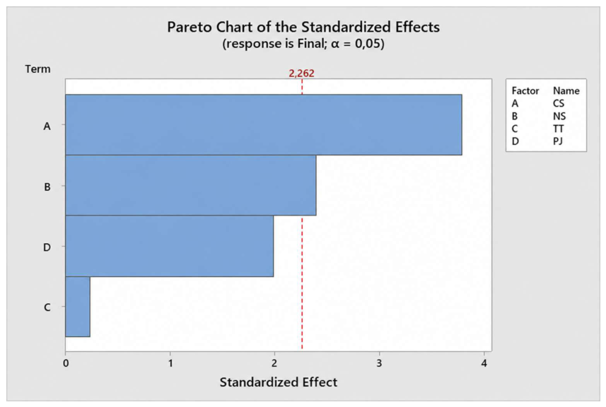
Figure 2.
Contour plot of LVI as a function of CS and NS.
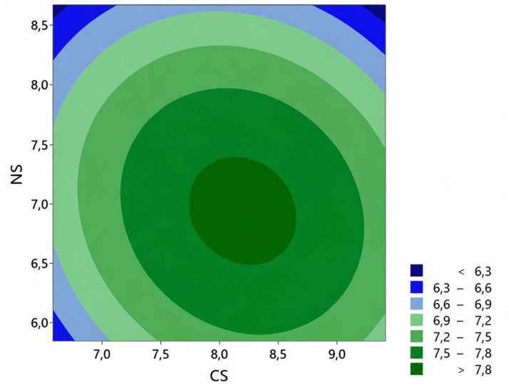
Figure 3.
Numerical optimization of LVI as a function of CS and NS.
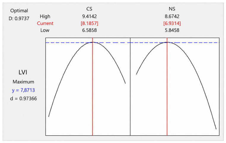
Figure 4.
PCA biplot of the variables measured during fermentation.
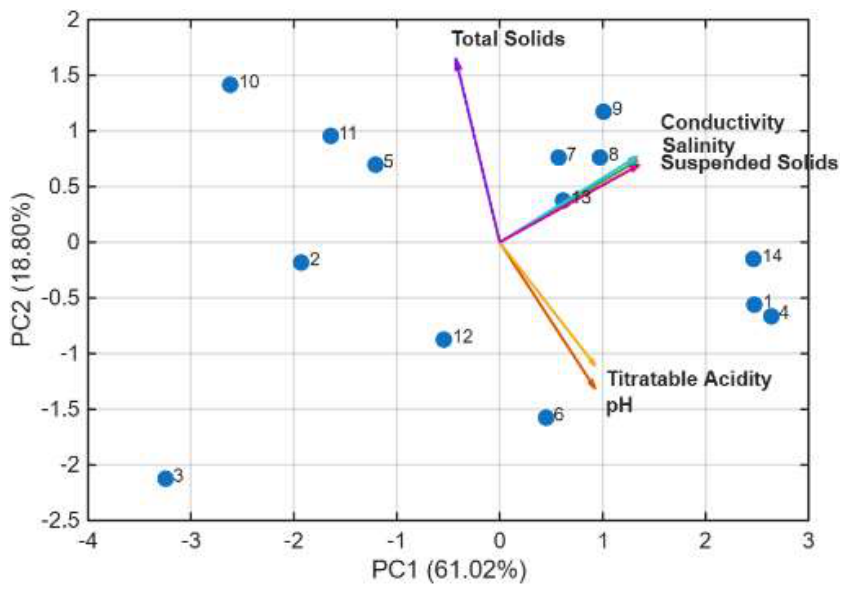
Figure 5.
PCA distribution according to LVI.
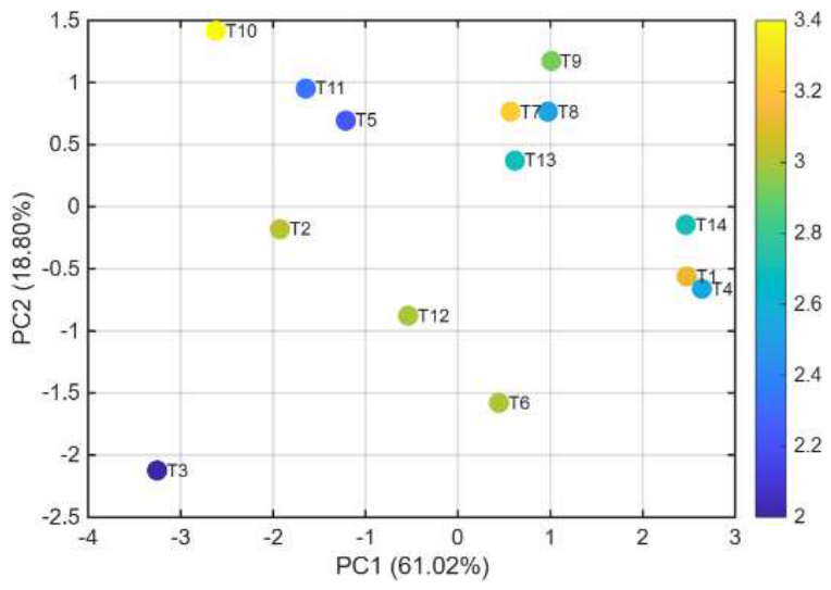
Table 1.
Independent variables and levels used in the screening design.
| Independent variables | Minimum level (-1) | Maximum level (+1) |
| Pumpkin juice in the activation medium, PJ (%) | 5% | 15% |
| Carbon source, CS (%) | 4% | 8% |
| Nitrogen source, NS (%) | 4% | 8% |
| Thermal treatment, TT | Sin | Con |
Table 3.
Experimental results obtained from the screening design.
| Run | CS (%) | NS (%) | TT | PJ (%) | LVI |
| 1 | 8 | 8 | Untreated | 15 | 3.12 |
| 2 | 4 | 4 | Treated | 15 | 3.02 |
| 3 | 6 | 6 | Treated | 10 | 2.00 |
| 4 | 4 | 8 | Treated | 10 | 2.55 |
| 5 | 6 | 4 | Untreated | 15 | 2.22 |
| 6 | 8 | 6 | Treated | 15 | 3.00 |
| 7 | 8 | 4 | Untreated | 10 | 3.23 |
| 8 | 4 | 6 | Untreated | 5 | 2.52 |
| 9 | 6 | 6 | Untreated | 10 | 2.92 |
| 10 | 8 | 4 | Treated | 5 | 3.40 |
| 11 | 4 | 4 | Treated | 5 | 2.33 |
| 12 | 6 | 8 | Treated | 5 | 3.00 |
| 13 | 8 | 8 | Untreated | 5 | 2.70 |
| 14 | 4 | 8 | Untreated | 15 | 2.70 |
Table 4.
Initial model for LVI.
| Model | Terms included |
(p)-value of the model | Terms | R2 (%) | R2 adjusted (%) | R2 predicted (%) | |||
| (p)-value | |||||||||
| CS | NS | TT | PJ | ||||||
| Initial | CS, NS, TT, PJ | 0.011 | 0.004 | 0.040 | 0.814 | 0.077 | 73.18 | 61.27 | 29.07 |
Table 6.
Path of maximum ascent calculated from the refined model.
| Step | CS (%) | NS (%) | PJ (%) | LIV |
| 0 | 6 | 6 | 10 | 5,85 |
| 1 | 7 | 6,63 | 8,64 | 7,38 |
| 2 | 8 | 7,26 | 7,28 | 8,17 |
| 3 | 9 | 7,88 | 5,92 | 6,19 |
| 4 | 10 | 8,51 | 4,56 | 6,20 |
Table 7.
Response surface design and experimental LVI values.
| Run | CS (%) | NS (%) | LIV |
| 1 | 7,00 | 6,26 | 7,149 |
| 2 | 9,00 | 6,26 | 7,499 |
| 3 | 7,00 | 8,26 | 6,999 |
| 4 | 9,00 | 8,26 | 7,149 |
| 5 | 6,59 | 7,26 | 6,922 |
| 6 | 9,41 | 7,26 | 7,301 |
| 7 | 8,00 | 5,85 | 7,661 |
| 8 | 8,00 | 8,67 | 6,264 |
| 9 | 8,00 | 7,26 | 7,903 |
| 10 | 8,00 | 7,26 | 7,145 |
| 11 | 8,00 | 7,26 | 7,071 |
| 12 | 8,00 | 7,26 | 7,149 |
| 13 | 8,00 | 7,26 | 7,752 |
Table 8.
Analysis of variance for the response surface design.
| Term | p-value |
| Model | <0.001 |
| CS | 0.022 |
| NS | 0.001 |
| CS × CS | <0.001 |
| NS × NS | <0.001 |
| CS × NS | 0.135 |
Table 9.
Observed and predicted LVI values for the response surface design.
| Run | CS (%) | NS (%) | Observed LVI | Predicted LVI |
| 1 | 7,00 | 6,26 | 7.299 | 7.135 |
| 2 | 9,00 | 6,26 | 7.698 | 7.539 |
| 3 | 7,00 | 8,26 | 6.998 | 6.914 |
| 4 | 9,00 | 8,26 | 6.996 | 6.936 |
| 5 | 6,59 | 7,26 | 6.844 | 6.982 |
| 6 | 9,41 | 7,26 | 7.300 | 7.284 |
| 7 | 8,00 | 5,85 | 7.476 | 7.420 |
| 8 | 8,00 | 8,67 | 6.694 | 6.838 |
| 9 | 8,00 | 7,26 | 7.903 | 7.827 |
| 10 | 8,00 | 7,26 | 7.903 | 7.827 |
| 11 | 8,00 | 7,26 | 7.903 | 7.827 |
| 12 | 8,00 | 7,26 | 7.902 | 7.827 |
| 13 | 8,00 | 7,26 | 7.902 | 7.827 |
| () (%) | 89,22 | |||
| () (%) | 84,31 | |||
| () (%) | 73,71 | |||
Table 10.
Triplicate validation of the optimized inoculum.
| Mean experimental LVI |
Predicted LVI | Relative error (%) | Standard error | 95% confidence interval | 95% prediction interval |
| 7.828 | 7.871 | 0.548 | 0.092 | 7.641–8.014 | 7.334–8.322 |
Disclaimer/Publisher’s Note: The statements, opinions and data contained in all publications are solely those of the individual author(s) and contributor(s) and not of MDPI and/or the editor(s). MDPI and/or the editor(s) disclaim responsibility for any injury to people or property resulting from any ideas, methods, instructions or products referred to in the content. |
© 2026 by the authors. Licensee MDPI, Basel, Switzerland. This article is an open access article distributed under the terms and conditions of the Creative Commons Attribution (CC BY) license (http://creativecommons.org/licenses/by/4.0/).
Copyright: This open access article is published under a Creative Commons CC BY 4.0 license, which permit the free download, distribution, and reuse, provided that the author and preprint are cited in any reuse.